On the Pricing of Longevity-Linked Securities!

Daniel Bauera, Matthias Borger!,b, Jochen Rußc

aDepartment of Risk Management and Insurance, Georgia State University, 35 Broad Street (11th Floor), Atlanta,GA 30303, USA

bInstitute of Insurance, Ulm University & Institute for Finance and Actuarial Science (ifa), Helmholtzstraße 22,89081 Ulm, Germany

cInstitute for Finance and Actuarial Science (ifa), Helmholtzstraße 22, 89081 Ulm, Germany

AbstractFor annuity providers, longevity risk, i.e. the risk that future mortality trends differ from those an-ticipated, constitutes an important risk factor. In order to manage this risk, new financial products,so-called longevity derivatives, may be needed, even though a first attempt to issue a longevitybond in 2004 was not successful.

While different methods of how to price such securities have been proposed in recent literature,no consensus has been reached. This paper reviews, compares and comments on these differentapproaches. In particular, we use data from the United Kingdom to derive prices for the proposedfirst longevity bond and an alternative security design based on the different methods.

Key words:longevity risk, stochastic mortality, longevity derivativesJEL classification: G13, G22Subj. class: IM53, IE50, IB10

1. Introduction

Longevity risk, i.e. the risk that the realized future mortality trend exceeds current assump-tions, constitutes an important risk factor for annuity providers and pension funds. This risk isincreased by the current problems of state-run pay-as-you-go pension schemes in many countries:The reduction of future benefits from public pension systems and tax incentives for annuitizationof private wealth implemented by many governments may lead to an increasing demand for an-nuities (cf. Kling et al. (2008)). One prevalent way of managing this risk is securitization, i.e.isolating the cash flows that are linked to longevity risk and repackaging them into cash flows that

!An earlier version of this paper entitled “Pricing Longevity Bonds Using Implied Survival Probabilities” waspresented at the 2006 meeting of the American Risk and Insurance Association (ARIA) and the 2006 meeting of theAsia-Pacific Risk and Insurance Association (APRIA). Moreover, some of the ideas have previously been presented inBauer (2008). We are grateful for valuable comments from participants of the 35th Seminar of the European Groupof Risk & Insurance Economists (EGRIE) and the 4th International Longevity Risk and Capital Markets SolutionsConference, in particular by Hato Schmeiser and Andrew Cairns, respectively.

!Corresponding author. Phone: +49 (731) 50 31230. Fax: +49 (731) 50 31239.Email addresses: dbauer@gsu.edu (Daniel Bauer), m.boerger@ifa-ulm.de (Matthias Borger),

j.russ@ifa-ulm.de (Jochen Ruß)

Preprint submitted to Elsevier November 30, 2008

ManuscriptClick here to view linked References

are traded in capital markets (see Cowley and Cummins (2005) for an overview of securitizationin life insurance).

In academic literature, several supporting instruments such as so-called longevity or survivorbonds (cf. Blake and Burrows (2001)) or survivor swaps (cf. Dowd et al. (2006)) have been pro-posed (see Blake et al. (2006a) for an overview). However, a first attempt to issue a longevity-linked security in 2004 failed (see Section 4 for more information). Nevertheless, the generalconsensus amongst practitioners appears to be that whilst a breakthrough is yet to come, “bettingon the time of death is set”,1 and several investment banks such as JPMorgan or Goldman Sachshave installed trading desks for longevity risk.

Aside from the question of how to appropriately engineer such longevity-linked securities orlongevity derivatives, there is an ongoing debate of how to price a given instrument. This debate istwofold: On one hand, there is a quest for actuarial or economic methods of how to derive prices“conceptually” and, on the other hand, there is the problem of how to derive prices given a certainmethodology – i.e. what data to use for calibration purposes.

In this paper, we address all of these issues. First, we review and compare different pricingmethods proposed in recent literature. Subsequently, we empirically compare different approachesbased on the established methods using data from the United Kingdom (UK). Moreover, we discussthe financial engineering aspect of longevity securitization and, based on this discussion, introduceand analyze a longevity derivative with option-type payoff. Thus, in addition to a long-neededtheoretical and empirical survey on proposed pricing approaches for longevity-linked securities,this paper provides several new ideas which could be helpful in building a market in longevity risk.

The pricing of longevity derivatives is of course closely related to modeling the stochastic evo-lution of mortality. So far, several stochastic mortality models have been proposed – for a detailedoverview and a categorization see Cairns et al. (2006b). We rely on a continuous-time stochasticmodeling framework for mortality. Milevsky and Promislow (2001) were among the first to pro-pose a stochastic hazard rate or force of mortality, Dahl (2004) presents a general stochastic modelfor the mortality intensity, and in Biffis (2005), affine jump-diffusion processes are employed tomodel both, financial and demographic risk factors. However, while in these articles the spot forceof mortality is modeled, we adopt the forward modeling approach for mortality (see Cairns et al.(2006b), Miltersen and Persson (2005), or Bauer et al. (2008)).

The remainder of the paper is organized as follows. In Section 2, we review pricing approachespresented in recent literature, and formalize as well as compare them in a common setting in Sec-tion 3. In particular, we point out technical problems with some of these approaches. Subsequently,we present an empirical comparison based on the first announced – but never issued – longevitybond, the so-called EIB/BNP-Bond, in Section 4. Aside from providing valuable insights on theadequacy of the different methods, our results reveal why different authors have come to differentappraisals of “how good of a deal” the EIB/BNP-Bond was. However, beyond the pricing, the fi-nancial engineering of the Bond may also have been a reason for its failure. We discuss this matterand, in Section 5, introduce and analyze an alternative security design with an option-type payoffstructure. Finally, Section 6 concludes.

1The Business, 08/15/2007, “Betting on the time of death is set”, by P. Thornton.

2

2. Different Approaches for Pricing Longevity-Linked Securities

The price a party is willing to pay for some longevity derivative depends on both, the estimateof uncertain future mortality trends and the level of uncertainty.2 This uncertainty is likely toinduce a mortality risk premium that should be priced by the market (cf. Milevsky et al. (2005)).However, so far, if at all, there are no liquidly traded securities. Therefore, it is not possible to relyon market data for pricing purposes.3 As a consequence, different methods for pricing mortalityrisk have been proposed.

Friedberg and Webb (2007) apply the Capital Asset Pricing Model (CAPM) and the Consump-tion Capital Asset Pricing Model (CCAPM) to quantify risk premiums for potential investors inlongevity bonds, which turn out to be very low. However, the authors acknowledge that there islikely to exist a “mortality premium puzzle” similar to the well-known “equity premium puzzle”(cf. Mehra and Prescott (1985)) implying higher mortality risk premiums than these economicmodels would suggest. Thus, their quantitative results seem to be of limited applicability and wewill not further discuss this approach.

Milevsky et al. (2005) and Bayraktar et al. (2008) develop a theory for pricing non-diversifiablemortality risk in an incomplete market: They postulate that an issuer of a life contingency re-quires compensation for this risk according to a pre-specified instantaneous Sharpe ratio (see alsoBayraktar and Young (2008)). They show that their pricing approach has several appealing prop-erties, which are particularly intuitive in a discrete-time setting (cf. Milevsky et al. (2006)). Thebasic idea is that an additional return in excess of the risk-free rate is paid on the insurer’s assetportfolio, which is determined as a multiple ! – the instantaneous Sharpe ratio – of the remainingstandard deviation after all diversifiable risk is hedged away. While for a finite number of insuredsthis approach leads to a non-linear partial differential equation for the price of an insurance con-tract, the pricing rule becomes linear as the portfolio size approaches infinity (see Milevsky et al.(2005)) – as it is clearly the case for an index-linked longevity derivative. Then, it can be shownthat their approach coincides with a change of the probability measure from the physical measureP to a “risk-adjusted” measure Q! invoked by a constant “market price of risk” process (cf. Bauer(2008), Subs. 3.2.1).

Similarly, other structures of the market price of mortality risk could be considered, too; basi-cally, we may choose any adapted, predictable process. However, as pointed out by Blake et al.(2006b), “one can argue that more sophisticated assumptions about the dynamics of the marketprice of longevity risk are pointless given that, at the time, there was [is] just a single item of pricedata available for a single date (and even that is no longer valid).” Even if a constant market priceof risk is chosen, the question of how to calibrate it remains open, although Milevsky et al. (2006)state that the “Sharpe ratio from stocks as an asset class” is approximately equal to !S&P = 0.25(Loeys et al. (2007) also report a level of 25%).

In order to account for a risk premium, Lin and Cox (2005, 2008) apply the so-called 1-factorand 2-factor Wang transform, respectively, to distort the best estimate cumulative distribution func-

2In order to keep our presentation concise, we turn our attention to pricing approaches for index-linked longevityderivatives. In particular, we do not consider indemnity securitization transactions, where small sample risk may needto be taken into account.

3Cairns et al. (2006b) calibrate their 2-factor model to published pricing data of the EIB/BNP-Bond. However, webelieve that relying on the published data is problematic since pricing may have been an issue for its failure.

3

tion of the future lifetime of an individual aged x. In order to find a suitable transform for pricingparticular longevity securities, i.e. to calibrate the transform parameters, the authors rely on marketprices of annuity contracts.

However, as pointed out by Pelsser (2008), the Wang transform does not provide “a universalframework for pricing financial and insurance risks” (cf. Wang (2002)), so the adequacy is ques-tionable.4 Moreover, it is not clear whether annuity prices offer an adequate starting point whenpricing longevity derivatives, and it is unclear “how different transforms for different cohorts andterms to maturity relate to one another and form a coherent whole” (cf. Cairns et al. (2006b)).

3. Methodological Comparison of the Pricing Approaches

In the previous section, we introduced pricing approaches for longevity-linked securities. In thecurrent section, we establish them in a common framework: We adopt the setup from Bauer et al.(2008), which is summarized in the first subsection. The second subsection then presents pricingformulae for simple longevity bonds under the different approaches. Finally, the last subsectionpoints out potential shortcomings of the transform-based approach from Lin and Cox (2005, 2008).

3.1. The Forward Mortality FrameworkFor the remainder of this paper, we fix a time horizon T ! and a filtered probability space

(!,F ,F, P ), where F = (Ft)0"t"T ! is assumed to satisfy the usual conditions. Furthermore, wefix a (large) underlying population of individuals, where each age cohort is denoted by the age x0

at time zero. We assume that the best estimate forward force of mortality with maturity T as fromtime t,

µt(T, x0) := !"

"Tlog

!

EP

"

T p(T )x0

#

#Ft

$% T>t= !

"

"Tlog

&

EP

'

T#tp(T )x0+t

#

#

#Ft

()

, (1)

is well defined, where T#tp(T )x0+t denotes the proportion of (x0 + t)-year olds at time t " T who

are still alive at time T , i.e. the survival rate or the “realized survival probability”. Moreover, weassume that (µt(T, x0))0"t"T satisfy the system of stochastic differential equations

dµt(T, x0) = #(t, T, x0) dt + $(t, T, x0) dWt, µ0(T, x0) > 0, x0, T # 0, (2)

where W = (Wt)t$0 is a d-dimensional standard Brownian motion independent of the financialmarket, and t $% #(t, T, x0) as well as t $% $(t, T, x0) are continuous functions. Hence, weare in the “Gaussian case”, i.e. the forward force of mortality could become negative for extremescenarios, but we regard this as an acceptable shortcoming for practical considerations. The driftcondition (cf. Bauer et al. (2008)) yields

#(t, T, x0) = $(t, T, x0) &

* T

t

$(t, s, x0)% ds,

4Several other authors also relied on the Wang transform for pricing longevity derivatives. See e.g. Denuit et al.(2007) or Loisel and Serant (2007).

4

and, by the definition (1), for the (T !t)-year best estimate survival probability for an (x0 +t)-yearold at time t, we have

EP

'

T#tp(T )x0+t

#

#

#Ft

(

= EP

'

e#R

T

tµs(s,x0) ds

#

#

#Ft

(

= e#R

T

tµt(s,x0) ds.

The price of any security is now given as the expected value of its payoff under some equivalentmartingale measure (see Harrison and Kreps (1979) or Duffie and Skiadas (1994)), which in turnis defined by its Radon-Nikodym density, say

"Q

"P

#

#

#

#

Ft

= exp

+* t

0

!(s)% dWs !1

2

* t

0

'!(s)'2 ds

,

,

where – for simplicity – we restrict ourselves to deterministic choices of the “market price of risk”process (!(t))t$0. Hence, we have

EQ

'

T#tp(T )x0+t

#

#

#Ft

(

= EQ

'

e#R

T

tµs(s,x0) ds

#

#

#Ft

(

= EQ

'

e#R

T

tµt(s,x0)+

R

s

t"(u,s,x0) du+

R

s

t#(u,s,x0) dWu ds

#

#

#Ft

(

= e#R

T

t

R

s

t#(u,s,x0) !(u) du ds & EQ

'

e#R

T

tµt(s,x0)+

R

s

t"(u,s,x0) du+

R

s

t#(u,s,x0) (dWu#!(u) du) ds

#

#

#Ft

(

= e#R

T

t

R

s

t#(u,s,x0) !(u) du ds & EP

'

T#tp(T )x0+t

#

#

#Ft

(

, (3)

since W =-

Wt

.

t$0with Wt = Wt !

/ t

0 !(u) du is aQ-Brownian motion by Girsanov’s Theorem(see e.g. Theorem 3.5.1 in Karatzas and Shreve (1991)). Therefore, for the “risk-neutral” forwardforce of mortality with maturity T as from time t,

µt(T, x0) := !"

"Tlog

&

EQ

'

T#tp(T )x0+t

#

#

#Ft

()

= µt(T, x0) +

* T

t

$(s, T, x0) !(s) ds, (4)

we also havedµt(T, x0) = #(t, T, x0) dt + $(t, T, x0) dWt (5)

by Ito’s Formula. In particular, for the time zero “price” of a basic (T, x0)-Longevity Bond, whichpays T p

(T )x0at time T (cf. Cairns et al. (2006b)), we have

"0 (T, x0) := p(0, T ) EQ

"

T p(T )x0

$

= e#R

T

0µ0(s,x0)+f(0,s) ds,

where p(0, T ) is the time zero price of a zero-coupon bond with maturity T and f(0, s) is theforward force of interest (see e.g. Bjork (1999)).

From a practical point of view, this definition could be problematic: In reality, at time T , T p(T )x0

can only be approximated from a finite amount of data and this approximation may not be avail-able until months or even years after time T (cf. Cairns et al. (2006b)). However, similarly to theEIB/BNP-Bond, payments could be postponed by a deferral period. Moreover, several investmentbanks are working on establishing real-time longevity indices such as Goldman Sachs’ QxX index(see http://www.qxx-index.com/) or JPMorgan’s LifeMetrics Index (see http://www.lifemetrics.com).

5

It is important to note that we do not assume that (T, x0)-Longevity Bonds are liquidly availablein the market. In fact, when assuming that a sufficient number of (T, x0)-Longevity Bonds weretraded, by the same argumentation as in Heath et al. (1992) for financial bonds, under weak condi-tions on the volatility structure, the market would be complete. In particular, the measureQ wouldbe uniquely determined, such that basically all longevity derivatives would have a well-determinedprice – and that is clearly unrealistic. Hence, the quantities "0 (T, x0) should be interpreted astechnical auxiliary definitions, which rather simplify the presentation than denote prices of securi-ties that are actually traded; this is similar to interest rate modeling, where zero-coupon bonds areemployed as the basic building blocks.

Their particular usefulness under our specification becomes evident when regarding Equation(3): When given best estimate dynamics (2), which can be inferred from historic data, it is sufficientto know the “market price of risk” process (function) (!(t))t$0 in order to specify the “risk-neutral”(pricing) model (cf. Eq. (4) and (5)). By Equation (3), we immediately get

"0 (T, x0) = p(0, T ) T px0= e#

R

T

0

R

s

0#(u,s,x0) !(u) du ds p(0, T ) T px0

, (6)

where T px0= EP

'

T p(T )x0

(

and T px0= EQ

'

T p(T )x0

(

. Thus, specifying the “market price of risk” isequivalent to specifying "0 (T, x0), i.e. pricing (T, x0)-Longevity Bonds.

3.2. Pricing Simple Longevity BondsFor pricing a (T, x0)-Longevity Bond, the idea of Lin and Cox (2005) corresponds to applying

the 1-factor Wang transform to the best estimate mortality probability, i.e.

1 ! T px0= #

0

##1 (1 ! T px0) ! %

1

,

where #(·) is the cumulative distribution function of the standard Normal distribution and % is theparameter of the Wang transform. Hence, under this approach we have (cf. Eq. (6))

"0 (T, x0) = p(0, T )0

1 ! #0

##1 (1 ! T px0) ! %

11

. (7)

A similar equation can be found for the 2-factor Wang transform applied in Lin and Cox (2008).As pointed out in Section 2, pricing (T, x0)-Longevity Bonds using a “pre-specified instanta-

neous Sharpe ratio” ! in the 1-factor model from Milevsky et al. (2005) corresponds to a constantmarket price of risk. However, in our model setup, we allow for a multi-dimensional Brownianmotion – and thus a multi-dimensional market price of risk process. By an application of Ito’sproduct formula, we obtain

limh&0

2

1

hVarP [ µt+h(T, x0)| Ft] =

3

4

4

5

d6

i=1

($i(t, T, x0))2,

where clearly $i is the ith component of the volatility function $. Thus, in the multi-dimensional

6

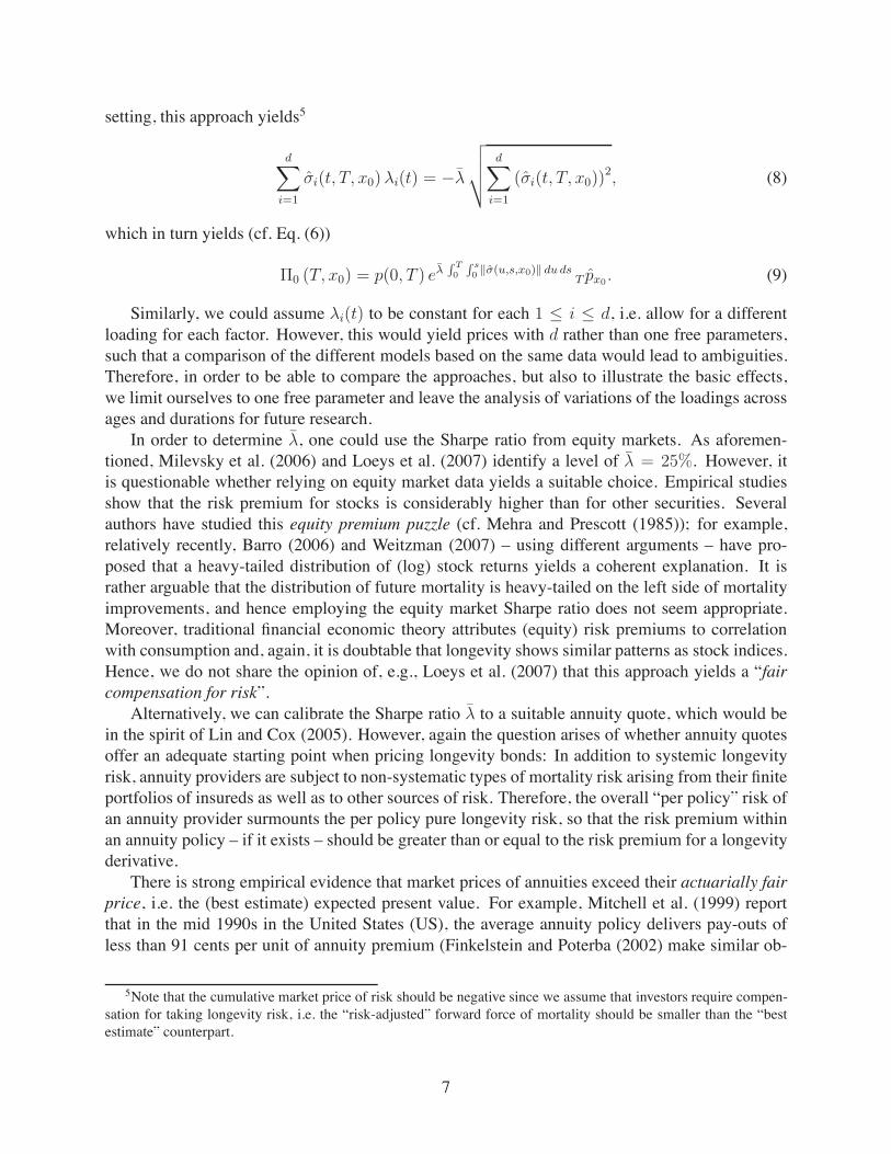
setting, this approach yields5

d6

i=1

$i(t, T, x0) !i(t) = !!

3

4

4

5

d6

i=1

($i(t, T, x0))2, (8)

which in turn yields (cf. Eq. (6))

"0 (T, x0) = p(0, T ) e!R

T

0

R

s

0'#(u,s,x0)' du ds

T px0. (9)

Similarly, we could assume !i(t) to be constant for each 1 " i " d, i.e. allow for a differentloading for each factor. However, this would yield prices with d rather than one free parameters,such that a comparison of the different models based on the same data would lead to ambiguities.Therefore, in order to be able to compare the approaches, but also to illustrate the basic effects,we limit ourselves to one free parameter and leave the analysis of variations of the loadings acrossages and durations for future research.

In order to determine !, one could use the Sharpe ratio from equity markets. As aforemen-tioned, Milevsky et al. (2006) and Loeys et al. (2007) identify a level of ! = 25%. However, itis questionable whether relying on equity market data yields a suitable choice. Empirical studiesshow that the risk premium for stocks is considerably higher than for other securities. Severalauthors have studied this equity premium puzzle (cf. Mehra and Prescott (1985)); for example,relatively recently, Barro (2006) and Weitzman (2007) – using different arguments – have pro-posed that a heavy-tailed distribution of (log) stock returns yields a coherent explanation. It israther arguable that the distribution of future mortality is heavy-tailed on the left side of mortalityimprovements, and hence employing the equity market Sharpe ratio does not seem appropriate.Moreover, traditional financial economic theory attributes (equity) risk premiums to correlationwith consumption and, again, it is doubtable that longevity shows similar patterns as stock indices.Hence, we do not share the opinion of, e.g., Loeys et al. (2007) that this approach yields a “faircompensation for risk”.

Alternatively, we can calibrate the Sharpe ratio ! to a suitable annuity quote, which would bein the spirit of Lin and Cox (2005). However, again the question arises of whether annuity quotesoffer an adequate starting point when pricing longevity bonds: In addition to systemic longevityrisk, annuity providers are subject to non-systematic types of mortality risk arising from their finiteportfolios of insureds as well as to other sources of risk. Therefore, the overall “per policy” risk ofan annuity provider surmounts the per policy pure longevity risk, so that the risk premium withinan annuity policy – if it exists – should be greater than or equal to the risk premium for a longevityderivative.

There is strong empirical evidence that market prices of annuities exceed their actuarially fairprice, i.e. the (best estimate) expected present value. For example, Mitchell et al. (1999) reportthat in the mid 1990s in the United States (US), the average annuity policy delivers pay-outs ofless than 91 cents per unit of annuity premium (Finkelstein and Poterba (2002) make similar ob-

5Note that the cumulative market price of risk should be negative since we assume that investors require compen-sation for taking longevity risk, i.e. the “risk-adjusted” forward force of mortality should be smaller than the “bestestimate” counterpart.

7

servations for the UK). From the policyholder’s point of view, the price of the annuity contract maybe interpreted as the fair price plus some individual utility premium. From the insurer’s perspec-tive, on the other hand, the amount exceeding the fair price may consist of several components.While according to Mitchell et al. (1999) this “transaction cost” is primarily due to expenses, profitmargins, and contingency funds, Milevsky and Young (2007) do not believe that these fees can beclassified “under the umbrella of transaction costs”. They rather think the fees are “inseparablylinked to aggregate mortality risk”. Weale and Van de Ven (2006) come to a similar conclusion:Annuitization costs due to aggregate longevity uncertainty arise endogenously in their two periodoverlapping generation general equilibrium model.

Therefore, we conclude that it is very plausible for life annuities to include a risk premium forlongevity risk, and there is evidence that this risk premium accounts for a significant part of theamount exceeding the actuarially fair price. In particular, estimates of the longevity risk premiumbased on annuity prices will at least provide an upper bound for the risk premium to be included inlongevity derivative pricing. The question of how close this bound will be depends on the relativeinfluence of other factors on annuity prices, and particularly on the question of whether or notannuities include risk premiums for other sources of risk such as non-systematic mortality risk.

While there does not seem to be a distinct answer, at least for non-systematic mortality risk, wesee evidence that this is not the case: On one hand, Brown and Orszag (2006) note that “insurers areextremely adept at using the LLN (Law of Large Numbers) to essentially eliminate the relevanceof idiosyncratic risk facing any one individual that they insure.” On the other hand, if there werea charge for non-systematic mortality risk, this charge would clearly depend on the number ofinsureds within an insurer’s portfolio, so that large insurers would have a significant advantage.This, in turn, would eventually lead to a market with only few, large insurers, which clearly is notthe case in many developed markets.

Hence, although the validity of the idea by Lin and Cox (2005) to rely on annuity marketdata for deriving longevity derivative prices cannot be conclusively confirmed, we believe thatthis approach offers valuable insights at the current stage of the market with little or no longevityderivatives traded and considering the proposed alternatives such as relying on premiums for utterlydifferent types of risks. In particular, the results will at least provide upper bounds for the prices ofsimple longevity bonds, so together with the actuarially fair price we obtain a price interval for anylongevity derivative. However, we still need to address the question of whether their application ofthe Wang transform is adequate and leads to “coherent” prices (cf. Sec. 2).

3.3. Shortcomings of the Approach by Lin and Cox (2005, 2008)As explained above, the pricing approaches of Lin and Cox (2005, 2008) can be interpreted

as transforms of best estimate survival probabilities T px0, T, x0 # 0 (or equivalently, the forward

force of mortality surface at time zero (µ0(T, x0))T,x0$0), to match observed insurance prices.However, it is not clear if the application of an arbitrary transform is suitable; in particular, thesuitability of the Wang transform is of interest.

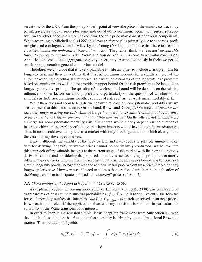
In order to keep this discussion simple, let us adapt the framework from Subsection 3.1 withthe additional assumption that d = 1, i.e. that mortality is driven by a one-dimensional Brownianmotion. Then, Equation (4) yields

µ0(T, x0) ! µ0(T, x0) = !

* T

0

$(s, T, x0) !(s) ds. (10)

8

On the other hand, if “risk-neutral” forward forces are derived from best estimate forward forcesvia some transform, say O(·), we have

O (µ0(·, ·)) (T, x0) = µ0(T, x0),

i.e. we are given the left-hand side of (10), and in order to derive the implied market price of riskwe may solve for (!(t))t$0.

For each fixed x0, (10) is a Volterra integral equation of the first kind, and under weak regularityconditions, there exists a unique solution, say (!x0

(t))t$0 (see e.g. Subs. 7.2.1.2 in Polyanin andManzhirov (1999)). Now consider another age group (cohort), say x1. If there exists some T suchthat

O (µ0(·, ·)) (T, x1) (= µ0(T, x1) +

* T

0

$(s, T, x1) !x0(s) ds,

then (10) does not have a solution, i.e. the market price of risk process for different ages – but forthe same source of risk – will be different, which clearly leads to arbitrage opportunities as soon aslongevity derivatives on both cohorts are traded. Hence, under the current assumptions, the onlysuitable transforms are of the form

O!(·) (µ0(·, ·)) (T, x0) := µ0(T, x0) +

* T

0

$(s, T, x0) !(s) ds

for some given !(·) or, equivalently, of the form (3) for the best estimate survival survival proba-bilities. In particular, the Wang transform does not present a suitable choice in this framework assoon as there are at least two different longevity derivatives traded based on at least two cohortseven when allowing for different transform parameters for different cohorts.

While this inconsistency is only shown under the current assumptions, our results indicatedrawbacks associated with the methodology from Lin and Cox (2005, 2008). Nevertheless, forpractical applications and when only pricing a longevity derivative based on a single cohort, theWang transform still presents a theoretically valid approach – the question of whether it is adequate,however, prevails.

4. Empirical Comparison Based on the EIB/BNP Longevity Bond

In this section, we compare the pricing approaches introduced in Section 2 from an empiri-cal perspective adopting the Gaussian forward mortality model proposed by Bauer et al. (2008).Alongside the Wang transform parameters derived by Lin and Cox (2005, 2008) and the instanta-neous Sharpe ratio from equity markets (cf. Subs. 3.2), we use a time series of UK annuity marketquotes to derive parameter estimates for different points in time.

4.1. “The Volatility of Mortality”Bauer et al. (2008) propose a volatility specification and, hence, a model for the best estimate

forward force of mortality µt(T, x0) in the framework introduced in Subsection 3.1. The modelequations are provided in Appendix A; for details on the volatility structure, resulting character-istics of the model, and the calibration algorithm, we refer to their paper. However, since theirestimates are based on US pensioner mortality data, for our objective it is necessary to recalibratethe model to UK data. We rely on UK life tables and projections for pension annuities as published

9

on the website of the Institute of Actuaries and the Faculty of Actuaries.6 Details on the employedtables as well as the resulting parameter estimates are also presented in Appendix A.

As explained in Section 3, only a market price of longevity risk (!(t))t$0 is still needed to havea fully specified pricing model at hand. This gap will be filled in the following subsection.

4.2. Pricing MethodsIn order to compare the pricing approaches by Lin and Cox (2005, 2008) and Milevsky et al.

(2005) based on the model introduced in the previous subsection, we derive Sharpe ratios andWang transform parameters from a monthly time series of UK pension annuity quotes from Jan-uary 2000 until December 2006.7 We consider quotes for single premium compulsory pensionannuities payable monthly in advance on 65-year old male lives without guarantee period. Foreach date, we take the average of all available quotes.8 In order to analyze the risk premium,administrative charges need to be eliminated. We assume up-front charges # between 1.5% and2% and an investment fee of 7 basis points of the technical reserve p.a. (see also Bauer and Weber(2008)). Moreover, we rely onWoolhouse’s summation formula (cf. Bowers et al. (1997)) to derivethe corresponding quotes R for annually paying annuities. The resulting present values are thenequated with their theoretical counterparts given a certain pricing approach. For example, underthe assumption of a constant instantaneous Sharpe ratio, we obtain

£10, 000 (1! #) = R

(6

k=0

1

(1 + ik ! 0.0007)k T px0

= R

(6

k=0

1

(1 + ik ! 0.0007)ke!

R

k

0

R

s

0'#(u,s,x0)' du ds

T px0, (11)

where ik is the annualized interest rate for k years, and the second equation follows from Equations(3) and (8).

For each annuity quote, the interest rates are taken from the UK government bonds yield curvefor the first working day of the corresponding month as published by the Bank of England.9 Sincethe yield curve is only given for maturities up to 25 years, we assume a flat yield curve thereafter.

The best estimate survival probabilities T px0for 2000 to 2006 are obtained from the following

mortality tables: For the first set of annuity quotes (01/2000 - 11/2002), we use the 92 Life OfficePensioners’ mortality table published by the Institute of Actuaries and the Faculty of Actuaries in1999; in December 2002, adjusted mortality projections were published for this mortality tableand, hence, from 12/2002 until 11/2005, we use the newly constructed medium cohort projectionwhich implies stronger mortality improvements than the original projection; for the remainingquotes (12/2005 - 12/2006), we rely on an even stronger projection based on the average of five

6http://www.actuaries.org.uk.7Data provided byMoneyfacts.co.uk Ltd.8The number of available quotes falls between 9 and 14 for each month.9Downloaded from http://www.bankofengland.co.uk/statistics/yieldcurve/index.htm on 01/13/2008. The interest

rates are to reflect the default risk faced by a policyholder, i.e. the risk that he does not receive his annuity payments atsome point. We use the UK government bonds yield curve here since such a scenario seems extremely unlikely as theFinancial Services Compensation Scheme will step in if an insurer is not able to meet its obligations.

10

-0.3-0.25-0.2-0.15-0.1-0.05

00.050.10.150.20.25

12/2000 12/2002 12/2004 12/2006

Sharpe ratios

Sharpe ratiosSharpe ratios (interpol.)

10-year interest rates (scaled)FTSE 100 (scaled)

-0.3

-0.2

-0.1

0

0.1

0.2

0.3

0.4

0.5

12/2000 12/2002 12/2004 12/2006

1-factor Wang transform parameters

Wang parametersWang parameters (interpol.)10-year interest rates (scaled)

FTSE 100 (scaled)-0.3

-0.2

-0.1

0

0.1

0.2

0.3

0.4

0.5

12/2000 12/2002 12/2004 12/2006

2-factor Wang transform parameters

Wang parametersWang parameters (interpol.)10-year interest rates (scaled)

FTSE 100 (scaled)

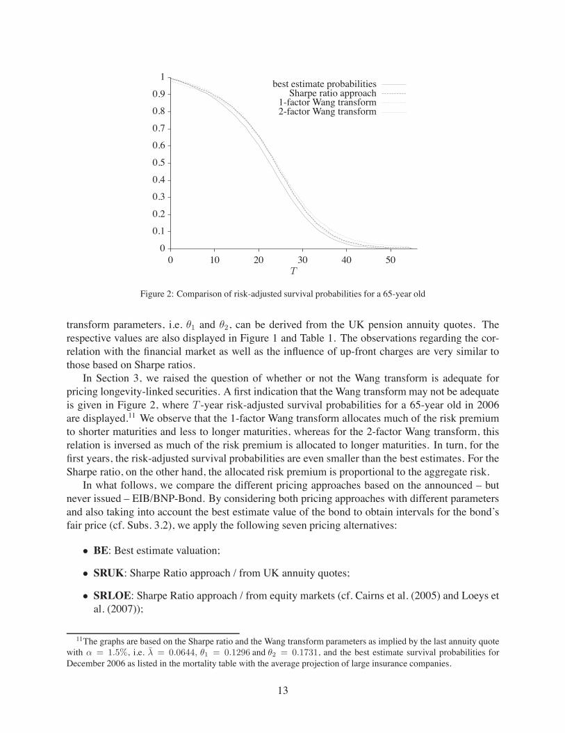
Figure 1: Evolution of the market price of longevity risk

projections used by different large insurance companies at that time as presented by Grimshaw(2007).

However, the underlying assumption of sudden changes in the best estimate survival probabili-ties when switching from one projection to the next is questionable in our setup: The derivation ofa new mortality projection clearly indicates that the existing projection does not yield best estimateprobabilities anymore. Therefore, in addition to the assumption of piecewise constant mortalityprojections, we also derive Sharpe ratios and Wang transform parameters under the assumptionof gradual changes in expected mortality, i.e. we interpolate linearly between the original 92 LifeOffice Pensioners’ mortality table for January 2000, the mortality table resulting from the mediumcohort projection in December 2002, and the mortality table based on the average projection oflarge insurance companies in December 2005. In both cases, solving Equation (11) for ! for eachannuity quote gives a time series of Sharpe ratios. For up-front charges of # = 1.5%, the timeseries are displayed in the top panel of Figure 1, together with the corresponding time series ofscaled 10-year interest rates and scaled FTSE 100 closing prices.10

Obviously, the approach of interpolated mortality tables leads to smaller Sharpe ratios due tolarger best estimate probabilities and does not exhibit jumps at the regime breaks. Moreover, weobserve that, in both cases, the Sharpe ratios implied by the first annuity quotes are negative, which

10FTSE 100 data downloaded from http://www.livecharts.co.uk/historicaldata.php on 03/03/2008.

11

# Sharpe ratios 1-factor Wang parameters 2-factor Wang parameters1.5% 0.0483 0.0787 0.1311

11/2002 1.75% 0.0427 0.0691 0.12102.0% 0.0371 0.0597 0.11101.5% 0.1209 0.2438 0.3008

11/2004 1.75% 0.1166 0.2333 0.28982.0% 0.1122 0.2228 0.27881.5% 0.0701 0.1424 0.1860

11/2006 1.75% 0.0660 0.1331 0.17642.0% 0.0618 0.1239 0.1667

Table 1: Market prices of longevity risk implied by UK pension annuities

means that, at that time, insurers assumed lower survival probabilities than listed in the respectivemortality table and/or higher expected investment returns than the risk-free interest rate: Until2000, insurers made large profits from equity investments which may have led them to promiserather high yields to policyholders. However, from September 2000 to March 2003, the FTSE 100crashed by approximately 46%, which then may have forced insurers to lower the offered yieldsresulting in an increase of the Sharpe ratios. The correlation between the Sharpe ratio and theFTSE 100 during this period is -0.800 in contrast to a correlation between Sharpe ratios and 10-year interest rates of only -0.182. In the subsequent time period until 2006, on the other hand, thecorrelation between Sharpe ratios and FTSE 100 drops to -0.496 and, hence, insurers seem to havesignificantly reduced – but not rendered – their exposure to equity returns.

If insurers never changed their annuity quotes, the correlation between the Sharpe ratio andthe 10-year interest rate would of course be very high. If insurers used pricing rates that moveparallel with interest rate shifts, on the other hand, this correlation would be very close to 0. Theobserved correlation for the time period from March 2003 to December 2006 is 0.907. To someextent, this might be simply due to a delayed reaction by insurers to changing interest rates asannuity rates usually are not adjusted on a daily basis. Another explanation might be drawn fromthe competition in the annuity market: In a scenario of falling interest rates, no insurer may wantto be the first to reduce the annuity rate as the company would loose out on new business. On theother hand, if interest rates increase, the insurer might want to keep a larger profit margin by notimmediately increasing its annuity rate. All these effects would result in annuity quotes somewhatsmoothing out interest rate movements.

As mentioned above, the Sharpe ratios displayed in Figure 1 have been derived under the as-sumption of an up-front charge parameter # = 1.5%. Assuming larger up-front charges obviouslyresults in smaller Sharpe ratios. However, the overall influence of the parameter # is rather small.In Table 1, the Sharpe ratios for November 2002, November 2004 and November 2006 are dis-played for different choices of #. We find that that increasing # from 1.5% to 2.0% reduces theSharpe ratio by only about 0.01, i.e. the influence of the up-front charge is not very pronounced.Moreover, we observe that, for all three dates, the Sharpe ratios implied by UK pension annuitiesare significantly smaller than the one of equity markets.

In an analogous fashion to the Sharpe ratio approach, values for the 1-factor and 2-factor Wang

12

0

0.1

0.2

0.3

0.4

0.5

0.6

0.7

0.8

0.9

1

0 10 20 30 40 50T

best estimate probabilitiesSharpe ratio approach

1-factor Wang transform2-factor Wang transform

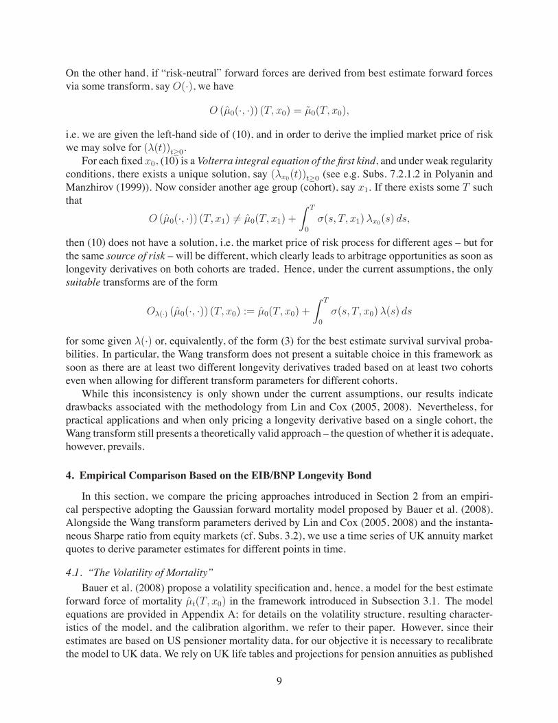
Figure 2: Comparison of risk-adjusted survival probabilities for a 65-year old

transform parameters, i.e. %1 and %2, can be derived from the UK pension annuity quotes. Therespective values are also displayed in Figure 1 and Table 1. The observations regarding the cor-relation with the financial market as well as the influence of up-front charges are very similar tothose based on Sharpe ratios.

In Section 3, we raised the question of whether or not the Wang transform is adequate forpricing longevity-linked securities. A first indication that the Wang transform may not be adequateis given in Figure 2, where T -year risk-adjusted survival probabilities for a 65-year old in 2006are displayed.11 We observe that the 1-factor Wang transform allocates much of the risk premiumto shorter maturities and less to longer maturities, whereas for the 2-factor Wang transform, thisrelation is inversed as much of the risk premium is allocated to longer maturities. In turn, for thefirst years, the risk-adjusted survival probabilities are even smaller than the best estimates. For theSharpe ratio, on the other hand, the allocated risk premium is proportional to the aggregate risk.

In what follows, we compare the different pricing approaches based on the announced – butnever issued – EIB/BNP-Bond. By considering both pricing approaches with different parametersand also taking into account the best estimate value of the bond to obtain intervals for the bond’sfair price (cf. Subs. 3.2), we apply the following seven pricing alternatives:

• BE: Best estimate valuation;

• SRUK: Sharpe Ratio approach / from UK annuity quotes;

• SRLOE: Sharpe Ratio approach / from equity markets (cf. Cairns et al. (2005) and Loeys etal. (2007));

11The graphs are based on the Sharpe ratio and the Wang transform parameters as implied by the last annuity quotewith ! = 1.5%, i.e. " = 0.0644, #1 = 0.1296 and #2 = 0.1731, and the best estimate survival probabilities forDecember 2006 as listed in the mortality table with the average projection of large insurance companies.

13

• 1WTUK: 1-Factor Wang transform / from UK annuity quotes;

• 1WTLC: 1-Factor Wang transform / from Lin and Cox (2005);

• 2WTUK: 2-Factor Wang transform / from UK annuity quotes;

• 2WTLC: 2-Factor Wang transform / from Lin and Cox (2008).

4.3. Comparison of Different Assessments of the EIB/BNP-BondIn November 2004, BNP announced the issuance of the first publicly traded longevity bond,

the so-called EIB/BNP-Bond. While it was withdrawn for redesign in 2005, it still has attractedconsiderable attention in academia as well as among practitioners.12

The notes were to be issued by the European Investment Bank (EIB), and the longevity riskwas to be taken by the Bahama-based reinsurer Partner Re. BNP was the originator and structurerof the deal. The basic design is quite simple: Investors in the bond were entitled to receive variablecoupon payments contingent on the mortality experience of English and Welsh males aged 65 in2003. The coupons C(t), t = 1, 2, ..., 25, were set to

C(t) = S(t) £50mn, where S(t) = S(t ! 1) (1 ! m(64 + t, 2002 + t)) and S(0) = 1.

Here, m(x, z) denotes the central death rate for an x-year old in year z as published by the Officefor National Statistics. Note that there is a time lag of two years between the end of the referenceperiod and the payment date since the mortality experience has to be assessed statistically.

Thus, holding such a security is similar to holding a portfolio of (k, 65)-longevity bonds asintroduced in Section 3 for k = 1, ..., 25 in 2003, but the payments are delayed by two years andthe definition here is based on central death rates rather than mortality probabilities. Now, if moreindividuals survive than anticipated, coupon payments will be higher; thus, for the next 25 years,the notes serve as an almost perfect hedge for an annuity provider whose portfolio of insuredscoincides with the reference population.

The total “value” of the issue was £540mn, and the offer price was determined by taking sur-vival rates as projected by theUKGovernment Actuary’s Department and discounting the projectedcoupon payments at LIBOR minus 35bps. Since, due to its S&P AAA rating, the EIB’s yield curveaveraged at approximately LIBOR-15, the remaining spread of about 20bps can be interpreted asthe fee investors had to pay for the hedge. Lin and Cox (2008) believe that the charged risk pre-mium is very high making the bond unattractive for potential investors. Contrarily, Cairns et al.(2005) figure that this price seems reasonable, even though “it is difficult to judge precisely howgood a deal the pension funds are [were] being offered”. It is worth noting that the authors basetheir conclusions on similar pricing methods to those introduced in Section 2: While Lin and Cox(2008) rely on comparisons of “risk premiums” implied by annuity prices and the EIB/BNP-Bondas parameters in corresponding Wang transforms, Cairns et al. (2005) take the EIB/BNP risk-premium relative to its “volatility” – i.e. the Sharpe ratio – and compare it to equity risk premiums.Thus, their method is in line with the ideas of Milevsky et al. (2005).

12The following short description of the security is based on Azzopardi (2005), Blake et al. (2006a), and Cairns etal. (2005). See their presentations for more details.

14

11/2002 11/2004 11/2006Actual na 540 naBE 512.80 528.85 548.15SRUK 520.25 550.33 561.68SRLOE 555.10 576.16 600.941WTUK 527.16 569.67 572.841WTLC 544.75 559.42 578.892WTUK 526.83 566.71 568.492WTLC 530.36 544.36 563.23

Table 2: Prices of EIB-type bonds using different pricing methods

In order to explain these different assessments of the EIB/BNP-Bond, we apply the sevenpricing methods defined in the previous subsection. In addition, we price two “artificial” bonds ofthe same structure but assuming that they would have been offered two years earlier and two yearslater, i.e. in November 2002 and November 2006, respectively, in order to analyze the influence ofdifferent Sharpe ratios and Wang transform parameters on the bond price. The exact issue datesare assumed to be the 18th of the respective months and the corresponding Sharpe ratios and Wangtransform parameters are shown in Table 1. The best estimate survival rates are taken from themortality projections of the UK Government Actuary’s Department from 2001, 2003 and 2004, i.e.the most recent mortality projection in each case, and the reference cohort is aged 65 in 2001, 2003and 2005, respectively. The interest rates are taken from the EIB’s yield curve at the respectivedates.13 The resulting bond prices are shown in Table 2.

We observe that the bond prices for the same pricing method differ considerably between theissue dates. This is due to different interest rates and changes in the mortality projections as well asto changes in the Sharpe ratio andWang transform parameters in case these have been derived fromthe UK annuity quotes. There are also significant differences between the pricing methods for thesame issue date resulting from the varying risk premium allocations and/or market prices of risk.However, the most striking observation is that, for all six “risk-adjusting” pricing methods, theprice of the EIB/BNP-Bond exceeds the £540mn requested by BNP. Hence, our analyses indicatethat the bond was indeed a rather “good deal”. Even when assuming that only a part of the mark-up within annuity quotes can be attributed to aggregate longevity risk, the fact that the suggestedprice lies approximately in the middle of best estimate and “risk-adjusted” values based on annuityprices suggests that the pricing was at least reasonably fair. From this observation, two questionsarise immediately:

• Why do Lin and Cox (2008) regard the bond as too expensive?

• And why was the bond not successfully placed?

The first question is quite simple to answer as Lin and Cox (2008) use different interest rates(gilt STRIPS) and, in particular, different best estimate survival rates, namely rates based on “real-ized mortality rates of English and Welsh males aged 65 and over in 2003”. Especially in the long

13Data downloaded from Bloomberg on 10/24/2008.

15

term, these survival rates are significantly smaller than those projected by the UK GovernmentActuary’s Department resulting in a lower “fair” price of the bond.

The second question is more difficult to answer. One reason might be the fact that the bondwas based on population mortality experience of a specific cohort rather than annuitants’ mortalityexperience implying basis risk (cf. Lin and Cox (2008)). However, as exhibited by Cairns et al.(2005), differences in mortality improvements between the general and the assured population arenot very pronounced, even though this observation may differ for a particular insurer’s portfolio.Other potential reasons have been pointed out, e.g. that the Bahama-based reinsurer Partner Re wasnot perceived to be a natural holder of UK longevity risk. However, probably the most striking ex-planations lie in the fixed maturity and the high upfront capital expense (see Cairns et al. (2005)):Due to the fixed maturity of 25 years, insurers and pension funds purchasing the bond would stillbe stuck with the tail risk, i.e. the longevity risk for high ages in the far future; moreover, the se-curitization of the “complete” survivor index takes capital away which may be used to hedge othersources of risk or to speculate in capital markets. After all, insurers are financial service providersmeaning that investing in capital markets can be regarded as one of their core competences.

To sum up, aside from basis risk, the financial engineering of the EIB/BNP-Bond may presentan important reason for its failure. Thus, in the next section, we propose a differently designedlongevity derivative, which overcomes some of the stylized deficiencies.

5. An Option-Type Longevity Derivative

As explained in the previous section, the EIB/BNP-Bond may not seem very attractive to in-surers. Therefore, we propose a differently designed derivative here: a call option-type longevityderivative with a payoff of the form14

CT =0

T p(T )x0

! K(T )1+

at time T , where K(T ), 0 " K(T ) " 1, is some threshold or strike, for example

K(T ) = (1 + a) EP

"

T p(T )x0

$

, a > 0.

This security or a combination of securities of this type overcome several deficiencies of theEIB/BNP-Bond and could thus be more appealing to insurers. For example, the insurer keepsthe “equity tranche” of the longevity risk exposure in its own books and only passes over the riskof extreme longevity. In particular, this will significantly decrease the committed capital. We referto Bauer (2008), Section 5.1, for a more detailed discussion.

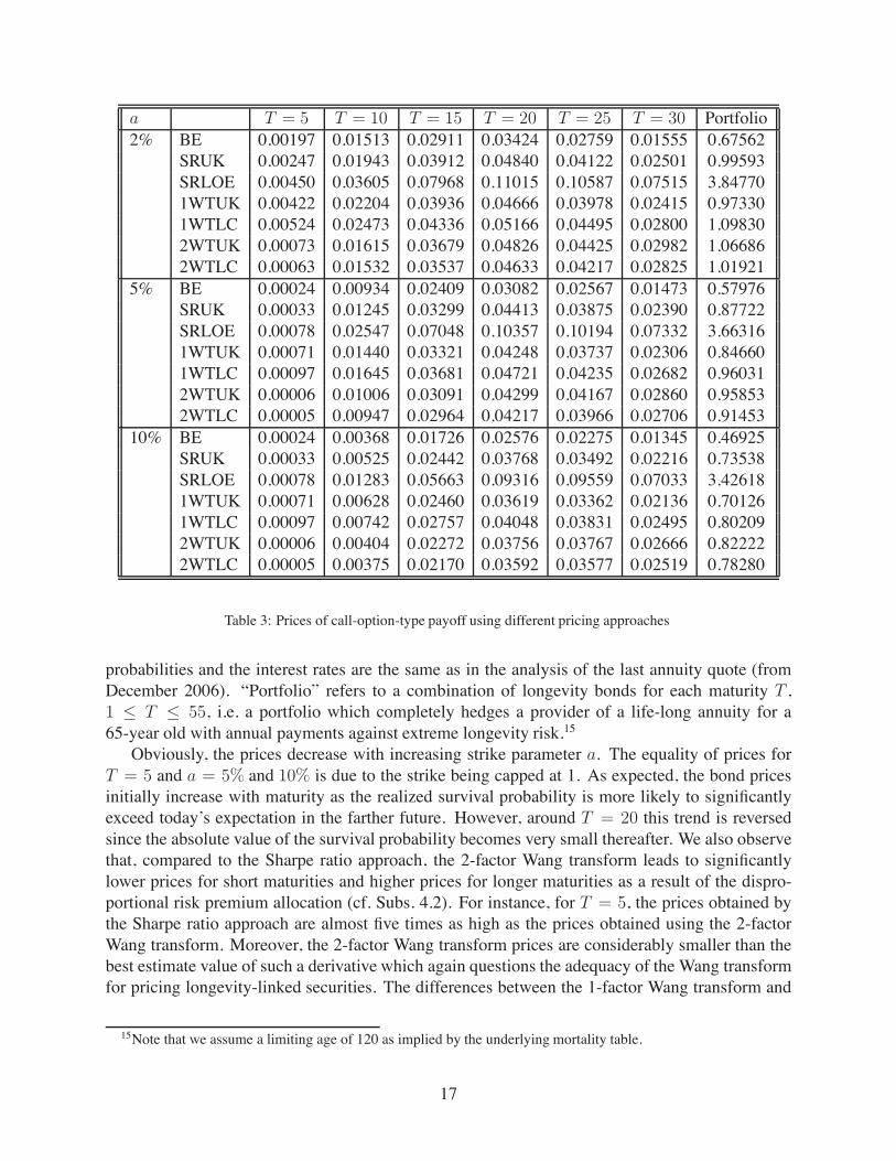
Within the setup introduced in Section 3, such a derivative can be priced by a Black-typeformula (see Bauer (2008)). One only needs to provide the volatility of mortality, the best esti-mate and the risk-adjusted T -year survival probability for an x0-year old today, and the price of azero-coupon bond with maturity T . In Table 3, prices of this option-type longevity derivative arepresented for a 65-year old in December 2006, the seven pricing methods defined in Subsection4.1, and various combinations of maturity T and strike parameter a. The best estimate survival

14This derivative has already been introduced in Bauer (2008) and similar payoff structures can also be found in,e.g., Blake et al. (2006a) or Lin and Cox (2005).

16

a T = 5 T = 10 T = 15 T = 20 T = 25 T = 30 Portfolio2% BE 0.00197 0.01513 0.02911 0.03424 0.02759 0.01555 0.67562

SRUK 0.00247 0.01943 0.03912 0.04840 0.04122 0.02501 0.99593SRLOE 0.00450 0.03605 0.07968 0.11015 0.10587 0.07515 3.847701WTUK 0.00422 0.02204 0.03936 0.04666 0.03978 0.02415 0.973301WTLC 0.00524 0.02473 0.04336 0.05166 0.04495 0.02800 1.098302WTUK 0.00073 0.01615 0.03679 0.04826 0.04425 0.02982 1.066862WTLC 0.00063 0.01532 0.03537 0.04633 0.04217 0.02825 1.01921

5% BE 0.00024 0.00934 0.02409 0.03082 0.02567 0.01473 0.57976SRUK 0.00033 0.01245 0.03299 0.04413 0.03875 0.02390 0.87722SRLOE 0.00078 0.02547 0.07048 0.10357 0.10194 0.07332 3.663161WTUK 0.00071 0.01440 0.03321 0.04248 0.03737 0.02306 0.846601WTLC 0.00097 0.01645 0.03681 0.04721 0.04235 0.02682 0.960312WTUK 0.00006 0.01006 0.03091 0.04299 0.04167 0.02860 0.958532WTLC 0.00005 0.00947 0.02964 0.04217 0.03966 0.02706 0.91453

10% BE 0.00024 0.00368 0.01726 0.02576 0.02275 0.01345 0.46925SRUK 0.00033 0.00525 0.02442 0.03768 0.03492 0.02216 0.73538SRLOE 0.00078 0.01283 0.05663 0.09316 0.09559 0.07033 3.426181WTUK 0.00071 0.00628 0.02460 0.03619 0.03362 0.02136 0.701261WTLC 0.00097 0.00742 0.02757 0.04048 0.03831 0.02495 0.802092WTUK 0.00006 0.00404 0.02272 0.03756 0.03767 0.02666 0.822222WTLC 0.00005 0.00375 0.02170 0.03592 0.03577 0.02519 0.78280

Table 3: Prices of call-option-type payoff using different pricing approaches

probabilities and the interest rates are the same as in the analysis of the last annuity quote (fromDecember 2006). “Portfolio” refers to a combination of longevity bonds for each maturity T ,1 " T " 55, i.e. a portfolio which completely hedges a provider of a life-long annuity for a65-year old with annual payments against extreme longevity risk.15

Obviously, the prices decrease with increasing strike parameter a. The equality of prices forT = 5 and a = 5% and 10% is due to the strike being capped at 1. As expected, the bond pricesinitially increase with maturity as the realized survival probability is more likely to significantlyexceed today’s expectation in the farther future. However, around T = 20 this trend is reversedsince the absolute value of the survival probability becomes very small thereafter. We also observethat, compared to the Sharpe ratio approach, the 2-factor Wang transform leads to significantlylower prices for short maturities and higher prices for longer maturities as a result of the dispro-portional risk premium allocation (cf. Subs. 4.2). For instance, for T = 5, the prices obtained bythe Sharpe ratio approach are almost five times as high as the prices obtained using the 2-factorWang transform. Moreover, the 2-factor Wang transform prices are considerably smaller than thebest estimate value of such a derivative which again questions the adequacy of the Wang transformfor pricing longevity-linked securities. The differences between the 1-factor Wang transform and

15Note that we assume a limiting age of 120 as implied by the underlying mortality table.

17

the Sharpe ratio approach are not quite as strong but still significant.In order to assess the question of “how good of a deal” this derivative is from the insurer’s

perspective, we compare the price of a portfolio of our option-type longevity derivatives with theprice of a life-long immediate annuity. The average price of the annuity paying £1 annually inadvance in December 2006 was £14.92. Hence, for a rather low strike parameter (a = 2%) and aSharpe ratio implied by UK pension annuities, an insurer would have to pay approximately 6.7%of the single premium for a full coverage against extreme longevity improvements. Since thecompany would hardly be exposed to longevity risk anymore while, at the same time, profitingfrom realized longevity improvements below today’s expectation, the price appears to be veryreasonable, particularly if the value is interpreted as the upper bound. In case the company iswilling to accept a larger portion of the risk, e.g. for a = 10%, the (maximal) cost for the hedgecan be reduced to approximately 4.9% of the single premium.

Moreover, an insurer could reduce the cost of longevity coverage by incorporating the com-pany’s mortality exposure from the sale of life insurance policies. This idea of compensatinglongevity risk by mortality risk is often referred to as natural hedging (see, e.g., Bayraktar andYoung (2007), Cox and Lin (2007), or Wetzel and Zwiesler (2008)). Although such a compen-sation is only partial since the age cohorts exposed to these risks are typically different and thematurities of annuities generally exceed those of life insurance policies, the number of longevity-linked securities necessary to reduce the longevity risk to a desired level can certainly be reduced.

6. Conclusion

The current paper analyzes and compares different approaches for pricing longevity-linkedsecurities. Milevsky et al. (2006) postulate that an issuer of such a security should be compensatedfor taking longevity risk according to a pre-specified instantaneous Sharpe ratio. Lin and Cox(2005, 2008), on the other hand, apply the Wang transform to best estimate death probabilities inorder to account for a risk premium.

However, as explained in detail in Section 3, the risk premium implied by theWang transform isnot consistent – arbitrage opportunities may arise as soon as multiple securities based on differentcohorts are traded. Even if only one security is considered, the disproportional risk premiumallocation contests the adequacy of an application of the Wang transform for pricing longevityderivatives (cf. Subs. 4.2 and Sec. 5).

Moreover, we discuss the derivation of an adequate market price of longevity risk, i.e. a Sharperatio or Wang transform parameters in our case. Milevsky et al. (2005) do not address this questionbut Loeys et al. (2007) propose to adopt a Sharpe ratio from equity markets. We believe that thisapproach is not appropriate since peculiarities of equity markets may not be present in the longevitymarket. In contrast, Lin and Cox (2005, 2008) obtain their Wang transform parameters from USannuity quotes which is more sound from our point of view.

We compare the different pricing approaches based on UK data. In particular, we derive atime series for the market price of risk within market annuity quotes and analyze the relationshipto interest rates and the stock market. We find considerable correlations indicating that the inde-pendence assumption of the risk-adjusted mortality evolution and the development of the financialmarket may not be adequate.

We then apply the different approaches to assess the first announced – but never issued –longevity bond, the so-called EIB/BNP-Bond. For each of the considered “risk-adjusting” meth-

18

ods, the price exceeds the £540mn quoted by BNP, i.e. the Bond appears to have been a rather“good deal”. Even if the “risk-adjusted” prices are interpreted as upper bounds for the EIB/BNP-Bond’s fair value with the best estimate value as the lower bound, the price quoted by BNP appearsat least reasonably fair. Consequently, there must have been other reasons for its failure, for exam-ple the financial engineering.

We propose a differently designed and potentially more suitable security, namely an option-type longevity derivative. Such a security allows an insurer to keep the “equity tranche” of thelongevity risk in the company’s own books. We derive prices for derivatives of this kind based onthe different methods and compare the results. All in all, we believe that such option-type longevityderivatives could become successful tools for securitizing longevity risk.

References

Azzopardi, M., 2005. The Longevity Bond. Presentation at the First International Conference onLongevity Risk and Capital Market Solutions, 2005.

Barro, R.J., 2006. Rare Disasters and Asset Markets in the Twentieth Century. The QuarterlyJournal of Economics, 121: 823–866.

Bauer, D., 2008. Stochastic Mortality Modeling and Securitization of Mortality Risk. ifa-Verlag,Ulm (Germany).

Bauer, D., Borger, M., Ruß, J., Zwiesler, H.-J., 2008. The Volatility of Mortality. Asia-PacificJournal of Risk and Insurance, 3: 184–211.

Bauer, D., Weber, F., 2008. Assessing Investment and Longevity Risks within Immediate Annu-ities. Asia-Pacific Journal of Risk and Insurance, 3: 90–112.

Bayraktar, E., Milevsky, M.A., Promislow, S.D., Young, V.R., 2008. Valuation of Mortality Riskvia the Instantaneous Sharpe Ratio: Applications to Life Annuities. To appear in: Journal ofEconomic Dynamics and Control.

Bayraktar, E., Young, V.R., 2007. Hedging life insurance with pure endowments. Insurance:Mathematics and Economics, 40: 435–444.

Bayraktar, E., Young, V.R., 2008. Pricing Options in Incomplete Equity Markets via the Instanta-neous Sharpe Ratio. Annals of Finance, 4: 399–429.

Biffis, E., 2005. Affine processes for dynamic mortality and actuarial valuation. Insurance: Math-ematics and Economics, 37: 443–468.

Bjork, T., 1999. Arbitrage Theory in Continuous Time. Oxford University Press, Oxford, UK.

Blake, D., Burrows, W., 2001. Survivor Bonds: Helping to Hedge Mortality Risk. The Journal ofRisk and Insurance, 68: 339–348.

Blake, D., Cairns, A.J.G., Dowd, K., 2006a. Living with mortality: longevity bonds and othermortality-linked securities. British Actuarial Journal, 12: 153–197.

19

Blake, D., Cairns, A.J.G., Dowd, K., MacMinn, R., 2006b. Longevity Bonds: Financial Engineer-ing, Valuation and Hedging. The Journal of Risk and Insurance, 73: 647–672.

Bowers, N.L., Gerber, H.U., Hickman, J.C, Jones, D.A., Nesbitt, C.J., 1997. Actuarial Mathemat-ics. 2nd Edition. The Society of Actuaries, Schaumburg, Il, USA.

Brown, J.R., Orszag, P.R., 2006. The Political Economy of Government Issued Longevity Bonds.The Journal of Risk and Insurance, 73: 611–631.

Cairns, A.J.G., Blake, D., Dawson, P., Dowd, K., 2005. Pricing the Risk on Longevity Bonds. Lifeand Pensions, October 2005: 41–44.

Cairns, A.J.G., Blake, D., Dowd, K., 2006a. A Two-Factor Model for Stochastic Mortality withParameter Uncertainty: Theory and Calibration. The Journal of Risk and Insurance, 73: 687–718.

Cairns, A.J.G., Blake, D., Dowd, K., 2006b. Pricing Death: Frameworks for the Valuation andSecuritization of Mortality Risk. ASTIN Bulletin, 36: 79–120.

Cowley, A., Cummins, J.D., 2005. Securitization of Life Insurance Assets and Liabilities. TheJournal of Risk and Insurance, 72: 193–226.

Cox, S.H., Lin, Y., 2007. Natural Hedging of Life and Annuity Mortality Risks. North AmericanActuarial Journal, 11: 1–15.

Dahl, M., 2004. Stochastic mortality in life insurance: market reserves and mortality-linked insur-ance contracts. Insurance: Mathematics and Economics, 35: 113–136.

Denuit, M., Devolder, P., Goderniaux, A.-C., 2007. Securitization of Longevity Risk: PricingSurvivor Bonds with Wang Transform in the Lee-Carter Framework. The Journal of Risk andInsurance, 74: 87–113.

Dowd, K., Blake, D., Cairns, A.J.G., Dawson, P., 2006. Survivor Swaps. The Journal of Risk andInsurance, 73: 1–17.

Duffie, D., Skiadas, C., 1994. Continuous-time security pricing: A utility gradient approach.Journal of Mathematical Economics, 23: 107–131.

Finkelstein, A., Poterba, J., 2002. Selection Effects in the United Kingdom Individual AnnuitiesMarket. Economic Journal, 112: 28–50.

Friedberg, L., Webb, A., 2007. Life is Cheap: Using Mortality Bonds to Hedge Aggregate Mor-tality Risk. The B.E. Journal of Economic Analysis & Policy, 7.

Grimshaw, D., 2007. Mortality Projections. Presentation at the Current Issues in Life Assuranceseminar, 2007.

Harrison, M., Kreps, D., 1979. Martingales and arbitrage in multiperiod security markets. Journalof Economic Theory, 20: 381–408.

20

Heath, D., Jarrow, R., Morton, R., 1992. Bond pricing and the term structure of interest rates: Anew methodology for contingent claim valuation. Econometrica, 60: 77–105.

Karatzas, I., Shreve, S.E., 1991. Brownian Motion and Stochastic Calculus. Graduate Texts inMathematics, 113. Springer, New York, NY (USA).

Kling, A., Richter, A., Ruß, J., 2008. Tax Incentives for Annuitization: Direct and Indirect Effects.Working Paper, Ulm University.

Lin, Y., Cox, S.H., 2005. Securitization of Mortality Risks in Life Annuities. The Journal of Riskand Insurance, 72: 227–252.

Lin, Y., Cox, S.H., 2008. Securitization of Catastrophe Mortality Risks. Insurance: Mathematicsand Economics, 42: 628–637.

Loeys, J., Panigirtzoglou, N., Ribeiro, R.M., 2007. Longevity: a market in the making. WorkingPaper, JPMorgan Global Market Strategy.

Loisel, S., Serant, D., 2007. In the Core of Longevity Risk: Dependence in Stochastic MortalityModels and Cut-Offs in Prices of Longevity Swaps. Working Paper, Universite Lyon 1.

Mehra, R., Prescott, E.C., 1985. The Equity Premium: A Puzzle. Journal of Monetary Economics,15: 145–161.

Milevsky, M.A., Promislow, S.D., 2001. Mortality Derivatives and the Option to Annuitize. Insur-ance: Mathematics and Economics, 29: 299–318.

Milevsky, M.A., Promislow, S.D., Young, V.R., 2005. Financial Valuation of Mortality Risk viathe Instantaneous Sharpe Ratio. Working Paper, York University and University of Michigan.

Milevsky, M.A., Promislow, S.D., Young, V.R., 2006. Killing the Law of Large Numbers: Mortal-ity Risk Premiums and the Sharpe Ratio. The Journal of Risk and Insurance, 73: 673–686.

Milevsky, M.A., Young, V.R., 2007. The timing of annuitization: Investment dominance andmortality risk. Insurance: Mathematics and Economics, 40: 135–144.

Miltersen, K.R., Persson, S.A., 2005. Is mortality dead? Stochastic force of mortality determinedby no arbitrage. Working Paper, University of Bergen.

Mitchell, O.S., Poterba, J.M., Warshawsky, M.J., Brown, J.R., 1999. New evidence on the money’sworth of individual annuities. American Economic Review, 89: 1299–1318.

Pelsser, A., 2008. On the Applicability of the Wang Transform for Pricing Financial Risks. ASTINBulletin, 38: 171–181.

Polyanin, A.D., Manzhirov, A.V., 1999. Handbuch der Integralgleichungen: exakte Losungen.Spektrum, Heidelberg.

Wang, S., 2002. A Universal Framework for Pricing Financial and Insurance Risks. ASTINBulletin, 32: 213–234.

21

Weale, M., Van de Ven, J., 2006. A General EquilibriumAnalysis of Annuity Rates in the Presenceof Aggregate Mortality Risk. National Institute of Economic and Social Research, DiscussionPaper 282.

Weitzman, M.L., 2007. Subjective Expectations and Asset-Return Puzzles. American EconomicReview, 97: 1102–1130.

Wetzel, C., Zwiesler, H.J., 2008. Das Vorhersagerisiko der Sterblichkeitsentwicklung - Kann esdurch eine geeignete Portfoliozusammensetzung minimiert werden? Blatter der DGVFM, 29:73–107.

Appendix

A. The Gaussian Mortality Model from Bauer et al. (2008)

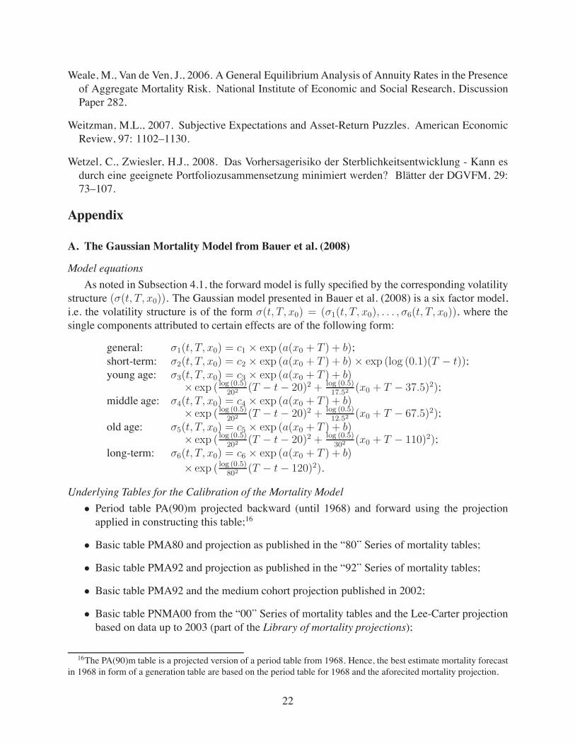
Model equationsAs noted in Subsection 4.1, the forward model is fully specified by the corresponding volatility

structure ($(t, T, x0)). The Gaussian model presented in Bauer et al. (2008) is a six factor model,i.e. the volatility structure is of the form $(t, T, x0) = ($1(t, T, x0), . . . , $6(t, T, x0)), where thesingle components attributed to certain effects are of the following form:

general: $1(t, T, x0) = c1 & exp (a(x0 + T ) + b);short-term: $2(t, T, x0) = c2 & exp (a(x0 + T ) + b) & exp (log (0.1)(T ! t));young age: $3(t, T, x0) = c3 & exp (a(x0 + T ) + b)

& exp ( log (0.5)202 (T ! t ! 20)2 + log (0.5)

17.52 (x0 + T ! 37.5)2);middle age: $4(t, T, x0) = c4 & exp (a(x0 + T ) + b)

& exp ( log (0.5)202 (T ! t ! 20)2 + log (0.5)

12.52 (x0 + T ! 67.5)2);old age: $5(t, T, x0) = c5 & exp (a(x0 + T ) + b)

& exp ( log (0.5)202 (T ! t ! 20)2 + log (0.5)

302 (x0 + T ! 110)2);long-term: $6(t, T, x0) = c6 & exp (a(x0 + T ) + b)

& exp ( log (0.5)802 (T ! t ! 120)2).

Underlying Tables for the Calibration of the Mortality Model• Period table PA(90)m projected backward (until 1968) and forward using the projectionapplied in constructing this table;16

• Basic table PMA80 and projection as published in the “80” Series of mortality tables;

• Basic table PMA92 and projection as published in the “92” Series of mortality tables;

• Basic table PMA92 and the medium cohort projection published in 2002;

• Basic table PNMA00 from the “00” Series of mortality tables and the Lee-Carter projectionbased on data up to 2003 (part of the Library of mortality projections);

16The PA(90)m table is a projected version of a period table from 1968. Hence, the best estimate mortality forecastin 1968 in form of a generation table are based on the period table for 1968 and the aforecited mortality projection.

22

• Basic table PNMA00 from the “00” Series of mortality tables and the Lee-Carter projectionbased on data up to 2004 (part of the Library of mortality projections);

• Basic table PNMA00 from the “00” Series of mortality tables and the Lee-Carter projectionbased on data up to 2005 (part of the Library of mortality projections).

Calibration resultsAccording to the notation in Bauer et al. (2008), we deployed the data points

(T ! t, x0 + T ) ) {(0, 30), (0, 70), (0, 110), (30, 70), (30, 110), (90, 110)} .

Moreover, we chose the slope parameter of the correction term to be a = 0.9 since this is theaverage value over all tables of the slope parameter in Gompertz forms fitted to the cohort mortalityof a 20-year old in the respective basis years. The parameter b is chosen as -10. The resulting valuesfor the volatility parameters are:

Parameters c1 c2 c3 c4 c5 c6

0.007 0.287 0.144 0.284 0.021 0.058

23