On the performance of nonparametric specification tests in regression models

Computational Statistics & Data Analysis 42 (2003) 477–490www.elsevier.com/locate/csda

On the performance of nonparametricspeci%cation tests in regression models

Daniel Milesa , Juan Morab;∗aDepartamento de Econom �a Aplicada, Universidad de Vigo, Spain

bDepartamento de Fundamentos del An alisis Econ omico, Universidad de Alicante,Apartado de Correos 99, E-03080, Alicante, Spain

Received 1 December 2001; received in revised form 1 June 2002

Abstract

Some recently developed nonparametric speci%cation tests for regression models are describedin a uni%ed way. The common characteristic of these tests is that they are consistent against anyalternative hypothesis. The performance of the test statistics is compared by means of MonteCarlo simulations, analysing how heteroskedasticity, number of regressors and bandwidth selec-tion in1uence the results. The statistics which do not use a bandwidth perform slightly betterif the regression model has only one regressor; otherwise, some of the statistics which use abandwidth behave better if the bandwidth is chosen adequately. These statistics are applied totest the speci%cation of three commonly used Mincer-type wage equations with Uruguayan andSpanish data; all of them are rejected.c© 2002 Elsevier Science B.V. All rights reserved.

Keywords: Nonparametric speci%cation tests; Wage equations

1. Introduction

The usual approach for examining a relation among economic variables is to spec-ify a functional form depending on unknown parameters that are then estimated andtested using a data set. This approach, however, is problematic since economic theoryoften does not suggest such functional forms. At best it results in a list of potentialexplanatory variables. Further, if the chosen functional form does not properly capture

∗ Corresponding author. Tel.: +34-965903614; fax: +34-965903898.E-mail address: [email protected] (J. Mora).

0167-9473/03/$ - see front matter c© 2002 Elsevier Science B.V. All rights reserved.PII: S0167 -9473(02)00227 -X

mailto:[email protected]

478 D. Miles, J. Mora / Computational Statistics & Data Analysis 42 (2003) 477–490

the nature of the data, there is a danger of arriving at incorrect conclusions. More-over, most empirical studies do not test the assumed parametric speci%cation properlythrough the use of a general alternative hypothesis.

The %rst concern of this paper is to present newly developed, appropriate non-parametric speci%cation tests and to compare their performance with moderate samplesizes by means of simulations. Speci%cally, we are interested in analysing how band-width selection may aGect the behaviour of the statistics, how sensitive they are tothe homoskedasticity assumption, and to what extent the performance of the statisticsimproves when bootstrap critical values are used instead of asymptotic ones.

The second concern of this paper is to apply these procedures to study the appro-priateness of certain wage equations. Characterizing wage pro%les is a long-standingissue, given its key role in understanding poverty, internal migrations, wage inequality,the performance of earnings-based pension plans, the consequences of implementinguniversal educational programmes and so on (see Manski, 2000). The Mincer-typewage equation, which speci%es the logarithm of wage as a linear combination of yearsof schooling, experience, squared experience and other individual characteristics, isthe functional form that has been most commonly used to estimate expected earningspro%les. As Willis (1986) states, as an empirical tool “the Mincer earnings functionhas been one of the great success stories of modern labour economics”. In this paper,we analyse the validity of various Mincer-type wage equations using Uruguayan andSpanish data.

The remainder of the paper is structured as follows. Section 2 describes the teststatistics considered here. Section 3 presents the results of three Monte Carlo experi-ments. Section 4 describes Mincer-type wage equations, the data sets and the empiricalresults. Finally, in Section 5, the conclusions are presented.

2. Nonparametric tests for speci�cation of regression models

In this section, we present the basic ideas behind the nonparametric statistics recentlydeveloped to test the speci%cation of a regression model. Let (X; Y ) denote a Rd × Rrandom vector and assume that Y is integrable so that the regression function m(x) =E(Y |X = x), x∈Rd, is well de%ned. Parametric modelling assumes that m(·) belongsto a given family M = {m(·; �): �∈ ⊂ Rp}, i.e. m(x) = m(x; �0) for some “true”parameter value �0. Therefore, statistical inference based on M should be accompaniedby a test for H0: m(·)∈M versus the nonparametric alternative H1: m(·) �∈ M.

The procedures proposed in the literature for performing tests of this type can beclassi%ed into two groups: those that use a smoothing value (smoothing tests) andthose that do not (nonsmoothing tests). All of these procedures require the use ofa parametric estimator of m(x) under H0; the natural one is m(x; �), where � is anyroot-n-consistent estimator of �0, e.g. the nonlinear least-squares estimator under certainassumptions. The smoothing tests also require the use of a nonparametric estimator ofm(x); the most popular one is the Nadaraya–Watson estimator: mh(x) =

∑ni=1 K[(x −

Xi)=h]Yi=∑n

i=1 K[(x−Xi)=h], where {(Xi; Yi)}ni=1 are the observations, h is a smoothing

value (or bandwidth) and K(·) :Rd → R is a symmetric kernel function (hereafter,

D. Miles, J. Mora / Computational Statistics & Data Analysis 42 (2003) 477–490 479

0=0 is arbitrarily de%ned to be 0). The main advantage of the smoothing tests overthe nonsmoothing ones is that their null asymptotic distribution is known; their maindisadvantage is that their performance (size and power) depends, crucially, on thechoice of the smoothing value. We now brie1y describe the test statistics that will beconsidered here. In each case, we discuss how critical values can be obtained, assumingthat certain technical conditions, which we do not specify, are satis%ed. The wildbootstrap procedure which is sometimes required to obtain critical values is describedat the end of this section. Under H1, all of these statistics diverge to +∞, hence, thecritical region is always one sided.

The statistic proposed by Gozalo (1993) is based on the squared diGerence betweenthe parametric estimator and the Bierens–Nadaraya–Watson nonparametric estimator atL points {xl}L

l=1 in the support of X :

T (G)n = nhd

L∑l=1

[m(xl; �) − mh;�(xl)]2

vh(xl);

where mh;�(x) = [mh(x)− (h=s)rms(x)]=[1− (h=s)r], ms(x) is de%ned as mh(x) replacingh by s = hn(1−�)=(2r+d), � is any value in (0; 1), r is the order of the kernel function,vh(x)=cK V (x)={(1=nhd)

∑ni=1 K[(x−Xi)=h]}, cK =

∫K(u)2 du and V (x) is a consistent

estimator of Var(Y |X = x). If this conditional variance is assumed to be constant, it ispossible to use V (x) = n−1 ∑n

i=1 [Yi − mh(Xi)]2; but if no parametric form is assumedfor it, a sensible choice would be V (x)=

∑ni=1 K[(x−Xi)=h][Yi−mh(Xi)]2=

∑ni=1 K[(x−

Xi)=h]. The asymptotic null distribution of T (G)n is �2

L. This test statistic is only consis-tent if the regression function speci%ed under H0 and the true regression function arediGerent at xl for some l∈{1; : : : ; L}.

HQardle and Mammen (1993) base their statistic on the weighted squared diGerencebetween the Nadaraya–Watson estimator and a kernel-smoothed parametric estimator:

T (HM)n = nhd=2

∫[mh(x) − mh; �(x)]2�(x) dx;

where mh; �(x) =∑n

i=1 K[(x − Xi)=h]m(Xi; �)=∑n

i=1 K[(x − Xi)=h]; �(·) :Rd → R is aweight function, the range of integration is the support of X and the integral can benumerically approximated. The asymptotic null distribution of T (HM)

n is normal, but theauthors recommend computing critical values using a bootstrap procedure describedbelow. This test statistic is consistent against any alternative hypothesis.

The statistic proposed by Zheng (1996) can be viewed as a conditional moment teststatistic based on the following moment condition, which holds under the null hypo-thesis: E[UE(U |X )p(X )] = 0, where U =Y −m(X; �0) and p(·) is the density functionof X . This moment condition suggests basing the statistic on n−1 ∑n

i=1 U iE(Ui|Xi),where U i and E(Ui|Xi) are suitable estimates of Ui and E(Ui|Xi). Speci%cally, usingkernel smoothers and parametric residuals ei = Yi − m(Xi; �), the statistic they derivedis

T (Z)n =

∑ni=1 ei

∑nj=1; j �=i K[(Xi − Xj)=h]ej

(2∑n

i=1

∑nj=1; j �=i {K[(Xi − Xj)=h)]eiej}2)1=2

:


The asymptotic null distribution of T (Z)n is standard normal, and it is also consistent

against any alternative. Li and Wang (1998) have proven that the performance of T (Z)n

could be improved if critical values are obtained using a bootstrap procedure.The idea behind the statistic proposed by Ellison and Ellison (2000) is the same

as the one in Zheng (1996), but the sample analogue is constructed using normal-ized weights whose sum is one for each observation and, additionally, a %nite-samplecorrection term is included. When kernel weights are used, the statistic they proposebecomes

T (EE)n =

∑ni=1 ei

∑nj=1; j �=i Kh; ijej

(2∑n

i=1

∑nj=1; j �=i K2

h; ije2i e

2j )1=2

+1 + d

(2∑n

i=1

∑nj=1; j �=i K2

h; ij)1=2

;

where Kh; ij = 12 K[(Xi − Xj)=h]({∑n

l=1; l�=i K[(Xi − Xl)=h]}−1 + {∑nl=1; l�=j K[(Xj − Xl)=

h]}−1). The asymptotic null distribution of T (EE)n is standard normal; it is also consistent

against any alternative hypothesis.Horowitz and HQardle (1994) consider a slightly diGerent context from ours,

but their statistic can also be used to test our null and alternative hypotheses;here, we adapt their motivation and statistic to our context. Their statistic can beviewed as a conditional-moment test statistic, based on the moment conditionE{UE[U |m(X; �0)]w[m(X; �0)]}= 0, which holds under H0 for any nonnegative weightfunction w(·) :R → R. This moment condition suggests basing the statistic onn−1 ∑n

i=1 U i[Y i − m(Xi; �)], where U i and Yi are suitable estimates of Ui andE[Yi|m(Xi; �0)]. Using kernels, and after certain normalizations, the statistic derivedis

T (HH)n =

∑nj=1 ej[Y h;�; j − m(Xj; �)]w[m(Xj; �)]

{(2cK=nh)∑n

j=1 V2

j w[m(Xj; �)]2=ph; j}1=2;

where Y h;�; j = [Y h; j − (h=s)rY s; j]=[1− (h=s)r], Y h; j = (nhph;j)−1 ∑ni=1; i �=j K{[m(Xj; �)−

m(Xi; �)]=h}Yi, ph; j =(nh)−1 ∑ni=1; i �=j K{[m(Xj; �)−m(Xi; �)]=h}, Y s; j, ps; j are de%ned

as Y h; j, ph; j replacing h by s = hn(1−�)=(2r+d), and V j is a consistent estimator ofVar[Yj|m(Xj; �)]. If this conditional variance is assumed to be constant, it is possible touse V j =n−1 ∑n

i=1 (Yi− Y h;�; i)2; but if no parametric form is assumed for it, a sensiblechoice would be V j=(nhph;j)−1 ∑n

i=1; i �=j K{[m(Xj; �)−m(Xi; �)]=h}(Yi−Y h;�; i)2. Under

H0, T (HH)n converges to a standard normal distribution. The main advantage of T (HH)

n

over the other smoothing tests is that the nonparametric estimation that is made hasonly one explanatory variable; hence, the “curse of dimensionality” of nonparametricestimators is avoided and the statistic is expected to perform well, even with moderatesample sizes. The disadvantage of T (HH)

n is that, unlike all the other statistics describedhere, it is not consistent against all alternatives, but only against those for whichE({E[Y |m(X; �1)]−m(X; �1)}2w[m(X; �1)]) ¿ 0, where �1,is the probability limit of �.

The nonsmoothing tests base their statistics on empirical processes de%ned in sucha way that any deviation from the null hypothesis is detected. Bierens (1990)and Bierens and Ploberger (1997) suggest considering the empirical process Zn(t)=


n−1=2 ∑ni=1 ei!(t; Xi), for t ∈& ⊆ Rd and a smooth function !(·) : & × Rd → R, and

then using a functional of this process as the test statistic. If !(·) is chosen adequately,statistics constructed in this way can be viewed as conditional-moment test statisticsbased on an in%nite set of moment conditions; hence, they are consistent against allpossible alternatives. Here, we consider the Bierens statistic

∫Zn(t)2 dF(t), where F(·)

is the product of d standard normal distribution functions, !(t; X ) = exp[t′((X )] for asuitable function ((·) :Rd → Rd, and the range of integration is Rd. The statistic thusobtained is

T (B)n = n−1

n∑i=1

n∑j=1

eiej exp

[12

d∑l=1

(Zil + Zjl)2

];

where Zil is the lth component of Zi = ((Xi). Note that our choice of F(·) doesnot satisfy the requirement of compact support contained in Bierens and Ploberger(1997), but we follow the suggestion of Fan and Li (2000), who study this versionof the Bierens statistic and show that the asymptotic null distribution of T (B)

n can beapproximated by a bootstrap procedure.

Stute (1997) observes that H0 holds if and only if E[UI(X 6 t)] = 0 for all t ∈Rd,where I(·) is the indicator function. Hence, he proposes considering the empiricalprocess Rn(t) = n−1=2 ∑n

i=1 eiI(Xi6 t), and using a functional of this process as thetest statistic. Here, we consider the CramSer–von Mises statistic

T (S)n = n−1

n∑j=1

Rn(Xj)2 = n−2n∑

j=1

[n∑

i=1

eiI(Xi6Xj)

]2

;

whose asymptotic distribution, studied in detail in Stute (1997), can also be approxi-mated by bootstrap.

The bootstrap procedure which allows us to obtain critical values when using T (B)n

and T (S)n is usually referred to as “wild bootstrap” and works as follows: (i) generate

independent {e∗i }ni=1, where the distribution of e∗i is discrete with

Pr

{e∗i =

1 +√

52

ei

}=

5 −√5

10and Pr

{e∗i =

1 −√5

2ei

}=

5 +√

510

;

(ii) compute the bootstrap data {(X ∗i ; Y ∗

i )}ni=1, where X ∗

i =Xi and Y ∗i =m(Xi; �)+e∗i and,

with these data, the corresponding bootstrap statistic T ∗n ; (iii) repeat the process B times

to obtain {T ∗n; j}B

j=1, and reject H0 if Tn ¿T ∗n; (1−,), where T ∗

n; (1−,) is the (1−,) quantileof {T ∗

n; j}Bj=1 and , is the signi%cance level. This “wild bootstrap” procedure also allows

us to obtain critical values when using the statistic proposed by HQardle and Mammen(1993), but in this case, in the %rst step ei must be replaced by eh; i =Yi − mh(Xi). Thevalidity of the wild bootstrap procedure in this context has been studied in HQardle andMammen (1993), Li and Wang (1998), Stute et al. (1998) and Fan and Li (2000),among others.


3. Size and power of speci�cation tests: simulation results

We examine the behaviour of the speci%cation tests discussed above with a moderatesample size by means of some Monte Carlo experiments. We %rst generate n = 100independent observations as follows: Xi ∼ N(0; 1), Ui ∼ N(0; 1), Xi, and Ui indepen-dent, and Yi = m(Xi) + Ui, where

m(x) = x + c(x2 − 1)

and the value of c varies; henceforth, we will refer to this experiment as Model 1.To analyse if the statistics are sensitive to the assumption of homoscedasticity, wealso perform another experiment with the same characteristics as Model 1, but de%ningYi = m(Xi) + (1 + X 2

i =2)1=2Ui; this experiment will be referred to as Model 2. Inboth models, the null hypothesis we test is that the regression function is linear, i.e.E(Y |X = x) = �01 + �02x for some �0 = (�01; �02) in R2. Hence, H0 is true if and onlyif c = 0. To examine the performance of the tests when the number of regressors isgreater than one, we also perform an experiment with n=100 independent observationsas follows: Xi = (X1i ; X2i) ∼ bivariate normal distribution with mean (0; 0), var(X1i) =var(X2i)=1, cov(X1i ; X2i)=0, Ui ∼ N(0; 1), Xi and Ui independent, and Yi=m(X1i ; X2i)+Ui, where

m(x1; x2) = x1 + x2 + c(x21 − 1)(x2

2 − 1)

and the value of c varies; this experiment will be referred to as Model 3. As before,we also test the null hypothesis that the regression function is linear, i.e. E(Y |X1 =x1; X2 = x2) = �01 + �02x1 + �03x2 for some �0 = (�01; �02; �03) in R3, and again H0 istrue if and only if c = 0.

Parameter �0 is always estimated by least squares. In all univariate kernel estimationswe use the quartic kernel K(u) = 15

16 (1 − u2)2I(|u|6 1), so cK = 57 and r = 2. In

the multivariate estimations we use the product of quartic kernels. As regards thebandwidth, in the univariate estimations we use h = .SX n−1=5, where SX is the samplestandard deviation of the regressor. In the multivariate estimations, each regressor ispreviously divided by its sample standard deviation and we then use h = .n−1=(d+4).Suitable choices for . were selected from plots obtained with some samples, but in allof the cases we report the results for various . in order to see how this choice aGectsthe performance of the statistics.

The statistic T (G)n is computed in Models 1 and 2 using L = 3 points: −1, 0, 1; in

Model 3, L = 5 points are considered: (−1;−1), (−1; 1), (0; 0), (1;−1), (1; 1); in allcases, T (G)

n is computed with � = 0:5 and without assuming any parametric form forVar(Y |X = x). The statistic T (HM)

n is computed with �(x) = I(x∈ [ − 1:96; 1:96]) inModels 1 and 2, and �(x) = I(x∈ [ − 1:8; 1:8] × [ − 1:8; 1:8]) in Model 3; in all cases,the integral in T (HM)

n is approximated numerically. The statistic T (HH)n is computed with

�=0:5, w(·)=�(·) and without assuming any parametric form for Var[Yi|m(Xi; �)]. Assuggested in Bierens (1990), T (B)

n is computed with ((·)=(((·)1; : : : ; ((·)d), where forj=1; : : : ; d, we denote ((u)j ≡ arctan[(u− TX j)=SXj], and TX j and SXj are the sample meanand standard deviation of {Xji}n

i=1; in this case, additional experiments suggest that thechoice of !(·) and F(:) does not play a crucial role in the results. Finally, whenever


Table 1Proportion of rejections of H0 in Model 1 (, = 0:05)

Gozalo HQardle and Mammen Zheng

c . = 3:0 . = 3:5 . = 4:0 . = 3:0 . = 3:5 . = 4:0 . = 0:20 . = 0:40 . = 0:60

−0.5 0.909 0.930 0.935 0.991 0.991 0.993 0.522 0.707 0.797−0.4 0.723 0.754 0.768 0.955 0.960 0.956 0.313 0.447 0.548−0.3 0.455 0.485 0.525 0.799 0.812 0.809 0.176 0.261 0.312−0.2 0.202 0.228 0.290 0.480 0.488 0.486 0.091 0.105 0.105−0.1 0.082 0.093 0.144 0.178 0.171 0.159 0.053 0.045 0.044

0 0.052 0.059 0.099 0.064 0.057 0.050 0.034 0.037 0.0270.1 0.094 0.099 0.149 0.173 0.164 0.165 0.052 0.050 0.0480.2 0.213 0.231 0.286 0.475 0.483 0.481 0.094 0.113 0.1270.3 0.464 0.494 0.536 0.814 0.818 0.821 0.190 0.256 0.3030.4 0.746 0.782 0.797 0.937 0.946 0.947 0.319 0.451 0.5430.5 0.902 0.918 0.924 0.991 0.993 0.996 0.516 0.697 0.795

Ellison and Ellison Horowitz and HQardle Bierens Stute

c . = 3:0 . = 3:5 . = 4:0 . = 3:0 . = 3:5 . = 4:0

−0.5 0.995 0.993 0.993 0.977 0.974 0.969 0.997 0.987−0.4 0.972 0.969 0.964 0.919 0.918 0.910 0.988 0.934−0.3 0.835 0.827 0.816 0.726 0.726 0.714 0.902 0.763−0.2 0.494 0.472 0.458 0.379 0.370 0.350 0.624 0.444−0.1 0.164 0.132 0.109 0.118 0.089 0.076 0.216 0.150

0 0.082 0.052 0.031 0.077 0.048 0.027 0.048 0.0500.1 0.175 0.144 0.119 0.134 0.110 0.076 0.215 0.1600.2 0.502 0.474 0.446 0.372 0.354 0.340 0.626 0.4410.3 0.838 0.830 0.810 0.740 0.735 0.706 0.901 0.7770.4 0.976 0.972 0.968 0.927 0.925 0.919 0.988 0.9410.5 0.994 0.994 0.993 0.972 0.967 0.966 0.999 0.988

a bootstrap procedure is required we use B= 500 bootstrap replications. All the resultswe report are based on 2000 replications of the data-generating process, and have beencarried out using GAUSS programmes, which are available from the authors on request.

We %rst discuss the results obtained when there is only one regressor. In Tables 1and 2, we report the proportion of rejections of H0 in Models 1 and 2, respectively,when nominal signi%cance level is , = 0:05.

The %rst thing we observe in Table 1 is that the empirical size of the tests iscorrect in most cases: only T (Z)

n has an empirical size that is slightly below its nominalsize. Regarding the smoothing tests, the %rst conclusion to be drawn is that bandwidthdoes not seem to play a crucial role, as long as it is selected within a reasonablerange. This is probably not so surprising considering that a particular version of theBierens test corresponds to a kernel-regression-based test with a %xed bandwidth, asFan and Li (2000) have shown. In Model 1, assuming that the bandwidth has beencorrectly chosen, we observe that T (HM)

n and T (EE)n are the smoothing tests that perform




c . = 3:0 . = 3:5 . = 4:0 . = 3:0 . = 3:5 . = 4:0 . = 0:20 . = 0:40 . = 0:60

−0.5 0.862 0.873 0.874 0.939 0.941 0.942 0.402 0.566 0.652−0.4 0.671 0.689 0.703 0.821 0.821 0.816 0.242 0.350 0.418−0.3 0.450 0.457 0.478 0.608 0.611 0.606 0.146 0.217 0.263−0.2 0.241 0.250 0.283 0.356 0.349 0.340 0.084 0.088 0.094−0.1 0.117 0.127 0.170 0.175 0.165 0.153 0.060 0.049 0.053

0 0.090 0.097 0.124 0.091 0.086 0.079 0.041 0.039 0.0340.1 0.133 0.142 0.173 0.166 0.165 0.148 0.060 0.059 0.0530.2 0.247 0.254 0.294 0.351 0.347 0.330 0.090 0.107 0.1200.3 0.440 0.468 0.492 0.620 0.629 0.618 0.161 0.212 0.2480.4 0.704 0.726 0.724 0.807 0.808 0.804 0.253 0.348 0.4190.5 0.856 0.863 0.860 0.930 0.939 0.936 0.393 0.557 0.646


c . = 3:0 . = 3:5 . = 4:0 . = 3:0 . = 3:5 . = 4:0

−0.5 0.937 0.932 0.932 0.884 0.874 0.861 0.950 0.931−0.4 0.826 0.821 0.810 0.737 0.733 0.716 0.848 0.805−0.3 0.611 0.604 0.589 0.505 0.484 0.463 0.622 0.576−0.2 0.343 0.324 0.300 0.269 0.246 0.222 0.317 0.291−0.1 0.168 0.136 0.115 0.137 0.103 0.079 0.107 0.121

0 0.122 0.091 0.066 0.102 0.069 0.044 0.041 0.0550.1 0.184 0.148 0.123 0.150 0.116 0.095 0.115 0.1200.2 0.340 0.319 0.292 0.260 0.227 0.209 0.314 0.2960.3 0.607 0.586 0.569 0.507 0.483 0.465 0.613 0.5670.4 0.832 0.828 0.821 0.758 0.744 0.726 0.856 0.8160.5 0.927 0.923 0.922 0.866 0.865 0.854 0.946 0.920

better and that they both perform quite similarly. It is also possible to rank the othersmoothing statistics (from better to worse) as follows: T (HH)

n , T (G)n , T (Z)

n . Regardingthe nonsmoothing tests, according to their power functions, T (B)

n performs better thanT (S)

n ; in fact, T (B)n performs even better than any other smoothing test, whereas T (S)

n

performs similarly to T (HM)n and T (EE)

n . In the results of Model 2, we observe thatheteroskedasticity causes more sensitivity to bandwidth choice in smoothing tests, somedistortions in the size of the statistics (especially T (G)

n ) and, in all of the cases, adecrease in power. The statistics, however, continue to perform well, in the sense thatany departure from the null is detected and the empirical size is approximately correct.The conclusions drawn about the comparative performance of the statistics from theresults of Model 1 still hold.

In Table 3, we report the proportion of rejections of H0 in Model 3, which has tworegressors, when the nominal signi%cance level is , = 0:05.

In this table, we %rst observe that the performance of all the tests is worse here thanwhen there is only one regressor. The empirical size of the test is correct in all cases,




c . = 2:5 . = 3:0 . = 3:5 . = 3:0 . = 3:5 . = 4:0 . = 0:25 . = 0:50 . = 0:75

−0.5 0.661 0.692 0.709 0.786 0.644 0.476 0.095 0.221 0.340−0.4 0.553 0.559 0.600 0.616 0.475 0.363 0.064 0.120 0.186−0.3 0.389 0.384 0.444 0.412 0.286 0.197 0.057 0.093 0.116−0.2 0.288 0.295 0.359 0.251 0.182 0.134 0.046 0.058 0.069−0.1 0.221 0.204 0.274 0.131 0.091 0.058 0.035 0.039 0.035

0 0.180 0.176 0.245 0.098 0.059 0.034 0.038 0.049 0.0430.1 0.213 0.207 0.273 0.116 0.088 0.051 0.043 0.049 0.0440.2 0.277 0.273 0.334 0.247 0.194 0.133 0.042 0.060 0.0660.3 0.389 0.401 0.468 0.417 0.301 0.218 0.064 0.091 0.1160.4 0.539 0.555 0.587 0.608 0.460 0.354 0.076 0.146 0.1930.5 0.663 0.692 0.708 0.790 0.640 0.478 0.095 0.206 0.334


c . = 3:5 . = 4:0 . = 4:5 . = 4:0 . = 4:5 . = 5:0

−0.5 0.759 0.705 0.617 0.455 0.426 0.389 0.094 0.158−0.4 0.658 0.591 0.503 0.371 0.341 0.310 0.080 0.113−0.3 0.472 0.418 0.354 0.260 0.230 0.201 0.061 0.085−0.2 0.268 0.217 0.180 0.188 0.156 0.130 0.042 0.080−0.1 0.128 0.094 0.067 0.111 0.081 0.064 0.041 0.051

0 0.079 0.044 0.033 0.083 0.053 0.038 0.043 0.0430.1 0.116 0.081 0.057 0.114 0.089 0.063 0.034 0.0660.2 0.278 0.237 0.196 0.177 0.147 0.127 0.050 0.0700.3 0.468 0.391 0.325 0.258 0.225 0.201 0.058 0.1000.4 0.652 0.592 0.518 0.396 0.374 0.333 0.072 0.1180.5 0.766 0.709 0.625 0.467 0.439 0.406 0.097 0.149

except for Gozalo’s statistic. In this case, we carried out additional experiments to verifythat the sample size required to obtain the correct size is much greater. With regardto the other four smoothing statistics, the one that seems less sensitive to bandwidthchoice is Zheng’s statistic, which, however, is the one with the worst power properties.In fact, among smoothing statistics with the correct size, the ranking that is obtainedaccording to the power functions is similar as in Model 1, although T (EE)

n now performssomewhat better than T (HM)

n . The performance of the nonsmoothing tests in Model 3is dramatically worse than in Models 1 and 2; they both have approximately correctsize, but their power is clearly below that of the smoothing tests. With additionalexperiments, we veri%ed that the value of c required to obtain an empirical powerabove 0:5 with T (B)

n and T (S)n in Model 3 is approximately ±1.

To sum up, in the models with one regressor, the statistic T (B)n proposed by Bierens

(1990) is preferable, although the statistics T (S)n proposed by Stute (1997), T (EE)

n pro-posed by Ellison and Ellison (2000) and T (HM)

n proposed by HQardle and Mammen(1993) have similar properties; T (B)

n and T (S)n have the advantage of not requiring the


use of any smoothing value, although a bootstrap procedure is required to compute crit-ical values. In the model with two regressors, however, some of the smoothing statisticsperform better than the nonsmoothing ones; speci%cally, T (EE)

n is the one that yieldsthe best results, and it has the additional advantage of being able to be implementedwith critical values from the standard normal distribution.

4. Testing Mincer-type wage equations

In this section, we apply the statistics we analysed in the previous sections to testthree Mincer-type wage equation speci%cations, using Uruguayan and Spanish data. The%rst speci%cation we test is the traditional Mincer-type model, in which the logarithmof real hourly wages wi is regressed on a constant, years of schooling edi, years ofpotential work experience exi and its square:

wi = 01 + 02edi + 03exi + 04ex2i + ui:

This model is used in many papers on applied labour, including Buchinsky (1994) orDi Nardo et al. (1996). The second speci%cation adds cubic and quartic terms on yearsof potential work experience:

wi = 01 + 02edi + 03exi + 04ex2i + 05ex3

i + 06ex4i + ui:

Murphy and Welch (1992) indicate that this speci%cation provides a better %t than thetraditional model, which only includes exi and its square. Finally, we examine a thirdspeci%cation which is quite similar to the %rst one but which incorporates an interactionbetween education and potential work experience:

wi = 01 + 02edi + 03exi + 04ex2i + 05ediexi + ui:

The data on Uruguay was obtained from the Uruguayan Household Survey, from 1986through 1997 (Encuesta de Hogares, Instituto Nacional de EstadSVstica, Uruguay). Theframe of the survey is the Urugayan civilian population that lives in housing units, andis subdivided into two separate surveys: one for the metropolitan area of Montevideoand another for the rest of the country. We use the %rst of these surveys exclusively,since almost half of the Uruguayan population lives in Montevideo and two-thirds ofits economic activity takes place there. The sample is composed of males older than 13,which this is the legal working age in Uruguay. We only included individuals who hada positive salary in the month preceding the interview, and who had worked duringthe week before the interview, in either the private or the public sector. However,self-employed individuals, workers without salaries, entrepreneurs and those who hadnever worked were excluded (see Bucheli et al., 2000 for a detailed description ofthe survey). The Spanish data was obtained from the Encuesta de Estructura Salarial(1995). This survey gives detailed information on individuals, their earnings, theircharacteristics (age, education, etc.) as well as their employers’ characteristics (%rmsize, economic activity, type of wage bargaining, etc.). For a description of the sample,see CantSo et al. (2002). Here, we use the subsample of full-time male workers.

The variable of interest is the real hourly wage. For the Uruguayan data, it wasde%ned as the salary in the month before the interview, divided by four times the


hours worked during the week before the interview. Thus, we assume that the numberof hours worked for each individual week during the previous month is equal to thenumber of hours worked during the week before the interview. For the Spanish data,this was de%ned as the monthly salary divided by total hours worked in the month(see Di Nardo et al., 1996 for a justi%cation of the use of real hourly wages).

Before testing the wage speci%cations, we perform another Monte Carlo experimentto see how the test statistics behave with data that is similar to what will be used in theapplication. We generate n=500 independent observations, as follows: Xi =(X1i ; X2i) ∼bivariate normal distribution with mean (8:44; 25:52), var(X1i)=14:44, var(X2i)=149:8,cov(X1i ; X2i)=11:17, Ui ∼ N(0; 0:197), Xi and Ui independent, and Yi =m(X1i ; X2i)+Ui,where

m(x1; x2) = 5:66 + 0:814x1 + 0:043x2 − 0:000465x22 + c(x2

1 − 1)(x22 − 1)

and the value of c varies. This experiment will be referred to as Model 4. All of theparameters in this model have been obtained from the estimation of the %rst spec-i%cation for the Mincer-type model with Spanish data. We test the null hypothesisE(Y |X1 = x1; X2 = x2) = �01 + �02x1 + �03x2 + �04x2

2 for some �0 = (�01; �02; �03; �04)in R4. All estimations are performed with the same characteristics as in Model 3,except that in the Gozalo test the L = 5 points we consider are (8:44; 25:52) and(8:44 ± 14:141=2; 25:52 ± 149:81=2). In Table 4, we report the proportion of rejectionsof H0 in this model when the nominal signi%cance level is , = 0:05. These results arebased on 2000 replications of the data. When a bootstrap procedure is required B=200bootstrap replications are used. In this table we observe that all of the statistics haveapproximately the correct size, except for T (G)

n , which will therefore be excluded fromthe application. All of the statistics detect departures from the null, although the powerfunction obtained diGers greatly among statistics, what might have been expected con-sidering the results obtained for Model 3.

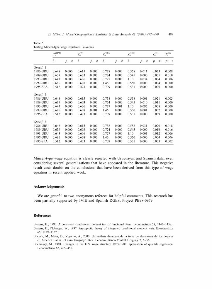
Finally, in Table 5 we report the p-value we obtain when we test each of thethree wage speci%cations. We use Uruguayan data for 1986, 1989, 1993 and 1997,and Spanish data for 1995. The number of Uruguayan observations in each year isn = 4509 for 1986, n = 5064 for 1989, n = 4920 for 1993 and n = 4847 for 1997. Forthe estimation with the Spanish data, we randomly selected a subsample of n = 5982observations (5% of the total sample). The estimations are performed with the samecharacteristics as those in Table 4, although, in this case, we use B = 1000 bootstrapreplications whenever required.

We observe in Table 5 that almost all of the speci%cations are rejected for all of thedata sets with the usual signi%cance levels. Note that this result is relatively robust,as we veri%ed that the statistics have the correct size in this context even with muchsmaller sample sizes. Additionally, the heteroskedasticity problem that could arise fromthe heterogeneity of the sample would cause a loss of power in the test, as seen inthe previous section, and therefore, does not aGect our conclusions. These results areof particular interest for applied work, as they imply that any conclusion drawn aboutthe earning pro%les based on the estimation of Mincer-type wage equations, like theones analyzed here, could be misleading. In the words of Manski (2000), “empirical%ndings are only as credible as the identifying assumptions imposed”.




c . = 1:0 . = 1:5 . = 2:0 . = 1:6 . = 1:8 . = 2:0 . = 0:20 . = 0:40 . = 0:60

−0.005 0.752 0.831 0.913 0.886 0.945 0.989 0.131 0.312 0.486−0.004 0.691 0.751 0.822 0.852 0.916 0.957 0.103 0.188 0.289−0.003 0.615 0.649 0.738 0.760 0.803 0.806 0.067 0.096 0.130−0.002 0.569 0.567 0.641 0.523 0.470 0.411 0.056 0.054 0.067−0.001 0.547 0.508 0.598 0.258 0.154 0.096 0.054 0.052 0.053

0 0.545 0.520 0.604 0.143 0.068 0.025 0.042 0.046 0.0360.001 0.548 0.556 0.641 0.222 0.140 0.081 0.049 0.051 0.0510.002 0.610 0.608 0.735 0.513 0.471 0.409 0.064 0.068 0.0760.003 0.654 0.702 0.797 0.761 0.807 0.799 0.064 0.103 0.1430.004 0.717 0.778 0.852 0.833 0.921 0.967 0.103 0.177 0.2840.005 0.775 0.850 0.923 0.851 0.941 0.988 0.134 0.291 0.510


c . = 4:0 . = 4:5 . = 5:0 . = 20 . = 25 . = 30

−0.005 1 1 1 0.188 0.129 0.084 0.731 1−0.004 0.999 1 1 0.181 0.110 0.067 0.610 1−0.003 0.983 0.985 0.986 0.167 0.102 0.061 0.382 0.983−0.002 0.743 0.757 0.766 0.129 0.079 0.047 0.206 0.754−0.001 0.239 0.220 0.224 0.093 0.058 0.032 0.078 0.214

0 0.088 0.058 0.047 0.069 0.047 0.029 0.029 0.0330.001 0.231 0.216 0.217 0.100 0.059 0.032 0.063 0.2270.002 0.729 0.749 0.764 0.180 0.102 0.049 0.154 0.7980.003 0.983 0.986 0.990 0.328 0.193 0.098 0.298 0.9900.004 1 1 1 0.547 0.358 0.195 0.416 10.005 1 1 1 0.732 0.517 0.321 0.765 1

5. Concluding remarks

The main objective of this study was to present, in a uni%ed way, the various non-parametric speci%cation tests for regression models that have recently appeared in theliterature, and to compare their performances in a common framework. Our results showthat when there is only one regressor, the nonsmoothing tests perform slightly betterthan the smoothing ones, especially the implementation we consider for the Bierensstatistic. Moreover, they have the obvious advantage that no bandwidth selection isrequired, though their implementation requires the use of a bootstrap procedure. Whenthe number of regressors is greater than one, some of the smoothing tests we considerhere perform better. Speci%cally, the statistic proposed in Ellison and Ellison (2000)exhibits good properties in all of the models we have simulated, and it has the addi-tional advantage of being able to be implemented with critical values from the standardnormal distribution.

The second objective of this study was to emphasize the importance of testing para-metric assumptions in applied work. Speci%cally, we have shown that the well-known


Table 5Testing Mincer-type wage equations: p-values

T (HM)n T (Z)

n T (EE)n T (HH)

n T (B)n T (S)

n

h p − v h p − v h p − v h p − v p − v p − v

Specif. 11986-URU 0.648 0.000 0.615 0.000 0.738 0.000 0.558 0.011 0.023 0.0081989-URU 0.639 0.000 0.603 0.000 0.724 0.000 0.545 0.000 0.005 0.0101993-URU 0.643 0.000 0.606 0.000 0.727 0.000 1.10 0.034 0.004 0.0061997-URU 0.686 0.000 0.608 0.000 1.46 0.000 0.550 0.000 0.004 0.0001995-SPA 0.512 0.000 0.473 0.000 0.709 0.000 0.531 0.000 0.000 0.000



Mincer-type wage equation is clearly rejected with Uruguayan and Spanish data, evenconsidering several generalizations that have appeared in the literature. This negativeresult casts doubts on the conclusions that have been derived from this type of wageequation in recent applied work.

Acknowledgements

We are grateful to two anonymous referees for helpful comments. This research hasbeen partially supported by IVIE and Spanish DGES, Project PB98-0979.

References

Bierens, H., 1990. A consistent conditional moment test of functional form. Econometrica 58, 1443–1458.Bierens, H., Ploberger, W., 1997. Asymptotic theory of integrated conditional moment tests. Econometrica

65, 1129–1152.Bucheli, M., Miles, D., Vigorito, A., 2000. Un anSalisis dinSamico de la toma de decisiones de los hogares

en AmSerica Latina: el caso Uruguayo. Rev. Econom. Banco Central Uruguay 7, 5–56.Buchinsky, M., 1994. Changes in the U.S. wage structure 1963–1987: application of quantile regression.

Econometrica 62, 405–458.


CantSo, O., Cardoso, A.R., Jimeno, J.F., 2002. Earnings inequality in Spain and Portugal: contrasts andsimilarities. In: Cohen, D., Piketty, T., Saint-Paul, G. (Eds.), The New Economics of Rising Inequalities.Oxford University Press, Oxford, forthcoming.

Di Nardo, J., Fortin, N., Lemieux, T., 1996. Labor market institutions and the distribution of wages: asemi-parametric approach. Econometrica 64, 1001–1044.

Ellison, G., Ellison, S.F., 2000. A simple framework for nonparametric speci%cation testing. J. Econometrics96, 1–23.

Fan, Y., Li, Q., 2000. Consistent model speci%cation tests: kernel-based tests versus Bierens’ ICM Tests.Econometric Theory 16, 1016–1041.

Gozalo, P., 1993. A consistent model speci%cation test for nonparametric estimation of regression functionmodels. Econometric Theory 9, 451–477.

HQardle, W., Mammen, E., 1993. Comparing nonparametric versus parametric regression %ts. Ann. Statist.21, 1926–1947.

Horowitz, J., HQardle, W., 1994. Testing a parametric model against a semi-parametric alternative. EconometricTheory 10, 821–848.

Li, Q., Wang, S., 1998. A simple consistent bootstrap test for a parametric regression function. J.Econometrics 87, 145–165.

Manski, C., 2000. Economic analysis of social interactions. J. Econom. Perspect. 14, 115–136.Murphy, W., Welch, G., 1992. The structure of wages. Quart. J. Econom. 107, 285–326.Stute, W., 1997. Nonparametric model checks for regression. Ann. Statist. 25, 613–641.Stute, W., GonzSalez-Manteiga, W., Presedo-Quindimil, M., 1998. Bootstrap approximations in model checks

for regression. J. Amer. Statist. Assoc. 93, 141–149.Willis, R., 1986. Wage determinants: a survey and reinterpretation of human capital earnings functions. In:

Ashenfelter, O., Layard, R. (Eds.), Handbook of Labor Economics, Vol. 1. North-Holland, Amsterdam,pp. 525–602.

Zheng, J., 1996. A consistent test of functional form via non-parametric estimation techniques. J.Econometrics 75, 263–289.

On the performance of nonparametric specification tests in regression models

Documents

Transcript of On the performance of nonparametric specification tests in regression models