On the One-Dimensional Modeling of Vertical Upward Bubbly Flow
11
Research Article On the One-Dimensional Modeling of Vertical Upward Bubbly Flow C. Peña-Monferrer, 1,2 C. Gómez-Zarzuela, 3 S. Chiva , 1 R. Miró, 3 G. Verdú, 3 and J. L. Muñoz-Cobo 2 1 Department of Mechanical Engineering and Construction, Universitat Jaume I, Campus del Riu Sec, 12080 Castell´ o de la Plana, Spain 2 Institute for Energy Engineering, Universitat Polit` ecnica de Val` encia, Cam´ ı de Vera, s/n, 46022 Val` encia, Spain 3 Research Institute for Industrial, Radiophysical and Environmental Safety, Universitat Polit` ecnica de Val` encia, Cam´ ı de Vera, s/n, 46022 Val` encia, Spain Correspondence should be addressed to S. Chiva; [email protected] Received 27 July 2017; Accepted 6 December 2017; Published 16 January 2018 Academic Editor: Tomasz Kozlowski Copyright © 2018 C. Pe˜ na-Monferrer et al. is is an open access article distributed under the Creative Commons Attribution License, which permits unrestricted use, distribution, and reproduction in any medium, provided the original work is properly cited. e one-dimensional two-fluid model approach has been traditionally used in thermal-hydraulics codes for the analysis of transients and accidents in water–cooled nuclear power plants. is paper investigates the performance of RELAP5/MOD3 predicting vertical upward bubbly flow at low velocity conditions. For bubbly flow and vertical pipes, this code applies the driſt- velocity approach, showing important discrepancies with the experiments compared. en, we use a classical formulation of the drag coefficient approach to evaluate the performance of both approaches. is is based on the critical Weber criteria and includes several assumptions for the calculation of the interfacial area and bubble size that are evaluated in this work. A more accurate drag coefficient approach is proposed and implemented in RELAP5/MOD3. Instead of using the Weber criteria, the bubble size distribution is directly considered. is allows the calculation of the interfacial area directly from the definition of Sauter mean diameter of a distribution. e results show that only the proposed approach was able to predict all the flow characteristics, in particular the bubble size and interfacial area concentration. Finally, the computational results are analyzed and validated with cross-section area average measurements of void fraction, dispersed phase velocity, bubble size, and interfacial area concentration. 1. Introduction Two-phase flow phenomena have been an object of study during several decades with a great impact in nuclear field. From the reactor to the turbines, one can find a wide variety of systems where two-phase flow plays a main role: BWR core, secondary loop, or reactor heat removal system (RHRS) are examples of two-phase flow components. In such cases, two-phase flow is present in normal operating conditions, but also in specific situations, like instabilities events, loss- of-coolant accidents, or refueling. e previous cases imply different conditions of pressure, temperature, or mass flow. is broad range of situations is considered in one- dimensional thermal-hydraulics codes to set the appropriate flow regime in each situation. ey are based on the two-fluid model [1], where averaged Navier-Stokes equations are solved for each phase including momentum, energy, and continuity equations. en, one can account for the interaction terms between phases, to consider the mass transfer, momentum, and energy at the interface. e interfacial momentum term differs depending on which flow regime is working. e proper regime is selected according to a flow regime map and the velocities of each phase. Different flow regime maps have been proposed by different authors [2, 3]. is paper investigates the performance of RELAP5/MOD3 predicting the results of experiments in a vertical upward bubbly flow for low velocity conditions. Bubbly flow at those conditions can be found in pressurizers, reactor pools, or refueling operations. To investigate in depth the bubbly flow behavior and the one-dimensional modeling, we perform experiments Hindawi Science and Technology of Nuclear Installations Volume 2018, Article ID 2153019, 10 pages https://doi.org/10.1155/2018/2153019
Transcript of On the One-Dimensional Modeling of Vertical Upward Bubbly Flow

Research ArticleOn the One-Dimensional Modeling of VerticalUpward Bubbly Flow
C Pentildea-Monferrer12 C Goacutemez-Zarzuela3 S Chiva 1 R Miroacute3
G Verduacute3 and J L Muntildeoz-Cobo2
1Department ofMechanical Engineering and Construction Universitat Jaume I Campus del Riu Sec 12080 Castello de la Plana Spain2Institute for Energy Engineering Universitat Politecnica de Valencia Camı de Vera sn 46022 Valencia Spain3Research Institute for Industrial Radiophysical and Environmental Safety Universitat Politecnica de ValenciaCamı de Vera sn 46022 Valencia Spain
Correspondence should be addressed to S Chiva schivaemcujies
Received 27 July 2017 Accepted 6 December 2017 Published 16 January 2018
Academic Editor Tomasz Kozlowski
Copyright copy 2018 C Pena-Monferrer et al This is an open access article distributed under the Creative Commons AttributionLicense which permits unrestricted use distribution and reproduction in any medium provided the original work is properlycited
The one-dimensional two-fluid model approach has been traditionally used in thermal-hydraulics codes for the analysis oftransients and accidents in waterndashcooled nuclear power plants This paper investigates the performance of RELAP5MOD3predicting vertical upward bubbly flow at low velocity conditions For bubbly flow and vertical pipes this code applies the drift-velocity approach showing important discrepancies with the experiments compared Then we use a classical formulation of thedrag coefficient approach to evaluate the performance of both approaches This is based on the critical Weber criteria and includesseveral assumptions for the calculation of the interfacial area and bubble size that are evaluated in this work A more accuratedrag coefficient approach is proposed and implemented in RELAP5MOD3 Instead of using the Weber criteria the bubble sizedistribution is directly considered This allows the calculation of the interfacial area directly from the definition of Sauter meandiameter of a distribution The results show that only the proposed approach was able to predict all the flow characteristics inparticular the bubble size and interfacial area concentration Finally the computational results are analyzed and validated withcross-section area average measurements of void fraction dispersed phase velocity bubble size and interfacial area concentration
1 Introduction
Two-phase flow phenomena have been an object of studyduring several decades with a great impact in nuclear fieldFrom the reactor to the turbines one can find a wide varietyof systems where two-phase flow plays a main role BWRcore secondary loop or reactor heat removal system (RHRS)are examples of two-phase flow components In such casestwo-phase flow is present in normal operating conditionsbut also in specific situations like instabilities events loss-of-coolant accidents or refueling The previous cases implydifferent conditions of pressure temperature or mass flow
This broad range of situations is considered in one-dimensional thermal-hydraulics codes to set the appropriateflow regime in each situationThey are based on the two-fluid
model [1] where averagedNavier-Stokes equations are solvedfor each phase including momentum energy and continuityequations Then one can account for the interaction termsbetween phases to consider the mass transfer momentumand energy at the interface The interfacial momentum termdiffers depending on which flow regime is working Theproper regime is selected according to a flow regime mapand the velocities of each phase Different flow regime mapshave been proposed by different authors [2 3] This paperinvestigates the performance of RELAP5MOD3 predictingthe results of experiments in a vertical upward bubbly flowfor low velocity conditions Bubbly flow at those conditionscan be found in pressurizers reactor pools or refuelingoperations To investigate in depth the bubbly flow behaviorand the one-dimensional modeling we perform experiments
HindawiScience and Technology of Nuclear InstallationsVolume 2018 Article ID 2153019 10 pageshttpsdoiorg10115520182153019
2 Science and Technology of Nuclear Installations
RELAP5MOD3
Drift-velocity approach (DVA)Drag coefficient approach
Critical Weber criteria (DCA)
Default model
Original model
Proposed modelBubble size distribution (DClowast)
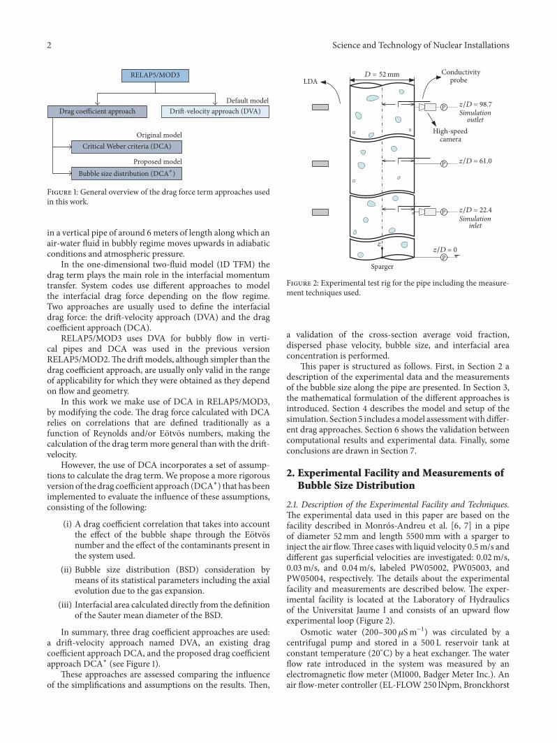
Figure 1 General overview of the drag force term approaches usedin this work
in a vertical pipe of around 6meters of length along which anair-water fluid in bubbly regime moves upwards in adiabaticconditions and atmospheric pressure
In the one-dimensional two-fluid model (1D TFM) thedrag term plays the main role in the interfacial momentumtransfer System codes use different approaches to modelthe interfacial drag force depending on the flow regimeTwo approaches are usually used to define the interfacialdrag force the drift-velocity approach (DVA) and the dragcoefficient approach (DCA)
RELAP5MOD3 uses DVA for bubbly flow in verti-cal pipes and DCA was used in the previous versionRELAP5MOD2The driftmodels although simpler than thedrag coefficient approach are usually only valid in the rangeof applicability for which they were obtained as they dependon flow and geometry
In this work we make use of DCA in RELAP5MOD3by modifying the code The drag force calculated with DCArelies on correlations that are defined traditionally as afunction of Reynolds andor Eotvos numbers making thecalculation of the drag termmore general than with the drift-velocity
However the use of DCA incorporates a set of assump-tions to calculate the drag term We propose a more rigorousversion of the drag coefficient approach (DCAlowast) that has beenimplemented to evaluate the influence of these assumptionsconsisting of the following
(i) A drag coefficient correlation that takes into accountthe effect of the bubble shape through the Eotvosnumber and the effect of the contaminants present inthe system used
(ii) Bubble size distribution (BSD) consideration bymeans of its statistical parameters including the axialevolution due to the gas expansion
(iii) Interfacial area calculated directly from the definitionof the Sauter mean diameter of the BSD
In summary three drag coefficient approaches are useda drift-velocity approach named DVA an existing dragcoefficient approach DCA and the proposed drag coefficientapproach DCAlowast (see Figure 1)
These approaches are assessed comparing the influenceof the simplifications and assumptions on the results Then
z
Conductivityprobe
Sparger
zD = 0
zD = 224
zD = 987
zD = 610
LDA
P
P
P
P
Simulationinlet
Simulationoutlet
High-speedcamera
D = 52mm
Figure 2 Experimental test rig for the pipe including the measure-ment techniques used
a validation of the cross-section average void fractiondispersed phase velocity bubble size and interfacial areaconcentration is performed
This paper is structured as follows First in Section 2 adescription of the experimental data and the measurementsof the bubble size along the pipe are presented In Section 3the mathematical formulation of the different approaches isintroduced Section 4 describes the model and setup of thesimulation Section 5 includes amodel assessmentwith differ-ent drag approaches Section 6 shows the validation betweencomputational results and experimental data Finally someconclusions are drawn in Section 7
2 Experimental Facility and Measurements ofBubble Size Distribution
21 Description of the Experimental Facility and TechniquesThe experimental data used in this paper are based on thefacility described in Monros-Andreu et al [6 7] in a pipeof diameter 52mm and length 5500mm with a sparger toinject the air flowThree cases with liquid velocity 05ms anddifferent gas superficial velocities are investigated 002ms003ms and 004ms labeled PW05002 PW05003 andPW05004 respectively The details about the experimentalfacility and measurements are described below The exper-imental facility is located at the Laboratory of Hydraulicsof the Universitat Jaume I and consists of an upward flowexperimental loop (Figure 2)
Osmotic water (200ndash300 120583Smminus1) was circulated by acentrifugal pump and stored in a 500 L reservoir tank atconstant temperature (20∘C) by a heat exchanger The waterflow rate introduced in the system was measured by anelectromagnetic flow meter (M1000 Badger Meter Inc) Anair flow-meter controller (EL-FLOW 250 lNpm Bronckhorst
Science and Technology of Nuclear Installations 3
PW05002 PW05004PW05003
Figure 3 Images obtained for PW05002 PW05003 and PW05004
Hi-Tech) was used to adjust and measure the gas flow rateThree axial locations were used for the measurements 119911119863 =224 (bottom) 119911119863 = 610 (middle) and 119911119863 = 987(top) Conductivity probes and LDA measurements wereperformed in these three ports while high-speed cameras arelocated at bottom and top ones
The measurement system for the dispersed phase con-sisted of three mounted four-sensor conductivity probesmechanical traversers a measurement circuit a digital high-speed acquisition board and the software used for signalprocessing The four-sensor conductivity probe was attachedto the mechanical traverser mounted on a specially designedflange and it moved along the radial direction of the testsection using controlled step motors The measurementcircuit was used to measure the voltage difference betweenthe exposed tip and the grounded terminal A high-speedacquisition board (National Instrument Crop SCXI-1325)and a PC were used to acquire the signals of the four-sensorprobe with a control program developed under the LabView(National Instrument Crop) software environment
Pressure was measured by pressure transducers with arange 0-1 bar for the two lower ports and 0ndash200mBar forthe mid and top ports (all transducers with an 01 relativeerror)
22 Bubble Size Distribution Measurements In order toevaluate the drag coefficient approaches the BSD was firstinvestigated experimentally at different heights for the differ-ent flow conditions by analyzing the images obtained by thehigh-speed cameras An example of these image is shown inFigure 3
Approximately 500 bubbles were manually measured forevery port similarly as in Pena-Monferrer et al [8] Forthe measurements several points in the bubble bordersare selected and an ellipse is fitted to the selected pointsusing a least-squares algorithm that provides both axis andorientation angle The semiaxes are used to obtain 119889eq for
each bubble The BSD of the equivalent diameters at 119911119863 =224 and 119911119863 = 987 are shown in Figure 4 In the figure thehistogram at both heights and the normal distribution fittedare shown At first glance an increase in bubble size betweenthe bottom and the top measurement ports is observed forthe three cases as a result of the bubble decompression TheBSD was fitted in the literature for bubbly flow to normal[9] log-normal [10ndash14] or gamma [15 16] distributions Forthe experiments in this paper where relatively low superficialgas velocities are given the bubble size data fitted well to anormal distribution All the samples passed the Kolmogorov-Smirnov test at 5 significance level It was applied forPW05002 PW05003 and PW05004 The 119875 values for thesecases at 119911119863 = 224 are 026 060 and 094 respectively
3 Mathematical Formulationand Implementation
31 Drift-Velocity Approach (DVA) The relative motionbetween the phases can be considered through a drift-fluxmodel [17 18] In a drift-flux model the mixture of thephases is solved as a whole In RELAP5MOD3 a drift-velocity approach is incorporated into the TFM to describethe interfacial drag force term The area-averaged interphasedrag term is given as
⟨M119889⟩ = minus119862119894 1003816100381610038161003816⟨119881119903⟩1003816100381610038161003816 ⟨119881119903⟩ (1)where 119862119894 is the drag coefficient and 119881119903 the relative velocitybetween both phases The drag coefficient is obtained froma balance of the forces in the direction of the flow Itconsiders the interfacial drag buoyancy and pressure dropand applies the assumptions that both phases have equivalentpressure and the action-reaction principle for the interfacialmomentum terms [19] The drag coefficient is given by
119862119894 = ⟨120572⟩ (1 minus ⟨120572⟩) 119892 (120588119888 minus 120588119889)⟨119881119903⟩2 (2)
4 Science and Technology of Nuclear Installations
PW05002(experiments)
PW05003(experiments)
PW05004(experiments)
1 2 3 4 5 60Equivalent diameter (mm)
1 2 3 4 5 60Equivalent diameter (mm)
1 2 3 4 5 60Equivalent diameter (mm)
0
02
04
06
08
1
12
14
Prob
abili
ty d
ensit
y fu
nctio
n
0
02
04
06
08
1
12
14Pr
obab
ility
den
sity
func
tion
0
02
04
06
08
1
12
14
Prob
abili
ty d
ensit
y fu
nctio
n
Normal fit at zD = 987
Histogram at zD = 987
Normal fit at zD = 224
Histogram at zD = 224
( = 2777 = 0602)
( = 2966 = 0629)Normal fit at zD = 987
Histogram at zD = 987
Normal fit at zD = 224
Histogram at zD = 224
( = 2760 = 0643)
( = 3013 = 0664)Normal fit at zD = 987
Histogram at zD = 987
Normal fit at zD = 224
Histogram at zD = 224
( = 2976 = 0577)
( = 3364 = 0704)
Figure 4 Bubble size distribution for PW05002 PW05003 and PW05004 at 119911119863 = 224 and 119911119863 = 987
where 120572 119892 and 120588 are the void fraction gravitational constantand density In this equation the relative velocity is replacedwith the relation between local relative velocity and voidweighted phase velocities assuming uniform relative velocity
⟨119881119903⟩ ≃ ⟨⟨V119892119895⟩⟩1 minus ⟨120572⟩ (3)
From the definitions of (2) and (3) the drag coefficient interms of drift-flux is finally given as
119862119894 = ⟨120572⟩ (1 minus ⟨120572⟩)3 119892Δ120588⟨⟨V119892119895⟩⟩2 (4)
The term ⟨⟨V119892119895⟩⟩ refers to the void fraction weightedaverage drift velocity that depends on the flow geometryFor vertical pipe flows and conditions studied in this workRELAP5MOD3 use the Chexal-Lellouche correlation [2021]
⟨⟨V119892119895⟩⟩ = radic2((120588119888 minus 120588119889) 1205901198921205882119888 )14 1198622119862311986241198629 (5)
where 120590 is the surface tension The equation depends onmany constants as 1198622 1198623 1198624 and 1198629 among others Thisis a generalized correlation that was compared using steam-water air-water and refrigerant data on multiple flow con-figurations They are ranging from different orientations asvertical horizontal or inclined different geometries as pipeschannels rod bundle and flow configurations as cocurrentor countercurrent flow This correlation although generallacks the model specificity that is required for an accurateprediction [22] Moreover this approach is not consistentwith the TFM and its application is contrary to the fieldequations solved as noted by Brooks et al [19]
32 Drag Coefficient Approach (DCA) The drag coefficientapproach is based on the general drag interfacial termThis isdefined as
⟨119872119889⟩ = minus18119862119889120588119888 ⟨119886⟩ 1003816100381610038161003816V1199031003816100381610038161003816 V119903 (6)
where 119862119889 119886 and V119903 are the drag coefficient interfacial areaconcentration and difference between area-averaged meanvelocities For RELAP5MOD3 and bubbly flow the dragcoefficient is based on Ishii and Chawla [5]
119862119889 = 24Re
(10 + 01Re075) (7)
The drag coefficient depends on the flow parameters andthe bubble size The maximum bubble diameter is calculatedfrom a critical Weber number
Wecrit = V2119903 ⟨119889119887⟩max 120588119888120574 (8)
where 120574 and 119889119887 are the surface tension and bubble diameterrespectively
RELAP5MOD3 specifies a value of 10 for bubbles forthe Wecrit [23 24] In this equation V2119903 is not calculated asthe difference between the phase velocities but refers to thevelocity difference that gives the maximum bubble size [23]This velocity is also used to calculate the Reynolds numberThe following equation is applied
V2119903 = max[(V119889 minus V119888)2 Wecrit120590120588119888min (1198631015840120572(13)119889
119863ℎ)] (9)
where 1198631015840 is set to 0005m for bubbly flow and 119863ℎ is thehydraulic diameter
The bubble diameter is calculated from the maximumbubble diameter with the following assumption
⟨119889119887⟩ = 05 ⟨119889119887⟩max (10)
Science and Technology of Nuclear Installations 5
The interfacial area concentration is then given in termsof the mean bubble diameter [19 23]
⟨119886⟩ = 6 ⟨120572⟩⟨11988932⟩ =36 ⟨120572⟩⟨119889119887⟩ (11)
where 11988932 is the Sauter mean diameter of the distributionrelated to the bubble diameter 119889119887 assuming a Nukiyama-Tanasawa distribution [23] a distribution for droplet diam-eter for a spray
33 Drag Coefficient Approach with Specific Drag Closureand Bubble Size Distribution (119863119862119860lowast) The previous dragcoefficient approach contains a set of assumptions that mayaffect the prediction of the two-phase flow characteristicsIn this work we propose a new approach to validate bubblyflow scenarios The model consists of a drag coefficient thattakes into account the bubble size effects On one hand itconsiders the bubble dynamics as a function of the bubblesize and shape On the other hand the BSD is specified asan inlet boundary condition and is used to directly computethe interfacial area The evolution of the BSD is calculated toaccount for the decompression effect on the size
The drag correlation of Tomiyama et al [4] for contami-nated systems is used and implemented
119862119863 = max [ 24Re
(1 + 015Re0687) 83 EoEo + 4] (12)
The Eotvos number is defined as follows
Eo = 119892 (120588119888 minus 120588119889) ⟨119889119887⟩2120574 (13)
where 119892 is the gravity constantThis expression includes a region dominated by the
Eotvos number Thus an appropriate calculation of the dragcoefficient requires an accurate representation of the bubblesize in the system The terminal velocity of the bubbles asfunction of the equivalent diameter using the drag forcecoefficients of (7) and (12) is compared in Figure 5
The bubble size at the inlet boundary condition is definedfrom the measurements of the BSD in the experiments Thedifferences in the bubble size between two heights in a pipeexcluding the breakup and coalescence mechanisms are dueto the pressure changes As the experiments are performedat atmospheric pressure an increase of around 30 can benoted from the bottom to the top ports in the experiments(119911119863 = 224 to 119911119863 = 987) For a rigorous implementationthe axial change on the bubble size must be consideredNote that breakup and coalescence are neglected becauseof the flow conditions The observations with the high-speed camera confirmed this fact For other scenarios a one-dimensional approximation of a population balance equationwould be required but for this work this approximation hasbeen preferred for convenience as a first approach
This change in size can be described by an expansionfactor 119891119894 that is related in this work for convenience to theinlet values At each node 119894 we can calculate
119891119894 = ( 120572119894120572inlet)13 (14)
Tomiyama et al (1998) (contaminated)Ishii and Chawla (1979)
00
01
02
03
04
05
Term
inal
velo
city
(ms
)
1 2 3 4 5 60Equivalent diameter (mm)
Figure 5 Terminal velocity for Tomiyama et al [4] and Ishii andChawla [5] drag correlations
where 120572119894 and 120572inlet are the void fraction at the given node andthe void fraction at the inlet respectively
If the bubbles change their size by the factor119891119894 thismeansa proportional increase of the bubble size and it is equivalentto multiplying a random variable by a constant value Thenthe mean or expected value of the BSD is also multiplied bythe constant value and the same is applied to the standarddeviation
119864 [119891119894119889] = 119891119894119864 [119889]var [119891119894119889] = 1198912119894 var [119889] (15)
Then the BSD can be estimated as a scaled distributionof the BSD at the different heights or nodes A normaldistribution at a given height would have the followingstatistical parameters related to the inlet
120583119894 = 119891119894120583inlet120590119894 = 119891119894120590inlet (16)
A mean bubble diameter of the distribution can bedefined from the numeric mean diameter definition
119889119887 = 11988910 = intinfin01198891119891 (119889) d119889
intinfin01198890119891 (119889) d119889 = 120583 (17)
The Sauter mean diameter of the distribution can becalculated from its general definition knowing that the bubblesize follows a normal distribution
11988932 = intinfin01198893119891 (119889) d119889
intinfin01198892119891 (119889) d119889 = 1205833 + 312058312059021205832 + 1205902 (18)
The interfacial area concentration is obtained from thedefinition of Sauter mean diameter giving
⟨119886⟩ = 6 ⟨120572⟩⟨11988932⟩ (19)
6 Science and Technology of Nuclear Installations
Table 1 Flow conditions for the different scenarios
Label 119895inlet (mms) 120572inlet (minus) 120583inlet (mm) 120590inlet (mm) 119901outlet (mBar)PW05002 1962 00215 2777 0602 595PW05003 3001 00338 2760 0643 583PW05004 4012 00450 2976 0577 570
i
i + 1
i + 2
n
n minus 1
Pipe
TMDPVOLbranch
TMDPVOLTMDPJUN
Figure 6 Model and nodalization of the pipe for RELAP5MOD3
34 RELAP5 Implementation In order to get simulationswith DCA and DCAlowast methods some modifications wereperformed in RELAP5 Hereafter we present a brief descrip-tion of the implementation developed in the code for eachapproach In the case of DCA approach only small changeswere necessary Then to implement DCAlowast we used DCAas a basis including the Tomiyama drag correlation thedefinition of the Sauter mean diameter from the statisticalparameters of the distribution and the interfacial area usingthis Sauter mean diameter
RELAP5 includes already the DCA model but it is usedonly for horizontal pipes Therefore in this case the maintarget was to create a flag for accessing the subroutine wherethe drag coefficient approach was implemented A variablewas created to use this subroutine in vertical bubbly flowcases
4 Modeling and Setup
The simulations are undertaken by modeling a pipe whoselength is equal to the experimental section from 119911119863 = 224(inlet) to 119911119863 = 987 (outlet) with 99 uniform axial nodes Ascheme of themodel of RELAP5MOD3 and the nodalizationare shown in Figure 6
The flow conditions used for this work are summarizedin Table 1 In this table the mean and standard deviationparameters of the normal distribution fitting the BSD for theinlet of the simulation (see Figure 2) are shown For thosescenarios the water velocity was fixed to 05ms
Boundary conditions are defined by time-dependent vol-umes at both inlet and outlet followed by a time-dependentjunction at the inlet and a branch at the outlet The valuesshown inTable 1 are defined at the correspondingTMDPVOLcomponent As a result the values shown at the first node areobtained from the resolution of the governing equations
In order to simulate noncondensable gases one has toactivate card 110 in the input This card allows defining oneor more (until eight) gases In this work only air has beendefined RELAP5MOD3 changes from single-phase to two-phase critical flow model when the noncondensable qualityis greater than 1 times 10minus6 From this moment the gas phase istreated as a mixture of vapor and noncondensable gas [23]
The simulations performed consisted of a null transient of100 seconds where time stepwas fixed to 1times 10minus3 to guaranteestability satisfying a Courant number lower than unity
The simulations are performed with DVA DCA andthe modified version DCAlowast In this section we show firsta comparison of these models and later a validation withexperiments using the proposedmodel DCAlowast Cross-sectionaveraged experimental values are obtained from the radialprofiles to compare the results of the simulations with theexperiments
5 Model Assessment
The different drag approaches are assessed in this sectionOnly the PW05003 case is presented for the sake of clarity asthe other flow conditions exhibits similar flow characteristicsIn the experiments the included error bars correspond to thestandard error obtained through repeated observations
Figure 7 shows the axial evolution of void fraction Theeffect of the gas decompression is noted in the void fraction asa function of the height DCA and DCAlowast give similar resultswhile DVA shows lower void fraction values with a smootheraxial evolution than the drag coefficient approaches Thediscrepancies increase with the height mainly becauseDCAlowasttakes into account the bubble expansion of the distributionand in consequence it has an impact on the drag coefficientand the interfacial area
Figure 8 shows the comparison of the dispersed phasevelocity DVA uses the Chexal-Lellouche and gives a higherdispersed phase velocity and consequently the void fractionvalues shown before are significantly lower Slightly differenttrends are notedwithDCA andDCAlowast with decreasing valuesof the velocity along the pipe
The bubble diameter is calculated for DCA and DCAlowast(see Figure 9) as they are based on the drag coefficientapproach and the size of the bubble is involved Note that aproper calculation of the bubble diameter could be requiredto take into account for example heat transfer breakup
Science and Technology of Nuclear Installations 7
PW05003
DCADVAExp
30 40 50 60 70 80 90 10020zD (-)
0020
0025
0030
0035
0040
0045
0050
0055
0060
Disp
erse
d ph
ase v
oid
frac
tion
(-)
DClowast
Figure 7 Comparison of void fraction axial evolution for thedifferent drag approaches
DCADVAExp
PW05003
04
05
06
07
08
09
10
11
12
13
Disp
erse
d ph
ase v
eloci
ty (m
s)
30 40 50 60 70 80 90 10020zD (-)
DClowast
Figure 8 Comparison of dispersed phase velocity axial evolutionfor the different drag approaches
or coalescence phenomena Significant discrepancies in themean bubble size for both approaches are shown in the figure
The interfacial area concentration is compared in turn forboth approaches An accurate prediction of this variable isrequired to compute the drag termorwhenheat transfer playsan important role as the simulations in nuclear installationsFigure 10 shows the comparison for these cases
Note that the values of the interfacial area are relativelyclose for both approaches The interfacial area equationfor DCA is based on several assumptions but for DCAlowastis calculated directly from the Sauter mean diameter of
PW05003
10
15
20
25
30
35
Mea
n bu
bble
size
(mm
)
30 40 50 60 70 80 90 10020zD (-)
DCAExp
DClowast
Figure 9 Comparison of mean bubble size axial evolution for thedifferent drag approaches
PW05003
DCAExp
40
50
60
70
80
90
100
110
120
Inte
rfaci
al ar
ea co
ncen
trat
ion
(1m
)
30 40 50 60 70 80 90 10020zD (-)
DClowast
Figure 10 Comparison of interfacial area concentration evolutionfor the different drag approaches
the BSD For DCA the bubble diameter is underestimatedbut the interfacial area modeling compensates it obtainingreasonable results for the interfacial area UsingDCA ameanbubble size similar as the one obtained in the experimentswould result in an underestimation of the interfacial areaconcentration close to 50 These observations were alsoappreciated for PW05002 and PW05004 cases This unreal-istic equilibrium between bubble size and interfacial area for
8 Science and Technology of Nuclear Installations
PW05002 expPW05003 expPW05004 exp
PW05002 simPW05003 simPW05004 sim
20
22
24
26
28
30
32
34
36
Mea
n bu
bble
size
(mm
)
30 40 50 60 70 80 90 10020zD (-)
Figure 11 Comparison between computational results and experi-ments of the bubble mean size axial evolution
our experiments and using DCA can be explained by fourmain factors
(i) The use of the Nukiyama-Tanasawa size distribution(ii) The criteria to determine the maximum bubble size
from a critical Weber number(iii) The assumption of obtaining the bubble diameter as
half of the maximum diameter(iv) The calculation of the relative velocity between phases
with (9)
6 Validation and Discussion
The previous section showed the differences existing whenusing the different approaches It demonstrated for a givenscenario that void fraction dispersed phase velocity meanbubble size and interfacial area concentration can varywidely if a proper representation of the drag force and bubblesize is not considered in the simulation For instance com-monmodels asDVAorDCAare not able to predict altogetherthe variables checked for this scenario due to the assumptionsincluded However the proposed drag coefficient approachDCAlowast was able to predict the flow characteristics evaluatedIn this section this model is used to analyze and validate thePW05002 PW05003 and PW05004 scenarios described inTable 1
The mean bubble size and its axial evolution are shownin Figure 11 Bigger bubble sizes are noted for PW05004as higher gas flow rates through the sparger could resultin an increasing diameter However a linear relation isnot observed between the mean bubble size and the gassuperficial velocity for the three cases It could be explaineddue to the mechanism described by Kazakis et al [13] whereas the gas flow rate increasesmore sparger pores are activatedand hence more bubbles are formed For higher values
PW05002 expPW05003 expPW05004 exp
PW05002 simPW05003 simPW05004 sim
30 40 50 60 70 80 90 10020zD (-)
000
002
004
006
008
010
Disp
erse
d ph
ase v
oid
frac
tion
(-)
Figure 12 Comparison between computational results and experi-ments of the void fraction axial evolution
30 40 50 60 70 80 90 10020zD (-)
PW05002 expPW05003 expPW05004 exp
PW05002 simPW05003 simPW05004 sim
02
03
04
05
06
07
08
09
10
Disp
erse
d ph
ase v
eloci
ty (m
s)
Figure 13 Comparison between computational results and experi-ments of the dispersed phase velocity axial evolution
larger bubbles can be produced from the activated pores oreventually if smaller pore sizes exist new smaller bubbles willappear
The void fraction profiles are compared in Figure 12The computational results match the experiments accuratelyalong the pipe The results at the top measurement portare well predicted for the three cases despite its nonlinearevolutionThis effect is more pronounced as the gas flow rateincreases
In Figure 13 the validation is done for the dispersed phasevelocity The results are similar to the experiments in both
Science and Technology of Nuclear Installations 9
30 40 50 60 70 80 90 10020zD (-)
PW05002 expPW05003 expPW05004 exp
PW05002 simPW05003 simPW05004 sim
000
002
004
006
008
010
Disp
erse
d ph
ase v
oid
frac
tion
(-)
Figure 14 Comparison between computational results and experi-ments of the interfacial area concentration axial evolution
magnitude and trendThe drag coefficients are obtained fromexperiments for single bubbles and therefore the influencethat the bubbles have with each other is not taken intoaccountTherefore the dispersed phase velocity of the systemcould be different with these considerations
Finally the interfacial area concentration of the sim-ulation is compared with the experiments in Figure 14The experimental values are obtained with the definition ofinterfacial area (19) using the measures of void fraction andBSD
7 Conclusions
A 1D TFM was used to simulate bubbly flow in adiabatic air-water upward bubbly flow to compare the results with exper-imental data at low velocity conditions RELAP5MOD3was used to simulate these scenarios This system codeuses the drift-velocity approach (DVA) by default for theconditions tested The differences with the experiments wereconsiderable using this approach Then the drag coefficientapproach (DCA) used in RELAP5MOD2 for bubbly flowand vertical pipes was incorporated giving more reasonableresults However the simulation with DCA was not able topredict all the variables compared in particular the meanbubble diameter and the relation with the interfacial area
A modified version of the drag coefficient approachimplemented was proposed (DCAlowast) This included a properdrag force for this scenario the size effects in the dragforce bubble size distribution (BSD)with axial evolution anddirect calculation of the interfacial area from the definition ofthe Sauter mean diameter As a result of this implementationmore accurate results in terms of magnitude and trendare obtained overall with regard to DCA The validationperformed with this model showed a good agreement withthe experiment for several variables as axial evolution of
void fraction dispersed phase velocity mean bubble size andinterfacial area From this study the following conclusions aredrawn
(i) The Chexal-Lellouche drift correlation fails in pre-dicting bubbly flow in vertical pipes at low liquidvelocities
(ii) DCA predicts relatively well the interfacial area atexpenses of underestimating the mean bubble sizeclose to 50
(iii) The proposed drag coefficient approach is able toreproduce all the variables as the size distribution isconsidered and interfacial area is calculated directlyfrom the size distribution
This demonstrates that considering the BSD and its effectsis required as shown with the simulations with DCAlowast Itis crucial to obtain a generic model able to predict theinterfacial area for different scenarios In addition a meansize distribution in accordance with the interfacial area canbe calculated This can be important for the developmentof submodels for heat transfer regime transition or forexample chemical models when applying 1D TFM to otherindustriesWhile the present studywas focused on investigat-ing the different drag approaches using a system code futureinvestigations will incorporate the study of high velocityconditions similar to the present in nuclear reactors wherebreakup and coalescence take place These investigationsshould include 1D TFM modeling using population balanceequations
Conflicts of Interest
The authors declare that there are no conflicts of interestregarding the publication of this paper
Acknowledgments
The authors sincerely thank the ldquoPlan Nacional de I+D+irdquo forfunding the Projects MODEXFLAT ENE2013-48565-C2-1-P ENE2013-48565-C2-2-P andNUC-MULTPHYSENE2012-34585
References
[1] M Ishii Thermo-fluid dynamic theory of two-phase flowEyrolles Paris
[2] M A Vince and R T Lahey Jr ldquoOn the development of anobjective flow regime indicatorrdquo International Journal of Mul-tiphase Flow vol 8 no 2 pp 93ndash124 1982
[3] M Ishii and G De Jarlais 1982 Inverted Annular FlowModeling Advanced Code Review Group Meeting
[4] A Tomiyama I Kataoka I Zun and T Sakaguchi ldquoDragcoefficients of single bubbles under normal and micro gravityconditionsrdquo JSME International Journal Series B Fluids andThermal Engineering vol 41 no 2 pp 472ndash479 1998
[5] M Ishii and T Chawla 1979 Local drag laws in dispersed two-phase flow
[6] GMonros-Andreu S Chiva RMartınez-Cuenca et al ldquoWatertemperature effect on upward air-water flow in a vertical pipe
10 Science and Technology of Nuclear Installations
Local measurements database using four-sensor conductivityprobes and LDArdquo in Proceedings of the 7th International Con-ference on Experimental Fluid Mechanics 2012 (EFM rsquo12) 2013
[7] G Monros-Andreu R Martınez-Cuenca S Torro and SChiva ldquoLocal parameters of airndashwater two-phase flow at a ver-tical T-junctionrdquo Nuclear Engineering and Design vol 312 pp303ndash316 2017
[8] C Pena-Monferrer G Monros-Andreu S Chiva R Martınez-Cuenca and J Munoz-Cobo ldquoA CFD-DEM solver to modelbubbly flow Part I Model development and assessment inupward vertical pipesrdquo Chemical Engineering Science vol 176pp 524ndash545 2018
[9] M Laakkonen P Moilanen V Alopaeus and J AittamaaldquoModelling local bubble size distributions in agitated vesselsrdquoChemical Engineering Science vol 62 no 3 pp 721ndash740 2007
[10] P L C Lage andRO Esposito ldquoExperimental determination ofbubble size distributions in bubble columns Prediction ofmeanbubble diameter and gas hold uprdquo Powder Technology vol 101no 2 pp 142ndash150 1999
[11] R Parthasarathy and N Ahmed ldquoSize distribution of bubblesgenerated by finepore spargersrdquo Journal of Chemical Engineeringof Japan vol 29 no 6 pp 1030ndash1034 1996
[12] C P Ribeiro Jr and P L C Lage ldquoExperimental study on bubblesize distributions in a direct-contact evaporatorrdquo BrazilianJournal of Chemical Engineering vol 21 no 1 pp 69ndash81 2004
[13] N A Kazakis A A Mouza and S V Paras ldquoExperimentalstudy of bubble formation atmetal porous spargers effect of liq-uid properties and sparger characteristics on the initial bubblesize distributionrdquo Chemical Engineering Journal vol 137 no 2pp 265ndash281 2008
[14] G Besagni P Brazzale A Fiocca and F Inzoli ldquoEstimationof bubble size distributions and shapes in two-phase bubblecolumnusing image analysis and optical probesrdquo FlowMeasure-ment and Instrumentation vol 52 pp 190ndash207 2016
[15] K S Lim P K Agarwal and B K Orsquoneill ldquoMeasurementand modelling of bubble parameters in a two-dimensional gas-fluidized bed using image analysisrdquo Powder Technology vol 60no 2 pp 159ndash171 1990
[16] T Uga ldquoDetermination of bubble-size distribution in a BWRrdquoNuclear Engineering andDesign vol 22 no 2 pp 252ndash261 1972
[17] N Zuber and J A Findlay ldquoAverage volumetric concentrationin two-phase flow systemsrdquo Journal of Heat Transfer vol 87 no4 p 453 1965
[18] M Ishii and T Hibiki ldquoDrift-Flux Modelrdquo in Thermo-FluidDynamics of Two-Phase Flow pp 345ndash379 Springer BostonMA USA 2006
[19] C S Brooks T Hibiki and M Ishii ldquoInterfacial drag force inone-dimensional two-fluid modelrdquo Progress in Nuclear Energyvol 61 pp 57ndash68 2012
[20] B Chexal and G Lellouche ldquoFull-range drift-flux correlationfor vertical flowsrdquo Tech Rep Electric Power Research InstitutePalo Alto CA USA 1985
[21] B Chexal G Lellouche J Horowitz and J Healzer ldquoA voidfraction correlation for generalized applicationsrdquo Progress inNuclear Energy vol 27 no 4 pp 255ndash295 1992
[22] M J Griffiths J P Schlegel C Clark et al ldquoUncertainty evalua-tion of the Chexal-Lellouche correlation for void fraction in rodbundlesrdquo Progress in Nuclear Energy vol 74 pp 143ndash153 2014
[23] 1995 RELAP5MOD3 code manual Volume 4 Models andcorrelations Nuclear Regulatory Commission
[24] G B Wallis One-Dimensional Two-Phase Flow McGraw-HillNew York NY USA 1969
Hindawiwwwhindawicom Volume 2018
Nuclear InstallationsScience and Technology of
TribologyAdvances in
Hindawiwwwhindawicom Volume 2018
International Journal of
AerospaceEngineeringHindawiwwwhindawicom Volume 2018
OpticsInternational Journal of
Hindawiwwwhindawicom Volume 2018
Antennas andPropagation
International Journal of
Hindawiwwwhindawicom Volume 2018
Power ElectronicsHindawiwwwhindawicom Volume 2018
Advances in
CombustionJournal of
Hindawiwwwhindawicom Volume 2018
Journal of
Hindawiwwwhindawicom Volume 2018
Renewable Energy
Acoustics and VibrationAdvances in
Hindawiwwwhindawicom Volume 2018
EnergyJournal of
Hindawiwwwhindawicom Volume 2018
Hindawiwwwhindawicom
Journal ofEngineeringVolume 2018
Hindawiwwwhindawicom Volume 2018
International Journal ofInternational Journal ofPhotoenergy
Hindawiwwwhindawicom Volume 2018
Solar EnergyJournal of
Hindawiwwwhindawicom Volume 2018
Shock and Vibration
Hindawiwwwhindawicom Volume 2018
Advances in Condensed Matter Physics
International Journal of
RotatingMachinery
Hindawiwwwhindawicom Volume 2018
Hindawiwwwhindawicom Volume 2018
High Energy PhysicsAdvances in
Hindawiwwwhindawicom Volume 2018
Active and Passive Electronic Components
Hindawi Publishing Corporation httpwwwhindawicom Volume 2013Hindawiwwwhindawicom
The Scientific World Journal
Volume 2018
Submit your manuscripts atwwwhindawicom
2 Science and Technology of Nuclear Installations
RELAP5MOD3
Drift-velocity approach (DVA)Drag coefficient approach
Critical Weber criteria (DCA)
Default model
Original model
Proposed modelBubble size distribution (DClowast)
Figure 1 General overview of the drag force term approaches usedin this work
in a vertical pipe of around 6meters of length along which anair-water fluid in bubbly regime moves upwards in adiabaticconditions and atmospheric pressure
In the one-dimensional two-fluid model (1D TFM) thedrag term plays the main role in the interfacial momentumtransfer System codes use different approaches to modelthe interfacial drag force depending on the flow regimeTwo approaches are usually used to define the interfacialdrag force the drift-velocity approach (DVA) and the dragcoefficient approach (DCA)
RELAP5MOD3 uses DVA for bubbly flow in verti-cal pipes and DCA was used in the previous versionRELAP5MOD2The driftmodels although simpler than thedrag coefficient approach are usually only valid in the rangeof applicability for which they were obtained as they dependon flow and geometry
In this work we make use of DCA in RELAP5MOD3by modifying the code The drag force calculated with DCArelies on correlations that are defined traditionally as afunction of Reynolds andor Eotvos numbers making thecalculation of the drag termmore general than with the drift-velocity
However the use of DCA incorporates a set of assump-tions to calculate the drag term We propose a more rigorousversion of the drag coefficient approach (DCAlowast) that has beenimplemented to evaluate the influence of these assumptionsconsisting of the following
(i) A drag coefficient correlation that takes into accountthe effect of the bubble shape through the Eotvosnumber and the effect of the contaminants present inthe system used
(ii) Bubble size distribution (BSD) consideration bymeans of its statistical parameters including the axialevolution due to the gas expansion
(iii) Interfacial area calculated directly from the definitionof the Sauter mean diameter of the BSD
In summary three drag coefficient approaches are useda drift-velocity approach named DVA an existing dragcoefficient approach DCA and the proposed drag coefficientapproach DCAlowast (see Figure 1)
These approaches are assessed comparing the influenceof the simplifications and assumptions on the results Then
z
Conductivityprobe
Sparger
zD = 0
zD = 224
zD = 987
zD = 610
LDA
P
P
P
P
Simulationinlet
Simulationoutlet
High-speedcamera
D = 52mm
Figure 2 Experimental test rig for the pipe including the measure-ment techniques used
a validation of the cross-section average void fractiondispersed phase velocity bubble size and interfacial areaconcentration is performed
This paper is structured as follows First in Section 2 adescription of the experimental data and the measurementsof the bubble size along the pipe are presented In Section 3the mathematical formulation of the different approaches isintroduced Section 4 describes the model and setup of thesimulation Section 5 includes amodel assessmentwith differ-ent drag approaches Section 6 shows the validation betweencomputational results and experimental data Finally someconclusions are drawn in Section 7
2 Experimental Facility and Measurements ofBubble Size Distribution
21 Description of the Experimental Facility and TechniquesThe experimental data used in this paper are based on thefacility described in Monros-Andreu et al [6 7] in a pipeof diameter 52mm and length 5500mm with a sparger toinject the air flowThree cases with liquid velocity 05ms anddifferent gas superficial velocities are investigated 002ms003ms and 004ms labeled PW05002 PW05003 andPW05004 respectively The details about the experimentalfacility and measurements are described below The exper-imental facility is located at the Laboratory of Hydraulicsof the Universitat Jaume I and consists of an upward flowexperimental loop (Figure 2)
Osmotic water (200ndash300 120583Smminus1) was circulated by acentrifugal pump and stored in a 500 L reservoir tank atconstant temperature (20∘C) by a heat exchanger The waterflow rate introduced in the system was measured by anelectromagnetic flow meter (M1000 Badger Meter Inc) Anair flow-meter controller (EL-FLOW 250 lNpm Bronckhorst
Science and Technology of Nuclear Installations 3
PW05002 PW05004PW05003
Figure 3 Images obtained for PW05002 PW05003 and PW05004
Hi-Tech) was used to adjust and measure the gas flow rateThree axial locations were used for the measurements 119911119863 =224 (bottom) 119911119863 = 610 (middle) and 119911119863 = 987(top) Conductivity probes and LDA measurements wereperformed in these three ports while high-speed cameras arelocated at bottom and top ones
The measurement system for the dispersed phase con-sisted of three mounted four-sensor conductivity probesmechanical traversers a measurement circuit a digital high-speed acquisition board and the software used for signalprocessing The four-sensor conductivity probe was attachedto the mechanical traverser mounted on a specially designedflange and it moved along the radial direction of the testsection using controlled step motors The measurementcircuit was used to measure the voltage difference betweenthe exposed tip and the grounded terminal A high-speedacquisition board (National Instrument Crop SCXI-1325)and a PC were used to acquire the signals of the four-sensorprobe with a control program developed under the LabView(National Instrument Crop) software environment
Pressure was measured by pressure transducers with arange 0-1 bar for the two lower ports and 0ndash200mBar forthe mid and top ports (all transducers with an 01 relativeerror)
22 Bubble Size Distribution Measurements In order toevaluate the drag coefficient approaches the BSD was firstinvestigated experimentally at different heights for the differ-ent flow conditions by analyzing the images obtained by thehigh-speed cameras An example of these image is shown inFigure 3
Approximately 500 bubbles were manually measured forevery port similarly as in Pena-Monferrer et al [8] Forthe measurements several points in the bubble bordersare selected and an ellipse is fitted to the selected pointsusing a least-squares algorithm that provides both axis andorientation angle The semiaxes are used to obtain 119889eq for
each bubble The BSD of the equivalent diameters at 119911119863 =224 and 119911119863 = 987 are shown in Figure 4 In the figure thehistogram at both heights and the normal distribution fittedare shown At first glance an increase in bubble size betweenthe bottom and the top measurement ports is observed forthe three cases as a result of the bubble decompression TheBSD was fitted in the literature for bubbly flow to normal[9] log-normal [10ndash14] or gamma [15 16] distributions Forthe experiments in this paper where relatively low superficialgas velocities are given the bubble size data fitted well to anormal distribution All the samples passed the Kolmogorov-Smirnov test at 5 significance level It was applied forPW05002 PW05003 and PW05004 The 119875 values for thesecases at 119911119863 = 224 are 026 060 and 094 respectively
3 Mathematical Formulationand Implementation
31 Drift-Velocity Approach (DVA) The relative motionbetween the phases can be considered through a drift-fluxmodel [17 18] In a drift-flux model the mixture of thephases is solved as a whole In RELAP5MOD3 a drift-velocity approach is incorporated into the TFM to describethe interfacial drag force term The area-averaged interphasedrag term is given as
⟨M119889⟩ = minus119862119894 1003816100381610038161003816⟨119881119903⟩1003816100381610038161003816 ⟨119881119903⟩ (1)where 119862119894 is the drag coefficient and 119881119903 the relative velocitybetween both phases The drag coefficient is obtained froma balance of the forces in the direction of the flow Itconsiders the interfacial drag buoyancy and pressure dropand applies the assumptions that both phases have equivalentpressure and the action-reaction principle for the interfacialmomentum terms [19] The drag coefficient is given by
119862119894 = ⟨120572⟩ (1 minus ⟨120572⟩) 119892 (120588119888 minus 120588119889)⟨119881119903⟩2 (2)
4 Science and Technology of Nuclear Installations
PW05002(experiments)
PW05003(experiments)
PW05004(experiments)
1 2 3 4 5 60Equivalent diameter (mm)
1 2 3 4 5 60Equivalent diameter (mm)
1 2 3 4 5 60Equivalent diameter (mm)
0
02
04
06
08
1
12
14
Prob
abili
ty d
ensit
y fu
nctio
n
0
02
04
06
08
1
12
14Pr
obab
ility
den
sity
func
tion
0
02
04
06
08
1
12
14
Prob
abili
ty d
ensit
y fu
nctio
n
Normal fit at zD = 987
Histogram at zD = 987
Normal fit at zD = 224
Histogram at zD = 224
( = 2777 = 0602)
( = 2966 = 0629)Normal fit at zD = 987
Histogram at zD = 987
Normal fit at zD = 224
Histogram at zD = 224
( = 2760 = 0643)
( = 3013 = 0664)Normal fit at zD = 987
Histogram at zD = 987
Normal fit at zD = 224
Histogram at zD = 224
( = 2976 = 0577)
( = 3364 = 0704)
Figure 4 Bubble size distribution for PW05002 PW05003 and PW05004 at 119911119863 = 224 and 119911119863 = 987
where 120572 119892 and 120588 are the void fraction gravitational constantand density In this equation the relative velocity is replacedwith the relation between local relative velocity and voidweighted phase velocities assuming uniform relative velocity
⟨119881119903⟩ ≃ ⟨⟨V119892119895⟩⟩1 minus ⟨120572⟩ (3)
From the definitions of (2) and (3) the drag coefficient interms of drift-flux is finally given as
119862119894 = ⟨120572⟩ (1 minus ⟨120572⟩)3 119892Δ120588⟨⟨V119892119895⟩⟩2 (4)
The term ⟨⟨V119892119895⟩⟩ refers to the void fraction weightedaverage drift velocity that depends on the flow geometryFor vertical pipe flows and conditions studied in this workRELAP5MOD3 use the Chexal-Lellouche correlation [2021]
⟨⟨V119892119895⟩⟩ = radic2((120588119888 minus 120588119889) 1205901198921205882119888 )14 1198622119862311986241198629 (5)
where 120590 is the surface tension The equation depends onmany constants as 1198622 1198623 1198624 and 1198629 among others Thisis a generalized correlation that was compared using steam-water air-water and refrigerant data on multiple flow con-figurations They are ranging from different orientations asvertical horizontal or inclined different geometries as pipeschannels rod bundle and flow configurations as cocurrentor countercurrent flow This correlation although generallacks the model specificity that is required for an accurateprediction [22] Moreover this approach is not consistentwith the TFM and its application is contrary to the fieldequations solved as noted by Brooks et al [19]
32 Drag Coefficient Approach (DCA) The drag coefficientapproach is based on the general drag interfacial termThis isdefined as
⟨119872119889⟩ = minus18119862119889120588119888 ⟨119886⟩ 1003816100381610038161003816V1199031003816100381610038161003816 V119903 (6)
where 119862119889 119886 and V119903 are the drag coefficient interfacial areaconcentration and difference between area-averaged meanvelocities For RELAP5MOD3 and bubbly flow the dragcoefficient is based on Ishii and Chawla [5]
119862119889 = 24Re
(10 + 01Re075) (7)
The drag coefficient depends on the flow parameters andthe bubble size The maximum bubble diameter is calculatedfrom a critical Weber number
Wecrit = V2119903 ⟨119889119887⟩max 120588119888120574 (8)
where 120574 and 119889119887 are the surface tension and bubble diameterrespectively
RELAP5MOD3 specifies a value of 10 for bubbles forthe Wecrit [23 24] In this equation V2119903 is not calculated asthe difference between the phase velocities but refers to thevelocity difference that gives the maximum bubble size [23]This velocity is also used to calculate the Reynolds numberThe following equation is applied
V2119903 = max[(V119889 minus V119888)2 Wecrit120590120588119888min (1198631015840120572(13)119889
119863ℎ)] (9)
where 1198631015840 is set to 0005m for bubbly flow and 119863ℎ is thehydraulic diameter
The bubble diameter is calculated from the maximumbubble diameter with the following assumption
⟨119889119887⟩ = 05 ⟨119889119887⟩max (10)
Science and Technology of Nuclear Installations 5
The interfacial area concentration is then given in termsof the mean bubble diameter [19 23]
⟨119886⟩ = 6 ⟨120572⟩⟨11988932⟩ =36 ⟨120572⟩⟨119889119887⟩ (11)
where 11988932 is the Sauter mean diameter of the distributionrelated to the bubble diameter 119889119887 assuming a Nukiyama-Tanasawa distribution [23] a distribution for droplet diam-eter for a spray
33 Drag Coefficient Approach with Specific Drag Closureand Bubble Size Distribution (119863119862119860lowast) The previous dragcoefficient approach contains a set of assumptions that mayaffect the prediction of the two-phase flow characteristicsIn this work we propose a new approach to validate bubblyflow scenarios The model consists of a drag coefficient thattakes into account the bubble size effects On one hand itconsiders the bubble dynamics as a function of the bubblesize and shape On the other hand the BSD is specified asan inlet boundary condition and is used to directly computethe interfacial area The evolution of the BSD is calculated toaccount for the decompression effect on the size
The drag correlation of Tomiyama et al [4] for contami-nated systems is used and implemented
119862119863 = max [ 24Re
(1 + 015Re0687) 83 EoEo + 4] (12)
The Eotvos number is defined as follows
Eo = 119892 (120588119888 minus 120588119889) ⟨119889119887⟩2120574 (13)
where 119892 is the gravity constantThis expression includes a region dominated by the
Eotvos number Thus an appropriate calculation of the dragcoefficient requires an accurate representation of the bubblesize in the system The terminal velocity of the bubbles asfunction of the equivalent diameter using the drag forcecoefficients of (7) and (12) is compared in Figure 5
The bubble size at the inlet boundary condition is definedfrom the measurements of the BSD in the experiments Thedifferences in the bubble size between two heights in a pipeexcluding the breakup and coalescence mechanisms are dueto the pressure changes As the experiments are performedat atmospheric pressure an increase of around 30 can benoted from the bottom to the top ports in the experiments(119911119863 = 224 to 119911119863 = 987) For a rigorous implementationthe axial change on the bubble size must be consideredNote that breakup and coalescence are neglected becauseof the flow conditions The observations with the high-speed camera confirmed this fact For other scenarios a one-dimensional approximation of a population balance equationwould be required but for this work this approximation hasbeen preferred for convenience as a first approach
This change in size can be described by an expansionfactor 119891119894 that is related in this work for convenience to theinlet values At each node 119894 we can calculate
119891119894 = ( 120572119894120572inlet)13 (14)
Tomiyama et al (1998) (contaminated)Ishii and Chawla (1979)
00
01
02
03
04
05
Term
inal
velo
city
(ms
)
1 2 3 4 5 60Equivalent diameter (mm)
Figure 5 Terminal velocity for Tomiyama et al [4] and Ishii andChawla [5] drag correlations
where 120572119894 and 120572inlet are the void fraction at the given node andthe void fraction at the inlet respectively
If the bubbles change their size by the factor119891119894 thismeansa proportional increase of the bubble size and it is equivalentto multiplying a random variable by a constant value Thenthe mean or expected value of the BSD is also multiplied bythe constant value and the same is applied to the standarddeviation
119864 [119891119894119889] = 119891119894119864 [119889]var [119891119894119889] = 1198912119894 var [119889] (15)
Then the BSD can be estimated as a scaled distributionof the BSD at the different heights or nodes A normaldistribution at a given height would have the followingstatistical parameters related to the inlet
120583119894 = 119891119894120583inlet120590119894 = 119891119894120590inlet (16)
A mean bubble diameter of the distribution can bedefined from the numeric mean diameter definition
119889119887 = 11988910 = intinfin01198891119891 (119889) d119889
intinfin01198890119891 (119889) d119889 = 120583 (17)
The Sauter mean diameter of the distribution can becalculated from its general definition knowing that the bubblesize follows a normal distribution
11988932 = intinfin01198893119891 (119889) d119889
intinfin01198892119891 (119889) d119889 = 1205833 + 312058312059021205832 + 1205902 (18)
The interfacial area concentration is obtained from thedefinition of Sauter mean diameter giving
⟨119886⟩ = 6 ⟨120572⟩⟨11988932⟩ (19)
6 Science and Technology of Nuclear Installations
Table 1 Flow conditions for the different scenarios
Label 119895inlet (mms) 120572inlet (minus) 120583inlet (mm) 120590inlet (mm) 119901outlet (mBar)PW05002 1962 00215 2777 0602 595PW05003 3001 00338 2760 0643 583PW05004 4012 00450 2976 0577 570
i
i + 1
i + 2
n
n minus 1
Pipe
TMDPVOLbranch
TMDPVOLTMDPJUN
Figure 6 Model and nodalization of the pipe for RELAP5MOD3
34 RELAP5 Implementation In order to get simulationswith DCA and DCAlowast methods some modifications wereperformed in RELAP5 Hereafter we present a brief descrip-tion of the implementation developed in the code for eachapproach In the case of DCA approach only small changeswere necessary Then to implement DCAlowast we used DCAas a basis including the Tomiyama drag correlation thedefinition of the Sauter mean diameter from the statisticalparameters of the distribution and the interfacial area usingthis Sauter mean diameter
RELAP5 includes already the DCA model but it is usedonly for horizontal pipes Therefore in this case the maintarget was to create a flag for accessing the subroutine wherethe drag coefficient approach was implemented A variablewas created to use this subroutine in vertical bubbly flowcases
4 Modeling and Setup
The simulations are undertaken by modeling a pipe whoselength is equal to the experimental section from 119911119863 = 224(inlet) to 119911119863 = 987 (outlet) with 99 uniform axial nodes Ascheme of themodel of RELAP5MOD3 and the nodalizationare shown in Figure 6
The flow conditions used for this work are summarizedin Table 1 In this table the mean and standard deviationparameters of the normal distribution fitting the BSD for theinlet of the simulation (see Figure 2) are shown For thosescenarios the water velocity was fixed to 05ms
Boundary conditions are defined by time-dependent vol-umes at both inlet and outlet followed by a time-dependentjunction at the inlet and a branch at the outlet The valuesshown inTable 1 are defined at the correspondingTMDPVOLcomponent As a result the values shown at the first node areobtained from the resolution of the governing equations
In order to simulate noncondensable gases one has toactivate card 110 in the input This card allows defining oneor more (until eight) gases In this work only air has beendefined RELAP5MOD3 changes from single-phase to two-phase critical flow model when the noncondensable qualityis greater than 1 times 10minus6 From this moment the gas phase istreated as a mixture of vapor and noncondensable gas [23]
The simulations performed consisted of a null transient of100 seconds where time stepwas fixed to 1times 10minus3 to guaranteestability satisfying a Courant number lower than unity
The simulations are performed with DVA DCA andthe modified version DCAlowast In this section we show firsta comparison of these models and later a validation withexperiments using the proposedmodel DCAlowast Cross-sectionaveraged experimental values are obtained from the radialprofiles to compare the results of the simulations with theexperiments
5 Model Assessment
The different drag approaches are assessed in this sectionOnly the PW05003 case is presented for the sake of clarity asthe other flow conditions exhibits similar flow characteristicsIn the experiments the included error bars correspond to thestandard error obtained through repeated observations
Figure 7 shows the axial evolution of void fraction Theeffect of the gas decompression is noted in the void fraction asa function of the height DCA and DCAlowast give similar resultswhile DVA shows lower void fraction values with a smootheraxial evolution than the drag coefficient approaches Thediscrepancies increase with the height mainly becauseDCAlowasttakes into account the bubble expansion of the distributionand in consequence it has an impact on the drag coefficientand the interfacial area
Figure 8 shows the comparison of the dispersed phasevelocity DVA uses the Chexal-Lellouche and gives a higherdispersed phase velocity and consequently the void fractionvalues shown before are significantly lower Slightly differenttrends are notedwithDCA andDCAlowast with decreasing valuesof the velocity along the pipe
The bubble diameter is calculated for DCA and DCAlowast(see Figure 9) as they are based on the drag coefficientapproach and the size of the bubble is involved Note that aproper calculation of the bubble diameter could be requiredto take into account for example heat transfer breakup
Science and Technology of Nuclear Installations 7
PW05003
DCADVAExp
30 40 50 60 70 80 90 10020zD (-)
0020
0025
0030
0035
0040
0045
0050
0055
0060
Disp
erse
d ph
ase v
oid
frac
tion
(-)
DClowast
Figure 7 Comparison of void fraction axial evolution for thedifferent drag approaches
DCADVAExp
PW05003
04
05
06
07
08
09
10
11
12
13
Disp
erse
d ph
ase v
eloci
ty (m
s)
30 40 50 60 70 80 90 10020zD (-)
DClowast
Figure 8 Comparison of dispersed phase velocity axial evolutionfor the different drag approaches
or coalescence phenomena Significant discrepancies in themean bubble size for both approaches are shown in the figure
The interfacial area concentration is compared in turn forboth approaches An accurate prediction of this variable isrequired to compute the drag termorwhenheat transfer playsan important role as the simulations in nuclear installationsFigure 10 shows the comparison for these cases
Note that the values of the interfacial area are relativelyclose for both approaches The interfacial area equationfor DCA is based on several assumptions but for DCAlowastis calculated directly from the Sauter mean diameter of
PW05003
10
15
20
25
30
35
Mea
n bu
bble
size
(mm
)
30 40 50 60 70 80 90 10020zD (-)
DCAExp
DClowast
Figure 9 Comparison of mean bubble size axial evolution for thedifferent drag approaches
PW05003
DCAExp
40
50
60
70
80
90
100
110
120
Inte
rfaci
al ar
ea co
ncen
trat
ion
(1m
)
30 40 50 60 70 80 90 10020zD (-)
DClowast
Figure 10 Comparison of interfacial area concentration evolutionfor the different drag approaches
the BSD For DCA the bubble diameter is underestimatedbut the interfacial area modeling compensates it obtainingreasonable results for the interfacial area UsingDCA ameanbubble size similar as the one obtained in the experimentswould result in an underestimation of the interfacial areaconcentration close to 50 These observations were alsoappreciated for PW05002 and PW05004 cases This unreal-istic equilibrium between bubble size and interfacial area for
8 Science and Technology of Nuclear Installations
PW05002 expPW05003 expPW05004 exp
PW05002 simPW05003 simPW05004 sim
20
22
24
26
28
30
32
34
36
Mea
n bu
bble
size
(mm
)
30 40 50 60 70 80 90 10020zD (-)
Figure 11 Comparison between computational results and experi-ments of the bubble mean size axial evolution
our experiments and using DCA can be explained by fourmain factors
(i) The use of the Nukiyama-Tanasawa size distribution(ii) The criteria to determine the maximum bubble size
from a critical Weber number(iii) The assumption of obtaining the bubble diameter as
half of the maximum diameter(iv) The calculation of the relative velocity between phases
with (9)
6 Validation and Discussion
The previous section showed the differences existing whenusing the different approaches It demonstrated for a givenscenario that void fraction dispersed phase velocity meanbubble size and interfacial area concentration can varywidely if a proper representation of the drag force and bubblesize is not considered in the simulation For instance com-monmodels asDVAorDCAare not able to predict altogetherthe variables checked for this scenario due to the assumptionsincluded However the proposed drag coefficient approachDCAlowast was able to predict the flow characteristics evaluatedIn this section this model is used to analyze and validate thePW05002 PW05003 and PW05004 scenarios described inTable 1
The mean bubble size and its axial evolution are shownin Figure 11 Bigger bubble sizes are noted for PW05004as higher gas flow rates through the sparger could resultin an increasing diameter However a linear relation isnot observed between the mean bubble size and the gassuperficial velocity for the three cases It could be explaineddue to the mechanism described by Kazakis et al [13] whereas the gas flow rate increasesmore sparger pores are activatedand hence more bubbles are formed For higher values
PW05002 expPW05003 expPW05004 exp
PW05002 simPW05003 simPW05004 sim
30 40 50 60 70 80 90 10020zD (-)
000
002
004
006
008
010
Disp
erse
d ph
ase v
oid
frac
tion
(-)
Figure 12 Comparison between computational results and experi-ments of the void fraction axial evolution
30 40 50 60 70 80 90 10020zD (-)
PW05002 expPW05003 expPW05004 exp
PW05002 simPW05003 simPW05004 sim
02
03
04
05
06
07
08
09
10
Disp
erse
d ph
ase v
eloci
ty (m
s)
Figure 13 Comparison between computational results and experi-ments of the dispersed phase velocity axial evolution
larger bubbles can be produced from the activated pores oreventually if smaller pore sizes exist new smaller bubbles willappear
The void fraction profiles are compared in Figure 12The computational results match the experiments accuratelyalong the pipe The results at the top measurement portare well predicted for the three cases despite its nonlinearevolutionThis effect is more pronounced as the gas flow rateincreases
In Figure 13 the validation is done for the dispersed phasevelocity The results are similar to the experiments in both
Science and Technology of Nuclear Installations 9
30 40 50 60 70 80 90 10020zD (-)
PW05002 expPW05003 expPW05004 exp
PW05002 simPW05003 simPW05004 sim
000
002
004
006
008
010
Disp
erse
d ph
ase v
oid
frac
tion
(-)
Figure 14 Comparison between computational results and experi-ments of the interfacial area concentration axial evolution
magnitude and trendThe drag coefficients are obtained fromexperiments for single bubbles and therefore the influencethat the bubbles have with each other is not taken intoaccountTherefore the dispersed phase velocity of the systemcould be different with these considerations
Finally the interfacial area concentration of the sim-ulation is compared with the experiments in Figure 14The experimental values are obtained with the definition ofinterfacial area (19) using the measures of void fraction andBSD
7 Conclusions
A 1D TFM was used to simulate bubbly flow in adiabatic air-water upward bubbly flow to compare the results with exper-imental data at low velocity conditions RELAP5MOD3was used to simulate these scenarios This system codeuses the drift-velocity approach (DVA) by default for theconditions tested The differences with the experiments wereconsiderable using this approach Then the drag coefficientapproach (DCA) used in RELAP5MOD2 for bubbly flowand vertical pipes was incorporated giving more reasonableresults However the simulation with DCA was not able topredict all the variables compared in particular the meanbubble diameter and the relation with the interfacial area
A modified version of the drag coefficient approachimplemented was proposed (DCAlowast) This included a properdrag force for this scenario the size effects in the dragforce bubble size distribution (BSD)with axial evolution anddirect calculation of the interfacial area from the definition ofthe Sauter mean diameter As a result of this implementationmore accurate results in terms of magnitude and trendare obtained overall with regard to DCA The validationperformed with this model showed a good agreement withthe experiment for several variables as axial evolution of
void fraction dispersed phase velocity mean bubble size andinterfacial area From this study the following conclusions aredrawn
(i) The Chexal-Lellouche drift correlation fails in pre-dicting bubbly flow in vertical pipes at low liquidvelocities
(ii) DCA predicts relatively well the interfacial area atexpenses of underestimating the mean bubble sizeclose to 50
(iii) The proposed drag coefficient approach is able toreproduce all the variables as the size distribution isconsidered and interfacial area is calculated directlyfrom the size distribution
This demonstrates that considering the BSD and its effectsis required as shown with the simulations with DCAlowast Itis crucial to obtain a generic model able to predict theinterfacial area for different scenarios In addition a meansize distribution in accordance with the interfacial area canbe calculated This can be important for the developmentof submodels for heat transfer regime transition or forexample chemical models when applying 1D TFM to otherindustriesWhile the present studywas focused on investigat-ing the different drag approaches using a system code futureinvestigations will incorporate the study of high velocityconditions similar to the present in nuclear reactors wherebreakup and coalescence take place These investigationsshould include 1D TFM modeling using population balanceequations
Conflicts of Interest
The authors declare that there are no conflicts of interestregarding the publication of this paper
Acknowledgments
The authors sincerely thank the ldquoPlan Nacional de I+D+irdquo forfunding the Projects MODEXFLAT ENE2013-48565-C2-1-P ENE2013-48565-C2-2-P andNUC-MULTPHYSENE2012-34585
References
[1] M Ishii Thermo-fluid dynamic theory of two-phase flowEyrolles Paris
[2] M A Vince and R T Lahey Jr ldquoOn the development of anobjective flow regime indicatorrdquo International Journal of Mul-tiphase Flow vol 8 no 2 pp 93ndash124 1982
[3] M Ishii and G De Jarlais 1982 Inverted Annular FlowModeling Advanced Code Review Group Meeting
[4] A Tomiyama I Kataoka I Zun and T Sakaguchi ldquoDragcoefficients of single bubbles under normal and micro gravityconditionsrdquo JSME International Journal Series B Fluids andThermal Engineering vol 41 no 2 pp 472ndash479 1998
[5] M Ishii and T Chawla 1979 Local drag laws in dispersed two-phase flow
[6] GMonros-Andreu S Chiva RMartınez-Cuenca et al ldquoWatertemperature effect on upward air-water flow in a vertical pipe
10 Science and Technology of Nuclear Installations
Local measurements database using four-sensor conductivityprobes and LDArdquo in Proceedings of the 7th International Con-ference on Experimental Fluid Mechanics 2012 (EFM rsquo12) 2013
[7] G Monros-Andreu R Martınez-Cuenca S Torro and SChiva ldquoLocal parameters of airndashwater two-phase flow at a ver-tical T-junctionrdquo Nuclear Engineering and Design vol 312 pp303ndash316 2017
[8] C Pena-Monferrer G Monros-Andreu S Chiva R Martınez-Cuenca and J Munoz-Cobo ldquoA CFD-DEM solver to modelbubbly flow Part I Model development and assessment inupward vertical pipesrdquo Chemical Engineering Science vol 176pp 524ndash545 2018
[9] M Laakkonen P Moilanen V Alopaeus and J AittamaaldquoModelling local bubble size distributions in agitated vesselsrdquoChemical Engineering Science vol 62 no 3 pp 721ndash740 2007
[10] P L C Lage andRO Esposito ldquoExperimental determination ofbubble size distributions in bubble columns Prediction ofmeanbubble diameter and gas hold uprdquo Powder Technology vol 101no 2 pp 142ndash150 1999
[11] R Parthasarathy and N Ahmed ldquoSize distribution of bubblesgenerated by finepore spargersrdquo Journal of Chemical Engineeringof Japan vol 29 no 6 pp 1030ndash1034 1996
[12] C P Ribeiro Jr and P L C Lage ldquoExperimental study on bubblesize distributions in a direct-contact evaporatorrdquo BrazilianJournal of Chemical Engineering vol 21 no 1 pp 69ndash81 2004
[13] N A Kazakis A A Mouza and S V Paras ldquoExperimentalstudy of bubble formation atmetal porous spargers effect of liq-uid properties and sparger characteristics on the initial bubblesize distributionrdquo Chemical Engineering Journal vol 137 no 2pp 265ndash281 2008
[14] G Besagni P Brazzale A Fiocca and F Inzoli ldquoEstimationof bubble size distributions and shapes in two-phase bubblecolumnusing image analysis and optical probesrdquo FlowMeasure-ment and Instrumentation vol 52 pp 190ndash207 2016
[15] K S Lim P K Agarwal and B K Orsquoneill ldquoMeasurementand modelling of bubble parameters in a two-dimensional gas-fluidized bed using image analysisrdquo Powder Technology vol 60no 2 pp 159ndash171 1990
[16] T Uga ldquoDetermination of bubble-size distribution in a BWRrdquoNuclear Engineering andDesign vol 22 no 2 pp 252ndash261 1972
[17] N Zuber and J A Findlay ldquoAverage volumetric concentrationin two-phase flow systemsrdquo Journal of Heat Transfer vol 87 no4 p 453 1965
[18] M Ishii and T Hibiki ldquoDrift-Flux Modelrdquo in Thermo-FluidDynamics of Two-Phase Flow pp 345ndash379 Springer BostonMA USA 2006
[19] C S Brooks T Hibiki and M Ishii ldquoInterfacial drag force inone-dimensional two-fluid modelrdquo Progress in Nuclear Energyvol 61 pp 57ndash68 2012
[20] B Chexal and G Lellouche ldquoFull-range drift-flux correlationfor vertical flowsrdquo Tech Rep Electric Power Research InstitutePalo Alto CA USA 1985
[21] B Chexal G Lellouche J Horowitz and J Healzer ldquoA voidfraction correlation for generalized applicationsrdquo Progress inNuclear Energy vol 27 no 4 pp 255ndash295 1992
[22] M J Griffiths J P Schlegel C Clark et al ldquoUncertainty evalua-tion of the Chexal-Lellouche correlation for void fraction in rodbundlesrdquo Progress in Nuclear Energy vol 74 pp 143ndash153 2014
[23] 1995 RELAP5MOD3 code manual Volume 4 Models andcorrelations Nuclear Regulatory Commission
[24] G B Wallis One-Dimensional Two-Phase Flow McGraw-HillNew York NY USA 1969
Hindawiwwwhindawicom Volume 2018
Nuclear InstallationsScience and Technology of
TribologyAdvances in
Hindawiwwwhindawicom Volume 2018
International Journal of
AerospaceEngineeringHindawiwwwhindawicom Volume 2018
OpticsInternational Journal of
Hindawiwwwhindawicom Volume 2018
Antennas andPropagation
International Journal of
Hindawiwwwhindawicom Volume 2018
Power ElectronicsHindawiwwwhindawicom Volume 2018
Advances in
CombustionJournal of
Hindawiwwwhindawicom Volume 2018
Journal of
Hindawiwwwhindawicom Volume 2018
Renewable Energy
Acoustics and VibrationAdvances in
Hindawiwwwhindawicom Volume 2018
EnergyJournal of
Hindawiwwwhindawicom Volume 2018
Hindawiwwwhindawicom
Journal ofEngineeringVolume 2018
Hindawiwwwhindawicom Volume 2018
International Journal ofInternational Journal ofPhotoenergy
Hindawiwwwhindawicom Volume 2018
Solar EnergyJournal of
Hindawiwwwhindawicom Volume 2018
Shock and Vibration
Hindawiwwwhindawicom Volume 2018
Advances in Condensed Matter Physics
International Journal of
RotatingMachinery
Hindawiwwwhindawicom Volume 2018
Hindawiwwwhindawicom Volume 2018
High Energy PhysicsAdvances in
Hindawiwwwhindawicom Volume 2018
Active and Passive Electronic Components
Hindawi Publishing Corporation httpwwwhindawicom Volume 2013Hindawiwwwhindawicom
The Scientific World Journal
Volume 2018
Submit your manuscripts atwwwhindawicom
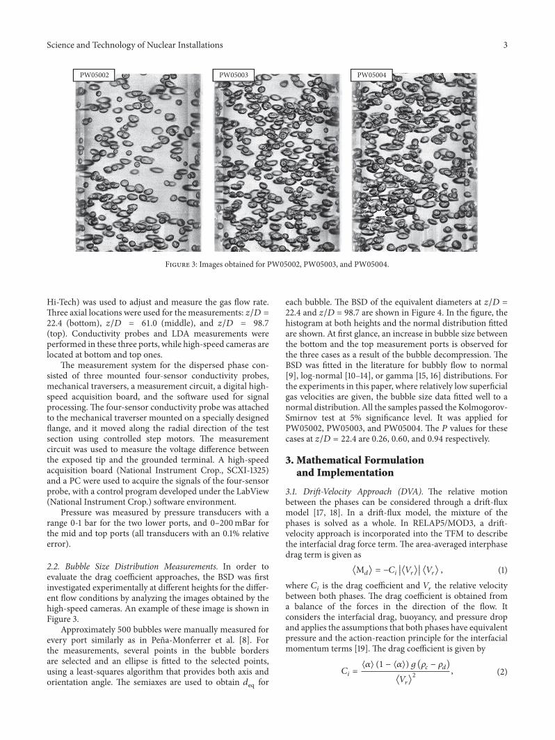
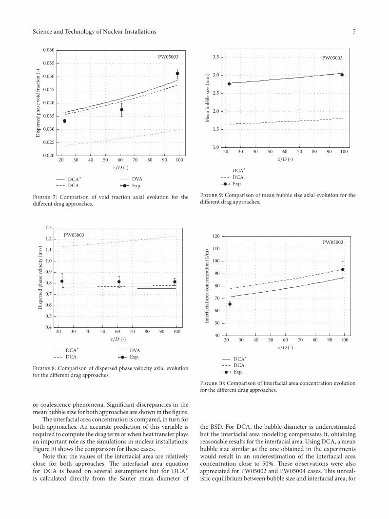
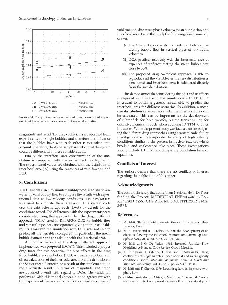

Hindawiwwwhindawicom Volume 2018
Nuclear InstallationsScience and Technology of
TribologyAdvances in
Hindawiwwwhindawicom Volume 2018
International Journal of
AerospaceEngineeringHindawiwwwhindawicom Volume 2018
OpticsInternational Journal of
Hindawiwwwhindawicom Volume 2018
Antennas andPropagation
International Journal of
Hindawiwwwhindawicom Volume 2018
Power ElectronicsHindawiwwwhindawicom Volume 2018
Advances in
CombustionJournal of
Hindawiwwwhindawicom Volume 2018
Journal of
Hindawiwwwhindawicom Volume 2018
Renewable Energy
Acoustics and VibrationAdvances in
Hindawiwwwhindawicom Volume 2018
EnergyJournal of
Hindawiwwwhindawicom Volume 2018
Hindawiwwwhindawicom
Journal ofEngineeringVolume 2018
Hindawiwwwhindawicom Volume 2018
International Journal ofInternational Journal ofPhotoenergy
Hindawiwwwhindawicom Volume 2018
Solar EnergyJournal of
Hindawiwwwhindawicom Volume 2018
Shock and Vibration
Hindawiwwwhindawicom Volume 2018
Advances in Condensed Matter Physics
International Journal of
RotatingMachinery
Hindawiwwwhindawicom Volume 2018
Hindawiwwwhindawicom Volume 2018
High Energy PhysicsAdvances in
Hindawiwwwhindawicom Volume 2018
Active and Passive Electronic Components
Hindawi Publishing Corporation httpwwwhindawicom Volume 2013Hindawiwwwhindawicom
The Scientific World Journal
Volume 2018
Submit your manuscripts atwwwhindawicom