On the Numerical Accuracy of Spreadsheets

JSS Journal of Statistical SoftwareApril 2010, Volume 34, Issue 4. http://www.jstatsoft.org/

On the Numerical Accuracy of Spreadsheets

Marcelo G. AlmironUniversidade Federal

de Alagoas

Bruno LopesUniversidade Federal

de Alagoas

Alyson L. C. OliveiraUniversidade Federal

de Alagoas

Antonio C. MedeirosUniversidade Federal

de Alagoas

Alejandro C. FreryUniversidade Federal

de Alagoas

Abstract

This paper discusses the numerical precision of five spreadsheets (Calc, Excel, Gnu-meric, NeoOffice and Oleo) running on two hardware platforms (i386 and amd64) andon three operating systems (Windows Vista, Ubuntu Intrepid and Mac OS Leopard).The methodology consists of checking the number of correct significant digits returnedby each spreadsheet when computing the sample mean, standard deviation, first-orderautocorrelation, F statistic in ANOVA tests, linear and nonlinear regression and distribu-tion functions. A discussion about the algorithms for pseudorandom number generationprovided by these platforms is also conducted. We conclude that there is no safe choiceamong the spreadsheets here assessed: they all fail in nonlinear regression and they arenot suited for Monte Carlo experiments.

Keywords: numerical accuracy, spreadsheet software, statistical computation, OpenOffice.orgCalc, Microsoft Excel, Gnumeric, NeoOffice, GNU Oleo.

1. Numerical accuracy and spreadsheets

Spreadsheets are widely used as statistical software platforms, and the results they providefrequently support strategical information. Spreadsheets intuitive visual interfaces are pre-ferred by many users and, despite their weak numeric behavior and programming support(Segaran and Hammerbacher 2009, p. 282), as said by B. D. Ripley in the 2002 Conferenceof the Royal Statistical Society opening lecture “Statistical Methods Need Software: A Viewof Statistical Computing”):

http://www.jstatsoft.org/

2 On the Numerical Accuracy of Spreadsheets

Let’s not kid ourselves: the most widely used piece of software for statistics isExcel.

Additionally, the European Spreadsheet Risks Interest Group (http://www.eusprig.org/)relates that many corporations use spreadsheets to account big financial transactions. If theaccuracy is poor, uncontrolled errors are likely to cost huge amounts of money. It is, therefore,of paramount importance to assess the accuracy of this kind of software artifacts in order toavoid disasters (Croll 2009; Powell et al. 2009).

Spreadsheets are widely employed by the scientific community in many applications, beinga few recent examples the works by Aliane (2008), who uses Excel for building interfacesthat ease the analysis of simulation charts for control systems, by Backman (2008), whoshows how to use Excel in linear programming, by Bianchi et al. (2008), who use Excelfor calculating the optimal treatment in a radiobiological evaluation, by Dzik et al. (2008),who propose a statistical process control using spreadsheets for training hospital employees,by Zoethout et al. (2008) who present a methodology for calculating alcohol effects or drug-alcohol interactions using spreadsheets and, among many others, by Roth (2008) who employsspreadsheets for the design of critical treatments, more specifically, dose control of high-voltage radiotherapy. With easy-to-use, intuitive interfaces and abstaining the user frommathematical formulas by function selection, they have won the preference of many users.

The scientific community seems to ignore, nevertheless, the vast literature that reports numer-ical problems that might preclude the use of spreadsheets in serious research (see, for instance,Apigian and Gambill 2004; Knusel 1998, 2005; Kruck 2006; Lindstrom and Asvavijnijkulchai1998; McCullough 2000, 2004; McCullough and Heiser 2008; McCullough and Wilson 1999,2002, 2005; Nash 2006).

One should expect that after a critical assessment is made about a spreadsheet, future versionsshould be free of mistakes. But, as pointed by Heiser (2006); McCullough (2004); McCulloughand Heiser (2008); Yalta (2008) this is often not the case.

In this article we used the methodology developed by McCullough (1998, 1999) and appliedby Altman (2002); Bustos and Frery (2006); Keeling and Pavur (2007); McCullough (2000);Vinod (2000); Yalta (2007); Yalta and Yalta (2007) for the assessment of spreadsheets in anotebook with an i386 CPU (32 bits) and a desktop iMac with an amd64 CPU (64 bits).Regarding the operating systems, we used GNU/Linux Ubuntu Intrepid kernel 2.6.27-14-generic and Microsoft Windows Vista SP1 on the i386 CPU, and Mac OS X Leopard on theamd64 CPU.

We present the analysis of five spreadsheets running in up to three operational systems:Microsoft Excel 2007 for Windows and 2008 for Mac OS (Microsoft Corporation 2007), Gnu-meric 1.8.3 for Ubuntu and 1.9.1 for Windows (The Gnumeric Team 2007), NeoOffice 2.2.5Patch 7 and 3.0 Patch 1 for Mac OS (Planamesa, Inc. 2009), GNU Oleo 1.99.16 for Ubuntu(Free Software Foundation 2000) and OpenOffice.org Calc 2.4.1 for Ubuntu and Windows,and version 3.0.1 for all three operational systems (Sun Microsystems Inc. 2009). Table 1shows a summary of the platforms and versions here assessed. These are the latest stable pre-compiled versions available for each platform at the time the experience was conducted, withthe exception of the development release of Gnumeric for Windows, which was the only buildavailable of that spreadsheet for such platform. This diversity is due to different hardwares,operating systems, versions and implementations may produce different numerical precisionresults. In fact, we observe such behavior in Section 4, and in Section 5 we conclude that

http://www.eusprig.org/

Journal of Statistical Software 3

Platform Calc Excel Gnumeric NeoOffice Oleo

Hardware OS 2.4.1 3.0.1 2007 2008 1.8.3 1.9.1 2.2.5 3.0 1.99.16

Windows X X X Xi386

Ubuntu X X X Xamd64 Mac OS X X X X

Table 1: Platforms and versions.

certain spreadsheets versions running in specific operating systems are advisable for particularoperations.

The analysis is performed checking the number of correct significant digits returned by eachspreadsheet when computing the sample mean, standard deviation, first-order autocorrelation,F statistic in one-way ANOVA tests, linear and nonlinear regression, and various distributionfunctions. The quality of the algorithms implemented for computing pseudorandom numbersis also discussed.

The rest of the paper unfolds as follows. Section 2 presents the historical background ofthese spreadsheets. Section 3 discusses the methodology for assessing the accuracy of thespreadsheets under consideration. Sections 4 and 5 present the results, discussions and linesfor future research.

2. Historical background

Beginning with the suit StarOffice, the OpenOffice.org Calc spreadsheet was released in 1999.Its source code was released under the LGPL (Lesser General Public License, Free SoftwareFoundation 2007b) in 2000, gathering a community of developers around its improvement anddevelopment of new functionalities. Calc currently offers almost all of the functions availablein Excel, and many new other functions are included in each release. The add-ons mechanismincluded in the last version aims at allowing users to easily incorporate new functionalitieswithout reinstalling the main core system.

Microsoft Excel for Mac OS was introduced to the market in 1985 as an alternative for Lotus 1-2-3, the most-used spreadsheet at the time. The first Windows version was issued in 1987. Thegreatest differential was the graphical interface which, allegedly, made its use easy by providingan intuitive access to its functionalities. Version 5.0 was introduced in 1993, supporting VisualBasic for Applications for the creation of macros to automate procedures (Ozkaya 1996). Since2007 it uses a new file type structure by default: the OOXML (Office Open XML), a Microsoftcopyrighted format which is not fully compatible with other spreadsheets. The latest version,available only for Mac OS, is the 2008 and the 2007 for Windows. It also incorporates amechanism for add-ons, but incompatible with OpenOffice.org.

Gnumeric 0.3 was released in 1998 by the GNU Project. It was intended to be a free (underGPL, General Public License, Free Software Foundation 2007a) alternative to commercialspreadsheets. Its original focus is on accuracy rather than on other facilities.

Since 2003 and now as the leading open source office suit for Mac OS, NeoOffice started as anX11-independent implementation. It was released using source code from the OpenOffice.org


suit, and it can be easily installed under the Acqua windows system. It claims that its currentversion provides all the features included in OpenOffice.org Calc, with improved speed andother functionalities (almost all related to interface and media support) common to Mac OSapplications. Such improved speed may have impact on the numerical properties of the suite.It supports many of the add-ons provided by OpenOffice.org.

Oleo used to be the main GNU spreadsheet. It can be used both with a graphical interface orin character mode. The first operational interface for the X Windows System was released in1994. Many of its functions are loaded from the GNU Scientific Library (GSL, Galassi et al.2003), a powerful numerical engine, but none of the functions herein assessed belongs to GSL.Oleo project has no maintainer currently, and no references about its numerical propertieswere found in the literature.

3. Accuracy measurement

There are three kinds of errors that may appear in numerical computation: cancellation,accumulation, and truncation errors (Kennedy and Gentle 1980). These errors are due to thefinite nature of binary computer representation of numbers (Knuth 1998, Chapter 4), and tonegligent implementation of functions.

Since the particular type (or types) of errors into which an algorithm may incur depends onmany factors (implementation, dataset, hardware and operational system, to name a few),extremely careful software development is always required.

In the following we will review the methodology employed for assessing accuracy of simplestatistical functions, provided one does not have access to the algorithms they employ. Insuch situation, the evaluation must rely on the results those functions provide when used inspecial datasets.

Because of the lack of implementation details from some vendors (e.g., Microsoft) and the hardtask required for analyzing source code, as previously said, we adopted the user evaluationviewpoint for assessing the reliability of spreadsheets. That is, we used each spreadsheet tocalculate functions for different datasets, from which we know the exact (certified) answers.Comparing these answers with the values obtained from each spreadsheet we have a measureof accuracy: the number of correct significant digits.

3.1. Base-10 logarithm and correct significant digits

One of the most convenient measures for comparing two numbers consists in computing theabsolute value of the relative error, and taking its base-10 logarithm:

LRE(x, c) =

{− log10

|x−c||c| if c 6= 0,

− log10 |x| otherwise,(1)

where x is the value computed by the software under assessment and c is the certified value.LRE (Log-Relative Error) relates to the number of significant digits that were correctlycomputed. For instance, considering x1 = 0.01521 and c1 = 0.01522, then LRE (x1, c1) =3.182415. Moreover, if x2 = 0.0000001521 and c2 = 0.0000001522, then LRE (x2, c2) =3.182415. In both cases we say that “the number of correct significant digits is approxi-mately 3”.


In the following we adopt the convention of reporting one decimal place whenever LRE (x, c) ≥1, zero if 0 ≤ LRE(x, c) < 1 and “–” otherwise; there is no worse situation than “–”.

3.2. Datasets and certified values

The Statistical Reference Datasets from the (American) National Institute of Standards andTechnology (1999), NIST for short, were utilized as benchmarks. We used four kinds ofdatasets to assess the reliability of univariate summary statistics, analysis of variance, linearand nonlinear regression. They consist of nine, eleven, eleven, and twenty-seven datasetsrespectively, classified in three levels of difficulty: low, average and high.

For univariate summary statistics, analysis of variance, and linear regression, each datasethas certified values calculated using multiple precision arithmetic to obtain 500 digits answersthat were rounded to fifteen significant digits. The same procedure was applied for nonlinearregression to achieve eleven significant digits.

NIST provides both observed (real world) and constructed data. For univariate summarystatistics, low difficulty data are Lew, Lottery, Mavro, Michelso, NumAcc1 and PiDigits; thefirst four being observed, and the last two constructed. NumAcc2 and NumAcc3 are average dif-ficulty data and NumAcc4 is the only high difficulty dataset for univariate summary statistics;they are all constructed.

NIST offers nine datasets for assessing the precision of ANOVA statistics, based on the pro-posal by Simon and Lesage (1989): SmLs01, SmLs02 and SmLs03 with low difficulty; SmLs04,SmLs05 and SmLs06 with average difficulty; and SmLs07, SmLs08 and SmLs09 with high diffi-culty. Two observed datasets are also provided: the low difficulty SiRstv, and the averagedifficulty AtmWtAg.

For linear regression, NIST gives Norris and Pontius observed datasets with low diffi-culty, NoInt1 and NoInt2 generated datatasets with average difficulty, and Filip, Longley,Wampler1, Wampler2, Wampler3, Wampler4 and Wampler5 datasets with high difficulty, beingthe first two observed and the last five generated. The models associated to these datasetsare: three linear, one quadratic, one multilinear, and six polynomial.

There is a diversity of nonlinear regression datasets supplied by NIST. Eight have low dif-ficulty: Misra1a, Chwirut2, Chwirut1, DanWood, Misra1b, Lanczos3, Gauss1 and Gauss2,being the first five observed and the remaining generated. Average difficulty data are Kirby2,Hahn1, Nelson, Misra1c, Misra1d, Roszman1, ENSO, MGH17, Lanczos1, Lanczos2 and Gauss3,where the first seven are observed and the other generated. Finally, high difficulty dataare MGH09, MGH10, Thurber, BoxBOD, Rat42, Eckerle4, Rat43 and Bennett5; the first twogenerated and the rest observed. There are four rational, sixteen exponential, and sevenmiscellaneous models for these data.

Regarding the distribution functions, those results obtained with Mathematica 5.2 by Yalta(2008) where used. These values are certified to be accurate to six significant digits for allthe distribution functions here assessed.

4. Results

Both the spreadsheet version and the hardware/software platform where it is used are factorsthat potentially may have some degree of influence. At the moment of this assessment,


Datasets Calc Excel Gnumeric NeoOffice Oleo

Lew (l) 15.0 15.0 15.0 15.0 15.0Lottery (l) 15.0 15.0 15.0 15.0 15.0Mavro (l) 15.0 15.0 15.0 15.0 15.0Michelso (l) 15.0 15.0 15.0 15.0 15.0NumAcc1 (l) 15.0 15.0 15.0 15.0 6.6PiDigits (l) 15.0 15.0 15.0 15.0 15.0NumAcc2 (a) 14.0 14.0 15.0 14.0 13.9NumAcc3 (a) 15.0 15.0 15.0 15.0 6.6NumAcc4 (h) 13.9 13.9 15.0 13.9 7.6

Table 2: LRE s for the sample mean.

the latest stable version of each spreadsheet for the latest stable version of each operatingsystem was used, namely, Excel 2007, Gnumeric 1.9.1, and Calc 2.4.1/3.0.1 were run onMicrosoft Windows Vista; Gnumeric 1.8.3, Calc 2.4.1/3.0.1 and Oleo 1.99.16 on GNU/LinuxUbuntu Intrepid; and Microsoft Excel 2008, NeoOffice 2.2.5/3.0 and Calc 3.0.1 on Mac OS XLeopard 10.5.6 (see Table 1).

The LRE values, see Equation 1, were computed using R 2.8.0 (R Development Core Team2009) on GNU/Linux Ubuntu Intrepid (kernel 2.6.27-14-generic) whose excellent numericalaccuracy has been assessed by Almiron et al. (2009).

Another important issue is the model representation in linear and nonlinear regressions. Inprevious works, the operator precedence interpretation led to wrong assessments (see Berger2007), for instance Excel computes -1^2 as 1, while R computes the same operation as -1.We used full parenthesis in all models to avoid such problem.

This section presents seventeen tables and a discussion, the later devoted to pseudorandomnumber generators (Section 4.5). The tables discuss results obtained when computing uni-variate statistics, namely, the sample mean (Table 2), the sample standard deviation (Table 3)and the sample first-lag autocorrelation (Table 4), analysis of variance (ANOVA, Table 5),linear (Table 6) and nonlinear (Tables 7, 8, 9 and 10) regressions and distribution functions(Tables 12, 13, 14, 15, 16, 17, 18 and 19). Each table presents LRE s, whenever the procedureis natively available in each spreadsheet/version/platform. In those cases where the resultsof at least two versions coincide, they are presented only once.

4.1. Univariate summary statistics

All spreadsheets offer specific functions to calculate the sample mean and standard deviation.In Calc, Excel, Gnumeric and NeoOffice, the sample mean can be computed with the AVERAGEfunction, and the standard deviation with the STDEV function. Oleo offers the functions AVG

and STD, respectively.

Table 2 shows the LRE s when computing the sample mean; the expression x = n−1∑n

i=1 xiwas used to compute the certified values. Each column presents the results of all consideredversions of each spreadsheet since they presented no differences.

We observe that Gnumeric presents the best results among all platforms, achieving the highest


Datasets Calc Excel 2007 Excel 2008 Gnumeric NeoOffice Oleo

Lew (l) 15.0 15.0 15.0 15.0 15.0 15.0Lottery (l) 15.0 15.0 15.0 15.0 15.0 15.0Mavro (l) 12.9 12.9 9.4 12.9 12.9 8.8Michelso (l) 13.8 13.8 8.2 13.8 13.8 8.2NumAcc1 (l) 15.0 15.0 15.0 15.0 15.0 –PiDigits (l) 15.0 15.0 15.0 15.0 15.0 15.0NumAcc2 (a) 15.0 11.5 11.5 15.0 15.0 12.5NumAcc3 (a) 9.4 9.4 1.4 9.4 9.4 –NumAcc4 (h) 8.2 8.2 0 8.2 8.2 –

Table 3: LRE s for the sample standard deviation.

possible precision in every situation. Calc, Excel and NeoOffice, interestingly, attained thesame precision with every but two datasets, NumAcc2 and NumAcc4, which pose average andhigh difficulty, respectively. Oleo presented the worst results, with problems mainly in datasetswith average and high difficulty.

Table 3 presents the results of assessing the precision when computing the standard deviation,whose certified values were computed with the expression

s =

√∑ni=1(xi − x)2

n− 1.

Calc, Gnumeric and NeoOffice exhibited similar behavior, achieving the same results for alldatasets, with bad results for NumAcc3 and NumAcc4. Excel 2007 presented similar resultsto Calc, Gnumeric and NeoOffice, except for the dataset NumAcc2, for which it was worse.Excel 2008 has several problems with four datasets, two of them of low difficulty. Again, theworst results were produced by Oleo.

Excel 2007 results for sample mean and standard deviation match with those calculatedin McCullough and Wilson (2005) and confirmed by McCullough and Heiser (2008).

The first-order autocorrelation certified values were calculated using the expression

r1 =

∑ni=2(xi − x)(xi−1 − x)∑n

i=1(xi − x)2.

No spreadsheet provides a specific function for computing this quantity, and it is not possi-ble to calculate it as a simple correlation using the CORREL function. Consider the samplea1, a2, . . . , an−1, an; the first-lag autocorrelation can be computed dividing the sample covari-ance between a1, . . . , an−1 and a2, . . . , an, divided by the sample variance of a1, a2, . . . , an−1, an.All spreadsheets provide the functions COVAR and VAR. Oleo does not provide any native func-tion for computing the first-order autocorrelation or the covariance, and, therefore, was notassessed with respect to this quantity.

Table 4 concludes the analysis of univariate summary statistics with the results for the first-order autocorrelation coefficient. With the exception of NumAcc1, samples of low level of com-plexity are the ones that produce the worst results consistently across spreadsheets, versions


Calc Excel NeoOfficeDatasets †/‡ 2007/2008 Gnumeric 2.2.5/3.0

Lew (l) 5.0 5.0 5.0 5.0Lottery (l) 3.5 3.5 3.5 3.5Mavro (l) 4.1 4.1 4.1 4.1Michelso (l) 5.9 5.9/5.8 5.9 5.9NumAcc1 (l) 15.0 15.0 15.0 15.0PiDigits (l) 5.3 5.3 5.3 5.3NumAcc2 (a) 14.4/15.0 11.3 15.0 11.5/15.0NumAcc3 (a) 12.3 12.3/0.9 12.2 –/12.2NumAcc4 (h) 11.0 11.0/NA 11.0 –/11.0

Table 4: LRE s for the sample autocorrelation coefficient († Ubuntu versions, ‡ Mac OS andWindows versions).

and platforms. The smallest values of LRE are produced by Excel 2008 and NeoOffice 2.2.5and, in particular, these spreadsheets did not return any correct digit for NumAcc3 andNumAcc4.

The computation of the first-lag autocorrelation reveals differences among versions. RegardingExcel, it loses more than ten correct digits when switching from version 2007 to 2008 andusing NumAcc3 e NumAcc4.NeoOffice also presents differences of the same order in these samedatasets, but the newer version is improved with respect to the older one.

Finally, Calc exhibits a small difference with respect to operating systems when computingthe first-lag autocorrelation of NumAcc2: its Mac OS and Windows versions produce resultsof almost one more correct digit with respect to Ubuntu.

4.2. Analysis of variance

Only Excel 2007 and Gnumeric provide native functions for computing ANOVA, so the ac-curacy of its F statistic was only assessed for these two spreadsheets. We used Analysis

ToolPak in Excel, and ANOVA in Gnumeric. Table 5 shows that both platforms achievedgood results when low and average difficulty datasets are examined. We also observe thatwhen they return different results, Gnumeric is better than Excel 2007. It is noteworthy thatExcel 2007 produced an unacceptable result for the SmLs09 dataset.

As for sample mean and standard deviation, Excel 2007 results for F statistic in ANOVA arein agreement with those reported by McCullough and Wilson (2005) and confirmed by Mc-Cullough and Heiser (2008).

4.3. Linear regression

Calc, Excel, Gnumeric and NeoOffice provide the LINEST function for linear regression inevery version/platform here assessed. Table 6 presents the LRE values of the least accuratecoefficient β and residual standard deviation (RSD) provided by each platform.

In the following tables, “NA” denotes situations for which no numeric answer is returned by


Datasets Excel 2007 Gnumeric

SiRstv (l) 13.0 13.0SmLs01 (l) 15.0 15.0SmLs02 (l) 13.8 15.0SmLs03 (l) 13.0 15.0AtmWtAg (a) 10.1 10.1SmLs04 (a) 10.4 10.4SmLs05 (a) 10.2 10.2SmLs06 (a) 10.1 10.1SmLs07 (h) 4.1 4.4SmLs08 (h) 1.8 4.1SmLs09 (h) – 4.1

Table 5: LRE s for ANOVA F statistic.

Calc‡ Excel GnumericCalc† NeoOffice 2007/2008 1.8.3/1.9.1

Datasets β RSD β RSD β RSD β RSD

Norris (l) 12.3 11.7 12.8 10.7 12.0 14.0 12.7 13.8/13.9Pontius (l) 11.5 9.3 11.2 8.9 12.0 12.7 11.0 13.0/13.4NoInt1 (a) 15.0 – 15.0 – 15.0 15.0 14.7 15.0NoInt2 (a) 15.0 – 15.0 – 15.0 14.6 15.0 15.0/14.9Filip (h) – NA – NA 7.2/6.4 7.2/6.4 0 0Longley (h) 8.6 10.1 8.5 8.7 13.3 14.4 NA NAWampler1 (h) 7.0 1.6 7.3 1.4 9.9 10.4 9.3 8.9Wampler2 (h) 9.4 6.6 10.1 6.3 13.4 15.0 10.5 12.7Wampler3 (h) 7.0 10.2 7.3 9.9 10.0 11.4 9.3 11.7Wampler4 (h) 7.0 11.8 7.3 11.1 8.1 11.8 9.3 11.7Wampler5 (h) 7.0 11.8 7.3 11.1 6.1 12.0 9.3 11.7

Table 6: LRE s for the least accurate coefficient β and residual standard deviation (RSD).† versions 2.4.1 and 3.0.1 for Ubuntu; ‡ Calc 3.0.1 for Windows and Mac OS, and also Calc 2.4.1for Windows.

the spreadsheet; a “#NUM!” is placed in the cell where the result is expected, probably due tothe fact that huge values are involved.

As Table 6 presents, regarding β, Excel 2007 provides the best or equally good results inseven out of eleven datasets, and it is the only spreadsheet that provides (low-quality, withapproximately only seven correct digits) results for the Filip dataset. Excel 2008 matchesExcel 2007’s performance in all but one situation, namely for the Filip dataset, where theformer misses about one digit with respect to the latter. Excel is outperformed by Calc 3.0.1(Windows and Mac OS), Calc 2.4.1 (Windows) and NeoOffice when dealing with the lowdifficulty Norris dataset. Gnumeric is the best spreadsheet with two datasets that offer high


difficulty, namely Wampler4 and Wampler5.

Regarding the RSD, as Table 6 presents, Excel 2007 produces the most accurate results (oras good results as other spreadsheets) in eight out of eleven situations. Excel 2008 matchesExcel 2007’s performance in all but the Filip dataset where, again, the former misses aboutone digit with respect to the latter. In the three situations where Excel is not the bestplatform, it is outperformed by Gnumeric; it happens with datasets having low, average andhigh difficulty.

McCullough (1998) suggests that at least nine correct digits should be expected in low-difficulty linear regression procedures.

As observed for sample mean, standard deviation and F statistic in ANOVA, Excel 2007results for linear regressions match with those observed for McCullough and Wilson (2005)and confirmed by McCullough and Heiser (2008).

4.4. Nonlinear regression

Nonlinear regression was assessed with a suite of 27 datasets, transforming each regressioninto a nonlinear optimization problem, where the objective is minimizing the residual sum ofsquares. To achieve this, we used the general tool Solver.

The only spreadsheets that provide natively Solver with such capability are Calc 2.4.1 forUbuntu, Excel 2007 and NeoOffice 2.2.5. The Solver from Excel 2007 provides two methodsfor solving nonlinear regression problems, namely Newton and Conjugate; they were bothassessed.

By default, Calc 3.0.1 and NeoOffice 3.0 only provide a Solver for linear regression. Anextension named Solver for Nonlinear Regression enabled the analysis on these spread-sheets. This extension can be found in the official site for extensions of OpenOffice.org(http://extensions.services.openoffice.org/), in a package provided by Sun Microsys-tems Inc. (who is also the holder of OpenOffice.org Calc copyright) under the LGPL license(for more information about this extension see http://wiki.services.openoffice.org/

wiki/NLPSolver). This extension provides two non-deterministic evolutionary algorithms:DEPS and SCO.

DEPS (differential evolution particle swarm) is a hybrid multiagent approach based on theparticle swarm optimization paradigm (Zhang and Xie 2003), while SCO (social cognitiveoptimization) is based on social intelligence and human learning mechanisms (Xie et al. 2002).

Most algorithms considered here accept adjustments, despite loading with default parameters.Nevertheless, as McCullough (1998) comments, adjusting these settings may result in bettersolutions. In the following we assess these techniques with both the default parameters andsets chosen to improve results.

Nonlinear optimization procedures usually require starting points, and Solver is no exception.Each dataset is provided by NIST with two starting points: the first (denoted ‘Start 1’ inTables 7 and 9) is far from final solution and it represents the usual situation where the userhas no prior idea as to where the solution is. The second (denoted ‘Start 2’ in Tables 8 and 10)is closer to final solution.

Using default settings

This situation describes the user who has no prior idea about both the problem, its solution

http://extensions.services.openoffice.org/

http://wiki.services.openoffice.org/wiki/NLPSolver

http://wiki.services.openoffice.org/wiki/NLPSolver


●

● ●

●

●

●

2 4 6 8 10

120

140

160

180

200

220

x

y

CertifiedCalc 2.4.1 (U) andNeoOffice 2.2.5Conjugate and Newton

(a) BoxBOD dataset from Start 2 in Calc 2.4.1 forUbuntu, NeoOffice 2.2.5 and Excel 2007

●●●●●●●●● ● ●●

●●

●

●

●●

●

●

●●

●

●

●●●

●●

● ●●●

● ●● ●

−3 −2 −1 0 1 2

200

400

600

800

1000

1200

1400

x

y

CertifiedConjugateNewton

(b) Thurber dataset from start 2 in Excel 2007

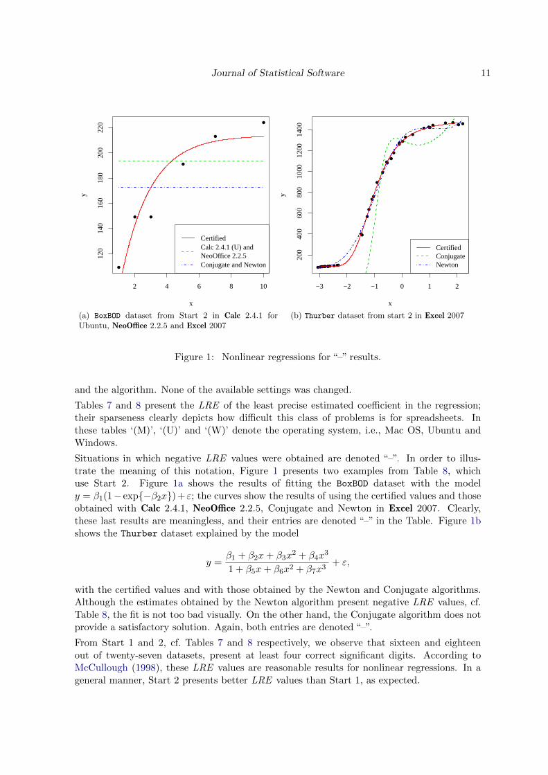
Figure 1: Nonlinear regressions for “–” results.

and the algorithm. None of the available settings was changed.

Tables 7 and 8 present the LRE of the least precise estimated coefficient in the regression;their sparseness clearly depicts how difficult this class of problems is for spreadsheets. Inthese tables ‘(M)’, ‘(U)’ and ‘(W)’ denote the operating system, i.e., Mac OS, Ubuntu andWindows.

Situations in which negative LRE values were obtained are denoted “–”. In order to illus-trate the meaning of this notation, Figure 1 presents two examples from Table 8, whichuse Start 2. Figure 1a shows the results of fitting the BoxBOD dataset with the modely = β1(1− exp{−β2x}) + ε; the curves show the results of using the certified values and thoseobtained with Calc 2.4.1, NeoOffice 2.2.5, Conjugate and Newton in Excel 2007. Clearly,these last results are meaningless, and their entries are denoted “–” in the Table. Figure 1bshows the Thurber dataset explained by the model

y =β1 + β2x+ β3x

2 + β4x3

1 + β5x+ β6x2 + β7x3+ ε,

with the certified values and with those obtained by the Newton and Conjugate algorithms.Although the estimates obtained by the Newton algorithm present negative LRE values, cf.Table 8, the fit is not too bad visually. On the other hand, the Conjugate algorithm does notprovide a satisfactory solution. Again, both entries are denoted “–”.

From Start 1 and 2, cf. Tables 7 and 8 respectively, we observe that sixteen and eighteenout of twenty-seven datasets, present at least four correct significant digits. According toMcCullough (1998), these LRE values are reasonable results for nonlinear regressions. In ageneral manner, Start 2 presents better LRE values than Start 1, as expected.


Datasets Cal

c2.4.1

(U)

Cal

c3.0.1

–D

EP

S(M

)

Cal

c3.

0.1

–SC

O(M

)

Cal

c3.0.1

–D

EP

S(U

)

Cal

c3.

0.1

–SC

O(U

)

Cal

c3.0.1

–D

EP

S(W

)

Cal

c3.

0.1

–SC

O(W

)

Exce

l200

7–

Conju

gate

Exce

l200

7–

New

ton

Neo

Offi

ce2.

2.5

Neo

Offi

ce3.0

–D

EP

S

Neo

Offi

ce3.

0–

SC

O

Misra1a (l) 0 0 0 0 0 0 0 – 1.6 – 0 0Chwirut2 (l) – 5.6 4.4 4.8 4.9 6.1 5.0 0 4.3 0 5.4 4.8Chwirut1 (l) – 5.1 5.1 5.1 4.8 4.9 4.5 1.7 4.0 0 5.5 4.4Lanczos3 (l) – 0 – 0 – 0 – – – – – –Gauss1 (l) 0 5.7 6.1 5.8 5.9 6.0 5.7 1.0 4.8 0 6.1 5.8Gauss2 (l) 0 5.8 – 6.1 – 5.9 5.3 1.3 4.6 0 5.9 –DanWood (l) 1.1 4.3 4.1 4.7 5.0 4.6 4.2 4.0 4.7 1.0 4.2 4.8Misra1b (l) 0 4.8 4.9 5.7 4.8 5.3 5.3 0 0 0 5.1 5.6Kirby2 (a) 0 4.6 0 4.7 0 4.4 0 0 0 0 4.7 0Hahn1 (a) – 4.1 – 3.6 – 3.0 – – – – 3.1 –Nelson (a) – – – – – – – – – – – –MGH17 (a) – – – 0 – – – – – – – –Lanczos1 (a) – 0 – – – 0 – – – – – –Lanczos2 (a) – – – – – – – – – – 0 –Gauss3 (a) 0 5.9 – 6.0 – 6.1 3.0 0 4.3 0 5.4 0Misra1c (a) – 5.4 5.3 5.5 4.9 5.3 5.2 0 2.5 – 4.8 4.9Misra1d (a) 0 6.0 4.5 5.9 4.6 4.7 5.4 0 1.0 – 5.0 4.6Roszman1 (a) – 2.2 1.2 1.5 1.3 2.1 1.2 – – 0 2.0 2.0ENSO (a) – – 3.0 – – – – 2.1 3.4 – 4.2 3.5MGH09 (h) – – – – – – – – – – – –Thurber (h) 0 5.8 0 5.8 0 6.1 0 – 1.3 0 6.6 0BoxBOD (h) – – – – – – – – – – – –Rat42 (h) – 5.6 5.7 5.6 5.2 5.2 5.9 0 5.9 – 5.7 5.8MGH10 (h) – 6.5 – 6.7 – 6.1 – – – – 6.2 –Eckerle4 (h) – 3.8 3.3 3.8 3.7 3.9 4.6 – – – 3.4 4.0Rat43 (h) – – – – – – – – – 0 – –Bennett5 (h) – 0 0 2.8 0 0 0 0 0 0 0 0

Table 7: LRE s for non-linear regression from Start 1, default parameters.

Results obtained from Start 1 can be analyzed according to the dataset complexity. Withinlow difficulty, for all but two datasets there are good results presented by at least one al-gorithm; no algorithm computes reliable values for Misra1a and Lanczos3 datasets. More-over, Chwirut2, Chwirut1, Gauss1, Gauss2 and Misra1b dataset are difficult for Conjugate(Excel 2007). Calc 2.4.1 and NeoOffice 2.2.5 presented no reliable values in any dataset. AsTable 7 shows, the best results are obtained with DEPS algorithm, regardless the spreadsheet


Datasets Cal

c2.4.1

(U)

Cal

c3.0.1

–D

EP

S(M

)

Cal

c3.

0.1

-SC

O(M

)

Cal

c3.0.1

-DE

PS

(U)

Cal

c3.

0.1

–SC

O(U

)

Cal

c3.0.1

–D

EP

S(W

)

Cal

c3.

0.1

–SC

O(W

)

Exce

l200

7–

Conju

gate

Exce

l200

7–

New

ton

Neo

Offi

ce2.

2.5

Neo

Offi

ce3.0

–D

EP

S

Neo

Offi

ce3.

0–

SC

O

Misra1a (l) 1.3 5.3 5.0 5.4 5.2 5.9 6.2 1.3 1.3 – 6.1 5.8Chwirut2 (l) 0 5.8 5.1 5.1 5.1 5.6 5.1 1.0 4.7 1.3 5.3 4.8Chwirut1 (l) – 5.7 4.7 5.4 5.6 5.1 5.0 1.0 4.9 0 5.7 4.9Lanczos3 (l) – – – – – – – – – – – –Gauss1 (l) 1.1 6.0 5.7 5.8 5.5 5.8 6.0 1.4 4.6 1.1 6.1 6.0Gauss2 (l) 0 5.9 – 5.9 0 5.7 0 0 4.5 0 5.9 0DanWood (l) 3.4 4.1 4.0 4.8 5.1 4.7 4.6 5.1 4.8 1.9 4.7 4.3Misra1b (l) 0 5.2 5.3 5.3 5.2 5.5 6.0 0 2.8 0 5.3 5.7Kirby2 (a) 0 4.6 – 4.7 – 4.0 – 0 0 0 4.5 0Hahn1 (a) 0 3.6 – 3.1 – 3.7 0 – – 0 3.7 –Nelson (a) – 2.9 2.3 3.6 2.6 3.0 2.3 0 0 0 3.2 3.5MGH17 (a) 0 1.2 0 1.3 0 1.1 0 0 0 0 1.2 0Lanczos1 (a) – – – – – – – – – – – –Lanczos2 (a) – – – – – – – – – – – –Gauss3 (a) 0 6.0 2.9 5.8 – 5.7 0 0 4.4 0 5.8 0Misra1c (a) 1.2 5.7 5.3 5.7 5.4 5.4 5.4 1.1 1.2 1.1 5.9 5.1Misra1d (a) 0 5.0 4.7 5.5 5.4 5.5 5.5 1.5 1.5 1.5 5.5 6.0Roszman1 (a) 0 1.9 0 1.7 2.2 1.7 0 0 0 0 2.5 1.2ENSO (a) – 1.2 1.2 1.2 1.2 1.2 – 2.5 3.4 – 1.2 –MGH09 (h) – 1.8 0 1.7 1.3 1.8 1.5 1.1 4.3 – 1.7 0Thurber (h) 0 6.2 1.3 5.8 1.0 5.7 0 – – 0 6.0 1.2BoxBOD (h) – 5.9 6.7 6.2 6.0 6.9 5.7 – – – 5.9 5.5Rat42 (h) – 5.9 5.0 5.4 5.1 5.7 5.6 1.2 5.2 – 5.7 5.5MGH10 (h) – 5.8 0 6.8 0 7.1 1.5 – – – 6.0 –Eckerle4 (h) 0 4.0 3.8 3.7 3.7 3.8 3.4 5.1 4.7 0 3.8 3.7Rat43 (h) – 5.7 2.3 5.2 2.0 5.3 3.9 2.1 3.5 1.3 5.2 2.3Bennett5 (h) – 0 0 0 1.2 0 0 0 0 0 0 1.1

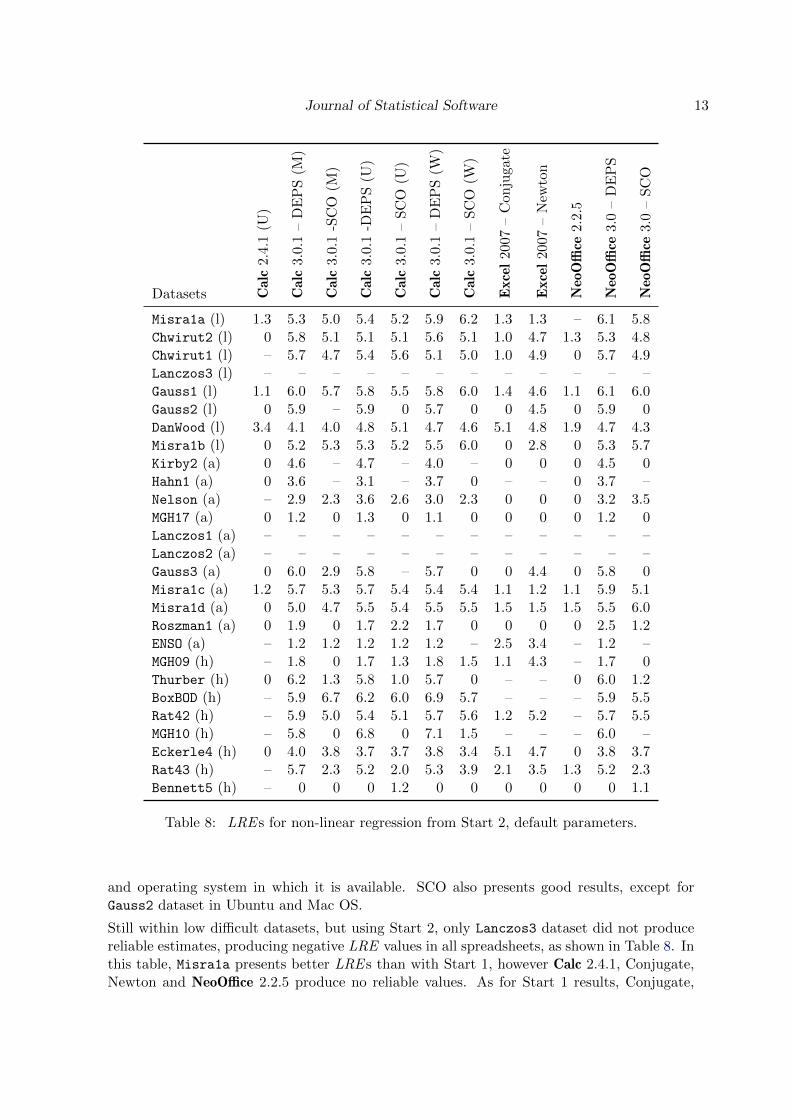
Table 8: LRE s for non-linear regression from Start 2, default parameters.

and operating system in which it is available. SCO also presents good results, except forGauss2 dataset in Ubuntu and Mac OS.

Still within low difficult datasets, but using Start 2, only Lanczos3 dataset did not producereliable estimates, producing negative LRE values in all spreadsheets, as shown in Table 8. Inthis table, Misra1a presents better LRE s than with Start 1, however Calc 2.4.1, Conjugate,Newton and NeoOffice 2.2.5 produce no reliable values. As for Start 1 results, Conjugate,


Calc 2.4.1 and NeoOffice 2.2.5 achieved the worst accuracy. Again the best results are pro-duced by the DEPS algorithm. The SCO algorithm produces no improvement when dealingwith the Gauss2 dataset. Moreover, its Windows version led to a worse result than therespective in Start 1.

Analyzing average difficult datasets, we found many problems in Start 1. Nelson, MGH17,Lanczos1, Lanczos2 and Roszman1 represent a great challenge for all algorithms herein as-sessed, and no reliable values were achieved. For the rest of datasets, DEPS achieved thebest results, even for ENSO for which DEPS is the only one to present an acceptable LRE .Calc 2.4.1, Conjugate and NeoOffice 2.2.5 could not deal with any dataset with good resultsand Newton did it only for Gauss3.

Regarding the use of Start 2, for average difficult datasets, Table 8 shows significative im-provements for Nelson, MGH17 and Roszman1, however these do not represent reliable answers.Furthermore the results for Lanczos1 and Lanczos2 are even worse than the ones obtainedfrom Start 1. Due to the nondeterministic nature of DEPS and SCO algorithms, there is notenough evidence to state that improvements were achieved using Start 2. DEPS presents,nevertheless, the best LRE values. The poor performance of Calc 2.4.1, Conjugate, Newtonand NeoOffice 2.2.5, observed from Start 1, does not improve significantly when switchingto Start 2. As DEPS, SCO algorithm presents reliable results for some datasets, but it failsestimating parameters correctly for Kirby2, Hahn1, and Gauss3.

Focusing the analysis on highly difficult datasets, we observe from Table 7 that using Start 1leads to no correct significant digit with any algorithm for MGH09, BoxBOD and Rat43. Bennett5also represents a very difficult situation for all algorithms, and no reliable results were ob-served. Almost reasonable results for Eckerle4 can be computed only by DEPS and SCO.In the rest of datasets, the best results are obtained with DEPS and SCO, in that order.

As Table 8 shows, many improvements were obtained using Start 2. The most noticeablechange was reached for BoxBOD dataset. Here, from negative LRE values achieved fromStart 1, reliable results were computed with DEPS and SCO algorithms using Start 2. Re-garding DEPS only, this also happens for Rat43. Newton presents improvements related toMGH09 and Eckerle4 datasets.

For any dataset complexity, there are situations for which no algorithm is able to computereliable results using the default algorithm parameters. DEPS presents, nevertheless, thebest LRE values for almost all comparisons regarding nonlinear regression when using defaultsettings.

Customizing Solver settings

The blind use of default settings, though highly undesirable, is often found in practice. Forinstance, Knight (2002) and Kaiser (2002) report erroneous results obtained by pollutionresearchers in North America and Europe, when using default settings in a regression model.They report the problem as a software glitch, when, in fact, it is not. We emphasize thatthere is no safety in using the default settings when applying regressions, especially nonlinearregressions.

In the following, we present the assessment of nonlinear regressions with customized settings.Each Solver has its own parameters, according to the algorithm used, so it is not possibleto discuss a single set of parameters; parameters identified as having similar effect were setequal. Speed was not considered in the performance of the algorithms, only the numerical


accuracy.

Firstly, we consider the parameters which are common to the two nonlinear algorithms avail-able for Excel. In order to avoid, as much as possible, time or iterations limits we used 32, 767seconds for max time (upper bound available by the software) and 2, 000 as upper bound foriterations. The convergence was set to 1E − 8 and, as recommended by this Solver doc-umentation, we chose forward derivatives and tangent estimates. The rest of the parameterswere kept as default.

Secondly, we customized the DEPS and SCO algorithms. Size of swarm and stagnation

limit were set to 150. Bigger values were tested, but no LRE improvements were observed.The stagnation tolerance has an analogy with the tolerance parameter of Excel, andthen we used the same value in both cases, namely 1E − 8. Again, all other parameter werekept as default.

Calc 2.4.1 and NeoOffice 2.2.5 do not appear in this analysis because they are not customiz-able. Following the strategy conducted with the default settings, we present in Tables 9and 10 the LRE of the least precise estimated coefficient in each regression. Once again, weused ‘(M)’, ‘(U)’ and ‘(W)’ in these tables to denote the operating system.

In a general manner, from Start 1 and 2, the algorithms with customized parametrizationyielded better results than those obtained with default settings. Tables 9 and 10 show that,from Start 1 and 2, twenty and twenty-three respectively of twenty-seven datasets satisfiedthe four correct significant digits of accuracy requested by the McCullough (1998) criterion.

As Table 9 shows, reasonable LRE values were obtained for low difficulty datasets, with theexception of Misra1a and Gauss2. We highlight that Newton is the only algorithm that dealtwith these two datasets in a satisfactory way. DEPS algorithm obtained good LRE valuesfor Gauss2 as well.

Lanczos3 is the only low difficulty dataset for which no significant digits were reached fromStart 1 by any algorithm herein assessed.

Observing results achieved for low difficulty datasets from Start 2 in Table 10, we note that webetter LRE values are obtained when compared with Start 1. Only problems with Lanczos3

dataset were observed.

A common issue from Start 1 and 2 is the poor precision obtained by the SCO algorithm.The biggest LRE values were obtained with the Newton algorithm for both starting points.DEPS is more robust than the rest of algorithms, as can be seen in Tables 9 and 10.

Regarding average difficulty datasets, we note from Table 9 that three out of eleven datasetsdo not present satisfactory LRE values in the Start 1 case: MGH17, Lanczos1 and Lanczos2

(these two last did not produce a single correct digit). Though the overall results are improvedwith respect to those obtained without parameter tuning, cf. Table 7, they are still not reliableenough; only Misra1c e Misra1d produce acceptable results, within these datasets, in eightand nine, respectively, of the situations. Best results are obtained by DEPS and Newton.

Considering Start 2 in Table 10, we still observe problems in Lanczos1 and Lanczos2 datasets.Concerning all datasets but these two, we obtained satisfactory results for six out of elevendatasets using DEPS algorithm, and six out of eleven using Newton. SCO algorithm reachedacceptable results for three of these cases, and Conjugate only for two of them.

With regard to high difficult datasets, we observe that for Start 1 we get reliable results infive out of eight datasets (see Table 9). DEPS algorithm deals correctly with four of these


Datasets Cal

c3.0.1

–D

EP

S(M

)

Cal

c3.

0.1

–SC

O(M

)

Cal

c3.0.1

–D

EP

S(U

)

Cal

c3.

0.1

–SC

O(U

)

Cal

c3.0.1

–D

EP

S(W

)

Cal

c3.

0.1

–SC

O(W

)

Exce

l200

7–

Conju

gate

Exce

l200

7–

New

ton

Neo

Offi

ce3.

0–

DE

PS

Neo

Offi

ce3.0

–SC

O

Misra1a (l) 0 0 0 0 0 0 – 4.5 0 0Chwirut2 (l) 6.3 6.3 6.4 5.6 5.8 6.0 4.6 7.0 6.8 6.2Chwirut1 (l) 6.6 6.3 6.4 6.8 6.6 7.3 4.4 7.1 6.8 6.2Lanczos3 (l) 0 – 0 – 0 – – – – –Gauss1 (l) 7.0 7.1 6.7 6.7 6.7 7.0 4.0 7.6 6.9 6.7Gauss2 (l) 7.0 – 7.0 – 6.8 – 3.6 7.5 7.2 –DanWood (l) 5.7 5.8 6.5 6.3 5.3 4.8 9.1 9.8 6.2 5.7Misra1b (l) 6.1 5.6 5.9 6.3 6.5 5.8 0 5.6 6.5 5.7Kirby2 (a) 5.2 0 5.3 0 5.3 0 0 0 5.1 0Hahn1 (a) 4.7 0 4.8 – 5.0 – – – 4.7 –Nelson (a) – – – – – – 0 4.8 – –MGH17 (a) 3.1 – – – 3.5 – – – 3.1 –Lanczos1 (a) 0 – 0 – 0 – – – 0 –Lanczos2 (a) 0 – 0 – 0 – – – 0 –Gauss3 (a) 6.8 – – – 6.5 0 2.4 7.6 6.8 –Misra1c (a) 5.9 6.0 8.0 6.0 7.0 5.9 0 2.9 5.9 6.0Misra1d (a) 7.5 6.0 6.3 7.5 6.3 6.2 0 4.0 7.5 6.1Roszman1 (a) 3.2 1.2 2.6 1.3 2.7 1.5 – 9.1 3.2 9.0ENSO (a) – – – – – – 5.8 7.3 – –MGH09 (h) – – – – – – – – – –Thurber (h) 7.0 0 7.1 0 7.0 0 – 7.4 7.0 0BoxBOD (h) – – – – – – 8.7 9.0 – –Rat42 (h) 6.2 6.7 6.2 6.2 6.5 6.1 4.8 8.4 6.2 6.0MGH10 (h) 7.1 – 7.0 – 7.3 – – – 7.1 –Eckerle4 (h) 5.0 4.8 4.9 5.1 4.7 4.9 – – 5.0 4.8Rat43 (h) – – – – – – – – – –Bennett5 (h) 0 0 0 0 1.7 0 0 0 0 –

Table 9: LRE s for customized non-linear regression from Start 1

datasets, and Newton reached satisfactory LRE values for three of them. Both SCO andConjugate algorithms have problems with all but two datasets.

Additionally, we observe big differences between Start 2 and Start 1 (see Tables 9 and 10).The only one dataset from Start 2 for which there are problems is Bennett5. The best resultsin this case were found with DEPS algorithm, which reached reasonable results for six of eightdatasets. On the other hand, Newton obtained satisfactory LRE values for five of these high


Datasets Cal

c3.0.1

–D

EP

S(M

)

Cal

c3.

0.1

–SC

O(M

)

Cal

c3.0.1

–D

EP

S(U

)

Cal

c3.

0.1

–SC

O(U

)

Cal

c3.0.1

–D

EP

S(W

)

Cal

c3.

0.1

–SC

O(W

)

Exce

l200

7–

Conju

gate

Exce

l200

7–

New

ton

Neo

Offi

ce3.

0–

DE

PS

Neo

Offi

ce3.0

–SC

O

Misra1a (l) 6.0 6.0 6.1 5.9 6.5 6.3 1.3 4.3 6.7 6.6Chwirut2 (l) 6.3 6.0 5.9 5.5 6.3 6.2 3.5 7.0 6.2 6.1Chwirut1 (l) 6.2 6.4 7.1 6.3 6.9 6.6 4.9 7.0 6.2 6.4Lanczos3 (l) – – – – – – – – – –Gauss1 (l) 7.1 6.9 7.1 7.3 7.0 7.2 4.3 7.6 6.7 6.7Gauss2 (l) 7.2 – 7.1 – 7.2 – 3.6 7.5 7.2 6.8DanWood (l) 5.6 5.2 5.7 4.9 6.0 5.3 9.0 9.4 5.3 5.7Misra1b (l) 5.9 6.2 6.9 6.6 7.0 5.8 0 3.4 6.1 6.3Kirby2 (a) 5.8 0 5.6 0 5.6 0 0 0 4.9 0Hahn1 (a) 4.4 0 4.2 – 4.7 – – – 4.4 –Nelson (a) 5.0 4.0 4.3 4.0 4.2 4.2 0 4.8 4.1 3.7MGH17 (a) 3.5 0 1.2 0 3.1 0 0 4.4 3.5 0Lanczos1 (a) – – – – – – – – – –Lanczos2 (a) – – 1.1 – – – – – – –Gauss3 (a) 6.7 3.6 6.4 0 7.0 – 2.9 7.8 6.7 –Misra1c (a) 7.0 6.3 6.0 7.3 6.2 6.2 1.2 3.1 7.0 6.5Misra1d (a) 6.4 6.6 6.5 5.8 6.7 6.6 1.5 3.3 6.4 6.6Roszman1 (a) 2.8 1.3 3.5 2.6 2.5 1.4 0 8.1 2.8 1.4ENSO (a) 1.2 – 1.2 1.2 1.2 1.2 6.2 6.5 1.2 –MGH09 (h) 2.7 2.3 2.5 2.3 2.6 2.4 3.4 5.0 2.7 2.0Thurber (h) 6.5 0 6.8 0 6.8 0 0 7.2 6.5 0BoxBOD (h) 7.4 7.4 7.1 7.1 7.3 8.0 – – 7.4 6.9Rat42 (h) 6.5 6.9 6.7 6.5 6.1 6.7 6.2 8.5 6.5 6.7MGH10 (h) 7.9 – 7.2 – 7.3 – – 1.4 7.9 –Eckerle4 (h) 4.7 4.7 – 4.7 4.9 4.8 6.2 5.9 4.7 5.1Rat43 (h) 6.4 4.2 7.1 4.3 7.1 4.6 3.7 8.9 6.4 4.9Bennett5 (h) 1.2 0 1.4 0 0 0 0 0 1.2 1.5

Table 10: LRE s for customized non-linear regression from Start 2.

difficulty datasets. We remark that the worst results were reached applying the Conjugatealgorithm.

An overview of the three kinds of datasets complexity shows that we get improved LREvalues when using Start 2. This issue lead to assert that almost all algorithm take advantageof closer initial points, as expected.


Calc Excel 2007 Excel 2008 Gnumeric NeoOffice Oleo

Documentation N Y-wrong N Y N NSeed N Y N N N N

Table 11: Documentation and seed availability of pseudorandom number generators.

Results achieved with customized settings from Start 2 are roughly the upper bound of reli-ability that we can get using spreadsheets as nonlinear solvers.

A third starting point was also used with customized parameters: the certified value. It isuseful to assess the algorithm’s ability to identify when it has reached the solution. Conjugateand Newton (available in Excel) recognized when the current solution is optimal in all butwith the Bennett5 dataset. DEPS (from Calc and NeoOffice) fails more often: 12, 13 and 9times out of 27 datasets, in Windows, Mac OS and Ubuntu, respectively. It is noteworthy,though, that even failing to stop at the certified value, DEPS provides at least LRE = 7 inall datasets but Rat43, for which negative LRE values were obtained, and Bennett5, whereone significant correct digit was computed.

4.5. Pseudorandom number generation

According to Ripley (1987, 1990) good pseudorandom number generators ought to providesequences of numbers with the following properties:

1. they resemble outcomes from uniformly-distributed random variables,

2. vectors of moderate dimensions of those random variables are collectively independent,

3. repeatability from a few easily to specify parameters, the seed, in a wide variety ofcomputational environments (hardware, operating system, programming language),

4. speed,

5. long periods.

Verifying the two first properties for a given sequence is tough, and a number of tests hasbeen proposed in the literature. Marsaglia’s Diehard tests (Marsaglia 1995) and the NISTRandom Number Generation standard (Rukhin et al. 2008) are some of the tools availablefor such assessment.

From the user viewpoint, good documentation that may lead to informed decisions wouldsuffice. Table 11 presents a summary of the documentation and setting seed availability of allthe spreadsheets under assessment.

Calc’s documentation provides no information about the algorithm implemented and providesno user function for setting the seed. The source code claims that it uses the C rand function(which has no default implementation specified in the ISO C standard – ISO/IEC 9899:TC2)in its RNG. The only information is that the function generates numbers between 0 and, atleast, 32767. Therefore according to the implementation adopted into the library (stdlib.h)used to compile it, a new RNG may be produced yielding, thus, a non-portable function.


NeoOffice, which is based on OpenOffice.org, suffers from the same issue. From the user’s per-spective, Gnumeric does not provide any high-level means for setting the seed of the randomnumber generator. The generator implemented by Gnumeric is the long-period Mersenne-Twister (Matsumoto and Nishimura 1998).

Microsoft claims that Excel 2003 and 2007 use an implementation of the Wichmann andHill (1982) algorithm, but as shown by McCullough (2008a) this is not true. The samemethodology was applied to Excel 2008, and we also concluded that whichever the algorithmimplemented, it is neither the original Wichman-Hill nor the new version (Wichmann and Hill2006). The Mac OS version does not provide any information about this implementation.

Oleo provides an undocumented function for the generation of integer values in the range0, . . . , x, with x provided by the user. The only information about this function is availablein Oleo’s source code, and states that a “linear feedback shift register” is used. Once enteredthe command, the value is updated regularly at intervals from 1 to 10 seconds, at the user’schoice. There is no high-level access to the seed.

4.6. Distribution functions

According to Knusel (1995) the answer given by a program should be correct and reliable asit is printed out. Furthermore, according to Yalta (2008), good statistical software should beable to provide six or seven accurate digits for probabilities as small as 10−100.

Yalta (2008) presents a detailed assessment of the numerical issues that different versionsof Excel, versions from 97 to 2007, exhibit in statistical distributions. The author analyzesMicrosoft’s performance on correcting errors reported in the literature, and compares itsspreadsheet with Gnumeric 1.7.11 and Calc 2.3.0. No information about assessments onNeoOffice were found in the literature, to the best of our knowledge.

In this section we present the numerical accuracy of the main statistical distributions assessedby Yalta (2008), but restricted to those situations where difficulties were observed. With thisapproach we put in evidence the differences between the spreadsheets herein assessed.

The specific name and parameters of functions are the same in all platforms and versions.Gnumeric provides another sets of functions based on the R platform (Almiron et al. 2009).We tested both sets, and no differences were observed in their numerical precision. Oleo wasnot assessed since it does not provide native resources for computing distribution functions.

The function BINOMDIST(k, n, p, cum = 1) computes the probability P{X ≤ k}, where Xfollows a binomial distribution with n trials and p the probability of success on each trial.In Gnumeric, the R-based function R.PBINOM(k, n, p) can be used for the same purpose.Table 12 shows that, for n = 1030 and p = 0.5, Excel 2007 cannot compute any digitcorrectly for k ∈ {1, 2, 100, 300}, whereas Calc, Excel 2008, NeoOffice and Gnumeric, providegood accuracy in all tested cases, including those in which probabilities are much smaller than10−100.

POISSON(k, lambda, cum) computes P{X ≤ k} if cum = 1, and P{X = k} if cum = 0,where X follows a Poisson distribution with mean λ > 0. Gnumeric’s R-based functionsR.PPOIS(k, lambda) and R.DPOIS(k, lambda), for cum = 1 and cum = 0, respectively,can be used as well. For Poisson probabilities, we observe in Table 13 that, again, Excelpresents the worst results, while Calc, Gnumeric and NeoOffice, offer excellent accuracy.When computing the cumulative distribution function, Excel is unable to compute any digit


CalcExcel 2008Gnumeric

k Certified P{X ≤ k} NeoOffice Excel 2007

1 8.96114E − 308 6.0 02 4.61499E − 305 6.0 0

100 1.39413E − 169 5.5 0300 2.91621E − 42 6.0 0400 3.89735E − 13 6.0 2.1410 3.19438E − 11 5.8 4.0

Table 12: LRE s for the binomial distribution with n = 1030 and p = 0.5.

Calck λ Certified P{X = k} NeoOffice Excel Gnumeric

0 200 1.38390E − 87 5.6 0 5.6103 200 1.41720E − 14 6.0 0 6.0315 200 1.41948E − 14 6.0 0 6.0400 200 5.58069E − 36 6.0 0 6.0900 200 1.73230E − 286 6.0 0 6.0

Calck λ Certified P{X ≤ k} NeoOffice Excel Gnumeric

1E + 05 1E + 05 0.500841 NA 0 6.01E + 07 1E + 07 0.500084 NA 0 6.01E + 09 1E + 09 0.500008 NA 0 6.0

Table 13: LRE s for the Poisson distribution.

correctly, while Calc and NeoOffice do not return any numeric answer avoiding, thus, tomislead the users. Exact results can be computed with Gnumeric.

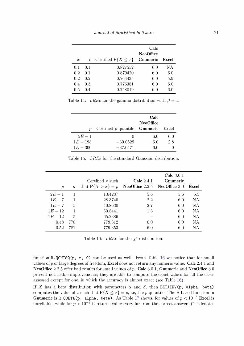
The function GAMMADIST(x, alpha, beta, cum) computes P{X ≤ x} if cum = 1, and thedensity at x if cum = 0, with X following a gamma distribution with shape α and scale β. Al-ternatively, Gnumeric’s R-based functions are R.PGAMMA(x, alpha, beta) and R.DGAMMA(x,

alpha, beta), for cum = 1 and cum = 0, respectively. As Table 14 shows, Calc, NeoOfficeand Gnumeric present exact answers for all cases of cumulative distribution functions. Excelalso presents good results except for x = 0.1, where no numerical answer is provided.

If X follows a standard Gaussian distribution, then NORMSINV(p) computes the value of x suchthat P{X ≤ x} = p, i.e., the p-quantile. Gnumeric offers the alternative R-based functionR.QNORM(p, 0, 1). Table 15 shows that Excel has serious problems for values of p < 10−198,whereas Calc, NeoOffice and Gnumeric return exact answers whenever p ≥ 10−300.

If X obeys a χ2 distribution with n degrees of freedom, then the function CHIINV(p, n)

computes the value of x such that P{X > x} = p. Alternatively, the Gnumeric’s R-based


CalcNeoOffice

x α Certified P{X ≤ x} Gnumeric Excel

0.1 0.1 0.827552 6.0 NA0.2 0.1 0.879420 6.0 6.00.2 0.2 0.764435 6.0 5.90.4 0.3 0.776381 6.0 6.00.5 0.4 0.748019 6.0 6.0

Table 14: LRE s for the gamma distribution with β = 1.

CalcNeoOffice

p Certified p-quantile Gnumeric Excel

5E − 1 0 6.0 6.01E − 198 −30.0529 6.0 2.81E − 300 −37.0471 6.0 0

Table 15: LRE s for the standard Gaussian distribution.

Calc 3.0.1Certified x such Calc 2.4.1 Gnumeric

p n that P{X > x} = p NeoOffice 2.2.5 NeoOffice 3.0 Excel

2E − 1 1 1.64237 5.6 5.6 5.51E − 7 1 28.3740 2.2 6.0 NA1E − 7 5 40.8630 2.7 6.0 NA

1E − 12 1 50.8441 1.3 6.0 NA1E − 12 5 65.2386 – 6.0 NA

0.48 778 779.312 6.0 6.0 NA0.52 782 779.353 6.0 6.0 NA

Table 16: LRE s for the χ2 distribution.

function R.QCHISQ(p, n, 0) can be used as well. From Table 16 we notice that for smallvalues of p or large degrees of freedom, Excel does not return any numeric value. Calc 2.4.1 andNeoOffice 2.2.5 offer bad results for small values of p. Calc 3.0.1, Gnumeric and NeoOffice 3.0present noticeable improvements; they are able to compute the exact values for all the casesassessed except for one, in which the accuracy is almost exact (see Table 16).

If X has a beta distribution with parameters α and β, then BETAINV(p, alpha, beta)

computes the value of x such that P{X ≤ x} = p, i.e, the p-quantile. The R-based function inGnumeric is R.QBETA(p, alpha, beta). As Table 17 shows, for values of p < 10−3 Excel isunreliable, while for p < 10−8 it returns values very far from the correct answers (“–” denotes


Calc 2.4.1 Calc 3.0.1† Calc 3.0.1‡

p Certified p-quantile NeoOffice 2.2.5 NeoOffice 3.0 Gnumeric Excel

1E − 2 2.94314E − 01 6.0 6.0 6.0 5.31E − 3 1.81386E − 01 6.0 6.0 6.0 4.21E − 4 1.12969E − 01 5.4 5.4 5.4 3.21E − 5 7.07371E − 02 5.7 6.0 6.0 2.21E − 6 4.44270E − 02 5.4 6.0 6.0 1.41E − 7 2.79523E − 02 2.3 5.9 5.9 01E − 8 1.76057E − 02 1.2 6.0 6.0 01E − 9 1.10963E − 02 0 5.5 5.5 –

1E − 10 6.99645E − 03 0 6.0 6.0 –1E − 11 4.41255E − 03 0 6.0 6.0 –1E − 12 2.78337E − 03 0 5.9 5.9 –1E − 13 1.75589E − 03 0 6.0 6.0 –

1E − 100 6.98827E − 21 0 – 6.0 –

Table 17: LRE s for the beta distribution with α = 5 and β = 2 († Mac OS version; ‡ Ubuntuand Windows versions).

Calc 3.0.1†

Certified x such Calc 2.4.1 Excel Calc 3.0.1‡

p that P{X > x} = p NeoOffice 2.2.5 NeoOffice 3.0 Gnumeric

1E − 8 3.18310E + 07 NA 0 6.01E − 11 3.18310E + 10 NA 0 6.01E − 12 3.18310E + 11 NA 0 6.01E − 13 3.18310E + 12 NA 0 6.0

1E − 100 3.18310E + 99 NA 0 6.0

Table 18: LRE s for the t distribution with n = 1 († Mac OS version; ‡ Ubuntu and Windowsversions).

such situation). Calc 2.4.1 and NeoOffice 2.2.5 cannot compute accurately this distribution forvalues of p smaller than 10−6. On the other hand, Calc 3.0.1 for Mac OS and NeoOffice 3.0compute accurate answers for values of p ≥ 10−13. Finally, Gnumeric and Calc 3.0.1 forUbuntu and Windows presented reliable answers in all cases tested (values of p ≥ 10−100).

If X follows a Student’s t distribution with n degrees of freedom, then TINV(p, n, cum=1)

computes x such that P{|X| > x} = p. Since the certified values for this law are right-tailed probabilities, we computed TINV(2p, n). This can be computed in Gnumeric withthe R-based function R.QT(p, n, 0) as well. Table 18 shows that, for the cases analyzed,no accurate results can be obtained with Calc 2.4.1, Calc 3.0.1 for Mac OS, NeoOffice andExcel. Calc 2.4.1 and NeoOffice 2.2.5 present the advantage that no numeric answer is givenand, therefore, users are not misled. On the other hand, Calc 3.0.1 for Ubuntu and Windowsand Gnumeric provide exact answer for values of p ≥ 10−100.


Calc 2.4.1 Calc 3.0.1†

Certified x such Excel 2008 Excel 2007 Calc 3.0.1‡

p that P{X > x} = p NeoOffice 2.2.5 NeoOffice 3.0 Gnumeric

1E − 5 4.05285E + 09 NA 0 6.01E − 6 4.05285E + 11 NA 0 6.0

1E − 12 4.05285E + 23 NA 0 6.01E − 13 4.05285E + 25 NA 0 6.0

1E − 100 4.05285E + 199 NA 0 6.0

Table 19: LRE s for the F distribution with n1 = n2 = 1 († Mac OS version; ‡ Ubuntu andWindows versions).

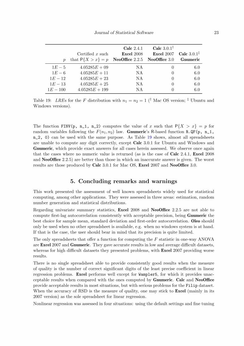
The function FINV(p, n_1, n_2) computes the value of x such that P{X > x} = p forrandom variables following the F (n1, n2) law. Gnumeric’s R-based function R.QF(p, n_1,

n_2, 0) can be used with the same purpose. As Table 19 shows, almost all spreadsheetsare unable to compute any digit correctly, except Calc 3.0.1 for Ubuntu and Windows andGnumeric, which provide exact answers for all cases herein assessed. We observe once againthat the cases where no numeric value is returned (as is the case of Calc 2.4.1, Excel 2008and NeoOffice 2.2.5) are better than those in which an inaccurate answer is given. The worstresults are those produced by Calc 3.0.1 for Mac OS, Excel 2007 and NeoOffice 3.0.

5. Concluding remarks and warnings

This work presented the assessment of well known spreadsheets widely used for statisticalcomputing, among other applications. They were assessed in three areas: estimation, randomnumber generation and statistical distributions.

Regarding univariate summary statistics, Excel 2008 and NeoOffice 2.2.5 are not able tocompute first-lag autocorrelation consistently with acceptable precision, being Gnumeric thebest choice for sample mean, standard deviation and first-order autocorrelation. Oleo shouldonly be used when no other spreadsheet is available, e.g. when no windows system is at hand.If that is the case, the user should bear in mind that its precision is quite limited.

The only spreadsheets that offer a function for computing the F statistic in one-way ANOVAare Excel 2007 and Gnumeric. They gave accurate results in low and average difficult datasets,whereas for high difficult datasets they presented problems, with Excel 2007 providing worseresults.

There is no single spreadsheet able to provide consistently good results when the measureof quality is the number of correct significant digits of the least precise coefficient in linearregression problems. Excel performs well except for Wampler5, for which it provides unac-ceptable results when compared with the ones computed by Gnumeric. Calc and NeoOfficeprovide acceptable results in most situations, but with serious problems for the Filip dataset.When the accuracy of RSD is the measure of quality, one may stick to Excel (mainly in its2007 version) as the sole spreadsheet for linear regression.

Nonlinear regression was assessed in four situations: using the default settings and fine tuning


the parameters, with two starting points for each one, namely, close and far from the certifiedsolution. Using the default settings and both starting points, though some algorithms pre-sented good results in more than half datasets, serious problems were observed with the rest.The DEPS algorithm presented the best success/failure rate, but it did not produce reliableresults in more than 30% of the cases; therefore, there is not enough evidence to advise itsuse for nonlinear regression. Moreover, Calc 2.4.1 and NeoOffice 2.2.5 should not be used forthis purpose. Calc 2.4.1 and NeoOffice 2.2.5 do not provide means for adjusting the algo-rithms parameters, a major drawback for serious users. An overall better behavior is observedwith tuned parameters, and differences are noticed between starting points. Regarding theremaining spreadsheets, at least one (two, resp.) digit(s) of accuracy for the first (second,resp.) starting point is (are) not achieved in only four datasets. DEPS again achieves the bestresults with more than 70% of reliable results, followed by Newton; Conjugate fails in morethan 70% of the assessments, while SCO fails in more than 65% (50%, resp.) with the first(second, resp.) start point. When starting in the optimal solution, Conjugate and Newtonfail only once in identifying that they already are at the solution. Therefore, there is still notenough evidence to advise their use for nonlinear regression, since they fail in almost 30% ofthe cases, in the best situations.

Whichever the spreadsheet and platform, issues regarding documentation and/or repeatabilityprevent their use in serious statistical procedures that employ simulation.

Concerning distribution functions, cases that pose difficulties, identified by Yalta (2008), wereassessed. For all the situations Gnumeric achieved exact answers. Similarly, Calc 3.0.1 forUbuntu and Windows achieved good precision, except for the Poisson cumulative distributionfunction. The binomial distribution should not be computed with Excel 2007. Excel hasserious problems with the Poisson distribution, and its precision is limited for the standardGaussian distribution. Calc 3.0.1, NeoOffice 3.0 and Gnumeric offer good results for the betadistribution. Only Calc 3.0.1 for Ubuntu and Windows and Gnumeric should be used for thet and F distributions.

There are some variations of LRE values in the same platforms when evaluated in differentoperating systems and architectures. However, those variations are not significative, with theexception of Excel 2008 and Calc 3.0.1 for Mac OS. The former presents improved LRE valuesfor binomial distribution, but worse results when calculating the sample standard deviation.In Calc 3.0.1, the Mac OS version presents significantly worse results for t and F distributionsthan its Ubuntu and Windows versions.

On the other hand, improvements were observed for some distribution functions. Calc 3.0.1and NeoOffice 3.0 enhanced their precision, when compared to previous versions, regardingthe χ2 and beta distributions.

Summarizing the main points herein discussed, it is not recommended to use any spreadsheetfor nonlinear regression and/or Monte Carlo experiments. Excel incurs in the very sameerrors of older versions detected, among others, by McCullough (2008b); McCullough andHeiser (2008); McCullough (2004); Nash (2008). Nash (2008) claims that no spreadsheetshould be used in classroom, especially for teaching statistics.

Concerning graphics production, McCullough and Heiser (2008) and Su (2008) argue that thedefault charts produced by Excel do not promote data comprehension, and may cause prob-lems in their understanding. No assessment of the quality of charts produced by spreadsheetsother than Excel was found in the literature, and this is a venue for future research.


Regarding costs, spreadsheets distributed under the terms of the GPL/LGPL, namely, Calc,Gnumeric, NeoOffice and Oleo, can be freely used and distributed. Excel’s license has to bepurchased.

Finally, as a rule of the thumb, every user should be aware that spreadsheets have seriouslimitations. Other platforms are advisable, being currently R the most dependable FLOSS(Free/Libre Open Source Software, see Almiron et al. 2009).

Acknowledgments

The authors thank CAPES, CNPq and FAPEAL for supporting this research, and alsoProf. Francisco Cribari-Neto (Departamento de Estatıstica, Universidade Federal de Pernam-buco, Brazil) for his useful comments and insights. The reviewers provided useful suggestionsthat led to an extended and improved version of the first manuscript. We are also grateful toProf. Bruce D. McCullough (Department of Decision Sciences and Department of Economics,Drexel University, Philadelphia) for making available his spreadsheet files.

References

Aliane N (2008). “Spreadsheet-Based Control System Analysis and Design – A Command-Oriented Toolbox for Education.” IEEE Control Systems Magazine, 28(5), 108–113.

Almiron MG, Almeida ES, Miranda MN (2009). “The Reliability of Statistical Functionsin Four Software Packages Freely Used in Numerical Computation.” Brazilian Journal ofProbability and Statistics, 23(2), 107–119.

Altman M (2002). “A Review of JMP 4.03 with Special Attention to Its Numerical Accuracy.”The American Statistician, 56(1), 72–75.

Apigian CH, Gambill SE (2004). “Is Microsoft Excel 2003 Ready for the Statistics Classroom?”Journal of Computer Information Systems, 45(2), 27–35.

Backman S (2008). “Microeconomics Using Excel: Integrating Economic Theory, Policy Anal-ysis and Spreadsheet Modelling.” European Review of Agricultural Economics, 35(2), 247–248.

Berger RL (2007). “Nonstandard Operator Precedence in Excel.” Computational Statistics &Data Analysis, 51(6), 2788–2791.

Bianchi C, Botta F, Conte L, Vanoli P, Cerizza L (2008). “Biological Effective Dose Evaluationin Gynaecological Brachytherapy: LDR and HDR Treatments, Dependence on Radiobio-logical Parameters, and Treatment Optimisation.” Radiologia Medica, 113(7), 1068–1078.

Bustos OH, Frery AC (2006). “Statistical Functions and Procedures in IDL 5.6 and 6.0.”Computational Statistics & Data Analysis, 50(2), 301–310.

Croll GJ (2009). “Spreadsheets and the Financial Collapse.” In Proceedings of the EuropeanSpreadsheet Risks Interest Group, pp. 145–161.


Dzik WS, Beckman N, Selleng K, Heddle N, Szczepiorkowski Z, Wendel S, Murphy M (2008).“Errors in Patient Specimen Collection: Application of Statistical Process Control.” Trans-fusion, 48(10), 2143–2151.

Free Software Foundation (2000). GNU Oleo 1.99.16. Free Software Foundation, Inc., Boston,MA. URL http://www.gnu.org/software/oleo/.

Free Software Foundation (2007a). “GNU General Public License.” URL http://www.gnu.

org/copyleft/gpl.html.

Free Software Foundation (2007b). “GNU Lesser General Public License.” URL http://www.

gnu.org/licenses/lgpl.html.

Galassi M, Davies J, Theiler J, Gough B, Jungman G, Booth M, Rossi F (2003). GNUScientific Library Reference Manual. 2nd edition. Network Theory Ltd.

Heiser D (2006). “Microsoft Excel 2000 and 2003 Faults, Problems, Workarounds and Fixes.”Computational Statistics & Data Analysis, 51(2), 1442–1443.

Kaiser J (2002). “Air Pollution Risks – Software Glitch Threw Off Mortality Estimates.”Science, 296(5575), 1945–1947.

Keeling KB, Pavur RJ (2007). “A Comparative Study of the Reliability of Nine StatisticalSoftware Packages.” Computational Statistics & Data Analysis, 51(8), 3811–3831.

Kennedy WJ, Gentle JE (1980). Statistical Computing. Marcel Dekker, New York, NY.

Knight J (2002). “Statistical Error Leaves Pollution Data Up in the Air.” Nature, 417(6890),677–677.

Knusel L (1995). “On the Accuracy of the Statistical Distributions in GAUSS.” ComputationalStatistics & Data Analysis, 20(6), 699–702.

Knusel L (1998). “On the Accuracy of Statistical Distributions in Microsoft Excel 97.” Com-putational Statistics & Data Analysis, 26(3), 375–377.

Knusel L (2005). “On the Accuracy of Statistical Distributions in Microsoft Excel 2003.”Computational Statistics & Data Analysis, 48(3), 445–449.

Knuth DE (1998). The Art of Computer Programming, volume II / Seminumerical Algorithms.3rd edition. Addison-Wesley.

Kruck SE (2006). “Testing Spreadsheet Accuracy Theory.” Information and Software Tech-nology, 48(3), 204–213.

Lindstrom RM, Asvavijnijkulchai C (1998). “Ensuring Accuracy in Spreadsheet Calculations.”Fresenius Journal of Analytical Chemistry, 360(3–4), 374–375.

Marsaglia G (1995). “The Marsaglia Random Number CDROM, Including the Diehard Bat-tery of Tests of Randomness.” Master copy at http://stat.fsu.edu/pub/diehard/. Im-proved version at http://www.cs.hku.hk/~diehard/.

http://www.gnu.org/software/oleo/

http://www.gnu.org/copyleft/gpl.html

http://www.gnu.org/copyleft/gpl.html

http://www.gnu.org/licenses/lgpl.html

http://www.gnu.org/licenses/lgpl.html

http://stat.fsu.edu/pub/diehard/

http://www.cs.hku.hk/~diehard/


Matsumoto M, Nishimura T (1998). “Mersenne Twister: A 623-Dimensionally EquidistributedUniform Pseudo-Random Number Generator.” ACM Transactions on Modeling and Com-puter Simulation, 8(1), 3–30.

McCullough BD (1998). “Assessing the Reliability of Statistical Software: Part I.” TheAmerican Statistician, 52(4), 358–366.

McCullough BD (1999). “Assessing the Reliability of Statistical Software: Part II.” TheAmerican Statistician, 53(2), 149–159.

McCullough BD (2000). “Is It Safe to Assume that Software Is Accurate?” InternationalJournal of Forecasting, 16(3), 349–357.

McCullough BD (2004). “Fixing Statistical Errors in Spreadsheet Software: The Cases of Gnu-meric and Excel.” Computational Statistics & Data Analysis Statistical Software Newsletter,pp. 1–10.

McCullough BD (2008a). “Microsoft Excel’s ‘Not the Wichmann-Hill’ Random Number Gen-erators.” Computational Statistics & Data Analysis, 52(10), 4587–4593.

McCullough BD (2008b). “Special Section on Microsoft Excel 2007.” Computational Statistics& Data Analysis, 52(10), 4568–4569.

McCullough BD, Heiser DA (2008). “On the Accuracy of Statistical Procedures in MicrosoftExcel 2007.” Computational Statistics & Data Analysis, 52(10), 4570–4578.

McCullough BD, Wilson B (1999). “On the Accuracy of Statistical Procedures in MicrosoftExcel 97.” Computational Statistics & Data Analysis, 31(1), 27–37.

McCullough BD, Wilson B (2002). “On the Accuracy of Statistical Procedures in MicrosoftExcel 2000 and Excel XP.” Computational Statistics & Data Analysis, 40(4), 713–721.

McCullough BD, Wilson B (2005). “On the Accuracy of Statistical Procedures in MicrosoftExcel 2003.” Computational Statistics & Data Analysis, 49(4), 1244–1252.

Microsoft Corporation (2007). Microsoft Office Excel 2007. URL http://office.

microsoft.com/excel.

Nash JC (2006). “Spreadsheets in Statistical Practice – Another Look.” The AmericanStatistician, 60(3), 287–289.

Nash JC (2008). “Teaching Statistics with Excel 2007 and Other Spreadsheets.” Computa-tional Statistics & Data Analysis, 52(10), 4602–4606.

National Institute of Standards and Technology (1999). “Statistical Reference Datasets:Archives.” URL http://www.itl.nist.gov/div898/strd/general/dataarchive.html.

Ozkaya SI (1996). “An Excel Macro for Importing Log ASCII Standard (LAS) Files intoExcel Worksheets.” Computers & Geosciences, 22(1), 75–80.

Planamesa, Inc (2009). NeoOffice 3.0. URL http://www.NeoOffice.org/.

http://office.microsoft.com/excel

http://office.microsoft.com/excel

http://www.itl.nist.gov/div898/strd/general/dataarchive.html

http://www.NeoOffice.org/


Powell SG, Baker KR, Lawson B (2009). “Impact of Errors in Operational Spreadsheets.”Decision Support Systems, 47, 126–132.

R Development Core Team (2009). R: A Language and Environment for Statistical Computing.R Foundation for Statistical Computing, Vienna, Austria. ISBN 3-900051-07-0, URL http:

//www.R-project.org/.

Ripley BD (1987). Stochastic Simulation. John Wiley & Sons, New York, NY.

Ripley BD (1990). “Thoughts on Pseudorandom Number Generators.” Journal of Computa-tional and Applied Mathematics, 31, 153–163.

Roth J (2008). “Ergebnisse von Qualitatskontrollen der Individuellen Patientendosen in derRadioonkologie.” Strahlentherapie und Onkologie, 184(10), 505–509.

Rukhin A, Soto J, Nechvatal J, Smid M, Barker E, Leigh S, Levenson M, Vangel M, Banks D,Heckert A, Dray J, Vo S (2008). A Statistical Test Suite for Random and PseudorandomNumber Generators for Cryptographic Applications. National Institute of Standards andTechnology. NIST Special Publication 800-22rev1, URL http://csrc.nist.gov/groups/

ST/toolkit/rng/.

Segaran T, Hammerbacher J (eds.) (2009). Beaultiful Data. O’Reilly.

Simon SD, Lesage JP (1989). “Assessing the Accuracy of ANOVA Calculations in StatisticalSoftware.” Computational Statistics & Data Analysis, 8(3), 325–332.

Su Y (2008). “It’s Easy to Produce Chartjunk Using Microsoft Excel 2007 but Hard to MakeGood Graphs.” Computational Statistics & Data Analysis, 52(10), 4594–4601.

Sun Microsystems Inc (2009). OpenOffice.org Calc 3.0.1. URL http://www.OpenOffice.

org/.

The Gnumeric Team (2007). The Gnumeric Manual, Version 1.8. GNOME DocumentationProject. URL http://projects.gnome.org/gnumeric/.

Vinod HD (2000). “Review of GAUSS for Windows, Including Its Numerical Accuracy.”Journal of Applied Econometrics, 15(2), 211–220.

Wichmann BA, Hill ID (1982). “Algorithm AS 183: An Efficient and Portable Pseudo-RandomNumber Generator.” Applied Statistics, 31(2), 188–190.

Wichmann BA, Hill ID (2006). “Generating Good Pseudo-Random Numbers.” ComputationalStatistics & Data Analysis, 51(3), 1614–1622.

Xie XF, Zhang WJ, Yang ZL (2002). “Social Cognitive Optimization for Nonlinear Program-ming Problems.” In Proceedings of the First International Conference on Machine Learningand Cybernetics, volume 2, pp. 779–783.

Yalta AT (2007). “The Numerical Reliability of GAUSS 8.0.” The American Statistician,61(3), 262–268.

Yalta AT (2008). “The Accuracy of Statistical Distributions in Microsoft Excel 2007.” Com-putational Statistics & Data Analysis, 52(10), 4579–4586.

http://www.R-project.org/

http://www.R-project.org/

http://csrc.nist.gov/groups/ST/toolkit/rng/

http://csrc.nist.gov/groups/ST/toolkit/rng/

http://www.OpenOffice.org/

http://www.OpenOffice.org/

http://projects.gnome.org/gnumeric/


Yalta AT, Yalta AY (2007). “GRETL 1.6.0 and Its Numerical Accuracy.” Journal of AppliedEconometrics, 22(4), 849–854.

Zhang WJ, Xie XF (2003). “DEPSO: Hybrid Particle Swarm with Differential EvolutionOperator.” In IEEE International Conference on Systems, Man and Cybernetics, volume 4,pp. 3816–3821.

Zoethout RWM, van Gerven JMA, Dumont GJH, Paltansing S, van Burgel ND, van derLinden M, Dahan A, Cohen AF, Schoemaker RC (2008). “A Comparative Study of TwoMethods for Attaining Constant Alcohol Levels.” British Journal of Clinical Pharmacology,66(5), 674–681.

Affiliation:

Alejandro C. FreryInstituto de ComputacaoLCCV & CPMATUniversidade Federal de AlagoasBR 104 Norte km 9757072–970 Maceio, AL, BrazilE-mail: [email protected]

Journal of Statistical Software http://www.jstatsoft.org/

published by the American Statistical Association http://www.amstat.org/

Volume 34, Issue 4 Submitted: 2008-12-11April 2010 Accepted: 2010-01-31

mailto:[email protected]

http://www.jstatsoft.org/

http://www.amstat.org/

On the Numerical Accuracy of Spreadsheets

Documents

Transcript of On the Numerical Accuracy of Spreadsheets