On the Moebius Trigonometric Polynomial -...

On the Moebius Trigonometric Polynomial

Olivier Ramaré

CNRS, Laboratoire Paul Painlevé,Université Lille 1, 59 655 Villeneuve d’Ascq, France

Email: [email protected]

April 2, 2014

Abstract

File MoebiusTalk-2.tex.

1. A preliminary stroll

In 1937, Harold Davenport1 was newly appointed at the University of Manch-ester, where Louis Mordell had also a chair. H.Davenport proved in [Davenport,1937a] and among other things2 that

(1.1)∞∑n=1

µ(n)

nnθ = − sin 2πθ

π(a.e.)

2010 Mathematics Subject Classification: Primary , ; Secondary .Key words and phrases:

1H. Davenport was a student of J.E. Littlewood. He graduated in 1927, but got his thesisfrom Cambridge in 1937 only.

2The Riemann zeta function is defined for <s > 1 by ζ(s) =∑

n≥1 1/ns. It also verifies

ζ(s) =∏

p≥2

(1 − p−s

)−1 where the product is absolutely convergent in the [strong] senseof Godement and the variable p ranges over the primes. We deduce from that that ζ(s)1 =∑

n≥1 µ(n)/ns for a function µ(n) named after the german mathematician Auguste Moebius

who studied it more systematically in 1832 (but this function appears already in Euler in 1748or in Gauss’s Disquisitiones arithmeticae from 1801). We have

∑d|n µ(d) = 1n=1, almost by

definition. The fact that∑

n≥1 µ(n)/n is known to be “equivalent” to the prime numbertheorem, this was E. Landau’s phd thesis in 1899 in fact, but the term “equivalent” maysound strange between two results that are ... true! Such a statement may be quantified andit is the purpose of [Kienast, 1926] and more recently of [Ramaré, 2013]. In terms of Dirichletseries, we have −ζ′(s)/ζ(s) =

∑p≥2 log(p)/(p

s − 1).

2

for almost every θ. Giving a formal proof is easy enough: we use u − 12 =

−∑h≥1 sin(2πhu)/(πh), valid when h is not an integer, and get

∞∑n=1

µ(n)

nnθ =

∞∑n=1

µ(n)

n

(nθ − 1

2

)= −

∑n≥1

µ(n)

n

∑h≥1

sin(2πnhθ)

πh

= −∑m≥1

( ∑nh=m

µ(n)) sin(2πmθ)

πm= − sin(2πθ)

π.

but how can one actually prove the identity above? Let us introduce the notation(from Davenport’s paper)

(1.2) RN (θ) =∑

1≤n≤N

µ(n)

nnθ+

sin 2πθ

π.

H. Davenport first notices a property that enables one to go from a single valueto an average sum1.

Lemma 1 We have RN (θ2) − RN (θ1) N |θ2 − θ1| + (logN)−h, forarbitrary N , θ2, θ1 and h.

We use the usual notation for the Bernoulli periodical functions ψ1(x) =x − 1

2 and ψ2(x) = x2 − x+ 16 so that

2

∫ x

0

ψ1(t)dt = ψ2(x)− 16 , ψ2(x) = −

∑k≥1

cos 2πkx

π2k2.

We define

(1.3) TN (θ) =∑n>N

µ(n)

2n2ψ2(nθ).

The next Lemma reduces the problem to estimating TN (θ).

Lemma 2∫ θ2

θ1

RN (θ)dθ = TN (θ1)− TN (θ2) +∑

1≤n≤N

µ(n)(θ2 − θ1)

2n.

We can now write

TN (θ) =∑k≥1

1

2π2k2

∑n>N

µ(n) cos 2πknθ

n2

1A simple but tricky, tricky proof!

April 2, 2014 Version 1

1 Expectations 3

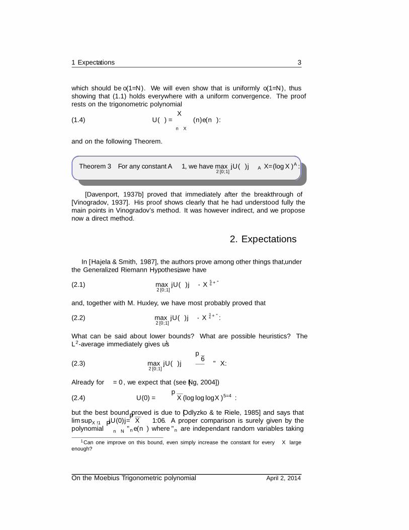
which should be o(1/N). We will even show that is uniformly o(1/N), thusshowing that (1.1) holds everywhere with a uniform convergence. The proofrests on the trigonometric polynomial

(1.4) U(α) =∑n≤X

µ(n)e(nα).

and on the following Theorem.

Theorem 3 For any constant A ≥ 1, we have maxα∈[0,1]

|U(α)| A X/(logX)A.

[Davenport, 1937b] proved that immediately after the breakthrough of[Vinogradov, 1937]. His proof shows clearly that he had understood fully themain points in Vinogradov’s method. It was however indirect, and we proposenow a direct method.

2. Expectations

In [Hajela & Smith, 1987], the authors prove among other things that, underthe Generalized Riemann Hypothesis, we have

(2.1) maxα∈[0,1]

|U(α)| ε X56+ε

and, together with M. Huxley, we have most probably proved that

(2.2) maxα∈[0,1]

|U(α)| ε X34+ε.

What can be said about lower bounds? What are possible heuristics? TheL2-average immediately gives us1

(2.3) maxα∈[0,1]

|U(α)| ≥(√6

π− ε)X.

Already for α = 0, we expect that (see [Ng, 2004])

(2.4) U(0) = Ω±(√X(log log logX)5/4

).

but the best bound proved is due to [Odlyzko & te Riele, 1985] and says thatlim supX→∞ |U(0)|/

√X ≥ 1.06. A proper comparison is surely given by the

polynomial∑n≤N εne(nθ) where εn are independant random variables taking

1Can one improve on this bound, even simply increase the constant for every X largeenough?

On the Moebius Trigonometric polynomial April 2, 2014

4

the values ±1 with equal probability. [Halász, 1973], following [Salem & Zyg-mund, 1954], shows that in such circumstances, the maximum is asymptotic to√X logX. This constitutes ground for the conjecture:

maxα∈[0,1]

|U(α)|?√X logX

The litterature on this trigonometric polynomial is not very dense, and wemention [Codecà & Nair, 2000, Theorem 3], [Hajela & Smith, 1987, Theorem2.1] and [Iwaniec & Kowalski, 2004, Theorem 13.9]. The L1-mean has also beenconsidered in [Balog & Ruzsa, 1999] and [Balog & Ruzsa, 2001] (the corre-sponding problem on the primes has received a much more satisfactory answerin [Vaughan, 1988]). There has been recently some more interest for this prob-lem [Bourgain et al., 2012].

3. Splitting the circle

We partition the circle R/Z in neighborhoods of rational points by appealingto the Dirichlet Theorem. Every α ∈ R/Z can be written in the following form:

(3.1) α =a

q+ β, q ≤ Q, (a, q) = 1, |β| ≤ 1

qQ

where Q = X/(logX)2A+7, the constant A being the one from Theorem 3. Theresult may be uniform, the proof is not uniform! There are three main times:

• The arithmetical time. By arithmetical here, we mean informationon the distribution of the Moebius function when the variable belongs tosome arithmetic progression.

• The Fourier analysis time. This will extend the information obtainedvia arithmetic to some neighbourhood.

• The combinatorial time. The previous part took take of the first har-monics, in a vague sense, and we have to control the noise. This is themain novelty.

4. The arithmetical time

The treatment of the q ≤ (logX)2A+7 uses the zero-free region of the Dirich-let L-functions and a classical analysis shows the following. Let C1 and C2 betwo positive constants. For every Dirichlet (not necessarily primitive) characterχ of modulus q ≤ (logX)C1 , we have

(4.1)∑n≤X

µ(n)χ(n)C1,C2 X/(logX)C2 .


4 The Fourier analysis time 5

We infer the following.

Lemma 4 For every positive constants C1 and C3, for every b and everyq ≤ (logX)C1 , we have

(4.2)∑n≤X,

(n,q)=1

µ(n)e(nb/q)C1,C3 X/(logX)C3 .

We next remove the condition (n, q) = 1 that appears in (4.2).

Lemma 5 We have, for any C1, C4 ≥ 1 and every q ≤ (logX)C1 ,

(4.3)∑n≤X

µ(n)e(na/q)c1,C4 X/(logX)C4 .

We will select C4 = 3A+ 7.

5. The Fourier analysis time

The next step is to extend the estimate of Lemma 5 to nearby values. Themanner to do so is classical within the framework of the circle method and oneshould retain the principle: if we know

∑n≤Y h(n) not only in Y = X, but also

for nearby values of Y (here between X/(logX)C and X), then we can extendthe bound to

∑n≤Y h(n)e(βn) for β = 0 to small βs.

Lemma 6 We have, for A,C ≥ 1 and q ≤ (logX)2A+7,

(5.1)∑n≤X

µ(n)e

(n(aq

+ β)) X/(logX)A.

provided that |qβ| ≤ 1/Q.

6. The combinatorial time

Here is the Theorem we will need.


6

Theorem 7 a Let α be a point of R/Z. We assume given two positive realparameters X ≥ Q ≥ 2 and a rational number a/q such that |qα−a| ≤ 1/Qand q ≤ Q. We have∣∣∣∑

n≤X

µ(n)e(nα)∣∣∣ ≤ 30X√

min(q,X/q,√Q)

(1 + logX)7/2.

aIt improves on [Codecà & Nair, 2000, Theorem 3], [Hajela & Smith, 1987, Theorem2.1] and [Iwaniec & Kowalski, 2004, Theorem 13.9].

The identity (‡) used here comes from [Vaughan, 1977], and happens also to bea simplified version of the one proven in [Ramaré, 2013].

The parameter X from the Theorem is large and given. We select anotherparameter, z, that we will choose below in choice (6.12). Here the hypothesiswe make:

(6.1) z ≤ q ≤ X/z , z2 ≤ Q/2 and X/z ≤ Q/4.

We however keep this parameter it unspecified and optimize it at the end. Apossible value is z = X1/5 since Q will be typically of size X1−ε. We use herethe following function:

(6.2) µz(d) =

µ(d) when d ≤ z,0 else.

We also specify a notation for its Dirichlet series:

(6.3) Mz(s) =∑d≤z

µ(d)

ds.

6.1 An identity

The most conceptual proof runs as follows. We define

(6.4) V (s) =∑n≥2

(∑d|n

µz(d))/ns =

∑n≥2

v(n)/ns.

Notice that n ranges over the integers that are greater than z. This series almostfactors:

(6.5) 1 + V (s) = ζ(s)M(s)

Here is the formal decomposition of 1 that we will use:

1 = −V + ζMz.


6.2 Treating the linear sum 7

On using this, we decompose 1/ζ as follow:

1

ζ= −1

ζV +Mz.

The work is almost over but we still have to refine the decomposition and put(ζ−1 −Mz) in the first factor. This is easily done

1

ζ= −

(1

ζ−Mz

)V −MzV +Mz

and finally, by using again V = Mzζ − 1,

(6.6)1

ζ= −

(1

ζ−Mz

)V −M2

z ζ + 2Mz.

We can translate this identity on the Moebius function by equating the coeffi-cients of the corresponding Dirichlet series and get1:

( (‡) µ = −(µ− µz) ? v − µz ? µz ? 1 + 2µz.

This identity enables us to write

(6.7)∑n≤X

µ(n)e(nα) = −∑n≤X

((µ− µz) ? v

)(n)e(nα)

+∑n≤X

(µz ? µz ? 1)(n)e(nα) + 2∑n≤z

µ(n)e(nα).

The combinatorial input ends here and we now study each sum independently.The first sum is said to be bilinear, a name due to the way it is studied, or of

type II by Vinogradov; the second one is said linear, or of type I by Vinogradov,while the third one is simply a remainder term, here bounded in absolute valueby 2z. The function n 7→ (µ−µz)∗v(n) is fully unknown, but we are going to useonly its shape as a convolution product over localized divisors of not-too-largefunctions.

6.2 Treating the linear sum

Lemma 8∣∣∣∣∑d≤z2

(µz ? µz)(d)∑

m≤X/d

e(dmα)

∣∣∣∣ ≤ 2X√q

(1 + 2 log z)2 + z2q.

1The reader could have also simply developped (1?µz−e)?(µ−µz) where e is the neutralelement of the arithmetical convolution product: this function takes value 1 at n = 1 and 0everywhere else (its Dirichlet series is simply the constant function equal to 1).


8

Proof. We start with∑n≤X

(µz ? µz ? 1)(n)e(nα) =∑d≤z2

(µz ? µz)(d)∑

m≤X/d

e(dmα).

Since z2 ≤ Q/2 by (6.1), we have |dα − daq | ≤

12q . When q - d, we simply sum

the inner geometric progression and get

(6.8)∣∣∣ ∑m≤X/d

e(dmα)∣∣∣ ≤ 1/| sin(πdα)| ≤ 1/‖da/q‖ ≤ q

where ‖α‖ is the distance to the closest integer and where we have used theclassical inequality

1

sin(πx)≤ 1

2x(0 < x ≤ 1/2).

We continue with∑d≤z2 |(µz ? µz)(d)| ≤ z2. This finally amount to the contri-

bution:

(6.9)∣∣∣∣ ∑d≤z2,q-d

(µz ? µz)(d)∑

m≤X/d

e(dmα)

∣∣∣∣ ≤ z2q.When q|d, we bound trivially e(dmα) by 1, i.e. we use∣∣∣ ∑

m≤X/d

e(dmα)∣∣∣ ≤ X/d.

Hence1 ∣∣∣∣ ∑d≤z2,q|d

(µz ? µz)(d)∑

m≤X/d

e(dmα)

∣∣∣∣ ≤ X ∑d≤z2,q|d

τ(d)

d.

We use the simple inequalities τ(q`) ≤ τ(q)τ(`) and τ(q) ≤ 2√q together with

∑d≤z2,q|d

τ(d)

d≤ τ(q)

q

∑`≤z2/q

τ(`)

`≤ τ(q)

q(1 + 2 log z)2

≤ 2√q

(1 + 2 log z)2

1The number τ(d) is the number of (positive) divisors of d.


6.3 Treating the bilinear sum 9

since we readily check that

(6.10)∑`≤L

τ(`)

`≤(∑m≤L

1

m

)2

≤ (1 + logL)2.

Note that we may have z2/q < 1 above, but the bound∑`≤z2/q

τ(`)` ≤ (1 +

2 log z)2 holds nonetheless. All of that amounts to

(6.11)∣∣∣∣ ∑d≤z2,q|d

(µz ? µz)(d)∑

m≤X/d

e(dmα)

∣∣∣∣ ≤ 2X√q

(1 + 2 log z)2.

We combine (6.9) and (6.11) to conclude.

6.3 Treating the bilinear sumThe previous part do not require anything in particular and could have beendone well before Vinogradov’s time. What this latter brought is (one) the recog-nition of the bilinear sums and (two) the way they can be treated. Vinogradovexplains that fully in the introduction of his book [Vinogradov, 2004]. He willfurther use the very same technique to study exponential sums with polynomialphases. Said in simplistic terms, the idea is to use the Cauchy inequality, whichhas the effect of creating a smooth variable over which we can sum a geometricseries. To be able to employ the Cauchy inequality with a minimum amount ofloss, we first have to have sums of similar lengths, and since this length is ruledby X/m in the left-hand part of (6.13), we need m to be about of constant size.The proof has three steps:

• A diadic decomposition.

• Using Cauchy’s inequality.

• Treating the diagonal and off-diagonal terms separately.

Here is the fundamental result we prove.

Lemma 9 ∑n≤X

µ(n)e(nα) ≤ 15X√z

(1 + logX)7/2.

Theorem 3 follows by chosing

(6.12) z = min(q,X/q,√Q)/4

which indeed verifies (6.1).


10

Proof.

Diadic decompositionWe readily show that1

(6.13)

∣∣∣∣∣ ∑dm≤X,d>z

µ(d)v(m)e(dmα)

∣∣∣∣∣≤ 3(logX) max

z≤M≤X/z,M≤M ′≤min(2M,X/z)

∣∣∣∣∣ ∑dm≤X,

M≤m≤M ′,d>z

µ(d)v(m)e(dmα)

∣∣∣∣∣.

Or, when expressed in a shorter way: if we are ready to loose a factor logX, wecan localize the variable m. We could also localize the variable d, by starting atthe very beginning with the sum

∑X/2<n≤X µ(n)e(nα). This is not required in

the simplistic treatment we propose here.

Using the Cauchy inequalityWe first sum on the m-variable and apply the Cauchy inequality, i.e. we

write∣∣∣∣∣ ∑dm≤X,

M≤m≤M ′,d>z

µ(d)v(m)e(dmα)

∣∣∣∣∣2

≤∑

M≤m≤M ′

|v(m)|2

×∑

z<d1,d2≤ XM

µ(d1)µ(d2)∑

m∈I(d1,d2)

e((d1 − d2)mα).

where I(d1, d2) is the interval [M,min(M ′, X/max(d1, d2))]. This interval con-tains at mostM +1 integer points. The announced phenomenom occurs: in thesecond sum, the m-variable is now smooth, by which we mean that its coefficientdoes not have any arithmetical part anymore (and does not vary abnormallyfast). We are left with a geometric series2.

1Since 1 + (logX)/ log 2 ≤ 3 logX when X ≥ 2.2Here is a parenthesis concerning

∑M≤m≤M′ |v(m)|2. We have (on following a path

similar to (6.10) since |v(m)| ≤ τ(m))∑M≤m≤M′

|v(m)|2 ≤M ′∑

m≤M′

|v(m)|2

m≤M ′

∑m≤M′

τ(m)2

m

≤M ′∑

d1,d2≤M′

τ(d1d2)

d1d2≤M ′

∑d1,d2≤M′

τ(d1)τ(d2)

d1d2

≤M ′ ∑

d1≤M′

τ(d1)

d1

2


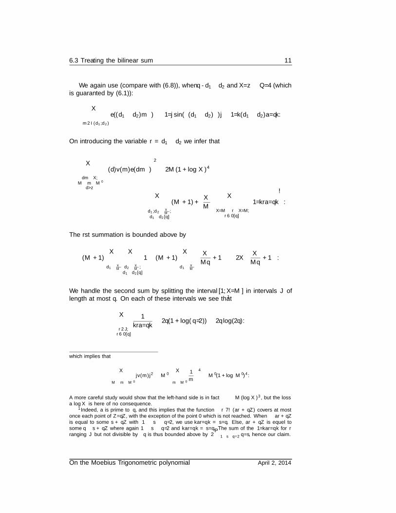
6.3 Treating the bilinear sum 11

We again use (compare with (6.8)), when q - d1− d2 and X/z ≤ Q/4 (whichis guaranted by (6.1)):

∣∣∣ ∑m∈I(d1,d2)

e((d1 − d2)mα)∣∣∣ ≤ 1/| sin(π(d1 − d2)α)| ≤ 1/‖(d1 − d2)a/q‖.

On introducing the variable r = d1 − d2 we infer that

∣∣∣∣∣ ∑dm≤X,

M≤m≤M ′

d>z

µ(d)v(m)e(dmα)

∣∣∣∣∣2

≤ 2M(1 + logX)4

×

( ∑d1,d2≤ X

M ,d1≡d2[q]

(M + 1) +X

M

∑−X/M≤r≤X/M,

r 6≡0[q]

1/‖ra/q‖

).

The first summation is bounded above by

(M + 1)∑d1≤ X

M

∑d2≤ X

M ,d1≡d2[q]

1 ≤ (M + 1)∑d1≤ X

M

(X

Mq+ 1

)≤ 2X

(X

Mq+ 1

).

We handle the second sum by splitting the interval [1, X/M ] in intervals J oflength at most q. On each of these intervals we see that1

∑r∈J,r 6≡0[q]

1

‖ra/q‖≤ 2q(1 + log(q/2)) ≤ 2q log(2q).

which implies that

∑M≤m≤M′

|v(m)|2 ≤M ′( ∑

m≤M′

1

m

)4

≤M ′(1 + logM ′)4.

A more careful study would show that the left-hand side is in fact M(logX)3, but the lossa logX is here of no consequence.

1Indeed, a is prime to q, and this implies that the function r 7→ (ar + qZ) covers at mostonce each point of Z/qZ, with the exception of the point 0 which is not reached. When ar+qZis equal to some s + qZ with 1 ≤ s ≤ q/2, we use ‖ar/q‖ = s/q. Else, ar + qZ is equel tosome q − s+ qZ where again 1 ≤ s ≤ q/2 and ‖ar/q‖ = s/q. The sum of the 1/‖ar/q‖ for rranging J but not divisible by q is thus bounded above by 2

∑1≤s≤q/2 q/s, hence our claim.


12

Since there are at most XMq + 1 such intervals J , we have reached

(6.14)

∣∣∣∣∣ ∑dm≤X,

M≤m≤M ′

d>z

µ(d)v(m)e(dmα)

∣∣∣∣∣2

≤ 2M(1 + logX)4

(2X2

Mq+ 2X + 2

X

M

(X

Mq+ 1

)q log(2q)

)

≤ 4

(X2

q+XM +

X2

M+Xq

)(1 + logX)4 log(2q) ≤ 16

X2

z(1 + logX)5.

On carrying (6.14) into (6.13) and adding the rseult of Lemma 8, we see thatwe have proved that1

7. Proof of some Lemmas

Proof. [Proof of Lemma 2] We first notice that∑1≤n≤N

µ(n)

n

∫ θ2

θ1

ψ1(nθ)dθ =∑

1≤n≤N

µ(n)

2n2(ψ2(nθ2)− ψ2(nθ1)).

The second step reads∑n≥1

µ(n)

n2ψ2(nθ) =

∑k,n≥1

µ(n)

π2(nk)2cos(2πknθ) =

cos 2πθ

π2

from which we infer that∑n≤N

µ(n)

2n2ψ2(nθ)− cos 2πθ

2π2= −

∑n>N

µ(n)

2n2ψ2(nθ) = −TN (θ),

say. We now resume the main line of the proof:∫ θ2

θ1

RN (θ)dθ =∑

1≤n≤N

µ(n)

2n2(ψ2(nθ2)− ψ2(nθ1)) +

∑1≤n≤N

µ(n)(θ2 − θ1)

2n

− cos 2πθ22π2

+cos 2πθ1

2π2

= TN (θ1)− TN (θ2) +∑

1≤n≤N

µ(n)(θ2 − θ1)

2n

as announced. The Lemma follows readily.1Note that 1 + 2 log z ≤ 1 + logX.


6 Proof of some Lemmas 13

Proof. [Proof of Lemma 4] We can assume (b, q) = 1 by removing the commonfactor. We then note that

(7.1) fb/q : n 7→

e(na/q) when (n, q) = 1,

0 else,

is periodical of period q and of support the multiplicatif group of Z/qZ. Thisfunction can be written as a linear combination of Dirichlet characters moduloq, and this combination is easy to determine thanks to the hermitian structure.We get

fb/q =∑

χ mod q

1

ϕ(q)

∑n mod q,(n,q)=1

e(nb/q)χ(n)χ

=∑

χ mod q

1

ϕ(q)χ(b)

∑n mod q,(n,q)=1

e(n/q)χ(n)χ,

which shows that the coefficients are of absolute value not more than √q/φ(q)(use the value of the modulus of the Gauss sum). We conclude by selectingC2 = C3 + 1

2C1 in (4.1).

Proof. [Proof of Lemma 5] We write∑n≤X

µ(n)e(na/q) =∑δ|q

∑n≤X,

(n,q)=δ

µ(n)e(na/q)

=∑δ|q

µ(δ)∑

m≤X/δ,(m,q)=1

µ(m)e(mδa/q)

where we can now use (4.2), since we do not assume (a, q) = 1 therein, with theparameters C1 and C3 = C4 + 1 . We get∑

n≤X

µ(n)e(na/q)∑δ|q

X

δ(logX)C3 X

(logX)C4

as soon as q ≤ (logX)C1 .

Proof. [Proof of Lemma 6] The last step is to extend the bound in a/q to theneighbourhood. We use the shortcut h(n) = µ(n)e(na/q). We use the inequality


14

|β| ≤ 1/Q. We get, by using Step number 4 with C4 = 3A+ 7,∑n≤X

h(n)e(nβ) =∑n≤X

h(n)(e(Xβ)− 2iπβ

∫ X

n

e(tβ)dt)

= e(Xβ)∑n≤X

h(n)− 2iπβ

∫ X

1

e(tβ)∑n≤t

h(n)dt

X

(logX)A+

1

Q

∫ X/(logX)2A+4

1

tdt+X2

Q(logX)3A+7 X

(logX)A.

References

Balog, A., & Ruzsa, I. Z. 2001. On the exponential sum over r-free integers.Acta Math. Hungar., 90(3), 219–230.

Balog, Antal, & Ruzsa, Imre Z. 1999. A new lower bound for the L1 mean ofthe exponential sum with the Möbius function. Bull. London Math. Soc.,31(4), 415–418.

Bourgain, J., Sarnak, P., & Ziegler, T. 2012. Distjointness of Moebius fromhorocycle flows. 17pp. arXiv:1110.0992.

Codecà, P., & Nair, M. 2000. A note on a result of Bateman and Chowla. ActaArith., 93(2), 139–148.

Davenport, H. 1937a. On some infinite series involving arithmetical functions.Quart. J. Math., Oxf. Ser., 8, 8–13.

Davenport, H. 1937b. On some infinite series involving arithmetical functions.II. Quart. J. Math., Oxf. Ser., 8, 313–320.

Hajela, D., & Smith, B. 1987. On the maximum of an exponential sum of theMöbius function. Pages 145–164 of: Number theory (New York, 1984–1985). Lecture Notes in Math., vol. 1240. Berlin: Springer.

Halász, G. 1973. On a result of Salem and Zygmund concerning random poly-nomials. Studia Sci. Math. Hungar., 8, 369–377.

Iwaniec, H., & Kowalski, E. 2004. Analytic number theory. American Mathe-matical Society Colloquium Publications. American Mathematical Society,Providence, RI. xii+615 pp.

Kienast, A. 1926. Über die Äquivalenz zweier Ergebnisse der analytischenZahlentheorie. Mathematische Annalen, 95, 427–445. 10.1007/BF01206619.

Ng, Nathan. 2004. The distribution of the summatory function of the Möbiusfunction. Proc. London Math. Soc. (3), 89(2), 361–389.

Odlyzko, A. M., & te Riele, H. J. J. 1985. Disproof of the Mertens conjecture.J. Reine Angew. Math., 357, 138–160.


6 Proof of some Lemmas 15

Ramaré, O. 2013. From explicit estimates for the primes to explicit estimatesfor the Moebius function. Acta Arith., 157(4), 365–379.

Ramaré, O. 2013. A sharp bilinear form decomposition for primes and Moebiusfunction. Submitted, 45pp.

Salem, R., & Zygmund, A. 1954. Some properties of trigonometric series whoseterms have random signs. Acta Math., 91, 245–301.

Vaughan, R. C. 1988. The L1 mean of exponential sums over primes. Bull.London Math. Soc., 20(2), 121–123.

Vaughan, R.C. 1977. Sommes trigonométriques sur les nombres premiers. C. R.Acad. Sci. Paris Sér. A-B, 285(16), A981–A983.

Vinogradov, I.M. 1937. A new estimate of a certain sum containing primes.

Vinogradov, I.M. 2004. The method of trigonometrical sums in the theory ofnumbers. Mineola, NY: Dover Publications Inc. Translated from the Rus-sian, revised and annotated by K. F. Roth and Anne Davenport, Reprintof the 1954 translation.


On the Moebius Trigonometric Polynomial -...

Documents

Transcript of On the Moebius Trigonometric Polynomial -...