On the Modular Modelling for Dynamical Simulation with Application to Fluid Systems

TRITA – MMK 2005:30ISSN 1400-1179

ISRN/KTH/MMK/R-05/30-SE

Licentiate thesis Department of Machine Design Royal Institute of Technology SE-100 44 Stockholm

CARL-JOHAN SJÖSTEDT

TRITA – MMK 2005:30 ISSN 1400-1179 ISRN/KTH/MMK/R-05/30-SE

On the Modular Modelling for Dynamical Simulation with Application to Fluid Systems

Carl-Johan Sjöstedt

Licentiate thesis

Academic thesis, which with the approval of Kungliga Tekniska Högskolan, will be presentedfor public review in fulfilment of the requirements for a Licentiate of Engineering in Machine Design. The public review is held at Kungliga Tekniska Högskolan, Machine Design, Brinellvägen 83, room A425 at 10.00, 2005-12-06

I

Abstract

This licentiate thesis highlights some topics on modular modelling for dynamical simulation with application to fluid systems. The results are based on experience from the development of the fuel cell component simulation environment NFCCPP. The general application is cross-enterprise simulation of technical systems. There are four main topics: component definition including selection of interfaces, lumped modelling of fluid components, the use of dynamical equations to reduce simulation time in large systems and methods of to protect the intellectual property (IP) of a component.

An overview of different dynamical fluid simulation tools such as HOPSAN, MATLAB/Simulink and Easy5 is presented. Special focus is on interfaces, where different approaches for representing interfaces are presented using an illustrative example. Selecting interfaces is however not a separated task from how to set up and solve the underlying equations, which also is shown.

Equations to model a lumped component are derived, to get a mathematical background to what problems there are to solve. These equations are derived especially to be applicable in block model software simulation tools such as MATLAB/Simulink. The equations are also compared with the bond-graph approach of representing dynamical systems. A twin-screw compressor is modelled in MATLAB/Simulink as an implementation of these equations.

A method to decrease the simulation time in dynamical fluid system is also presented. The technique is to add virtual mass in the force equation to get a slower acceleration of the fluid. Using this slower response, it is possible to use larger time-steps when integrating the equations and thus the total simulation time can be reduced. The error introduced using this method is a modelling error in the time domain, and it is comparable with using unit transmission lines (UTL:s), as does HOPSAN.

The protection of the intellectual property (IP) of a component model is presented. The concept of clamping is thoroughly explained, as it often is overlooked in conventional IP-protection. Three concepts for code protection are presented: “Centralised simulation with remote user control”, “Localised simulation with simulation-time model usage control” and “Parallel distributed simulation”. The NFCCPP implementation of the concept “Localised simulation with simulation-time model usage control” is presented in more detail.

II

III

Acknowledgements

After having written an academic thesis, there are several people to thank. Many people have contributed either directly or indirectly to this study.

First I would like to those who made this research possible, and they are Johnny Oscarsson at OpCon Autorotor, and CLEPA who were involved in setting up this project.

I would like to thank all the NFCCPP project members: especially Peter Prenninger, Ian Faye, Thomas Huelshorst, Ashley Kells, Ian Harkness and Carsten Schönfelder for the co-writing of Paper B in this thesis, and giving me the honour to present it. Thank you Ralph Schleicher for inspiring me to write Paper C, Les Smith for providing useful references and giving me insight on thermodynamics, and Jan-Michael Graehn & Gunter Wiedemann for co-running the code protection project. De-Jiu Chen deserves however most credits for that project, thank you also for valuable comments on this thesis.

I would also like to thank my supervisor Prof. Jan-Gunnar Persson for many fruitful discussions and for giving me the opportunity to write this thesis.

My room-mates over the years: Jesper Brauer, Jan Johansson and Anna Hedlund-Åström need an extra thank you for letting me know all there is to know about the academic world and PhD studies.

I have certainly not forgotten about all the other colleagues at Machine Design, thank you all for a good time and for helping me out in many ways!

Finally I would like to thank my family for all support, especially my mother and soon-to-be wife Tania for proof-reading this thesis.

IV

V

Thesis contents and division of work

This thesis consists of a summary and three appended papers. These papers will be referred to as Paper A, Paper B and Paper C in the thesis.

A. Carl-Johan Sjöstedt, Modelling of displacement compressors using MATLAB/Simulink software, proceedings from NordDesign 2004, Tampere University, Tampere, Finland, 2004, pp192-200

B. Carl-Johan Sjöstedt, De-Jiu Chen, Peter Prenninger, Ian Faye, Thomas Huelshorst, Ashley Kells, Ian Harkness, Carsten Schönfelder, Virtual Component Testing for PEM Fuel Cell Systems, Proceedings from the 3rd European Fuel Cell Forum, Lucerne Switzerland, 2005

Division of work: Carl-Johan Sjöstedt was the presenting author and wrote most of the “Standardization of simulation modules and interfaces” part, and contributed to the “Model encryption and protection” part.

C. Carl-Johan Sjöstedt, Jan-Gunnar Persson, The design of modular dynamical fluid simulation systems, Proceedings from the OST Conference, KTH Machine Design, Stockholm, Sweden, 2005 Division of work: Carl-Johan Sjöstedt wrote most of the paper; Jan-Gunnar Persson assisted with the formulas and provided ideas.

All results in the summary are by Carl-Johan Sjöstedt, if not explicitly stated. The results concerning code protection are from a sub-project in NFCCPP initiated by Ian Faye, where most work should be credited to De-Jiu Chen.

VI

VII

Table of contents

ABSTRACT ................................................................................................................................................... I ACKNOWLEDGEMENTS..............................................................................................................................III THESIS CONTENTS AND DIVISION OF WORK................................................................................................V TABLE OF CONTENTS ............................................................................................................................... VII

1. INTRODUCTION ...............................................................................................................................1 2. THEORETICAL FRAMEWORK....................................................................................................1

2.1. THE VALUE OF SIMULATIONS IN THE DESIGN PROCESS ................................................................1 2.2. LUMPED MODELLING/DISCRETISATION ........................................................................................3 2.3. STATE OF THE ART IN MODULAR DYNAMICAL FLUID SIMULATION ..............................................4

Dedicated fluid power systems ..............................................................................................................4 Multiphysic simulation systems .............................................................................................................5 Generic simulation software..................................................................................................................5

2.4. MODEL COMPONENTS AND INTERFACES ......................................................................................6 Example application, a controlled valve...............................................................................................7

2.5. CODE PROTECTION .......................................................................................................................8 3. RESEARCH APPROACH...............................................................................................................10 4. RESULTS ...........................................................................................................................................10

4.1. NFCCPP SIMULATION MODEL – IN OVERVIEW..........................................................................10 4.2. NFCCPP CODE PROTECTION SOLUTION.....................................................................................11

1. Centralised simulation with remote user control............................................................................11 2. Localised simulation with simulation-time model usage control ...................................................12 3. Parallel distributed simulation........................................................................................................12 Selected concept...................................................................................................................................12

4.3. GOVERNING EQUATIONS ............................................................................................................13 4.4. USING DYNAMICAL EQUATIONS TO SOLVE LARGE SYSTEMS .....................................................15 4.5. PROOF-OF-CONCEPT SCREW-COMPRESSOR APPLICATION ..........................................................15

5. DISCUSSION AND CONCLUSIONS............................................................................................16 5.1. NFCCPP.....................................................................................................................................16 5.2. CODE PROTECTION .....................................................................................................................16 5.3. DIFFERENT APPROACHES TO FORMULATE AND SOLVE DYNAMICAL FLUID EQUATIONS............16 5.4. USING DYNAMICAL EQUATIONS TO SOLVE THE SYSTEM............................................................17

6. SYNERGY OF THE TREATED TOPICS AND CONTRIBUTIONS.......................................17 7. SUMMARY OF APPENDED PAPERS .........................................................................................18

7.1. PAPER A: MODELLING OF DISPLACEMENT COMPRESSORS USING MATLAB/SIMULINK ..........18 7.2. PAPER B: VIRTUAL COMPONENT TESTING FOR PEM FUEL CELL SYSTEMS .............................18 7.3. PAPER C: THE DESIGN OF MODULAR DYNAMICAL FLUID SIMULATION SYSTEMS ......................18

8. FUTURE WORK...............................................................................................................................18 9. REFERENCES ..................................................................................................................................19

VIII

1

1. Introduction

The art of product development has developed rapidly during the last decade. The market has an ever-increasing demand for quality, customisation and shorter time-to-market. To meet these demands, the companies have had to rationalise or even completely reengineer their product development processes, employing new organisational and technological inventions [1]. In the 1990s, the focus was on organising product development in cross functional teams, using integrated product development (concurrent engineering). The trend in the 2000s is toward geographically distributed development of complex system products, using distributed teams, in global corporations, and between system designers and suppliers. Internet has already become an important factor that has increased the communication during design and product development [2]. These new technologies lead to the development of new applications to support the development process, introducing new possibilities but also new problems to manage and solve. One such application is cross-enterprise simulation of technical systems, which is the theme of this thesis.

This research was conducted in the framework of the European project NFCCPP, which stands for Numerical Fuel Cell Component Performance Prediction. The objective of that project was to design an industry standard numerical prediction tool for the simulation of fuel cell systems. Fuel cell systems can be used for many applications, in this project the focus has been on using fuel cells as a source of energy for the propulsion of cars. This energy transferring process has many advantages, including high energy density, high thermal efficiency and low emissions.

In the simulation environment of the tool, detailed modules of components from different vendors can be integrated to obtain information about the component performance within the total system [3]. The European Commission funded the project in the 5th framework programme and 14 partners were involved, many of them from automotive and fuel cell industry.

This thesis includes findings from the project including the development of a simulation model for the design of displacement compressors in MATLAB/Simulink, and a survey of interfaces and modelling paradigms. A comparison of solution methods for module based dynamical systems is also performed, and different methods for IP-protection are investigated.

2. Theoretical framework

2.1. The value of simulations in the design process

During the last decade an enormous development of computer simulation tools has taken place, together with the development of raw computing power. The typical methods the tools are based on are FE (Finite Element Analysis), MBS (Multi Body Systems), or CFD (Computational Fluid Dynamics). CAD (Computer Aided Design) can also be seen as a geometrical simulation tool. Today simulation plays an important role in product development, especially for dynamical systems.

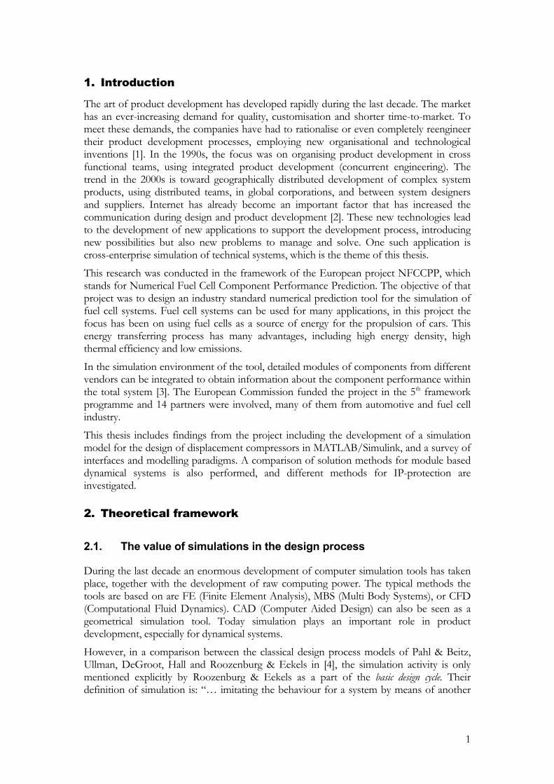
However, in a comparison between the classical design process models of Pahl & Beitz, Ullman, DeGroot, Hall and Roozenburg & Eekels in [4], the simulation activity is only mentioned explicitly by Roozenburg & Eekels as a part of the basic design cycle. Their definition of simulation is: “… imitating the behaviour for a system by means of another

2

system, which resembles the first system in certain respects, and therefore is a model of that first system” [5] .

Figure 1: The basic design cycle [5]

Even though simulations are not explicitly mentioned in these references, it does not mean that they should not be used in design. In a phase model, as defined by Pahl & Beitz [6], simulations can be used during the conceptual design, embodiment design and detail design. For example, in the concept phase, the system layout of fuel cell systems can be investigated using the models derived in this paper. In embodiment and detailed design, more sophisticated models can be developed to predict the performance of components. Even in the first phase, “clarifying the task”, simulation can be useful to give information, as to whether the product has any commercial potential and is worth developing.

Analysis

Function

Synthesis

Criteria

Simulation

Provisional design

Evaluation

Expected properties

Value of the design

Decision

Approved design

3

With the increasing availability of computing power and development of software, along with the higher complexity and customer demands on products, it is probable that simulation based design will be more efficient and play a larger role in future product development. In Sweden, national research programmes on simulation based design have been carried out during the last years, see for example ENDREA [7] or VISP [8].

2.2. Lumped modelling/discretisation

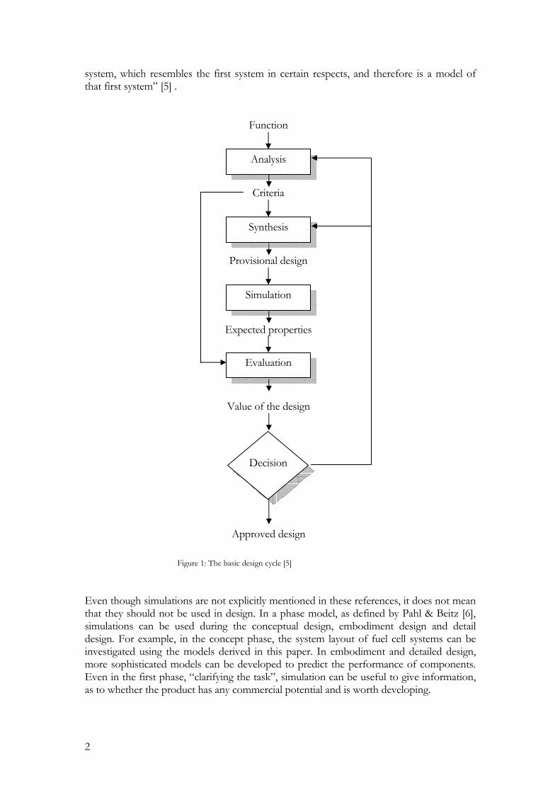
General engineering problems are often time dependent, non-linear, dependent on spatial coordinates, and thus mathematically described using non-linear partial differential equations (PDE:s) having time dependent coefficients/input. Since these equations are not directly solvable, and raw computing power is not an infinite resource, simplifications have to be made to get a numerically solvable and manageable system. Common simulation techniques are shown in Table 1:

FEM – dynamical

CFD – non-stationary

cont

inuo

us fi

eld

prob

lem

FEM – static

CFD – stationary

FEM – quasi-static

CFD – quasi-static

Lumped modelling

Rigid bodies

MBS SP

AC

E

disc

rete

Analytic formulas

Elementary cases

Function blocks

Stochastic processes

Event based process simulation

Function blocks Dynamical transfer functions

static discrete continuous

T I M E Table 1: Simulation techniques. The model complexity and computational effort are increasing from the lower left to the upper right corner. FEM – Finite Element Method, CFD – Computational Fluid Dynamics, MBS – Multi Body System [2]

A rule of thumb is that the simplest models are at the left bottom of the table, and the most advanced and most computationally expensive ones in the upper right corner of the table. In this work, the techniques lumped modelling and discretisation will be used. Lumped modelling is defined in [9]:

Lumped processes are all processes in which the spatial dependence of the variables under consideration can be neglected, i.e. in which a change in those variables is considered equal and simultaneous throughout the volume for which the laws of conservation have been established.

Discretisation can be defined as “the process of transferring continuous models and equations into discrete counterparts”, and is usually carried out as a first step toward making them suitable for numerical evaluation on digital computers [10]. PDE:s can be discretised in either time or space (or both), using differencing schemes. Discretisation in space is closely related to lumped modelling, as shown in the following example: If five one

4

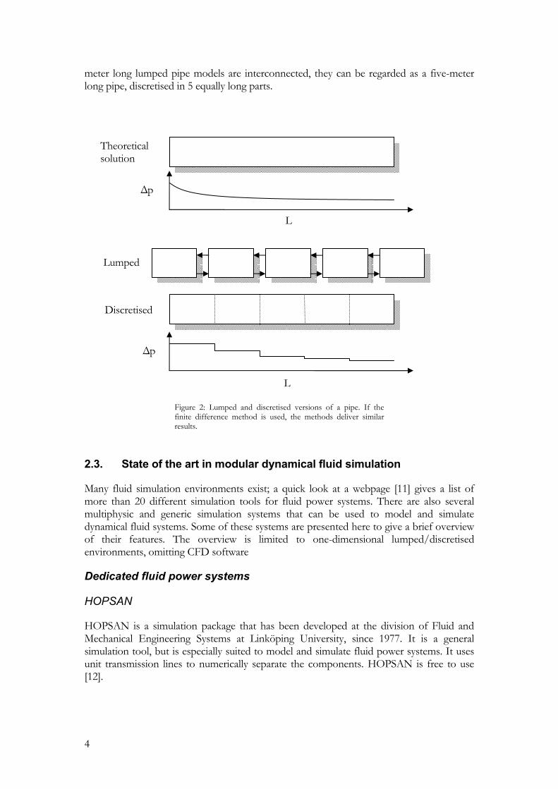
meter long lumped pipe models are interconnected, they can be regarded as a five-meter long pipe, discretised in 5 equally long parts.

Figure 2: Lumped and discretised versions of a pipe. If the finite difference method is used, the methods deliver similar results.

2.3. State of the art in modular dynamical fluid simulation

Many fluid simulation environments exist; a quick look at a webpage [11] gives a list of more than 20 different simulation tools for fluid power systems. There are also several multiphysic and generic simulation systems that can be used to model and simulate dynamical fluid systems. Some of these systems are presented here to give a brief overview of their features. The overview is limited to one-dimensional lumped/discretised environments, omitting CFD software

Dedicated fluid power systems

HOPSAN

HOPSAN is a simulation package that has been developed at the division of Fluid and Mechanical Engineering Systems at Linköping University, since 1977. It is a general simulation tool, but is especially suited to model and simulate fluid power systems. It uses unit transmission lines to numerically separate the components. HOPSAN is free to use [12].

∆p

L

L

∆p

Theoretical solution

Lumped

Discretised

5

Flowmaster

Flowmaster is according to its authors the “leading 1D thermofluid flow software package”. It was originally designed to simulate the fluid dynamical effects of fast acting pressure transients in complex networks. It includes component models for many generic fluid components such as pipes, valves and compressors. Flowmaster can be connected with other simulation tools, such as MATLAB/Simulink [13].

Multiphysic simulation systems

Easy5

Easy5 is a “schematic (iconic blocks) -based virtual product development software used to model, simulate, and analyse multidomain dynamic systems” [14]. The application libraries include gas dynamics, powertrains, electrical systems, multiphase fluids and even fuel cells. Easy5 also provides interfaces to numerous other simulation software including MATLAB/Simulink and MSC Adams.

AMESim

AMESim is “a complete 1D virtual system analysis platform that allows users to design multi-domain systems” [15]. The additional programs AMESet, AMECustom and AMERun are used to further extend the functionality. The program uses something they call multiport connections between components.

ITI-Sim

ITI-Sim is like AMESim a power-port simulation software for simulation of “dynamically stressed, complex non-linear systems”. It is also a commercial program, and 300 licences have been installed worldwide. It is developed by the German company ITI [16].

Modelica

Modelica is not a simulation environment, but a “free object-oriented modelling language with a textual definition to describe physical systems in a convenient way by differential, algebraic and discrete equations” [17]. There are however different solvers and graphical user interfaces that uses the Modelica language, such as the commercial Dymola or MathModelica. Modelica is a way of describing the environment and the governing equations. One of the main ideas behind Modelica is to describe the equations in a non-casual way and leave it to the solver to sort out the solution methods. In [18], it is for instance described how Modelica systems can be converted to and simulated in HOPSAN.

Generic simulation software

MATLAB/Simulink

MATLAB/Simulink is the leading software for technical computing and Model-Based Design. Simulink, which is bundled with MATLAB is a block model software, applied to model, simulate and analyse dynamical systems. It is widely used in control theory and digital signal processing for multidomain simulation and design. There exist many toolboxes for Simulink, but none for simulation of fluid systems, however [19].

6

VisSim

VisSim is another tool for simulating dynamical systems. It is a block model software, having signal ports. It is comparable with Simulink as it uses casual modelling. No specialised fluid library is currently available [20].

2.4. Model components and interfaces

A modular simulation environment includes components that are assembled to build a system simulation model. These component models represent mathematical models of the actual component. When interconnecting the components, well-defined interfaces are needed. The word interface can have many different meanings depending on the context. Here it is defined as “the means by which interaction and communication is achieved at the boundary between software components”. The interaction and communication of the physical parameters is of interest. It is desirable to have an interface having the same properties as the physical interface.

In literature, two paradigms exist: signal flow and power-port [21] (also known as signal port and multiport [22]). Signal flow has the background from analogue simulation environments, where the signal path is unidirectional. In block model software, such as MATLAB/Simulink or VisSim, all the inputs are on one side (usually the left), and all the outputs on the other side. It is even suggested that the main direction of the flow should be from left to right [23]. The signals are not differentiated to show differences between physical (effort and flow) and control signals. Using so-called power-ports is another solution, where effort and flow variables are used, one in each direction. The name power-port is given because of the fact that the product of the effort and flow has the dimension power.

Basically, power-ports can be regarded as signal ports, but adding a physical dimension, since both the effort and flow signals are at the same location in the model as in the physical object. To find out which variables to be used as input and as output in the power-port or signal port, the bond-graph method can be used. The bond-graph method is a method to find a proper solution order, especially for time dependent equations, where it is numerically preferred to integrate the equations than to differentiate them. The two main reasons behind this are that the derivative can go to infinity if a step input is applied, and that most difference schemes for the derivative are dependent on future values of the parameters. The bond-graph approach is valid for systems in different physical domains; the basic idea is to describe the system in terms of 9 basic elements. There are different rules as to how the basic elements should be interconnected.

Table 2: Physical analogies used in bond-graph modelling [24]

Another way is to have non-causal interfaces between the components, and to let the software decide on how to manage the calculations. Control signals can nevertheless have a specified direction. The topology of the system is thus preserved. Modelica is an example

Effort Flow Inertance Capacitance Resistance

Electricity Voltage Current Inductor Capacitor Resistor

Mechanics Force Velocity Mass Spring Friction

Flow Pressure Flow Pipe Volume (compressibility)

Friction

7

of this, where only the connections and how they are related are displayed, and separated from the solution process [25]. A “basic element approach” is also mentioned in [22], and it has also been implemented in AMESim.

Example application, a controlled valve

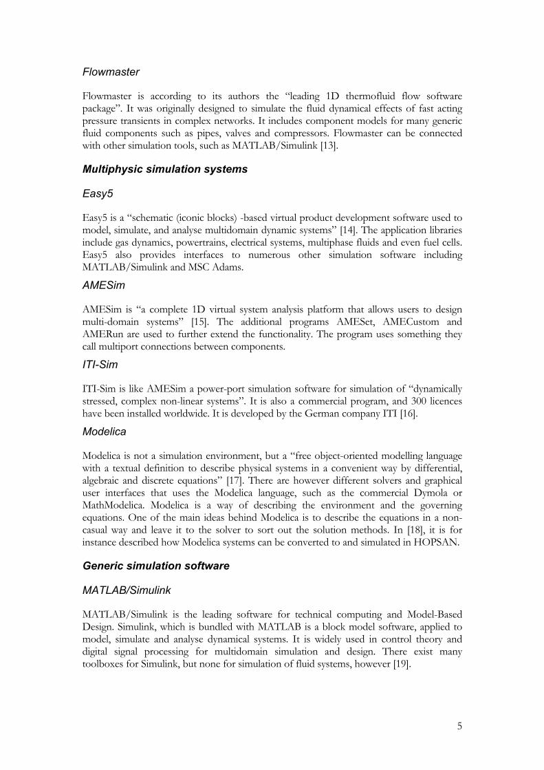
Figure 3: A simplified scheme for the component. This is similar to how the system appears in for example Modelica, Flowmaster or Easy5. BC stands for boundary condition.

To show the differences between these approaches, a small example has been prepared to illustrate this. The application is a three-way valve which controls the flow between the two branches: Branch 1 and Branch 2. The boundary conditions are given by a flow rate at one side, and a pressure level on the other side. Note that the boundary condition does not have to be a fixed value; it can be a time dependent function. Typically one wants to study the total pressure drop over the system, or determine what flow rates are achieved in the different branches.

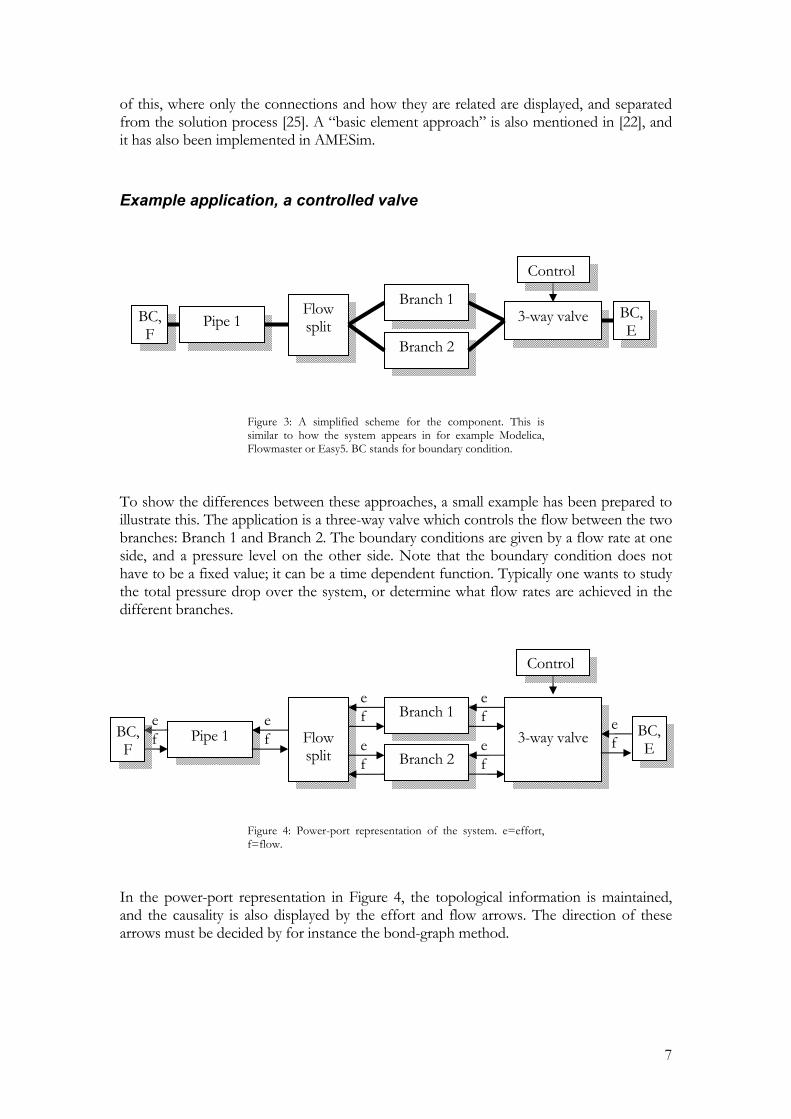
Figure 4: Power-port representation of the system. e=effort, f=flow.

In the power-port representation in Figure 4, the topological information is maintained, and the causality is also displayed by the effort and flow arrows. The direction of these arrows must be decided by for instance the bond-graph method.

Branch 1 3-way valve Flow

split Branch 2

Pipe 1

Control

BC, F

BC, E

Branch 1

3-way valve

Flow split Branch 2

Pipe 1 f e

f e

f e

f e

f e

f ef

e

Control

BC, E

BC, F

8

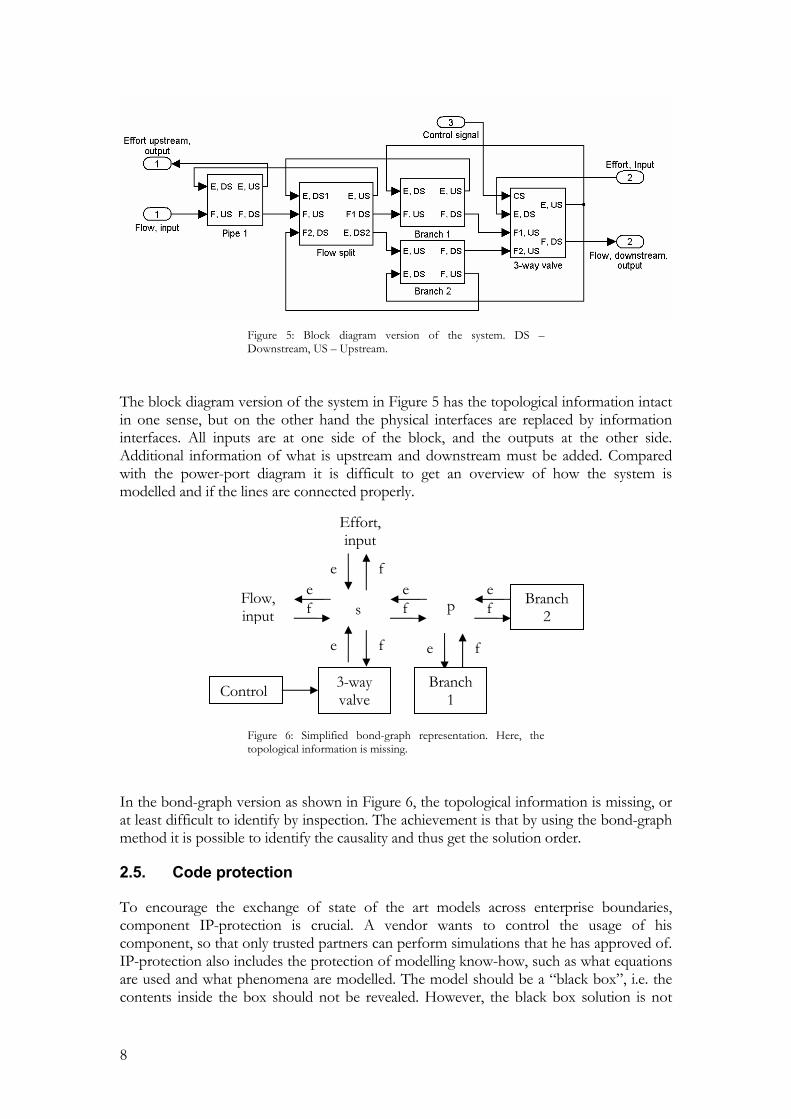
Figure 5: Block diagram version of the system. DS – Downstream, US – Upstream.

The block diagram version of the system in Figure 5 has the topological information intact in one sense, but on the other hand the physical interfaces are replaced by information interfaces. All inputs are at one side of the block, and the outputs at the other side. Additional information of what is upstream and downstream must be added. Compared with the power-port diagram it is difficult to get an overview of how the system is modelled and if the lines are connected properly.

Figure 6: Simplified bond-graph representation. Here, the topological information is missing.

In the bond-graph version as shown in Figure 6, the topological information is missing, or at least difficult to identify by inspection. The achievement is that by using the bond-graph method it is possible to identify the causality and thus get the solution order.

2.5. Code protection

To encourage the exchange of state of the art models across enterprise boundaries, component IP-protection is crucial. A vendor wants to control the usage of his component, so that only trusted partners can perform simulations that he has approved of. IP-protection also includes the protection of modelling know-how, such as what equations are used and what phenomena are modelled. The model should be a “black box”, i.e. the contents inside the box should not be revealed. However, the black box solution is not

Flow, input

p

Effort, input

e f

f e

s

e f

e f

f e

f e

3-way valve

Branch 1

Branch 2

Control

9

completely safe either. If the output and the input are recorded from the black box the parameters could be identified inside the box which is here referred to as clamping. When the black box only has non-dynamical relations, it is easy to get a map of the output. In dynamical systems, it is more difficult since the output is dependent on both the input and the time, but still feasible.

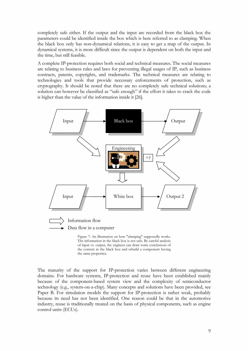
A complete IP-protection requires both social and technical measures. The social measures are relating to business rules and laws for preventing illegal usages of IP, such as business contracts, patents, copyrights, and trademarks. The technical measures are relating to technologies and tools that provide necessary enforcements of protection, such as cryptography. It should be noted that there are no completely safe technical solutions; a solution can however be classified as “safe enough” if the effort it takes to crack the code is higher than the value of the information inside it [26].

Figure 7: An illustration on how "clamping" supposedly works. The information in the black box is not safe. By careful analysis of input vs. output, the engineer can draw some conclusions of the content in the black box and rebuild a component having the same properties.

The maturity of the support for IP-protection varies between different engineering domains. For hardware systems, IP-protection and reuse have been established mainly because of the component-based system view and the complexity of semiconductor technology (e.g., system-on-a-chip). Many concepts and solutions have been provided, see Paper B. For simulation models the support for IP-protection is rather weak, probably because its need has not been identified. One reason could be that in the automotive industry, reuse is traditionally treated on the basis of physical components, such as engine control units (ECUs).

Black box

Engineering

Input

Output

White box

Output 2

=?

Input

Information flow Data flow in a computer

10

3. Research approach

The main objective behind this research was to find new methods to increase the efficiency and usability of simulation software for component manufacturers. In particular SME:s (Small and Medium-sized Enterprises) are targeted, since they do not have the resources or know-how to build a complete simulation system by themselves. The research approach has been to contribute to the NFCCPP-project as a member and continuously evaluate the approach against other scientific projects, commercial software and customer demands. During the work, research questions have been formulated in order to research special topics:

• How can a component-based modular simulation environment for fuel cells be created using block model software?

• What are the advantages and disadvantages of different approaches to modular modelling and different solution strategies?

• How can the intellectual property of a component be protected?

• How can general lumped models for transient flow in ducts and filling/emptying of volumes be formulated to be used in block model software?

4. Results

4.1. NFCCPP simulation model – in overview

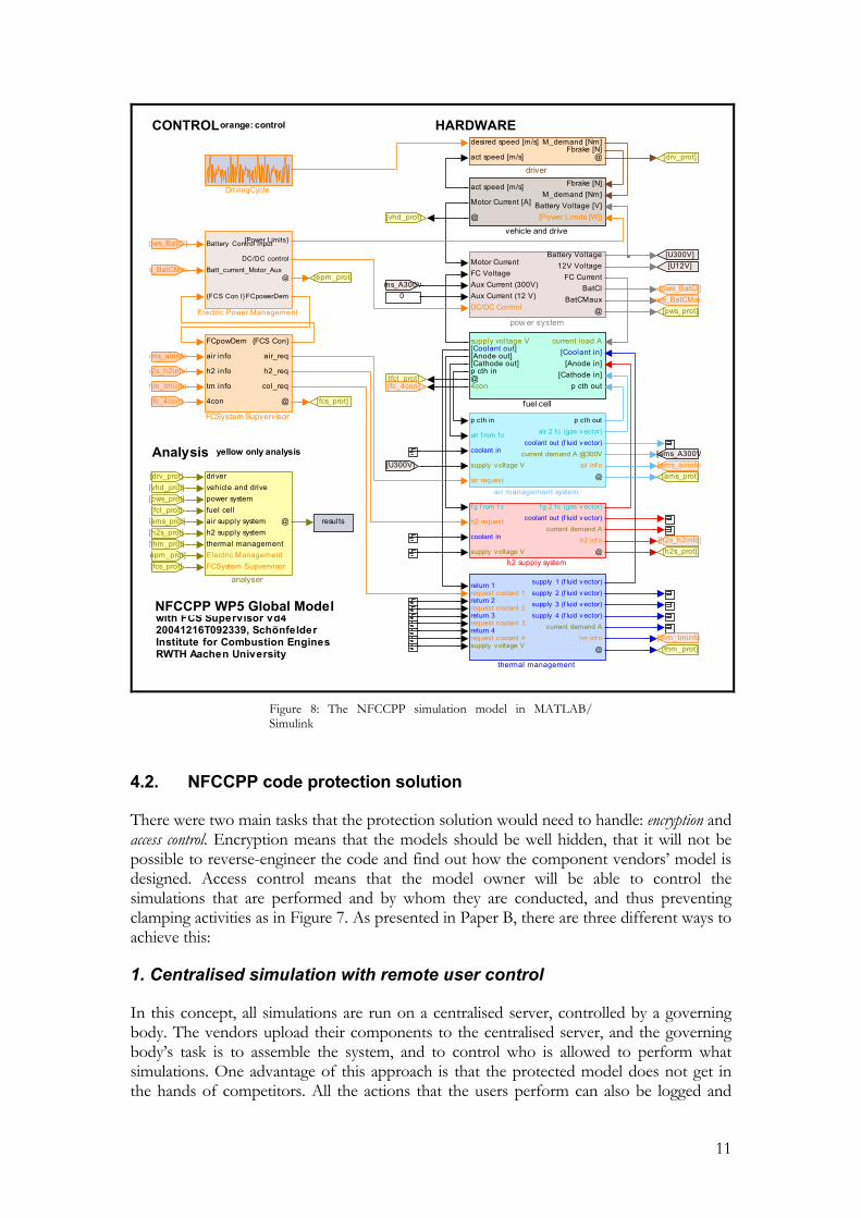
In the NFCCPP project, MATLAB/Simulink was chosen as the simulation environment. The reason for this was mainly that it is an industry standard tool that many project members were familiar with, and that SME:s probably have. It is also suitable for hardware-in-the-loop simulations, so that real components can be tested interacting with the software. MATLAB/Simulink also provides interfaces to many other simulation environments.

A complete system for a fuel cell in a prime mover was modelled, including air management system, hydrogen supply from an on-board gasoline reformer, drive train, driver and a control system. The system was simulated over the new European drive cycle [27] which is 1220 seconds and the model runs in about real-time on a standard desktop computer.

11

with FCS Supervisor vd4 20041216T092339, Schönfelder Institute for Combustion EnginesRWTH Aachen University

NFCCPP WP5 Global Model

CONTROL HARDWARE

Analysis

orange: control

yellow only analysis

Fbrake [N]M_demand [Nm]

Battery Voltage [V]{Power Limits [W]}

act speed [m/s]

Motor Current [A]

@

vehicle and drive

return 1request coolant 1return 2request coolant 2return 3request coolant 3return 4request coolant 4supply v oltage V

supply 1 (f luid v ector)

supply 2 (f luid v ector)supply 3 (f luid v ector)

supply 4 (f luid v ector)

current demand Atm inf o

@

thermal management

Motor CurrentFC VoltageAux Current (300V)Aux Current (12 V)DC/DC Control

Battery Voltage12V Voltage

FC CurrentBatCI

BatCMaux@

pow er system

f g f rom f c

h2 request

coolant in

supply v oltage V

f g 2 f c (gas v ector)

coolant out (f luid v ector)current demand A

h2 inf o

@h2 supply system

current load A[Coolant in]

[Anode in][Cathode in]

p cth out

supply voltage V[Coolant out][Anode out][Cathode out]p cth in@4con

fuel cell

desired speed [m/s]

act speed [m/s]

M_demand [Nm]Fbrake [N]

@

driver

drivervehicle and drive power system fuel cell air supply system h2 supply system thermal management Electric ManagementFCSystem Supvervisor

@

analyser

p cth in

air f rom f c

coolant in

supply v oltage V

air request

p cth out

air 2 f c (gas v ector)

coolant out (f luid v ector)

current demand A @300Vair inf o

@

air management system

results

[fcl_prot]

[pws_prot]

[vhd_prot]

[drv_prot]

[thm_tminfo]

[h2s_h2info]

[ams_airinfo

[U300V]

[fc_4con]

pws_BatCMau

[fcs_prot]

[epm_prot][pws_BatCI]

[thm_prot]

[h2s_prot]

[ams_prot]

[ams_A300V

[U12V]

[h2s_prot][ams_prot][fcl_prot]

[pws_prot][vhd_prot][drv_prot]

h2s_h2info]

ams_airinfo

[fc_4con]

s_BatCMau

pws_BatCI]

hm_tminfo]

epm_prot][fcs_prot]

[thm_prot]

ms_A300V

[U300V]

FCpowDem

air info

h2 info

tm info

4con

{FCS Con}

air_req

h2_req

col_req

@

FCSystem Supvervisor

Battery Control Input

Batt_current_Motor_Aux

{FCS Con I}

{Power Limits}

DC/DC control

@

FCpowerDem

Electric Power Management

DrivingCycle

0

Figure 8: The NFCCPP simulation model in MATLAB/ Simulink

4.2. NFCCPP code protection solution

There were two main tasks that the protection solution would need to handle: encryption and access control. Encryption means that the models should be well hidden, that it will not be possible to reverse-engineer the code and find out how the component vendors’ model is designed. Access control means that the model owner will be able to control the simulations that are performed and by whom they are conducted, and thus preventing clamping activities as in Figure 7. As presented in Paper B, there are three different ways to achieve this:

1. Centralised simulation with remote user control

In this concept, all simulations are run on a centralised server, controlled by a governing body. The vendors upload their components to the centralised server, and the governing body’s task is to assemble the system, and to control who is allowed to perform what simulations. One advantage of this approach is that the protected model does not get in the hands of competitors. All the actions that the users perform can also be logged and

12

monitored in many different ways, so as long as the vendors can trust the governing body they should feel safe using this solution.

2. Localised simulation with simulation-time model usage control

Here, the simulations are performed locally on the user’s computer, so the vendors need to supply protected components. To encrypt the components they are compiled, but reverse-engineering using methods such as disassembling can still be a risk. To satisfy the access control criteria, the surrounding simulation environment must be verified, to make sure that it has the configuration that the component manufacturer has allowed usage for. If the configuration is satisfactory, the model unlocks itself and the simulation can be run.

3. Parallel distributed simulation

Using distributed simulation, the simulation is run on many computers at the same time. Thus, the component models can stay at the vendors’ sites and use communication over the Internet to synchronise the simulations. Using this approach, there will be no need for encryption since the models never will leave the vendors’ site. This is the major feature of this concept. The drawback is that the communication must take place at a fast speed requiring high bandwidth and low latency, and must be compatible with IT-solutions such as firewalls. In addition, a framework on how to set up a system configuration and how it is checked needs to be developed.

Selected concept

Alternative 2, localised simulation with simulation-time model usage control, was decided to be further developed in the NFCCPP-project. The main reason for this was the ability to implement it in the framework of the project with respect to time and use efficiency. It is also the concept which has least impact on the end user, and that it also easily allows exchange of models on a bi-lateral basis without the need of a governing body.

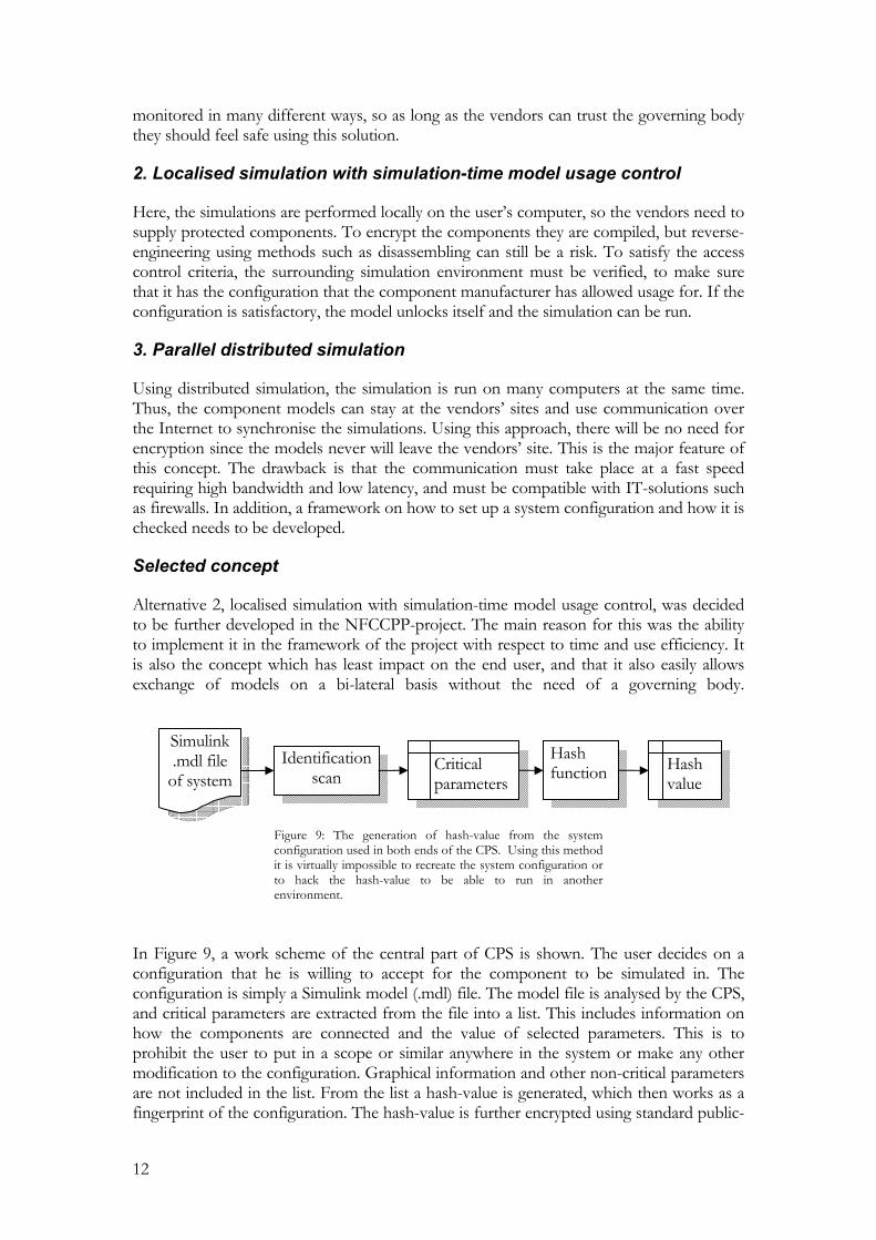
Figure 9: The generation of hash-value from the system configuration used in both ends of the CPS. Using this method it is virtually impossible to recreate the system configuration or to hack the hash-value to be able to run in another environment.

In Figure 9, a work scheme of the central part of CPS is shown. The user decides on a configuration that he is willing to accept for the component to be simulated in. The configuration is simply a Simulink model (.mdl) file. The model file is analysed by the CPS, and critical parameters are extracted from the file into a list. This includes information on how the components are connected and the value of selected parameters. This is to prohibit the user to put in a scope or similar anywhere in the system or make any other modification to the configuration. Graphical information and other non-critical parameters are not included in the list. From the list a hash-value is generated, which then works as a fingerprint of the configuration. The hash-value is further encrypted using standard public-

Simulink .mdl file

of system Identification

scan Hash function Critical

parameters Hash value

13

key encryption and then assembled with the code from the open component model and the CPS, to make a protected model. The protected model is compiled, and the binary code is also obfuscated in order to protect the code against reverse-engineering efforts. At runtime the embedded CPS in the protected model checks the .mdl file it is assembled in, and then creates a hash-value using the method described above. If the hash-values agree, the code will be decrypted and enabled.

Figure 10: A conceptual scheme of the architecture of the code protection system in UML syntax. The diamonds represent composition relationship, and the lines represent associative relations.

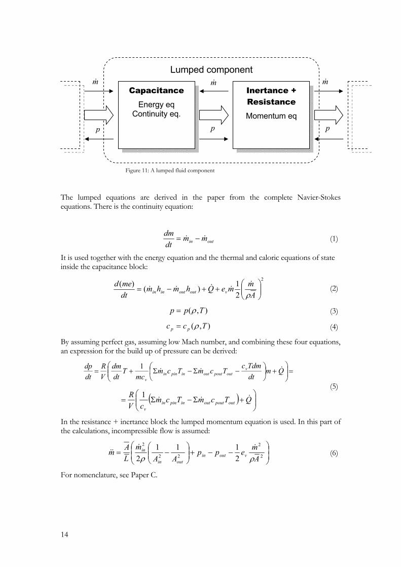
4.3. Governing equations

In Paper C, governing equations for a lumped fluid control volume are derived. In this derivation, assumptions and simplifications are documented. The equations are derived to fit in block model software (e.g. MATLAB/Simulink). The perfect gas law is assumed to be valid inside the control volume, and the flow is assumed to be completely in gas form, i.e. no two-phase flow is accounted for. The control volume is separated in two parts: a capacitance and a combined inertance + resistance block.

Open Component

Model

Server Software

Cryptography Facility

Client Software

Compilation Facility

Code Obfuscation

Facility

Protected Component

Model

Protection Mechanisms

Protection Software

Code Protection System

Control Key

Algorithms

Uses Produces

Implements

CompilesBinary encryption

14

Figure 11: A lumped fluid component

The lumped equations are derived in the paper from the complete Navier-Stokes equations. There is the continuity equation:

outin mmdtdm

&& −= (1)

It is used together with the energy equation and the thermal and caloric equations of state inside the capacitance block:

2

21)()(

++−=

AmmeQhmhm

dtmed

voutoutinin ρ&

&&&& (2)

),( Tpp ρ= (3)

),( Tcc pp ρ= (4)

By assuming perfect gas, assuming low Mach number, and combining these four equations, an expression for the build up of pressure can be derived:

=

+

−Σ−Σ+= QmdtTdmc

TcmTcmmc

Tdtdm

VR

dtdp v

outpoutoutinpininv

&&&1

( )

+Σ−Σ= QTcmTcm

cVR

outpoutoutinpininv

&&&1

(5)

In the resistance + inertance block the lumped momentum equation is used. In this part of the calculations, incompressible flow is assumed:

−−+

−= 2

2

22

2

2111

2 Amepp

AAm

LAm voutin

outin

in

ρρ&&

&& (6)

For nomenclature, see Paper C.

Lumped component

Capacitance Energy eq

Continuity eq.

Inertance + Resistance Momentum eq

m& m& m&

ppp

15

4.4. Using dynamical equations to solve large systems

As mentioned in the last section, the component consists of a capacitance and a resistance + inertance block. This can be compared to Krus [21], who describes a component of a capacitance and resistance block (i.e. no inertance). If the inertance part of the calculation is skipped, then the equation (6) becomes:

02111

2 2

2

22

2

=−−+

−

Amepp

AAm

voutinoutin

in

ρρ&&

(7)

If lumped components are modelled as in Figure 11, using equation (7) (resistance) instead of equation (6), the resulting equations will be a system of differential-algebraic equations, instead of a system of differential equations. It can be shown that for differential-algebraic equations, the calculation effort is more than linearly dependent on the size of the system [21]. If the dynamics are modelled, using equation (6), a set of stiff differential equations is obtained instead, which also takes much effort to solve. The solution presented in Paper C is to add a virtual mass factor K, to reduce the stiffness of the differential equations.

−−+

−= 2

2

22

2

2111

2 Amepp

AAm

LKAm voutin

outin

in

ρρ&&

&& (8)

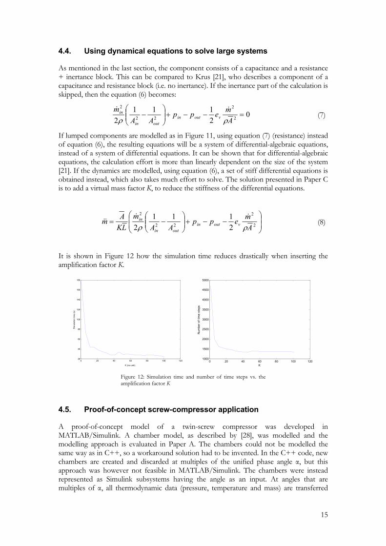
It is shown in Figure 12 how the simulation time reduces drastically when inserting the amplification factor K.

0 20 40 60 80 100 12020

40

60

80

100

120

140

160

180

K (no unit)

Sim

ulat

ion

time

(s)

0 20 40 60 80 100 1201000

1500

2000

2500

3000

3500

4000

4500

5000

Num

ber o

f tim

e st

eps

K Figure 12: Simulation time and number of time steps vs. the amplification factor K

4.5. Proof-of-concept screw-compressor application

A proof-of-concept model of a twin-screw compressor was developed in MATLAB/Simulink. A chamber model, as described by [28], was modelled and the modelling approach is evaluated in Paper A. The chambers could not be modelled the same way as in C++, so a workaround solution had to be invented. In the C++ code, new chambers are created and discarded at multiples of the unified phase angle α, but this approach was however not feasible in MATLAB/Simulink. The chambers were instead represented as Simulink subsystems having the angle as an input. At angles that are multiples of α, all thermodynamic data (pressure, temperature and mass) are transferred

16

one subsystem ahead. In practice, this is used by applying the MOD-function on the rotational angle to create a saw tooth like function with periodicity α. MOD is the standard mathematical modulus function. This signal triggers the external reset of the integration blocks, and the integration starts over, with external initial conditions from the preceding blocks. The phase angle is phase shifted α, 2α, 3α etc. up to the minimum number of chambers and used as input to the following block.

5. Discussion and conclusions

Since the result section is divided in different subjects, this discussion and conclusion section is also divided into these topics.

5.1. NFCCPP

The NFCCPP fuel cell system simulation model has been created, and it is unique since it is a component-based simulation environment that many major partners in the automotive industry have been involved in developing. This means that it serves its purpose of making an industry standard tool, at least for the involved companies. One of the main challenges is now how to disseminate the results to the rest of the industry (not involved in NFCCPP), and also how to maintain the software in the future. At the time of writing this, strategies for these two tasks are being developed in the NFCCPP consortium. There are also other approaches for creating a standard simulation tool, see for example CAPSIM [29]. Many of the simulation environments mentioned in Section 2 are also claimed to work as a common modelling environment for cross-enterprise simulations.

5.2. Code protection

Three different approaches have been developed and evaluated. An implementation of the concept “Localised simulation with simulation-time model usage control” has been developed using MATLAB/Simulink within the NFCCPP-project. The most promising concept for future work is however “Parallel distributed simulation”, but many technical problems remain to be solved.

5.3. Different approaches to formulate and solve dynamical fluid equations

The advantage of describing the topology of the system using a scheme like in Figure 3 compared with the other descriptions is obvious; it is the one that resembles the actual physical system. The block diagram version in Figure 5 is more difficult to follow, and this could depend on the fact that this approach is developed from the simulation on electronic analogue computers, a popular tool of system dynamics in the 1950-1970s [30]. In control engineering the block diagram model is useful, since the signals have a specified direction. But for physical modelling, where the direction of the signal is derived from a mathematical model of the system, it is not as useful. The signal port approach is however easier for the computer to interpret, since the causality is given, the computer only has to carry out the integration. No simulation software uses the power-port approach described in Figure 5 to combine the advantage of having a topological system together with being able to specify the causality. This would improve the readability of large simulation systems in block model software a lot, and it should be uncomplicated to implement.

17

Using a topological representation as in Figure 3, there are different ways the software can derive the underlying equations and causality. For some products like HOPSAN, it is documented how the interfaces work, but for other softwares it might be company secrets.

5.4. Using dynamical equations to solve the system

It has been shown that this method works, and that it can be implemented in MATLAB/Simulink. A more detailed mathematical analysis of this method could be made in order to make an estimation of the error, and finding proper values of the constant K. It can be seen in Figure 12 that the decrease in simulation time is flattened out when exceeding a limit value of K. Using this method, algebraic equations can be avoided, and thus a linear relationship between the number of components and the simulation time can be achieved, which is important in large simulation systems.

6. Synergy of the treated topics and contributions

In the introduction section, it is mentioned that the background is how to be able to perform cross-enterprise simulation of complex engineering systems. Paper A presents a typical detailed model of a system component. This model will however not be used directly in the system model, it would rather be used to generate a performance map. This is because of limited calculation time, and that it is simply not necessary to model all phenomena when determining the system performance. The performance map could also be generated from another software model, such as a CFD-model of a fuel cell stack or an MBS model of a car.

The NFCCPP model described in Paper B describes a cross-enterprise simulation system. To allow other companies to use the performance map, and to be able to release it, the need for code protection arises. Paper C describes the governing fluid equations and could therefore be used as a starting point when developing a simplified fluid component model to use in the system. To further reduce the simulation time, the virtual mass technique, also described in Paper C, can be employed. Some drawbacks by using block model software to model physical phenomena are explained in this summary, and other simulation environments are listed and presented in short. To use a causal simulation environment, the power-port representation is suggested to preserve the topological information.

18

7. Summary of appended papers

7.1. Paper A: Modelling of displacement compressors using MATLAB/Simulink

This paper gives a proof-of-concept model of a displacement compressor in MATLAB/Simulink. The modelling idea is based on the same idea as the state of the art one-dimensional displacement compressor simulation software [28], but adopted to the visual MATLAB/Simulink environment. It is described how moving geometries can be modelled in MATLAB/Simulink, and how to model geometries having variable volume in time.

7.2. Paper B: Virtual Component Testing for PEM Fuel Cell Systems

This paper was written by some members of the NFCCPP consortia, and describes the outcome of the project. The NFCCPP software is described, together with the methods used to model the software including interfaces, integration of the components and more. A more detailed description is given on how the fuel cell and the reformer path are modelled using a combined theoretical/empirical approach. The model protection, which could be the part with most news value in the NFCCPP project, is described in this paper.

7.3. Paper C: The design of modular dynamical fluid simulation systems

This paper has many achievements. Firstly the lumped fluid equations are derived from the complete Navier-Stokes equations. This is done to show where simplifications (i.e. modelling errors) are introduced, and to be used as a reference. Secondly, different techniques for simulating modular dynamical fluid systems are discussed. A way to describe a generic fluid component in a causal simulation system, such as MATLAB/Simulink, is described. Besides, a well-known trick to cut down simulation time dramatically is documented. The trick is to add “virtual mass” to the outputs and thus slow down the mass-acceleration. By increasing the time constant for this phenomenon, larger time-steps can be used. The modelling error will be in the time-domain, since the steady state solution will be the same.

8. Future work

In the code protection topic, it would be interesting to develop the “Parallel distributed simulation” concept further. This concept has the most potential, and it is linked to other research on distributed simulation and co-simulation. The concept “Localised simulation with simulation-time model usage control” could also be implemented in other software packages such as Modelica or VisSim.

The virtual mass technique should be investigated more carefully, and be analysed more thoroughly. The error in the time domain should also be estimated. The block containing the differential equations could maybe be separated, and this method could thus be used as a generic tool to break algebraic loops, like transfer functions work today. Maybe this technique could be used in three dimensions as well.

19

Regarding the screw compressor model, a model at this level of detail is not of interest for system simulation. The development of CFD-models of screw compressors has started to produce results, so this will probably be the future in computer modelling for screw compressor development [31], [32]. The CFD model can also be used to generate a map to use in a system simulation environment.

9. References

[1] Hammer, M., Champy, J, Reengineering the Corporation: A Manifesto for Business Revolution, Harper Collins, New York, U.S.A., 1993

[2] Johannesson, H., Persson, J-G., Pettersson, D., Produktutveckling – effektiva metoder för konstruktion och design, Liber, Stockholm, Sweden, 2004

[3] NFCCPP Project poster, ENK5-CT-2002-00692, Cordis, Belgium, 2002

[4] Keski-Seppälä, S., Critical requirements on Computational Fluid Dynamics simulation within Engineering Design, Licentiate Thesis, Royal Institute of Technology, Stockholm, Sweden, 1999

[5] Roozenburg, N.F.M., Eekels, J., Product Design: Fundamentals and Methods, Wiley & Sons, Chichester, England, 1995

[6] Pahl, G., Beitz, W., Engineering Design – A Systematic Approach, Springer-Verlag, Berlin, Germany, 1999

[7] ENDREA homepage www.endrea.sunet.se, 2005-10-01

[8] VISP homepage, extra.ivf.se/visp/, 2005-10-01

[9] Kecman, V., State-Space Models of Lumped and Distributed Systems, Springer-Verlag, Berlin, Germany, 1988.

[10] Wikipedia, www.wikipedia.org, 2005-10-03

[11] Fluid Power Net homepage. fluid.power.net/fpn/wwwvl/docs/software.php3 2005-10-06

[12] HOPSAN homepage, hydra.ikp.liu.se/HOPSAN.html, 2005-10-06

[13] Flowmaster homepage, www.flowmaster.com, 2005-10-07

[14] MSC homepage, www.mscsoftware.com, 2005-10-12

[15] AMESim homepage, www.amesim.com, 2005-10-06

[16] ITI-Sim homepage, www.iti.de, 2005-10-06

[17] Modelica homepage, www.modelica.org, 2005-10-12

[18] Johansson, B., Krus, P., Modelica in a distributed environment using transmission line modelling, Modelica 2000 Workshop, Lund, Sweden, 2000

[19] The Mathworks homepage, www.themathworks.com, 2005-10-07

[20] VisSim homepage, www.vissim.com, 2005-10-10

[21] Krus, P., Modelling and Simulation of Heterogenous Engineering Systems, Linköping University, Linköping, Sweden, 2003

20

[22] Lebrun, M., Richards, C.W., How to create good models without writing a single line of code, International Fluid Power Congress SCIFP, Linköping, Sweden, 1997

[23] MAAB Style Guidelines, MathWorks Automotive Advisory Board, 2001

[24] Ljung, L., Glad, T., Modellbygge och simulering, Studentlitteratur, Lund, Sweden, 1991

[25] Modelica tutorial, version 1.4, Modelica Association, 2000

[26] Schneier, B., Applied Cryptography, second edition, John Wiley & Sons, New York, U.S.A., 1996

[27] Emission test cycles homepage, www.dieselnet.com/standards/cycles, 2005-10-22

[28] Kauder, K., Janicki, M., Rohe, A., Kliem, B., Temming, J., Thermodynamic Simulation of Rotary Displacement Machines”, VDI-Berichte 1715, Schraubenmaschinen 2002, pp 1-16

[29] CAPSIM homepage, www.capsim.se, 2005-11-01

[30] Doebelin, E. O., System Dynamics: Modeling, Analysis, Simulation, Design, Marcel Dekker Inc, New York, U.S.A., 1998

[31] Kovacevic, A., Stosic, N., Smith, I. K., CFD analysis of screw compressor performance, IMechE Symposium “Advances of CFD in Fluid Machinery Design”, London, England, 2001

[32] Elder, R., Tourlidakis, A., Yates, M., Advances of CFD in Fluid Machinery Design, Professional Engineering Publishing, Bury St Edmunds, England, 2003