
On the force-free magnetosphere of aligned rotator - arXiv · On the force-free magnetosphere of...
19
arXiv:astro-ph/0511817v2 13 Feb 2006 Mon. Not. R. Astron. Soc. 000, 1–19 () Printed 11 April 2018 (MN L A T E X style file v2.2) On the force-free magnetosphere of aligned rotator A. N. Timokhin ⋆ Sternberg Astronomical Institute, Universitetskij pr. 13, 119992 Mocsow, Russia Accepted Received ; in original form ABSTRACT We investigate in details properties of stationary force-free magnetosphere of aligned rotator assuming the last closed field line lying in equatorial plane at large distances from pulsar. The pulsar equations is solved numerically using multigrid code with high numerical resolution, physical properties of the magnetosphere are obtained with high accuracy. We found a set of solutions with different sizes of the closed magnetic field line zone and verify the applicability of the force-free approximation. We discuss the role of electron-positron cascades in supporting of the force-free magnetosphere and argue that the closed field line zone should grow with time slower than the light cylinder. This yield the pulsar breaking index less than 3. It is shown, that models of aligned rotator magnetosphere with widely accepted configuration of magnetic field, like one considered in this paper, have serious difficulties. We discuss solutions of this problem and argue that in any case pulsar energy losses should evolve with time differently than predicted by the magnetodipolar formula. Key words: stars:magnetic fields – pulsars:general – MHD 1 INTRODUCTION Since the first works on pulsar magnetosphere, a stationary force-free magnetosphere of aligned rotator is considered as an underlying model for the real pulsar magnetosphere for more than 30 years. Despite its degenerated character (such “pulsar” even does not pulse), it is believed to reproduce qualitatively all main properties of the real pulsar magne- tosphere. For near-aligned pulsars it should give even an adequate detailed description. The structure of aligned rota- tor’s force-free magnetosphere can be described by solution of a single scalar non-linear PDE, the so-called “pulsar equa- tion”, derived by Michel (1973b); Scharlemann & Wagoner (1973); Okamoto (1974). This is an equation for the flux of poloidal magnetic field. All other physical quantities describ- ing the magnetosphere are related to the flux function Ψ, poloidal current J and angular velocity of magnetosphere’s rotation Ω by algebraic relations. Analytical solution of this equation with non-zero poloidal current seems exist only for the split-monopole configuration of the magnetic field (Michel 1991) and for a slightly perturbed split monopole (Beskin et al. 1998). For dipole magnetic field analytical solution for the case of zero poloidal current has been found (Michel 1973a; Mestel & Wang 1979), but this solution is valid only inside the light cylinder (LC). There were several works dedicated to solution of linearised pulsar equation, where poloidal cur- rent and angular velocity were assumed to be proportional ⋆ E-mail: [email protected] to magnetic flux function, what made the equation linear, but they did not lead to construction of a consistent model of aligned rotator magnetosphere (see e.g. Beskin et al. 1983; Lyubarskii 1990; Beskin & Malyshkin 1998). The first attempt to solve this equation numerically was made by Contopoulos et al. (1999), hereafter CKF. They have shown for the first time, that there exists a self-consistent solution with dipole magnetic field geome- try near the NS and magnetic field lines smoothly pass- ing through the light cylinder. In that work the position of the null point 1 was fixed at the light cylinder and the question about applicability of the force-free approximation have been not investigated. Energy losses of the aligned ro- tator for CKF solution have been calculated by Gruzinov (2005). Goodwin et al. (2004) have studied this problem more deeply, namely they have searched for solution of the pulsar equation when the position of the null point is not fixed at the LC, but lies at different positions inside the light cylinder. For any position of the null point they obtained so- lutions, smoothly passing the light cylinder, but like CKF they have not studied physical properties of obtained solu- tions (e.g. energy losses, applicability of the force-free ap- proximations etc.). Their model, however, seems to be arti- ficial, because they assumed non-zero pressure in the closed field line zone, what implies continuous energy injection into the closed field line domain. Recently Contopoulos (2005) 1 the point where the last closed field line intersects the equatorial plane
Transcript of On the force-free magnetosphere of aligned rotator - arXiv · On the force-free magnetosphere of...

arX
iv:a
stro
-ph/
0511
817v
2 1
3 Fe
b 20
06
Mon. Not. R. Astron. Soc. 000, 1–19 () Printed 11 April 2018 (MN LATEX style file v2.2)
On the force-free magnetosphere of aligned rotator
A. N. Timokhin⋆
Sternberg Astronomical Institute, Universitetskij pr. 13, 119992 Mocsow, Russia
Accepted Received ; in original form
ABSTRACT
We investigate in details properties of stationary force-free magnetosphere of alignedrotator assuming the last closed field line lying in equatorial plane at large distancesfrom pulsar. The pulsar equations is solved numerically using multigrid code withhigh numerical resolution, physical properties of the magnetosphere are obtained withhigh accuracy. We found a set of solutions with different sizes of the closed magneticfield line zone and verify the applicability of the force-free approximation. We discussthe role of electron-positron cascades in supporting of the force-free magnetosphereand argue that the closed field line zone should grow with time slower than the lightcylinder. This yield the pulsar breaking index less than 3. It is shown, that models ofaligned rotator magnetosphere with widely accepted configuration of magnetic field,like one considered in this paper, have serious difficulties. We discuss solutions ofthis problem and argue that in any case pulsar energy losses should evolve with timedifferently than predicted by the magnetodipolar formula.
Key words: stars:magnetic fields – pulsars:general – MHD
1 INTRODUCTION
Since the first works on pulsar magnetosphere, a stationaryforce-free magnetosphere of aligned rotator is considered asan underlying model for the real pulsar magnetosphere formore than 30 years. Despite its degenerated character (such“pulsar” even does not pulse), it is believed to reproducequalitatively all main properties of the real pulsar magne-tosphere. For near-aligned pulsars it should give even anadequate detailed description. The structure of aligned rota-tor’s force-free magnetosphere can be described by solutionof a single scalar non-linear PDE, the so-called “pulsar equa-tion”, derived by Michel (1973b); Scharlemann & Wagoner(1973); Okamoto (1974). This is an equation for the flux ofpoloidal magnetic field. All other physical quantities describ-ing the magnetosphere are related to the flux function Ψ,poloidal current J and angular velocity of magnetosphere’srotation Ω by algebraic relations.
Analytical solution of this equation with non-zeropoloidal current seems exist only for the split-monopoleconfiguration of the magnetic field (Michel 1991) and fora slightly perturbed split monopole (Beskin et al. 1998).For dipole magnetic field analytical solution for the caseof zero poloidal current has been found (Michel 1973a;Mestel & Wang 1979), but this solution is valid only insidethe light cylinder (LC). There were several works dedicatedto solution of linearised pulsar equation, where poloidal cur-rent and angular velocity were assumed to be proportional
⋆ E-mail: [email protected]
to magnetic flux function, what made the equation linear,but they did not lead to construction of a consistent model ofaligned rotator magnetosphere (see e.g. Beskin et al. 1983;Lyubarskii 1990; Beskin & Malyshkin 1998).
The first attempt to solve this equation numericallywas made by Contopoulos et al. (1999), hereafter CKF.They have shown for the first time, that there exists aself-consistent solution with dipole magnetic field geome-try near the NS and magnetic field lines smoothly pass-ing through the light cylinder. In that work the positionof the null point1 was fixed at the light cylinder and thequestion about applicability of the force-free approximationhave been not investigated. Energy losses of the aligned ro-tator for CKF solution have been calculated by Gruzinov(2005). Goodwin et al. (2004) have studied this problemmore deeply, namely they have searched for solution of thepulsar equation when the position of the null point is notfixed at the LC, but lies at different positions inside the lightcylinder. For any position of the null point they obtained so-lutions, smoothly passing the light cylinder, but like CKFthey have not studied physical properties of obtained solu-tions (e.g. energy losses, applicability of the force-free ap-proximations etc.). Their model, however, seems to be arti-ficial, because they assumed non-zero pressure in the closedfield line zone, what implies continuous energy injection intothe closed field line domain. Recently Contopoulos (2005)
1 the point where the last closed field line intersects the equatorialplane
c© RAS

2 A. N. Timokhin
addressed the case when the plasma rotation frequency inthe open field line domain is different from the rotation fre-quency of the NS. It was shown, that there exist an uniquesolution of the pulsar equation for arbitrary plasma rotationfrequency, although a rather simple case when the plasmarotation frequency is constant have been considered. Ap-plicability of the force-free approximations in the magneto-sphere of aligned rotator was considered in Timokhin (2005)and Contopoulos (2005), though in the latter work only forthe null point located at the LC.
Recently a different approach to the pulsar magneto-sphere modelling is being developed by Spitkovsky (2005),Komissarov (2005), and McKinney (2006). They performtime-dependent simulations of the pulsar magnetosphere. InKomissarov (2005) aligned rotator magnetosphere was mod-elled using full MHD code, in McKinney (2006) the samemodelling was done with force-free code. The code of Ana-toly Spitkovsky allows performing of 3-D time-dependentsimulation of the magnetosphere of inclined rotator by solv-ing equations of force-free MHD. In these simulations theexistence of the stationary force-free magnetospheric config-uration was rigorously proved for the first time. Althoughthis approach presents a big step towards the modelling ofthe real pulsar magnetosphere, in this paper we argue thatit has serous limitation, namely the properties of cascadessupplying particles in magnetosphere are not incorporated inthese simulations. As it will be discussed later, cascades canset non-trivial boundary conditions on the current densityin the magnetosphere. Its incorporation in time-dependentcodes would require some efforts.
In this work we investigate stationary problem solvingthe pulsar equation numerically with high numerical resolu-tion. We assume zero pressure in the closed field line region(cold plasma). As in all above mentioned works on numer-ical modelling of stationary aligned rotator magnetospherewe assume a topology with the current sheet in open fieldline domain flowing in the equatorial plane, i.e. configurationwith Y null point – see Fig. 1. This type of magnetospheretopology had became de facto the “standard model”, so westudy it in details and analyse its properties regarding manyaspects of electrodynamics. Smooth solutions are obtainedfor any position of the null point inside the light cylinder.High numerical resolution allows accurately incorporationof the return current flowing along the separatrix into nu-merical procedure. With the high resolution of used numer-ical method it was possible to calculate accurately physicalproperties of the solutions such as Goldreich-Julian chargedensity, magnetic field, energy losses and pointing flux dis-tribution etc., check applicability of the force-free approxi-mation and consider compatibility of the model with modelsof electron-positron cascades.
Adjustment of the current density in the polar cap cas-cade zone of pulsar to the global magnetospheric structurewas debated already in the first ten years after pulsar dis-covery (see e.g. Arons 1979). A concrete mechanism for thecurrent density adjustment was proposed by Yu. Lyubarskijmany years later, in 1992. At that time there was no self-consistent model of pulsar magnetosphere and detailed dis-cussion on this subject was difficult. Here we discuss thecoupling between the polar cap cascade zone and the rest ofthe magnetosphere in the frame of the self-consistent modelobtained in our simulations. We extend the picture proposed
z
Ro
tati
on
Ax
is
Lig
ht
Cy
lind
er
separatrixx
open field lines
[2]
open field lines
[2′]
closed field lines
[1] Ireturn
I
b b
x0 1
A
Figure 1. Configuration of magnetic field in the magnetosphereof aligned rotator with Y null point – Y-configuration. After thenull point x0 the separatrix goes along the equatorial plane. Thevolume current I flowing in the open filed line zones [2] and [2′]closes somewhere beyond the light cylinder. There could be avolume return current along some open field lines, but the largestpart of it flows along the separatrix.
by Lyubarskij (1992) addressing the evolution of the cur-rent adjustment mechanism with ageing of the pulsar. Wealso prove the necessity of such mechanism and discuss itin more details in the frame of the cascade model proposedby Scharlemann et al. (1978). We underline serious difficul-ties of model with Y null point regarding its compatibilitywith the Space Charge Limited Flow models of polar capcascades and briefly discuss other possible magnetosphericconfiguration.
The plan of the paper is the following. In Section 2important properties of the pulsar equation are discussed.Model used in the current work and numerical method aredescribed in Section 3. Results of numerical simulations arepresented in Section 4. In section 5 we discuss the role ofpolar cap cascades for the global structure of the magneto-sphere, consider in details properties of the force-free mag-netosphere with Y null point, and highlight problems of the“standard” model of aligned rotator magnetosphere. A dif-ferent topology of the magnetosphere, with X null point, isbriefly discussed at the end of the section. We summarisethe most important results in Section 6.
2 THE PULSAR EQUATION
2.1 General equation
Here we adopt the wide used assumption, that the entire
magnetosphere of the neutron star (NS) is filled with plasma.In some works starved magnetosphere configuration havebeen debated (see e.g. Smith et al. 2001; Petri et al. 2002),where there are several separated clouds of charged parti-cles near the NS and no particle outflow, however thereare indications that such configuration is unstable againstdiocotron instability (Spitkovsky & Arons 2002; Spitkovsky2004). Plasma in the magnetosphere has to be non-neutral
c© RAS, MNRAS 000, 1–19

On the force-free magnetosphere of aligned rotator 3
in order to screen the longitudinal (directed along magneticfield lines) component of the electric field, induced by ro-tation of the NS. In presence of the longitudinal electricfield charged particles would be accelerated and their radia-tion will lead to copious electron-positron pair production insuper-strong magnetic field of pulsar (Sturrock 1971), whatfinally results in screening of the accelerating field.
Charge density necessary for cancelling of the longitudi-nal electric field, the so-called Goldreich-Julian (GJ) chargedensity (Goldreich & Julian 1969), near the neutron star isgiven by
ρGJ ≃ −Ω ·B2πc
, (1)
where Ω is angular velocity on neutron star rotation, B ismagnetic field and c is the speed of light. Assuming that NShas dipolar magnetic field, the ratio of the particle kineticenergy density in the magnetosphere to the energy densityof the magnetic field at the distance r can be estimated as
εkinεB
∼ (ρGJ/e) mec2γ
(B2/8π)≃
≃ 1.4× 10⁻¹¹P−1(
γ
107
)(
B0
1012 G
)−1 ( r
RNS
)3
,
(2)
where e and me are electron charge and mass correspond-ingly, RNS – neutron star radius, γ – Lorentz factor of accel-erated particles, B0 magnetic field strength in Gauss nearmagnetic poles of the star and P – period of pulsar rotationin seconds. All these quantities are normalised to their typi-cal values in pulsars. This ratio is small, less than 1 per cent,in the region with the size ∼ 103 P−1 radii of the neutronstar. It could remain small even further, but here magneticfiled deviates substantially from the NS’s dipole field due tocurrents flowing in the magnetosphere, and εkin/εB can beestimated only after a self-consistent solution for the magne-tosphere structure is found. So, in a large domain surround-ing the neutron star, we can use force-free approximation,when particle inertia is neglected, and equation of motiontakes the form
ρE +1
c[j×B] = 0. (3)
Hence, electric field E is perpendicular to the magnetic fieldB. Charge density ρ and current density j in eq. (3) can befound from the Maxwell equations (we consider stationaryproblem)
∇ ·E = 4πρ , (4)
∇×B =4π
cj , (5)
With help of these equations equation (3) can be written as
(∇ ·E) E + [∇×B]×B = 0 . (6)
In the force-free electrodynamics (FFE)2 the only possiblemotion of charged particles across magnetic field lines is thedrift in crossed electrical and magnetic fields with the veloc-ity
UD = cE×B
B2. (7)
2 hereafter we use this shorter name for force-free degenerateelectrodynamics (see e.g. Komissarov 2002; Blandford 2002, andreferences there)
Obviously |UD| must be less than c, or equivalently E mustbe less than B. Generally speaking, eq. (3) can have solu-tions where |UD| > c. The surface, where |UD| reaches c,is commonly referred as the light surface. Beyond the lightsurface, where |UD| > c, the force-free approximation cannot be applied. FFE is not self-consistent, because particledynamics is ignored. Hence, each solution of eq. (6) shouldbe always checked for applicability of the force free approx-imation.
In the axisymmetric stationary case considered heremagnetic field in cylindrical coordinates (,φ,Z) can bewritten as
B =∇Ψ× eφ
+
4π
c
I
eφ , (8)
where eφ is the unit azimuthal, toroidal vector. In compo-nents
(B, Bφ, BZ) = (− 1
∂ZΨ,
4π
c
I
,
1
∂Ψ) . (9)
Scalar function Ψ is related to the magnetic flux Φmag troughthe circle with the centre at the point (0, Z) and radius by Φmag = 2πΨ(,Z). So, lines of constant Ψ coincideswith magnetic field lines. It could be easily verified, that inforce-free case the scalar function I(,Z) is constant alongmagnetic field lines, i.e
I ≡ I(Ψ) . (10)
I is related to the total current J outflowing trough theabove mentioned circle by J = 2πI(,Z).
In the quasi-stationary case the time derivative of Btakes the form (see Mestel 1973)
∂B
∂t= ∇×([Ω×r]×B) . (11)
Substituting this into the Faraday’s law
∇×E = −1
c∂tB , (12)
we get for the electric field
E = −Ω×r
c×B −∇V = −Ω
c∇Ψ−∇V , (13)
where V is the non-corotational (see below) part of elec-tric potential. The first term in (13) is poloidal and onlythe second term could make a contribution to the toroidalcomponent. In axisymmetric case ∂φV = 0 and, hence, Eis poloidal. In the force-free case E ⊥ B, from this followsthat E · (∇Ψ×eφ) = 0. Consequently, E ∝ ∇Ψ and we canwrite
E = −ΩF
c∇Ψ , (14)
or in components
(E, Eφ, EZ) = (−ΩF
c∂Ψ, 0, −
ΩF
c∂ZΨ) . (15)
Substituting this expression together with eq. (8) into theformula for the drift velocity (7), we get
UD = ΩFeφ − 4π
c
IΩF
B2B ≡ ΩF×r − κB . (16)
So, the particle motions is composed from rotation with theangular velocity ΩF and gliding along magnetic field lines.
c© RAS, MNRAS 000, 1–19

4 A. N. Timokhin
Hence, ΩF is the angular velocity of magnetic field lines ro-tation. By substitution of eq.(14) into the stationary Fara-day’s law one find ∇ΩF×∇Ψ = 0. This implies that ΩF isconstant along magnetic field lines:
ΩF ≡ ΩF(Ψ) . (17)
Equation (17) is the well known Ferraro isorotation law.Finally, substituting E and B from eqs. (8), (14) into
equation (6) we get(
1− Ω2F
2
c2
)
∇2Ψ− 2
∂Ψ+
+(
4π
c
)2
IdI
dΨ− 2
c2ΩF
dΩF
dΨ(∇Ψ)2 = 0 (18)
This is Grad-Shafranov equation for the poloidal mag-netic field, the so-called pulsar equation, derived by Michel(1973b); Scharlemann & Wagoner (1973); Okamoto (1974).This scalar PDE is of elliptical type. It is the poloidal partof the vector equation (6). The toroidal part of eq. (6) issimply the relation (10). Pulsar equation has two integralsof motion – I and ΩF. If we know them, we can solve thisequation for function Ψ and determine the poloidal magneticfield. Electric and magnetic fields and all other parametersof the force-free magnetosphere can be found, because theyare connected to Ψ, I and ΩF by algebraic relations. In theframe of FFE I and ΩF are free parameters. They could bedetermined self-consistently in the full MHD, if also electro-magnetic cascades, setting boundary conditions, are takeninto account (see Beskin 2005). Nevertheless one can getuseful results in the force-free approximation. Equation (18)has one singular surface, the so-called light cylinder (LC),where = c/ΩF(Ψ(,Z)). As it will be shown in the nextsubsection the difference between ΩF and Ω is small and thesingular surface has shape close to a cylinder with the radiusof RLC = c/Ω.
We normalise variables and Z to RLC and introducenew dimensionless coordinates x ≡ /RLC and z ≡ Z/RLC.We will consider the case of dipolar magnetic field on theNS. So, near the star the magnetic field is given by
Ψ = µ2
(2 + Z2)3/2≡ Ψ0
x2
(x2 + z2)3/2, (19)
where µ = B0R3NS/2 is the magnetic moment of the NS
and Ψ0 ≡ µ/RLC. We normalise Ψ to Ψ0 and introducedimensionless function ψ ≡ Ψ/Ψ0. Instead of poloidal cur-rent function I we introduce dimensionless function S ≡(4π/c)(RLC/Ψ0)I . Angular velocity of magnetic field linerotation is normalised to the angular velocity of the NS bythe relation ΩF(x, z) ≡ β(x, z)Ω. For these dimensionlessfunctions the pulsar equation (18) takes the form
(β2x2 − 1)(∂xxψ + ∂zzψ) +β2x2 + 1
x∂xψ−
−S dSdψ
+ x2βdβ
dψ(∇ψ)2 = 0 . (20)
At the light cylinder the coefficient by second derivativesgoes to zero and the pulsar equation has the form
2β ∂xψ = SdS
dψ− 1
β
dβ
dψ(∇ψ)2 . (21)
Let us now discuss properties of functions ΩF and S.
2.2 ΩF
From relations (17) it follows that V is constant along amagnetic field line. Hence, we could rewrite eq. (13) in thefollowing form
E = −1
c
(
Ω+ c∂V
∂Ψ
)
∇Ψ . (22)
Comparing this expression with eq. (14) we get
ΩF = Ω+ c∂V
∂Ψ. (23)
If there were no potential difference between different mag-netic field lines and between them and the surface of thepulsar, ΩF were equal to Ω. But, independently of NSsurface properties, a potential difference along open mag-netic field lines will be always build in polar cap region ofpulsar (Ruderman & Sutherland 1975; Scharlemann et al.1978; Muslimov & Tsygan 1992). This lead to formation ofa particle acceleration zone, where force-free approximationis not valid and charged particles are accelerated by thelongitudinal electric field. Electron-positron pairs producedin the strong magnetic field of pulsar by photons, emittedby accelerated particles, screen the accelerating field, andas pair-production rate grows very rapidly with the dis-tance, acceleration zone terminates in a rather thin layercalled pair-formation front (PFF). Above PFF accelerat-ing field is screened and FFE can be applied. The size ofthe acceleration zone is small compared to the overall sizeof the magnetosphere, its height varies from ∼ 100 m foryoung pulsars in model with no particle escape from theNS surface (Ruderman & Sutherland 1975) to 1-2 stellarradii in models, where particles freely escape the star sur-face (Scharlemann et al. 1978; Muslimov & Tsygan 1992).Geometrically this small region could be neglected in themodelling of the global magnetospheric structure. The po-tential difference between NS surface and magnetic field linesshould be taken into account by boundary conditions on V ,which can be reformulated as boundary conditions on ΩF.Potential difference along a magnetic field line in the accel-eration zone is determined by the position of PFF, whichdepends on local geometry of magnetic field, close to theNS surface, and kinetic processes in the electron-positroncascade.
By the order of magnitude the relative difference of ro-tation velocities of plasma and NS can be estimated as
δΩ
Ω≡ Ω− ΩF
Ω≃ P
2π
vrotrpc
≃ 2.28×10⁻¹¹(
B0
1012 G
)−1
P 2∆V ,(24)
where ∆V is potential difference between NS surface andPFF (in esu units), rpc ≃
√
R3NSΩ/c is the size of the polar
cap; vrot = c∆V/(B0rpc) is the linear velocity of plasmarotation relative to the NS surface in the acceleration zone– see eq. (31) in Ruderman & Sutherland (1975).
In the model with no particle escape fromthe NS surface the potential difference is given by(Ruderman & Sutherland 1975, equation (23))
∆V ≃ 5.24×10⁹P−1/7(
ρc106cm
)4/7 ( B0
1012 G
)−1/7
, (25)
c© RAS, MNRAS 000, 1–19

On the force-free magnetosphere of aligned rotator 5
where ρc is the curvature radius of magnetic field lines. Thepotential difference is measured in esu units. Substitutingthese expression into eq. (24) we get
δΩ
Ω≃ 0.1 P 13/7
(
ρc106cm
)4/7 ( B0
1012 G
)−8/7
. (26)
We see, that for relatively young pulsars, with periods P .
0.3 s, this ratio is very small, ∼ 1 per cent. Even if the fieldline curvature radius is of the order of ∼ 108 cm, typical fordipole magnetic field, for P . 0.1 s this ratio is ∼ 2 percents.
For the model where particles freely escape theNS surface we use estimations from Hibschman & Arons(2001). The potential difference in the acceleration zone(Hibschman & Arons 2001, eqs. (17) and (18))
∆V h>rpc ≃ 9.87×10⁹P−2(
B0
1012 G
)
h , (27)
∆V h<rpc ≃ 1.11×10¹²P−3/2(
B0
1012 G
)
h2 . (28)
Here h is the height of PFF above the NS surface in unitsof RNS. The above estimations for accelerating potential arefor the cases when when h > rpc and h < rpc correspond-ingly. The potential differences are in esu units. The heightsof PFF position due to photons emitted by non-resonant in-verse Compton scattering (NIC), curvature radiation (CR)and resonant inverse Compton scattering (RIC) of acceler-ated particles are given by
hNIC ≃ 0.40P(
B0
1012 G
)−1
T−26 fρ (29)
hcNIC ≃ 0.12P 1/4
(
B0
1012 G
)−1/2
T−16 f1/2
ρ (30)
hCR ≃ 0.68P 19/12(
B0
1012 G
)−5/6
f1/2ρ (31)
hRIC ≃ 12(
B0
1012 G
)−7/3
T−2/36 fρ , (32)
see Hibschman & Arons (2001), eqs. (34), (32), (42) and (37)correspondingly. Label “c” correspond to the model wherethe NS surface is colder than the polar cap of the pulsar,heated by the return current. T6 is the temperature of thepolar cap in units of 106 K. The radius of curvature of mag-netic field lines is factor fρ times the radius of curvature ofa dipole field, i.e. fρ ≡ ρc/ρ
dipc = P−1/2 ρc/(9.2×107cm).
According to Hibschman & Arons (2001), in most pul-sar the PFF height is set by non-resonant ICS photons. Inhigh voltage pulsar, ones with the shortest periods – mil-lisecond and youngest pulsar with P . 0.3 s, the PFF is setby curvature photons. In both of these cases the resultingheight of the PFF is larger, than the size of the polar cap,h > rpc. Resonant ICS is important only for high field pul-sars, with B & 1.2×10¹³ G, in this case h ≪ rpc. Takingthis into account we get(
δΩ
Ω
)
NIC
≃ 0.09Pfρ T−26
(
B0
1012 G
)−1
(33)
(
δΩ
Ω
)c
NIC
≃ 0.027P 1/4f1/2ρ T−1
6
(
B0
1012 G
)−1/2
(34)
(
δΩ
Ω
)
CR
≃ 0.023(
P
0.3 s
)19/12
f1/2ρ
(
B0
1012 G
)−5/6
(35)
(
δΩ
Ω
)
RIC
≃ 0.034P 1/2f2ρ T
−4/36
(
B0
1.2×10¹³ G
)−14/3
.(36)
Lig
ht
Cy
lind
er
closed field lines
separatrix
current sheet
open field lines open field lines
b b b b
x0 1xNS xmax
b
b
zNS
zmax
ψ = ψdip
x∂xψ+ z∂zψ = 0
x∂
x ψ+z∂
z ψ=0
ψ=0
∂zψ = 0 ψ = ψ(x0)
Figure 2. Calculation domain and imposed boundary conditions.See text for explanation.
The temperature of the polar cap T due to the heating byreturn particles is of the order of 106 K. If the NS temper-ature is higher than this value, than formula (33) should beapplied, in the opposite case – formula (34). The tempera-ture of the NS surface depend of neutron star cooling model,and for rather young pulsar it should be higher than 106 K.So, formula (33) is applicable for young, hot pulsar, whereit gives for δΩ/Ω ≃ 0.01. Hence, in the model with free par-ticle escape, the ratio δΩ/Ω is of the order of few per centsfor the majority of pulsars.
We see, that 1− β is of order of few per cents for mostpulsars in the model with free particle escape and for youngpulsars in the model with no particles escape. We restrictourself considering only such pulsars, where 1 − β is small.Then the last term in pulsar equation (38) is small in com-parison with other terms and could be neglected. In the restof the paper we assume
ΩF ≡ Ω . (37)
This assumption simplifies the pulsar equation (20), whichnow has the form
(x2 − 1)(∂xxψ + ∂zzψ) +x2 + 1
x∂xψ − SS′ = 0 , (38)
where S′ ≡ dS/dψ. Nonlinearity in this equation is nowpresent only in the term with the poloidal current functionS.
2.3 Poloidal current S
In contrast to ΩF, being set by kinetic processes in the po-lar cap, S depends on the global structure of the magneto-sphere. Both inside and outside the light cylinder the pulsarequation (38) is a regular non-linear PDE of elliptic type.At the light cylinder this equation under assumption (37)has the form
∂xψ =1
2SS′ . (39)
If function S is known, condition (39) can be considered asa Neumann type boundary condition at the light cylinder. Ifboundary conditions are set both inside and outside the LC,the equation should have an unique solution in both regions.Generally speaking, for arbitrary function S solutions of thepulsar equation inside and outside the LC will not match,
c© RAS, MNRAS 000, 1–19

6 A. N. Timokhin
limx→1−
ψ 6= limx→1+
ψ . (40)
So, a smooth3 solution is possible only for a specific func-tion S and the problem of finding a solution of the pulsarequations becomes an eigenvalue problem for the functionS.
The position of the light cylinder is not known a priory.For ΩF different from Ω it has a rather complicated formand, even if ΩF(Ψ) as a function of Ψ is given by a model ofthe polar cap cascade, the position of the LC as a function ofx and z has to be found self-consistently together with thesolution of the pulsar equation. However, as it was stressedabove, for most pulsar the deviation of the LC from a cylin-der with the radius c/Ω is of the order of few per cents orless. Hence, a solution of equation (38) should give a verygood approximation to the real magnetosphere of alignedrotator.
The other open question regarding the poloidal currentterm in the pulsar equation is the topology of the magne-tosphere. In works of the Lebedev Physical Institute group(see e.g. Beskin et al. 1993; Beskin & Malyshkin 1998) a ge-ometry with X null point have been assumed, hereafter X-configuration, see Fig. 13(a). In that case the pulsar equa-tion should be solved in 3 different domains, separated bythe current sheets. The positions of the point A(and A′) is afree parameter of such model. Setting the positions of thesepoints and the point x0 one fixes the boundaries and getsa well posed, although complicated, problem. Such topol-ogy of the aligned rotator magnetosphere was criticised byLyubarskii (1990), because the only source of the magneticfield in the magnetosphere is the pulsar itself, and in thiscase it is not clear what would be the source of the mag-netic field in the outer domain. The most frequently consid-ered topology of the aligned rotator magnetosphere impliesan Y-like null point, hereafter Y-configuration, see Fig. 1.In this case the only available free parameter in the modelis the position of the null point x0. Fixing position of thispoint we fix the whole geometry of the magnetosphere. So,we have an elliptic equation with boundary conditions set atall boundaries of the closed domains with known positions ofthe boundaries. We wish to emphasise here, that the choiceof the magnetosphere’s topology is an additional assump-tion in the frame of stationary problem. In the following weinvestigate in details the force-free magnetosphere of alignedrotator assuming topology with an Y-like neutral point.
3 NUMERICAL MODEL
We solve equation (38) in a rectangular domain, see Fig. 2.The boundary conditions are the following. On the rotationaxis (z-axis)
ψ(0, z) = 0, zNS < z 6 zmax . (41)
At the equatorial plane, in the closed field line zone
∂zψ(x, 0) = 0, xNS < x < x0 , (42)
following from the symmetry of the system. In the open fieldline domain
3 if solution is continuous its smoothness follows from eq. (39),because SS′ is the same at both sides of the LC.
ψ(x, 0) = ψ(x0, 0), x0 < x 6 xmax , (43)
i.e. the separatrix lies in the equatorial plane. Close to theNS the magnetic field is assumed to be dipolar, so for x =xNS, 0 6 z 6 zNS and 0 6 x 6 xNS, z = zNS
ψ(x, z) = ψdip(x, z) ≡ x2
(x2 + z2)3/2. (44)
Magnetic surfaces should become radial at large distancefrom the NS, see Ingraham (1973). On the other hand,in calculations of Contopoulos et al. (1999), where pul-sar equation was solved in the unbounded domain, withboundary conditions at infinity implying finiteness of thetotal magnetic flux, magnetic surfaces became nearly ra-dial already at several sizes of the light cylinder. Ratherdifferent outer boundary conditions, with finite magneticflux inside the light cylinder at infinity, have been usedby Sulkanen & Lovelace (1990). However, time-dependentsimulations of Komissarov (2005); Spitkovsky (2005) andMcKinney (2006) provide strong evidence for correctness ofouter boundary conditions when magnetic surfaces at largedistances from the NS are radial. So, at the outer boundariesof the calculation domain for 0 < x 6 xmax, z = zmax andx = xmax, 0 < z 6 zmax
x∂xψ + z ∂zψ = 0. (45)
At the light cylinder two conditions should be satisfied:(i) the solution should be continuous,
ψ(x→ 1−, z) = ψ(x→ 1+, z) , (46)
and (ii) the condition (39). These conditions togetherprovide smooth transition through the LC. FollowingGoodwin et al. (2004) we expand function ψ at the LC inTaylor series over x implying continuity condition (46). Bysubstituting the resulting expansion into the pulsar equa-tion (38) and retaining the terms up to the second order weget the following approximation to the pulsar equation atthe LC
4 ∂xxψ(1, z) + 2 ∂zzψ(1, z) = ∂x[
SS′(1, z)]
. (47)
This equation is nothing more than a reformulation of thesmoothness conditions (46), (39) valid for the first and sec-ond order terms in Taylor series expansion of ψ. As thenumerical scheme we have used is of the second order, thisapproximation, as well as its discretization, has the sameaccuracy as the discretized equation in the rest of the nu-merical domain. In course of relaxation procedure we aretrying to satisfy the conditions (46), (39), i.e. we solve equa-tion (47) at the LC instead of the original equation (38),which is singular there. Equation (39) is used for determi-nation of the poloidal current term SS′(ψ) along the openfield lines.
In the closed field lines zone, ψ > ψlast ≡ ψ(x0, 0), thereis no poloidal current, so SS′ ≡ 0. The return current neededto keep the system charge neutral flows along the separa-trix. In the open field line domain by setting the boundarycondition (43) the presence of an infinite thin current sheetis already incorporated into the solution procedure. How-ever, when the separatrix goes above the equatorial planewe have to model the current sheet. We assume that thereturn current is flowing along the field lines correspondingto the magnetic surfaces [ψlast, ψlast + dψ]. The total return
c© RAS, MNRAS 000, 1–19

On the force-free magnetosphere of aligned rotator 7
current flowing in this region is calculated by integration ofthe term SS′:
Sreturn =
√
2
∫ ψlast
0
SS′ dψ . (48)
We model the poloidal current density distribution over ψin the current sheet ψlast 6 ψ 6 ψlast + dψ by an even orderpolynomial function going to zero at the boundaries of thecurrent sheet
S′(ψ) = A
[
(
ψ −(
ψlast +dψ
2
))2k
−(
dψ
2
)2k]
, (49)
where constant A is determined from the requirement∫ ψlast+dψ
0S(ψ) dψ = 0 and k is an integer constant. The
pulsar equation is then solved in the whole domain includ-ing the current sheet. Although the current sheet cannotbe considered as a force-free domain, but doing so we cal-culate correct the influence of the current sheet on to theglobal magnetospheric structure, though the obtained val-ues of the physical parameters inside the current sheet arefake.
We developed a multigrid numerical scheme for solutionof equations (38) and (47). These equations have been dis-cretized using the 5-point Gauss-Seidel rule. The coarsestnumerical grid was constructed in the way, that the lightcylinder is at cell boundaries. Each subgrid was obtainedby halving of the previous grid. Cell sizes in the regionx < 1, z < 1 are smaller in order to accurate calculate thecurrent along the separatrix. We used FAS scheme with V-type cycles (see Trottenberg et al. 2001). The Gauss-Seidelscheme was used as both smoother and solver at the coarsestlevel. At each iteration step both in the solver and smootherthe new value of the poloidal current term SS′(1, z) wascalculated from the relation (39) at each point of the LC.Then a piece-polynomial interpolation of SS′ in the interval(0, ψlast) was constructed and the return current distribu-tion was calculated according to the formulae (48) and (49).Then for each point (x, z) in the calculation domain the cur-rent term was calculated as SS′(x, z) = SS′(ψ(x, z)), andthe new iteration was started. So, we solved the pulsar equa-tion in the whole domain avoiding a very time consumingmatching of the solutions inside and outside the light cylin-der as it was done by Contopoulos et al. (1999); Contopoulos(2005) and Gruzinov (2005), though in Contopoulos (2005)this matching procedure have been accelerated. As a start-ing configuration a dipolar magnetic field everywhere wasused. We did not encounter any problems with the conver-gence of the scheme for any value of x0, but for x0 very closeto 1 the convergence rate becomes essentially slower. Typ-ical number of points along each directions we used in thecalculations was 3000 − 6000.
We performed calculations for different values of nu-merical parameters in order to proof the independence ofthe results on the domain sizes (xmax, zmax), the “NS size”(xNS, zNS), the width of the current sheet dψ and the formof the current distribution (parameter k), as well as on theiteration procedure stopping criteria and number of pointsalong both directions. Changes in convergence criteria anddecreasing of the cell size from ones used in the most of ourcalculations did not produce relative changes in solutionsgreater that 10−4. In Table 1 values of ψlast and energy
Table 1. Properties of obtained solution with x0=0.7 and x0approaching the LC for different values of numerical parameters
numerical parameters: results:dψ 2k (xmax, zmax) (xNS , zNS) ψlast W
x0=0.7
0.03 2 (8,7) (0.0667, 0.056) 1.717 1.8640.03 4 (8,7) (0.0667, 0.056) 1.712 1.8530.015 2 (8,7) (0.0667, 0.056) 1.697 1.8210.03 2 (8,7) (0.0333, 0.028) 1.720 1.8700.03 2 (16,14) (0.0667, 0.056) 1.717 1.864
x0=0.99
0.08 2 (16,14) (0.06, 0.06) 1.255 0.977
x0=0.99231
0.04 2 (5,5) (0.0462, 0.0525) 1.230 0.939
losses of aligned rotator W (see next section), obtained incomputations with different values of listed numerical pa-rameters, are shown for x0 = 0.7 and x0 approaching thelight cylinder. One can see, that with an accuracy of theorder of few per cents obtained solutions are independenton particular values of the numerical parameters. Solutionswith other x0‘s have similar behaviour.
4 RESULTS OF CALCULATIONS
Our choice of the boundary conditions at the NS, equa-tion (44), corresponds to the case when the dipole magneticmoment of the star µ is parallel to the angular velocity vec-tor Ω, µ‖Ω. In this case the GJ charge density in the polarcap of pulsar is negative and there are electrons, which flowaway from the polar cap. The poloidal current S in the openfield line zone is negative (see definition of the poloidal cur-rent eq. (8)). In the case of anti-aligned rotator, i.e. µ isantiparallel to Ω, all signs of the physical quantities relatedto the charge and current should be reversed.
Calculations have been performed for the following val-ues of x0:0.15; 0.2; 0.3; 0.4; 0.5; 0.6; 0.7; 0.8; 0.9; 0.95; 0.99;0.992. An unique solution has been found for each of theabove x0’s. Let us consider in details physical properties ofthe obtained solutions.
4.1 Poloidal current
The poloidal current density S, calculated from the for-mula (48), does not deviate for more than ∼ 20 per centsfrom the values given by the Michel’s solution (Michel1973b)
S = −ψ(
2− ψ
ψlast
)
, (50)
see Fig 4. The smaller x0, the smaller this deviation. Thestructure of the magnetosphere depends strongly on thepoloidal current distribution. In solutions with x0
>≈ 0.6there is a domain in the open filed line zone, where vol-
ume return current flows. However, only a small part of thereturn current flows there, the main part flows inside the
c© RAS, MNRAS 000, 1–19

8 A. N. Timokhin
0.40.7
0.85
0.95
0.975
0.985
0.99
0.994
0.996
0 2 4 6 8 10 12 14 160
2
4
6
8
10
0.1
0.2
0.4
0.6
0.7
0.6
0.40.2
0 0.5 1 1.50
0.1
0.2
0.3
0.4
0.5
0.6
0.7
0.40.7
0.85
0.95
0.975
0.985
0.99
0.994
0.996
0 2 4 6 8 10 12 14 160
2
4
6
8
10
0.1
0.3
0.4
0.5 0.6
0.7
0.50.40.3
0 0.2 0.4 0.6 0.8 10
0.1
0.2
0.3
0.4
0.5
0.40.7
0.85
0.95
0.975
0.985
0.99
0.994
0.996
0.9975
0 2 4 6 8 10 12 14 160
2
4
6
8
10
0.05 0.1
0.15
0.2
0.25
0 0.05 0.1 0.15 0.2 0.25 0.30
0.05
0.1
0.15
Figure 3. Global structure of the magnetosphere for x0 = 0.992 – top figures, x0 = 0.7 – middle figures, x0 = 0.2 – bottom figures.Magnetic flux surfaces are shown by thin solid lines, the labelled vertical lines are contours of the drift velocity, grey area is the domainwhere the GJ charge density is positive. Dashed line separates regions with direct (above the line) and return (below the line) volumecurrents. The separatrix is shown by the thick solid line. On the left figures almost the whole calculation domain is shown, on the rightfigures – the central part of the calculation domain. Distances along x-axis (horizontal) and z-axis (vertical) are measured in LC radiusRLC.
current sheet. The size of this domain gets smaller with de-creasing of x0, and for x0
<≈ 0.6 the return current flows onlyalong the separatrix, see Fig. 3. Qualitatively this propertyof solutions could be explained as the following. At the LCthe condition (39) is satisfied, so if ∂xψ changes the sigh thesame occurs with the current term SS′, and the poloidal cur-rent density changes the sign. Magnetic field lines close tothe null point are bend to the equatorial plane, but at largedistance they become radial. So, for x0 close to 1 ∂xψ < 0 forsome field lines, and volume return current must flow alongthem. When x0 decreases, more an more magnetic field linesat the LC will be bend away from the equatorial plane untilthere will be no lines bend to the equator. For field lines
bend from the the equatorial plane ∂xψ > 0 and there is novolume return current along them.
A convenient representation of the current density inthe closed field line zone could be given by the current den-sity distribution in the polar cap jpc. In our notations thecurrent density in the polar cap of pulsar normalised to theGoldreich-Julian current density jGJ ≡ ρGJc is given by (seeappendix A, eq.(A6))
jpc = |jGJ|1
2S′(
(
θ
θpc
)2
ψlast) , (51)
where θ/θpc is the colatitude normalised to the colatitudeof the polar cap boundary θpc, it is connected to the func-
c© RAS, MNRAS 000, 1–19

On the force-free magnetosphere of aligned rotator 9
0.2 0.4 0.6 0.8 10
0.2
0.4
0.6
0.8
1
Ψ /Ψlast
I / I M
iche
l(Ψla
st)
Michelx
0=0.3
x0=0.6
x0=0.8
x0=0.992
Figure 4. Poloidal current distribution in the open field linezone normalised to the poloidal current from the correspondingMichel’s solution. Inside the current sheet, for ψlast 6 ψ 6 ψlast+dψ, (not shown here) the poloidal current decreases to 0
tion ψ through the relation θ/θpc =√
ψ/ψlast. In Fig. 5jpc is shown for several solutions with different x0’s. Thecurrent density never exceeds the corresponding GJ currentdensity and goes to zero at the polar cap boundary. Thelatter property is the consequence of the assumed magne-tosphere’s topology. Indeed, from the condition at the LC,eq.(39), the current density along a given magnetic surface isproportional to the partial derivative ∂xψ at the LC, but inconfigurations with Y null point ∂xψ = 0 for ψ = ψlast. Thedeviation of the current density jpc from the GJ current den-sity increases close to the polar cap boundaries with increas-ing of x0. For solutions with x0
>≈ 0.6 the current densityjpc changes the sign at some point near the boundary. Onthe other hand, jpc never exceeds the corresponding Michelcurrent density and approaches jMichel when x0 decreases.
4.2 Drift velocity and force-free approximation
The drift velocity in our notations is given by
uD ≡ |UD|c
=Ω
c
Bpol
B=
x√
1 +S2
(∂xψ)2 + (∂zψ)2
, (52)
Bpol is the poloidal component of magnetic field. The lightsurface, i.e. the surface where the force-free approximationbreaks down coincide with the surface, where uD = 1. Weverified the applicability of the force-free approximationsin each case. For most of the cases calculations have beenperformed in the domain with xmax = 8, zmax = 7, butfor x0 = 0.2; 0.7; 0.992 we performed calculations also withxmax = 16, zmax = 14. In all cases the light surface is locatedsomewhere outside of these domains, see Fig. 3. The drift ve-locity distribution for solutions with x0 close to 1 even atlarge distances from the null point differs significantly fromone in corresponding Michel’s solution (the solution withthe same ψlast), where the drift velocity is the function ofonly x-coordinate. On the other hand, when x0 decreases,uD approaches the values from the corresponding Michel’ssolution.
4.3 Charge distribution in the magnetosphere
Goldreich-Julian charge density in the magnetosphere in ournotations is given by
ρGJ = ρ0SS′ − 2
x∂xψ
1− x2, ρ0 ≡ µ
4πR4LC
. (53)
Close to the rotation axis the GJ charge density is negativeand with increasing of the colatitude it becomes positive.While for solutions with x0 & 0.6 the domain of positivelycharged plasma extends to infinity, for solutions with smallerx0’s it becomes finite (cf. plots for x0 = 0.2 with other plotsin Fig. 3). The reason for this is the following. At largedistance from the light cylinder magnetic field lines becomesradial, so ∂xψ is always greater than 0. Hence, there only theterm SS′ is responsible for changing of the charge densitysign. However SS′ for x0
<≈ 0.6 never changes the sign, seeleft plots in Fig. 3. For the same reason the volume returncurrent always flows trough the positively charged domain.Close to the NS it passes trough the layer where chargedensity changes the sign, see right plots in Fig. 3. At thislayer the so-called outer-gap cascade should develop (see e.g.Cheng et al. 1976; Takata et al. 2004).
The force-free solution fixes not only the volume chargedensity, but also the charge density of the current sheet.As the electric field at opposite sites of the current sheet isdifferent, the current sheet must have nonzero surface chargedensity. In Fig. 6 we plotted the linear charge density Σof the current sheet as a function of distance l along theseparatrix
Σ ≡ 2πσ , (54)
where σ is the charge density of the current sheet. Σ repre-sents the total charge of a volume co-moving with particlesflowing along the separatrix with the constant speed, emit-ted at the same time (either at the NS or at “infinity”).Σ ≡ const would imply a constant velocity flow of particlesof one sign. However for each solution Σ is non-monotonicfunction with discontinuity in the null point. Such compli-cated dependence of Σ on l implies some non-trivial physicsconnected with particle creation in the current sheet, whichis discussed in the next section.
This complicated dependence of the current sheetcharge density is easy to understand if one consider theso-called “matching condition” at the separatrix. As it wasshown by Lyubarskii (1990)4, at the current sheet the fol-lowing condition for electric and magnetic field in closed (c)and open (o) field line domains should be satisfied
E2c −B2
c = E2o −B2
o . (55)
This follows from integration of equation (38) across the cur-rent sheet. In the closed field line zone there is no toroidalmagnetic field. As it follows from eqs. (14) and (8) the elec-tric field
E = xBpol . (56)
Substituting this equation into equation (55) we get
B2pol, c −B2
pol, o =B2φ,o
1− x2. (57)
4 see also Okamoto (1974), eq. (69)
c© RAS, MNRAS 000, 1–19

10 A. N. Timokhin
0 0.2 0.4 0.6 0.8 1−0.4
−0.2
0
0.2
0.4
0.6
0.8
1
θ/θpc
− j pc
/ | j
GJ |
jMichel
x0=0.992
x0=0.8
x0=0.6
x0=0.3
Figure 5. Current density distribution in the polar cap of pul-sar jpc as a function of the colatitude. jpc is normalised to theGoldreich-Julian current density |jGJ| and the colatitude is mea-sured in units of the polar cap boundary colatitude θpc.
0 1 2 3 4
−2
0
2
4
6
8
10
12
Σ
l
a
a
b
b
c
c
d
d
a − x0=0.2
b − x0=0.4
c − x0=0.7
d − x0=0.992
Figure 6. Σ – linear charge density of the current sheet (seetext) as a function of the distance l along the current sheet. Σis normalised to 0.5µ/R2
LC. l is measured in units of RLC. The
points marks the position of the corresponding null point. Notethe jump in the charge density at these points. The dotted linecorresponds to Σ = 0.
From this and equation (56) follows that Ec > Eo and thecharge density in the current sheet between closed and openfield line domain,
σ =1
4π(Eo − Ec) , (58)
is always negative. On the other hand, from the symmetryof the system – the electric field in regions 2 and 2′ in Fig. 1has different directions, – the charge density of the currentsheet in the open field line zone
σ =1
2πEo (59)
is always positive
The total charge of the system, i.e. the charge of the NS,the magnetosphere and the current sheet together must be
0 2 4 6 8 10 12 14
0.1
1
Qto
tal
R
x0=0.2
x0=0.7
x0=0.992
Figure 7. The total charge inside the sphere of the radius Rcentred at the NS: charge of the NS + charge in the magneto-sphere obtained by direct integration of ρGJ. Qtotal is normalisedto 0.5µ/RLC. R is measured in units of RLC.
0.2 0.3 0.4 0.5 0.6 0.7 0.8 0.9 1
1
10
x0
W(x
0) / W
md
W(x0) = 0.94 x
0−2.065 W
md
Figure 8. Energy losses of the aligned rotator as a function ofx0 in units of the corresponding magnetodipolar energy losses|Wmd|.
zero. The boundary condition (45) implies that the total fluxof electric field through the sphere of a large radius is zero,hence the total charge of the system must be zero. In Fig. 7the total charge inside the sphere centred at the coordinateorigin is plotted as a function of its radius. The total chargeof the system goes rapidly to zero at large distances fromthe NS. This plot could be also considered as an additionaltest of the numerical procedure, as the conservation of thetotal charge is not incorporated into the numerical scheme.
4.4 Energy losses
Energy losses of the aligned rotator in our notations aregiven by the formula
W = |Wmd|∫ ψlast
0
S dψ , (60)
c© RAS, MNRAS 000, 1–19

On the force-free magnetosphere of aligned rotator 11
0.2
0.6
1
30
210
60
240
90
270
120
300
150
330
180 0
Michel
x0=0.3
x0=0.7
x0=0.992
Figure 9. Angular distribution of the energy flux dW/dω nor-malised to −ψ2
last|Wmd|/(4π), see eqs. (64) and (65). The distri-
butions shown here are taken at R = 4RLC and correspond totheir asymptotic forms, see text.
where |Wmd| is the absolute value of magnetodipolar energylosses, here defined as
|Wmd| =B2
0R6NSΩ
4
4c3, (61)
see appendix B, eqs. (B7), (B5). In the obtained set of solu-tionsW is function of x0. With decreasing of x0 the amountof open magnetic field lines increases and, as the poloidalcurrent dependence on ψ does not changes substantially, theenergy losses of aligned rotator increases with decreasing ofx0, see Fig. 8. Obtained dependence of energy losses W onthe position of the null point x0 could be surprisingly wellfitted by a single power law
W (x0) ≈ −0.94 x−2.0650 |Wmd| . (62)
This formula is similar to the one obtained from analyti-cal estimations using Michel current distribution (see ap-pendix B, eq.(B9))
W (x0) ≈ −2
3x−20 |Wmd| . (63)
The angular distribution of the energy flux (see ap-pendix B, eq. (B4))
dW
dω=
|Wmd|4π
S
√x2 + z2
x(z ∂xψ − x ∂zψ) . (64)
In Fig. 9 this distribution is shown for several solutions withdifferent x0. The Poynting flux distribution quickly reachesits asymptotic form at distance from the null point of theorder of 1 − 2 RLC. For example, in the case of x0 = 0.99distributions taken at R = 4 and R = 14 differs by nomore than ∼ 3 per cents. For configurations with smallerx0’s this deviation is even less. The smaller x0 the close theangular energy flux distribution to the angular distributionin Michel’s solution
0.2 0.4 0.6 0.8 10
0.2
0.4
0.6
0.8
1
x0
Ξ (x
0) / Ξ
(0.
15)
0.2<(x,z)<50.075<(x,z)<2.5
Figure 10. Total energy of electromagnetic field in two differentvolumes of fixed sizes as a function of x0. Ξ is normalised to thecorresponding value of Ξ(x0 = 0.15).
dW
dω= −|Wmd|
4πψ2
last sin2 θ , (65)
because for small x0 the solution at large distances is veryclose to the Michel’s solution. In spite of recent works onmodelling of jet-torus structure seen in Crab and other ple-rions (see Komissarov & Lyubarsky 2003; Bogovalov et al.2005), we note that magnetosphere configurations withlarger x0 would stronger support development of instabil-ities due to more asymmetric energy deployment into theplerion, providing more pronounced disk structure.
4.5 Total energy of the magnetosphere
The total energy of electric and magnetic fields in the mag-netosphere Ξ ≡
∫
(B2+E2)/(8π)d V would give informationwhich configuration the system tries to achieve, the config-uration with the minimal possible energy. Obviously for theobtained solutions we could calculate the energy only in afinite domain. Another problem is very rapidly increase ofmagnetic field in the central parts, as r−3. As the magneticfield close to the NS is dipolar for each configuration, wecalculate the total energy in a domain excluding the cen-tral parts. In order to verify the independence of the resulton a particular domain we calculate the total energy in themagnetosphere in two different domains for each solution.These domains are defined as 0.2 6 x 6 5, 0.2 6 z 6 5 and0.075 6 x 6 2.5, 0.075 6 z 6 2.5 The results are plotted asa function of x0 in Fig. 10. The total energy of the magneto-sphere increases with decreasing of x0, so the magnetospherewill try to achieve the configuration with the maximal pos-sible x0.
4.6 Solution with x0 → 1
The special case of x0 → 1 has been considered by sev-eral authors, because it was believed to be the real con-figuration of a pulsar magnetosphere (Lyubarskii 1990;Contopoulos et al. 1999; Uzdensky 2003; Gruzinov 2005;Komissarov 2005). This case is peculiar in the sense, thatmagnetic field in the closed filed line zone diverges in the Y
c© RAS, MNRAS 000, 1–19

12 A. N. Timokhin
0.65 0.7 0.75 0.8 0.85 0.9 0.95 10
1
2
3
4
5
6
7
8
Bpo
l(x,z
=0)
x
a
bcd
e
a − x0=0.992, dψ=0.04
b − x0=0.99, dψ=0.08
c − x0=0.95, dψ=0.03
d − x0=0.9, dψ=0.03
e − theory
Figure 11. Poloidal magnetic field strength in the equatorialplane as the function of x. Bpol is normalised to µ/R3
LC. By the
dashed line the theoretical prediction for Bpol(x, 0) is shown forsolution with x0 = 0.992, eq.(66).
null point. Indeed, from equation (57) it follows that nearthe null point, when x0 → 1
Bpol ≈µ
R3LC
|S|√
2(1− x). (66)
While the presence of the singularity was noted byLyubarskii (1990) and Uzdensky (2003), Gruzinov (2005)firstly realised that such singularity is admitted, as it doesnot lead to the infinite energy of magnetic field in the re-gion surrounding the null point. In Fig. 11 the strength ofthe poloidal magnetic field along the x-axis is plotted fordifferent solutions. By the dashed line the relation (66) isshown. We see that when x0 approaches the LC the mag-netic field inside the closed zone begins to grow close to thenull point. This increase is more pronounced when the thick-ness of the current sheet decreases. Agreement between thecurve for x0 = 0.992, dψ = 0.4 and the dashed line is quitegood.
Gruzinov (2005) solved an equation for the separatrixin the vicinity of the null point x0 = 1 and have foundthat the angle at which separatrix intersects the equato-rial plane should be 77.3. In our calculations we found thisangle to be ≈ 78 for x0 = 0.992, dψ = 0.04 and ≈ 70 forx0 = 0.99, dψ = 0.08. So, our numerical solution shows goodagreement with the analytical one. Energy losses found byGruzinov (2005) are 1.0± 0.1, what quite good agrees withvalues for W from Table 1. Value of ψlast = 1.23 calculatedby Contopoulos (2005) coincide with ones from Table 1 andis close to ψlast = 1.27 obtained by Gruzinov (2005), al-though both of these results have been obtained with codeshaving worse numerical resolution than the code used in thiswork.
5 DISCUSSION
It seems naturally to assume, that force-free configurationsare energetically preferably in comparison with configura-tions where there are geometrically large volumes with par-
allel electric field5. Accepting this, we conclude that mag-netosphere of a pulsar should evolve through a set of force-free configurations. It does not necessary mean that for arelatively short transition time the system could not be es-sentially non-force-free, but rather that the most time themagnetosphere of an active pulsar is force-free.
5.1 Polar cap cascades and force-free
magnetosphere
In a force free configuration the current density distribu-tion is not a free parameter, it is set by the structure of themagnetosphere, for example, by the value of x0 in the caseof Y-configuration. However, the current in the magneto-sphere of pulsar is supported by electron-positron cascadesin the polar cap, i.e. the most of current carriers are pro-duced in the magnetosphere and are not supplied from ex-ternal sources. Independently of neutron star crust proper-ties, i.e. whether or not charged particles could be extractedfrom the surface, in polar cap of young pulsars electron-positron cascades are developed filling the magnetosphereof the star with particles (Ruderman & Sutherland 1975;Scharlemann et al. 1978; Muslimov & Tsygan 1992). Alsothese particles are necessary in order to support MHD likestructure of the magnetosphere. The current in the magneto-sphere flows trough this cascade region, hence, the cascade,which properties depend on local magnetic field structure,has to adjust to the global properties of the magnetospheretoo, namely to the current density flowing through it. Wefocus here on the case of stationary cascades. The hypothe-sis about stationarity of the polar cap cascades, when tem-poral variations of the accelerating electric field over thewhole polar cap is much less than the accelerating fielditself is widely adopted (e.g. Daugherty & Harding 1982;Ruderman & Sutherland 1975). We briefly address also thecase of essentially non-stationary cascade (Levinson et al.2005).
As it was shown by Lyubarskij (1992), for current ad-justment in the stationary cascades a particle inflow fromthe magnetosphere into the cascade region is required. Thetypical current density, self-consistently supported by sta-tionary polar cap cascades, is close to jGJ. For current densi-ties, both larger or smaller, than the Goldreich-Julian one, aparticle inflow is necessary. The source of inflowing particlesneeded for current adjustment could be outer gap cascades,operating at the surface where GJ charge density changesthe sign (Cheng et al. 1976). On the other hand, inflowingparticles could be provided by the pulsar wind, where someoutflowing particles could be reversed back to the NS due tomomentum redistribution or due to small residual electricfield arisen as the magnetosphere tries to support a force-free configuration. However, the zone where particles couldflow toward the NS is limited by the light cylinder (see Ap-pendix C). So, the source of inflowing particles must be in-side the LC.
For Ruderman & Sutherland (1975) cascades, whenparticles can not be extracted from the NS surface and areproduced in the discharge zone, the adjustment mechanismworks as follows. Inflow of positrons increases the current
5 however see e.g. Smith et al. (2001); Petri et al. (2002)
c© RAS, MNRAS 000, 1–19

On the force-free magnetosphere of aligned rotator 13
density, inflow of electrons decreases it. In the first case theinflowing positrons decrease charge density in the Pair For-mation Front (PPF) and more electrons is necessary to ad-just the charge density to the GJ value. This additional elec-trons together with inflowing positrons increase the currentdensity. When there is an inflow of electrons, less primaryelectrons are necessary in order to support the GJ chargedensity at the PFF. Inflowing electrons are turned back atthe PFF, and compensate the inflowing electric current. Theoutflowing current is only due to the primary electrons fromthe discharge zone, so the current density is less than jGJ.
If particles could almost freely escape from the NS crust,the pulsar operates in the so-called Space Charge LimitedFlow (SCLF) regime and the current density can not beessentially less then jGJ. Indeed, the charge density in thedischarge region, below PFF, is close to ρGJ and acceleratingelectric field forces charges to outflow with relativistic veloc-ities (Scharlemann et al. 1978; Muslimov & Tsygan 1992).For cascades operating in SCLF regime the mechanism ofcurrent adjustment works similarly for inflowing positrons.The particle inflow could increase the current density, butnot decrease it. Only when the accelerating electric field isalmost completely screened, the current density could be sig-nificantly less than jGJ. However, in order to screen this ac-celerating field, charged particles inflowing from the magne-tosphere must penetrate practically up to the NS surface, i.e.they must have Lorentz factors comparable to the Lorentzfactors of particles accelerated in the polar gap. In otherwords, somewhere in the magnetosphere inside the LC thereshould be zone(s) where particles are accelerated as effectiveas they would be accelerated in in the polar cap. Either theaccelerating field there should be comparable to the one inthe polar cap or the size of this zone would be essentiallylarger than some NS’s radii. Both seems to be inappropriate.
In both of these cases in order to support volume re-
turn current, flowing in the direction opposite to jGJ, theaccelerated field in the polar cap discharge zone must becompletely screened and the particles filling the magneto-sphere along magnetic field lines with return volume currentmust be produced somewhere in the magnetosphere. Theaccelerating electric field in the polar cap zone, being pro-portional to the magnetic field strength, is much strongerthan any possible accelerating electric field far from theNS. Hence, the presence of the return volume current inthe force-free magnetosphere seems to be incompatible withthe force-free configurations of the magnetosphere, becausethe acceleration of particles to the required Lorentz factorswith much weaker electric field requires large non-force-freedomain(s) in the magnetosphere. The situation with non-stationary cascades is poor investigated, currently there isonly one work dedicated to detailed studies of significantlynon-stationary cascades – Levinson et al. (2005). However,we see no way how it would be impossible to support bothparticle production in the polar cap cascade and an averagecurrent having opposite direction to the direction of accel-erating electric field, see also Arons (1979).
In our consideration we assumed that the GJ chargedensity in the polar cap does not deviate substantially fromits canonical value (Goldreich & Julian 1969)
ρGJ = −ΩB0
2πc. (67)
This is the case when the boundary of the polar can beconsidered as equipotential, i.e. having very high conduc-tivity. However if its conductivity is very low and surfacecharge density distribution at separatrix in the polar cap isdifferent from the one in force-free solution, the GJ chargedensity can substantially deviate from values given by for-mula (67). In this case the characteristic current densityflowing trough the cascade region would be different fromthe canonical value of −(ΩB0)/(2π) and, in principal, itcould approach the values required by the global magne-tospheric structure, i.e. the problem of current adjustmentcould be solved by modifying ρGJ instead of adjusting thedeviation of j from jGJ. Let us analyse this possibility. Thelargest part or the whole return current flows along the sep-aratrix. It could be electrons returning from region behindthe light surface6 of ions outflowing from the NS surface(see e.g. Spitkovsky & Arons 2004). If there are electrons inthe current sheet close to the NS, then substantial devia-tion of electric field from the force-free value will give riseto electron-positron cascades producing enough particles tomake separatrix near equipotential. Only ions, which muchhardly emit photons capable to produce electron-positronpairs could support essentially non-equipotential polar capboundary. However, as it was mentioned before, each partic-ularly force-free configuration fixes the surface charge den-sity distribution along the current sheet everywhere whereit is applicable. Independently on detailed structure of thepolar cap zone the surface charge density along the separa-trix between closed and open field lines is negative, i.e. itmust be enough electrons there, or the magnetosphere willbe not force-free, see section 4.3 and Fig. 6. Although in thedischarge zone above the polar cap force-free approximationis not valid, and arguments of section 4.3 cannot be directlyapplied to the current sheet at the polar cap boundaries,electrons must be there for the following reason. The currentsheet is a region where force-free approximation is broken,at least in some places, for example in the null point, wherethe surface charge density is discontinuous. As the returncurrent flows in the current sheet, the parallel electric fieldwill be directed from the NS, accelerating electrons in thecurrent sheet toward the NS surface. Hence, in the currentsheet at the polar cap boundary there are electrons too andthis boundary will be approximately equipotential. Conse-quently, the GJ charge density in the polar cap should beclose to the canonical value (67) and in order to support aforce-free configuration of the magnetosphere a current ad-justment mechanism is necessary.
For current adjustment high particle density in the mag-netosphere is required. Indeed, only a small fraction of allparticles could be turned back to the NS. There must beenough inflowing particles for adjusting of the current den-sity in the polar cap, i.e. its number density should be of theorder of ρGJ/e. Hence, the particle number density in themagnetosphere must be ≫ ρGJ/e. However almost all par-ticles in the magnetosphere are produced in the polar capand outer gap cascades, and a rather complicated couplingbetween cascade regions and pulsar magnetosphere arises.The weaker the cascades, the less particles are produced
6 current sheet is not a force-free domain and considerations fromAppendix C are not valid here
c© RAS, MNRAS 000, 1–19

14 A. N. Timokhin
there, the smaller deviation from the GJ current densitycould be supported. Hence, when pulsar becomes older, thenumber of particles created in polar cap and outer gap cas-cades is smaller and the maximal deviation of the currentdensity from jGJ will be smaller. If the magnetosphere re-mains force-free, its configuration must be changed in orderto adjust to the new allowed current density. However, thisnew configuration would result in different energy losses ofthe pulsar, i.e. the ratio of the real losses to the losses givenby the magnetodipolar formula will be different from thesame ratio in previous configuration. So, generally speak-ing, the evolution of pulsar angular velocity derivative willnot follow the power law Ω ∝ −Ω3, as it is predicted by themagnetodipolar formula.
In the case of non-stationary cascades there are evi-dence that no particle inflow into the cascade region may benecessary in order to support current densities both largerand smaller than jGJ (see Levinson et al. 2005). However, forcreation of “wave-like” pattern of accelerating electric field(Levinson et al. 2005), necessary for support of small currentdensities together with reasonable pair creation rate, highpair density is required. With ageing of the pulsar the maxi-mal achieved electric field and pair density will decrease andshorten the range of allowed current densities. This wouldlead to the evolution of the magnetosphere similar to thecase with stationary cascades.
Arguments presented here are based on qualitative anal-ysis of the polar cap cascade properties. In order to makequantitative predictions a more detailed investigation of po-lar cap cascades is necessary regarding stationarity, rangesof current densities supported without particle inflow fromthe magnetosphere, and stability of the cascades in presenceof particle inflow from the magnetosphere.
5.2 Configurations with Y null point
Let us analyse the behaviour of the magnetosphere of alignedpulsar under assumption that the null point is always ofY type. Here again we mean this in a time average sense,i.e. we neglect possible non-stationary processes (see e.g.Komissarov 2005; Contopoulos 2005) in the current sheetoperating on small scales (≪ RLC), like building of smallplasmoids. If non-stationary variations of the current sheetremains small, the stationary solution should adequately de-scribe the properties of magnetosphere. The total energyof the magnetosphere decreases with increasing of x0, seeFig. 10. Apparently the system will try to achieve the con-figuration with the minimum possible energy, when x0 = 1.However, when the restrictions set by the polar cap cascadesare taken into account the picture becomes more compli-cated.
In solutions with Y null point the current density inthe magnetosphere close to the polar cap boundaries isalways less than the GJ current density, it does not ex-ceed the Michel current density, see section 4.1, Fig. 5.The current adjustment mechanism could adjust the cur-rent density to the values less than jGJ for stationary cas-cade model with no particle escape from the NS surface, inRuderman & Sutherland (1975) model. If pulsar operatesin SCLF regime the current density can not be essentiallyless then jGJ. Hence, force-free solutions with Y null pointare possible if the stationary polar cap cascade operates
0 0.2 0.4 0.6 0.8 10
0.2
0.4
0.6
0.8
1
θ/θpc
− j pc
/ | j
GJ |
x0=0.6
x0=0.4
x0=0.2
Figure 12. Current density distribution in the polar cap of pul-sar jpc as a function of the colatitude. Normalisation of physicalquantities is the same as in Fig. 5. The colatitude ranges wherethe current density deviation from jGJ could be supported byparticles produced in outer gap cascades are indicated by dashedlines. The current density at colatitudes where jpc is shown bysolid line should be supported by particles reversed inside thelight cylinder.
in Ruderman-Sutherland regime, or if the cascade is sig-nificantly non-stationary, the latter case however demandsmore detailed investigations. On the other hand, for solu-tions with x0 & 0.6, the current density jpc close to thepolar cap boundary has different sign than jGJ and suchforce-free configurations are probably never realised.
As it was mentioned in section 5.1 the inflowing parti-cles could be produced either in the pulsar wind or in theouter gap cascades. The outer gap cascade could operateat the surface where GJ charge density changes the sign(Cheng et al. 1976). Only relatively small amount of openfield lines cross this surface. Hence, particles produced inthe outer gap cascades could not adjust the current densityalong all magnetic field lines. On Fig. 12 we plot currentdensity in the polar cap of pulsar for several x0 and indicateby the dashed line the colatitudes where particle inflow fromthe outer gap cascade would be possible. The critical colat-itude, where particle inflow from the outer gap cascade isstill possible, corresponds to the field line with the smallestψ passing the surface of ρGJ = 0 inside the LC. At othercolatitudes reversed particles from the pulsar wind (frominside the LC!) are necessary in order to adjust the currentdensity.
In Fig. 5 one can see that the deviation of the currentdensity from jGJ although remaining large, becomes smallerwith decreasing of x0. So, if the magnetosphere remain force-free, with ageing of the pulsar, the configuration shouldchange to the one with smaller current density deviationfrom jGJ. Hence, if the force-free magnetosphere preserveits topology, with slow-down of the neutron star the size ofthe closed field line zone becomes smaller. Immediately con-sequence of this is the increasing of electromagnetic energylosses respectively to the corresponding “magnetodipolar”energy losses according to equation (62), see Fig. 8. If atsome time we approximate the dependence of x0 on the an-gular velocity of NS rotation by the power law
c© RAS, MNRAS 000, 1–19

On the force-free magnetosphere of aligned rotator 15
x0 ∝ Ωξ , (68)
where ξ is in reality a (complicate) function of pulsar age.ξ > 0 because x0 decreases when pulsar became older. Sub-stituting it into the formula for pulsar energy losses (62) weget
W ∝ Ωα, α = 4− 2.065 ξ , (69)
and for pulsar braking index
n =ΩΩ
Ω2= α− 1 = 3− 2.065 ξ , (70)
i.e. the breaking index is always less than 3!Let us speculate that configurations with Y null point
are energetically preferable over all possible solutions (force-free and non-force-free ones) and the polar cap cascade oper-ates in Ruderman-Sutherland regime. Then as long as parti-cles produced in the cascade regions will be able to supportnecessary current densities the pulsar magnetosphere shouldevolve with time as described above, and at each moment oftime the configuration should be stable. Indeed, due to re-connection of open field lines in the equatorial current sheetthe magnetosphere tries to achieve the energetically mostpreferably configuration, with x0 = 1, but weaker cascadescould not inject enough particles into the magnetosphereand support larger deviation of the current density from jGJ.So, x0 at each moment of time correspond to the configura-tion with current distribution having the maximal possibledeviation from jGJ. The polar cap cascade zone is the part ofthe whole system which do not allow closed field zone to havethe maximal possible size. Conclusions of Spitkovsky (2005),Komissarov (2005) and McKinney (2006) about instabilityof all configuration with x0 < 1 is the result of assumptionabout possibility of arbitrary current density distribution inthe pulsar magnetosphere.
We should note also another peculiarity in Y-configuration – the jump in the surface charge density alongthe separatrix in the null point, where the charge den-sity changes the sign, see section 4.3 and Fig. 6. The re-turn current flows along the separatrix: electrons to the NS,ions/positrons from the NS. The surface charge density inthe current sheet has different sign before and after the nullpoint. We note that there is a jump in the charge density,not just a continuous changing of the charge density like ittakes place across the surface where ρGJ = 0. What happensin the null point, how such jump in the charge density couldbe supported when there is a continuous particle flow car-rying the return current? Do an electron-positron cascadeoperates here? Both the magnetic field and soft X-ray ra-diation of the NS are too weak here and electron-positronpair creation is suppressed. Anyway the problem requiresadditional investigations.
5.3 Alternatives to force-free Y configurations
In the force-free magnetosphere with Y-like null point thedeviation of the current density from jGJ is always large .
|jGJ − jMichel|, especially close to the polar cap boundaries.For older pulsar with weak cascades it would be problem-atic to adjust the current flowing through the polar cap tothe required value. On the other hand, even if force-freeY-configurations are energetically more preferably over all
possible solution, the stationary polar cap cascade operat-ing in SCLF regime does not allow current density necessaryto support an Y-configuration even in young pulsars. In thatcases the magnetosphere could become non-force-free.
The possible alternative to a magnetosphere, becomingnon-force-free already at the distance of the order of RLC
from the NS, would be a force-free magnetosphere with X-like null point. The current density deviation from the GJcurrent density in the magnetosphere with X-like null pointwould be less that in the Y-configuration for the followingreason. In X-configuration with x0 < 1 condition (39) mustbe satisfied in points at the light cylinder above A and be-low A′, see Fig. 13. In that points ∂xψ > 0, consequentlySS′(ψ 6 ψlast) > 0 and j(ψ 6 ψlast) < 0 everywhere, nei-ther changing sign nor approaching zero. In principle, for x0
not to close to the light cylinder and points A, A′ not tooclose to the equatorial plane the deviation of the current den-sity from jGJ could be made rather small allowing even weekcascades to support the current density, because in this caseonly small correction to the current density would be neces-sary. It is not clear now do force-free X-configurations existsand how they would look like (this work is in progress),however there is no clear physical reason forbidding suchpossibility.
For X-configuration the jump in surface charge densityof the current sheet in the null point could be avoided or atleast reduced in magnitude. Considerations from section 4.3can be applied to the current sheet separating regions 2(2′)and 3 in Fig. 13. If directions of the poloidal magnetic fieldin these regions coincides7, the charge density in this currentsheet could be negative too. Indeed, the electric field in re-gions 2 (E2) and 3 (E3) close to the separatrix in that casehas the same direction. If E3 > E2, the charge density ofthe current sheen is negative and for such configuration thecharge density at separatrix does not change the sign, buteven if E2 > E3 the positive charge density would be lessthen in the case of equatorial current sheet, when the elec-tric field has to change the sign. If the directions of poloidalmagnetic field in these regions are different, the same prob-lem with the current sheet as in Y-configuration arises forany values of the electric field inside the domain 3.
X-configuration was criticised (Lyubarskii 1990) be-cause in the force-free case there is no source of externalmagnetic field, which could fill the region 3 in Fig. 13.However, ones formed, this region may be supported bythe global current system in the magnetosphere. Recon-nection in the equatorial current sheet (Komissarov 2005;Contopoulos 2005) could lead to instantaneous formation ofmagnetic loops, which would grow in size and form somekind of X-configuration. These loops would try to mergewith the closed field line zone or fly away, but current dis-tribution in the force-free magnetosphere will not supportsuch configurations, so the resulting X-configuration couldbe stable. How would force-free solutions with X null pointlook like is not clear now, may be there could be solutionswith many X null points, i.e. when there are several islands
7 The current sheet in such configuration is necessary, because inthe force-free magnetosphere charged particles can not flow acrossmagnetic field lines, so after the null point they should flow alonga very thin layer too.
c© RAS, MNRAS 000, 1–19

16 A. N. Timokhin
z
Ro
tati
on
Ax
is
separatrix
I(1)
return
I(2)return
xopen field lines
[3]
Lig
ht
Cy
lind
er
open field lines
[2]
open field lines
[2′]
closed field lines
[1]
I
b
x0
b
A
b
A′
(a)z
Ro
tati
on
Ax
is
separatrix I(1)
return
I (2)return
x[3] [3′]
Lig
ht
Cy
lind
er
open field lines
[2]
open field lines
[2′]
closed field lines
[1]
I
b b
x0 x1
b
A
b
A′
(b)
Figure 13. Configurations of magnetic field in the magnetosphere of aligned rotator with X-null point.(a) – after the null point x0 theseparatrix goes away from the equatorial plane and never intersects it. There are 3 regions with open magnetic field lines: [2],[2′] and[3].(b) – after the null point x0 the separatrix goes away from the equatorial plane but than intersects it (several) times in points x1, . . ..There are several regions with closed magnetic field lines: [1],[3] and [3′].
of closed field lines along equatorial plane (see Fig. 13(b)),but such complicated system may be unstable. On the otherhand, the configuration shown in Fig. 13(a)8 can not beentirely force-free. Indeed, there is no poloidal current inzone [3], as it has to have the same direction in both hemi-spheres, hence, the magnetic field there is purely poloidal.This implies that the plasma here does not rotate and thereis no currents in the force-free case which could generate themagnetic field. However, we could speculate that in zone [3]at some (large) distance from the null point, where force-free approximation is broken, a system of currents is buildup, which generate the magnetic field also in the force-freedomain of zone [3], close to the null point. In this case themagnetosphere may be force-free at several sizes of the LC.
Time-dependent simulations of aligned rotator magne-tosphere probably could clear what kind of configurationis realised. Simulations of Spitkovsky (2005); Komissarov(2005) and McKinney (2006) do not incorporate restrictionon the electric current in the magnetosphere due to polar capcascade. In time-dependent codes the restriction set by thepolar cap cascades should be formulated in form of bound-ary conditions on the poloidal current density. This couldbe done, for example, by introduction of an artificial Ohm’slaw along open field lines in the “polar cap” of pulsar, i.e.in regions close to the NS surface, like
j = max(σ||E, jcas) , (71)
where jcas corresponds to the minimal possible current den-sity along the particular field line allowed by cascades. σ|| isconductivity along magnetic field lines, specific to each par-ticular code. In order to set these restriction the knowledgeof polar cap cascade properties is necessary, what is anothervery complicated problem.
The possibility of non-stationary magnetosphere also
8 such configuration has been considered in several works (e.g.Beskin et al. 1993; Beskin & Malyshkin 1998)
can not be excluded at the current state of research. In or-der to decide between possible configurations (e.g. force-freewith X or Y null points, non-force-free stationary magneto-sphere or significantly non-stationary configurations) moredetailed studies of polar cap cascades and stability of thecurrent sheet are necessary.
6 CONCLUSIONS
We have studied in details stationary configurations of theforce-free magnetosphere of aligned rotator with Y nullpoint. Assumption about Y-configuration of the magneto-sphere is very popular and this case had demanded care-ful investigations. We find a set of force-free solutionsparametrised by the position of the neutral point x0. Re-sults presented in this work for x0 = 1 agree very wellwith ones obtained by other authors (Contopoulos 2005;Gruzinov 2005; Komissarov 2005; Spitkovsky 2005). We cal-culated physical characteristic of obtained solutions, andanalysed properties of force-free magnetosphere with Y-likenull point. For solutions with x0 close to 1, we found thatdespite similarly distributed magnetic surfaces at large dis-tances from the light cylinder, they differs substantially fromthe split monopole solution of Michel (1973b) regarding dis-tribution of physical quantities (drift velocity, energy fluxdistribution, etc.). When the null point lies well inside thelight cylinder, solutions approach the Michel one, the agree-ment being better for smaller values of x0’s.
We analysed the role, which cascades in the polar capplay in formation of the overall structure of the magneto-sphere. Although its properties depends mostly on the lo-cal physics in the polar cap of pulsar, this cascade regionsets serious limitation on the current density in the wholemagnetosphere. In some sense the non-trivial physics of thecascade plays a role of complicated boundary conditions forMHD equations describing structure of the magnetosphere –arbitrary current density are not allowed. Changes in bound-
c© RAS, MNRAS 000, 1–19
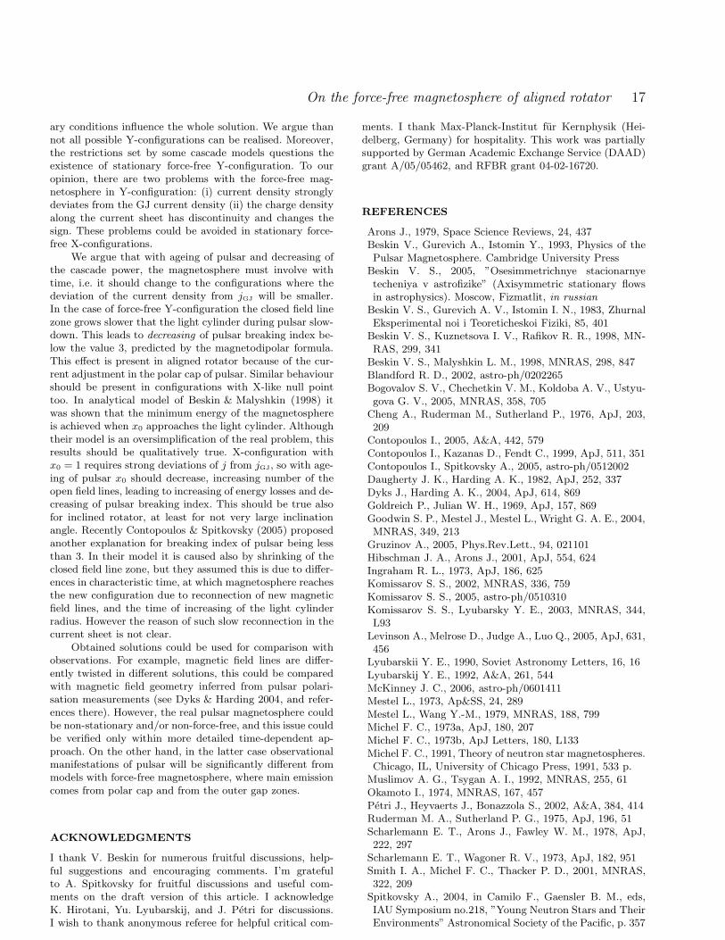
On the force-free magnetosphere of aligned rotator 17
ary conditions influence the whole solution. We argue thannot all possible Y-configurations can be realised. Moreover,the restrictions set by some cascade models questions theexistence of stationary force-free Y-configuration. To ouropinion, there are two problems with the force-free mag-netosphere in Y-configuration: (i) current density stronglydeviates from the GJ current density (ii) the charge densityalong the current sheet has discontinuity and changes thesign. These problems could be avoided in stationary force-free X-configurations.
We argue that with ageing of pulsar and decreasing ofthe cascade power, the magnetosphere must involve withtime, i.e. it should change to the configurations where thedeviation of the current density from jGJ will be smaller.In the case of force-free Y-configuration the closed field linezone grows slower that the light cylinder during pulsar slow-down. This leads to decreasing of pulsar breaking index be-low the value 3, predicted by the magnetodipolar formula.This effect is present in aligned rotator because of the cur-rent adjustment in the polar cap of pulsar. Similar behaviourshould be present in configurations with X-like null pointtoo. In analytical model of Beskin & Malyshkin (1998) itwas shown that the minimum energy of the magnetosphereis achieved when x0 approaches the light cylinder. Althoughtheir model is an oversimplification of the real problem, thisresults should be qualitatively true. X-configuration withx0 = 1 requires strong deviations of j from jGJ, so with age-ing of pulsar x0 should decrease, increasing number of theopen field lines, leading to increasing of energy losses and de-creasing of pulsar breaking index. This should be true alsofor inclined rotator, at least for not very large inclinationangle. Recently Contopoulos & Spitkovsky (2005) proposedanother explanation for breaking index of pulsar being lessthan 3. In their model it is caused also by shrinking of theclosed field line zone, but they assumed this is due to differ-ences in characteristic time, at which magnetosphere reachesthe new configuration due to reconnection of new magneticfield lines, and the time of increasing of the light cylinderradius. However the reason of such slow reconnection in thecurrent sheet is not clear.
Obtained solutions could be used for comparison withobservations. For example, magnetic field lines are differ-ently twisted in different solutions, this could be comparedwith magnetic field geometry inferred from pulsar polari-sation measurements (see Dyks & Harding 2004, and refer-ences there). However, the real pulsar magnetosphere couldbe non-stationary and/or non-force-free, and this issue couldbe verified only within more detailed time-dependent ap-proach. On the other hand, in the latter case observationalmanifestations of pulsar will be significantly different frommodels with force-free magnetosphere, where main emissioncomes from polar cap and from the outer gap zones.
ACKNOWLEDGMENTS
I thank V. Beskin for numerous fruitful discussions, help-ful suggestions and encouraging comments. I’m gratefulto A. Spitkovsky for fruitful discussions and useful com-ments on the draft version of this article. I acknowledgeK. Hirotani, Yu. Lyubarskij, and J. Petri for discussions.I wish to thank anonymous referee for helpful critical com-
ments. I thank Max-Planck-Institut fur Kernphysik (Hei-delberg, Germany) for hospitality. This work was partiallysupported by German Academic Exchange Service (DAAD)grant A/05/05462, and RFBR grant 04-02-16720.
REFERENCES
Arons J., 1979, Space Science Reviews, 24, 437Beskin V., Gurevich A., Istomin Y., 1993, Physics of thePulsar Magnetosphere. Cambridge University Press
Beskin V. S., 2005, ”Osesimmetrichnye stacionarnyetecheniya v astrofizike” (Axisymmetric stationary flowsin astrophysics). Moscow, Fizmatlit, in russian
Beskin V. S., Gurevich A. V., Istomin I. N., 1983, ZhurnalEksperimental noi i Teoreticheskoi Fiziki, 85, 401
Beskin V. S., Kuznetsova I. V., Rafikov R. R., 1998, MN-RAS, 299, 341
Beskin V. S., Malyshkin L. M., 1998, MNRAS, 298, 847Blandford R. D., 2002, astro-ph/0202265Bogovalov S. V., Chechetkin V. M., Koldoba A. V., Ustyu-gova G. V., 2005, MNRAS, 358, 705
Cheng A., Ruderman M., Sutherland P., 1976, ApJ, 203,209
Contopoulos I., 2005, A&A, 442, 579Contopoulos I., Kazanas D., Fendt C., 1999, ApJ, 511, 351Contopoulos I., Spitkovsky A., 2005, astro-ph/0512002Daugherty J. K., Harding A. K., 1982, ApJ, 252, 337Dyks J., Harding A. K., 2004, ApJ, 614, 869Goldreich P., Julian W. H., 1969, ApJ, 157, 869Goodwin S. P., Mestel J., Mestel L., Wright G. A. E., 2004,MNRAS, 349, 213
Gruzinov A., 2005, Phys.Rev.Lett., 94, 021101Hibschman J. A., Arons J., 2001, ApJ, 554, 624Ingraham R. L., 1973, ApJ, 186, 625Komissarov S. S., 2002, MNRAS, 336, 759Komissarov S. S., 2005, astro-ph/0510310Komissarov S. S., Lyubarsky Y. E., 2003, MNRAS, 344,L93
Levinson A., Melrose D., Judge A., Luo Q., 2005, ApJ, 631,456
Lyubarskii Y. E., 1990, Soviet Astronomy Letters, 16, 16Lyubarskij Y. E., 1992, A&A, 261, 544McKinney J. C., 2006, astro-ph/0601411Mestel L., 1973, Ap&SS, 24, 289Mestel L., Wang Y.-M., 1979, MNRAS, 188, 799Michel F. C., 1973a, ApJ, 180, 207Michel F. C., 1973b, ApJ Letters, 180, L133Michel F. C., 1991, Theory of neutron star magnetospheres.Chicago, IL, University of Chicago Press, 1991, 533 p.
Muslimov A. G., Tsygan A. I., 1992, MNRAS, 255, 61Okamoto I., 1974, MNRAS, 167, 457Petri J., Heyvaerts J., Bonazzola S., 2002, A&A, 384, 414Ruderman M. A., Sutherland P. G., 1975, ApJ, 196, 51Scharlemann E. T., Arons J., Fawley W. M., 1978, ApJ,222, 297
Scharlemann E. T., Wagoner R. V., 1973, ApJ, 182, 951Smith I. A., Michel F. C., Thacker P. D., 2001, MNRAS,322, 209
Spitkovsky A., 2004, in Camilo F., Gaensler B. M., eds,IAU Symposium no.218, ”Young Neutron Stars and TheirEnvironments” Astronomical Society of the Pacific, p. 357
c© RAS, MNRAS 000, 1–19

18 A. N. Timokhin
Spitkovsky A., 2005, in T. Bulik B. Rudak G. M., ed., ”AS-TROPHYSICAL SOURCES OF HIGH ENERGY PAR-TICLES AND RADIATION” Vol. 801 of AIP ConferenceProceedings. p. 253
Spitkovsky A., Arons J., 2002 Vol. 271 of ASP ConferenceSeries. p. 81
Spitkovsky A., Arons J., 2004, ApJ, 603, 669Sturrock P. A., 1971, ApJ, 164, 529Sulkanen M. E., Lovelace R. V. E., 1990, ApJ, 350, 732Takata J., Shibata S., Hirotani K., 2004, MNRAS, 354,1120
Timokhin A. N., 2005, astro-ph/0507054Trottenberg U., Oosterlee C. W., Schuller A., Brandt A.,Oswald P., Stuben K., 2001, Multigrid. Academic Press
Uzdensky D. A., 2003, ApJ, 598, 446
APPENDIX A: CURRENT DENSITY IN THE
POLAR CAP
The poloidal current density is given by (see Beskin 2005)
jpol =∆I × eφ
=
dI
dΨBpol , (A1)
the latter expression was obtained by taking into accountrelation (10). Substituting for Bpol the expression for thedipole magnetic field at the NS surface Bpol = B0(er cos θ+(1/2)eθ sin θ) and expressing I and Ψ through normalisedquantities we get for the poloidal current density in the polarcap of pulsar
jpc = |jGJ| 12S′(ψ)
√
1− 3
4sin2 θ , (A2)
where |jGJ| is the absolute value of the Goldreich-Julian cur-rent density in the polar cap
|jGJ| =B0Ω
2πcc . (A3)
For dipole magnetic field in the polar cap (see eq. (44))
ψ =RLC
RNS
sin2 θ ≈ RLC
RNS
θ2 . (A4)
The colatitude of the polar cap boundary is θpc = 1.45 ×10⁻²P−1/2√ψlast, P is period of pulsar in seconds. So,θ2 < θ2pc ≪ 1 and the term with sin2 θ in eq.(A2) can beneglected. From equation (A4) we have relation between thecolatitude θ in the polar cap and the corresponding magneticflux function ψ
ψ = ψlast
(
θ
θpc
)2
. (A5)
Substituting this relation into equation (A2) we get
jpc = |jGJ| 12S′(
(
θ
θpc
)2
ψlast) . (A6)
APPENDIX B: ENERGY LOSSES
The poloidal component of Poynting flux in the magneto-sphere of aligned rotator is
P pol =c
4π[E×B]pol = −ΩF
cIBpol , (B1)
the latter expression was obtained with help of eqs. (8),(14).Expressing Bpol through Ψ, eq. (9), we have for the radialcomponent of the Poynting flux
Pr = − IΩF
c
1
r(Z ∂Ψ−∂ZΨ) , (B2)
where r =√2 + Z2. Energy losses trough a soling angle
dω are dW = −r2Pr dω. The angular distribution of energylosses are given by
dW
dω=IΩF
c
r
(Z ∂Ψ−∂ZΨ) . (B3)
Using normalised quantities we rewrite this equation as
dW
dω=
|Wmd|4π
S
√x2 + z2
x(z ∂xψ − x ∂zψ) , (B4)
where |Wmd| is absolute value of magnetodipolar energylosses, here defined as
|Wmd| ≡µ2
R4LC
c =B2
0R6NSΩ
4
4c3. (B5)
Energy losses of aligned rotator can be obtained by in-tegration of equation (B3):
W =
∫
4π
dW
dωdω = 2
∫ Ψlast
0
2π
cIΩF dΨ , (B6)
factor 2 appears because energy is carried away by thePoynting flux from both hemispheres. Using normalisedquantities introduced at the end of the section 2.1 this for-mula can be rewritten as
W =µ2
R4LC
c
∫ ψlast
0
S dψ = |Wmd|∫ ψlast
0
S dψ . (B7)
Analytical formula for estimation of aligned rotator en-ergy losses could be obtained on the following way. Poloidalcurrent S for each of obtained solutions does not deviatesmuch from the Michel’s current function, eq.(50). Substitut-ing this function into equation (B7) we get
W ≈ −2
3ψ2
last |Wmd| . (B8)
Dependence of ψlast on x0 we could estimate using mag-netic flux function of the dipolar field, eq.(19). Substitutingψdip(x0) = x−1
0 into equation (B8) we get
W ≈ −2
3x−20 |Wmd| . (B9)
APPENDIX C: THE SIZE OF THE REGION
WHERE PARTICLE INFLOW IS POSSIBLE
Charged particles in crossed electric and magnetic fields driftwith the velocity UD given by eq. (16), which can be rewrit-ten as
UD =ΩF
B2(B2
poleφ −BφBpol) . (C1)
In general, charged particle in the magnetosphere could havetwo velocity components: one perpendicular to the magneticfield line (the drift velocity) and an additional componentalong magnetic field line U||, see Fig. C1. With increasingof the distance from the NS UD increases, see Fig. 3. Thevelocity of the particle U can not exceed the speed of light,
c© RAS, MNRAS 000, 1–19

On the force-free magnetosphere of aligned rotator 19
PSfrag replacements
~U
Ur
~UD
UD r
U||
U|| rα
Br
~B
r
Figure C1. Particle velocity decomposition in U|| and UD. Mag-netic field line is shown by the thick curved line.
hence, the parallel component of particle velocity far fromNS must be also smaller. Magnetic field lines far from NSare strongly twisted and at some distance the particle radialvelocity component will be positive, i.e. directed from theNS, for any direction of the parallel component. At thesedistances particles can flow only from the NS. Let us showthat the size of the domain, where particles could flow tothe NS, corresponds to the size of the light cylinder.
From Fig. C1 it is evident that the radial component ofthe total particle velocity is
Ur = UD r + U|| r . (C2)
The maximal value of the velocity component parallel to themagnetic field is
Umax|| ≃
√
c2 −U 2D . (C3)
If the radial component of the magnetic field Br > 0 thenfor the azimuthal component of magnetic field Bφ = −|Bφ|.For radial components of particle velocities we have
Umax|| r = −Br
BUmax
|| ≃ −BrBc
√
1−(
ΩF
c
)2 B2pol
B2(C4)
UD r =ΩF
B2|Bφ|Br (C5)
From this the maximal possible velocity component in radialdirection is
Umaxr ≃ −Br
Bc
(√
1−(
ΩF
c
)2 B2pol
B2− ΩF
c
|Bφ|B
)
(C6)
Particles could flow to the NS only if Umaxr < 0, and this is
possible if√
1−(
ΩF
c
) B2pol
B2>
ΩF
c
|Bφ|B
(C7)
or
<c
ΩF
, (C8)
i.e. only inside the light cylinder. For Br < 0 we get the sameresult. The same restriction, namely that particles could
cross the alfvenic surface (light cylinder in our case) onlyin one direction, is proved to be valid in full MHD case too(see e.g. Beskin 2005).
c© RAS, MNRAS 000, 1–19


