On-the-fly Modelling and Prediction of Epidemic … College London Department of Computing...
76
Imperial College London Department of Computing On-the-fly Modelling and Prediction of Epidemic Phenomena Author: Ionela Roxana D˘ anil˘ a Supervisor: Dr. William Knottenbelt Co-supervisor: PhD student Marily Nika Second marker: Dr. Jeremy BRADLEY A thesis submitted in fulfilment of the requirements for the degree of Master of Engineering in Computing June 2014
Transcript of On-the-fly Modelling and Prediction of Epidemic … College London Department of Computing...
Imperial College LondonDepartment of Computing
On-the-fly Modelling and Prediction ofEpidemic Phenomena
Author:Ionela Roxana Danila
Supervisor:Dr. William Knottenbelt
Co-supervisor:PhD student Marily Nika
Second marker:Dr. Jeremy BRADLEY
A thesis submitted in fulfilment of the requirements for the degree ofMaster of Engineering in Computing
June 2014

“I simply wish that, in a matter which so closely con-cerns the wellbeing of the human race, no decision shall bemade without all the knowledge which a little analysis andcalculation can provide.”
Daniel Bernoulli, 1760
Abstract
The modern world features a plethora of social, technological and biological epidemicphenomena. These epidemics now spread at unprecedented rates thanks to advances inindustrialisation, transport and telecommunications. Effective real-time decision makingand management of modern epidemic outbreaks based on model analysis depends on twofactors: the ability to estimate epidemic parameters as the epidemic unfolds, and theability to characterise rigorously the uncertainties surrounding these parameters. In thiscontext, uncertainty should be understood as a statement about how well something isknown, rather than being regarded as the act of not knowing.
The main contribution of this project is a generic Maximum Likelihood based approachtowards on-the-fly epidemic fitting of SIR models from a single trace, which yields con-fidence intervals on parameter values. In contrast to traditional biological modellingtechniques, our approach is fully automated and the parameters to be estimated includethe initial number of susceptible and infected individuals in the population. Visualisingthe fitted parameters gives rise to an isosurface plot of the feasible parameter rangescorresponding to each confidence level.
We validated our methodology on both synthetic datasets generated using stochasticsimulation, and real Influenza data. Fitting parameters to those trajectories revealedremarkable results. The model proved highly accurate in predicting from partial infor-mation on a single trace not only the time of the peak, but also its magnitude, and thetail of the infection. However, the “true” parameters were contained in the correspond-ing confidence bounds only for a relatively low proportion of the time, emphasising (a)the difficulty of obtaining accurate parameter estimations from a single epidemic traceand (b) the large potential impact of small random variations, especially those occurringearly on in a trace.

Acknowledgements
First and foremost, I would like to thank to Dr. William Knottenbelt, his PhD studentMarily Nika, and Dr. Jeremy Bradley for the input and guidance they have given methrough the course of the project. Their dedication and passion for the subject weretruly inspiring and contagious.
Secondly, I would also like to thank to my personal tutor, Prof. John Darlington, and toMrs. Margaret Cunningham for their pastoral care and encouragement provided duringmy studies.
Last but not least, I would like to thank my parents for their continuous care and supportthroughout the years. Without them I would have not been able to pursue my dreamsand to become the person I am today.

Contents
Abstract i
Acknowledgements ii
Contents ii
1 Introduction 11.1 Motivation . . . . . . . . . . . . . . . . . . . . . . . . . . . . . . . . . . . 21.2 Objectives . . . . . . . . . . . . . . . . . . . . . . . . . . . . . . . . . . . . 41.3 Contributions . . . . . . . . . . . . . . . . . . . . . . . . . . . . . . . . . . 41.4 Report outline . . . . . . . . . . . . . . . . . . . . . . . . . . . . . . . . . 5
2 Background 62.1 Control of Epidemics . . . . . . . . . . . . . . . . . . . . . . . . . . . . . . 6
2.1.1 Traditional Methods . . . . . . . . . . . . . . . . . . . . . . . . . . 72.1.2 Mathematical Modelling . . . . . . . . . . . . . . . . . . . . . . . . 8
2.2 Deterministic Compartmental Models . . . . . . . . . . . . . . . . . . . . 112.2.1 SIR model . . . . . . . . . . . . . . . . . . . . . . . . . . . . . . . . 112.2.2 Other Models . . . . . . . . . . . . . . . . . . . . . . . . . . . . . . 142.2.3 Basic Reproductive Ratio . . . . . . . . . . . . . . . . . . . . . . . 162.2.4 Epidemic Burnout . . . . . . . . . . . . . . . . . . . . . . . . . . . 18
2.3 Uncertainty Sources . . . . . . . . . . . . . . . . . . . . . . . . . . . . . . 192.3.1 Stochastic Uncertainty . . . . . . . . . . . . . . . . . . . . . . . . . 192.3.2 Parameter Uncertainty . . . . . . . . . . . . . . . . . . . . . . . . . 20
2.4 Other Applications of Epidemiological Models . . . . . . . . . . . . . . . . 202.4.1 Social Network Analysis . . . . . . . . . . . . . . . . . . . . . . . . 202.4.2 Economic cycles . . . . . . . . . . . . . . . . . . . . . . . . . . . . 202.4.3 Retail Sales . . . . . . . . . . . . . . . . . . . . . . . . . . . . . . . 222.4.4 Computer Viruses . . . . . . . . . . . . . . . . . . . . . . . . . . . 22
2.5 Development Environment . . . . . . . . . . . . . . . . . . . . . . . . . . . 242.5.1 Programming Language . . . . . . . . . . . . . . . . . . . . . . . . 242.5.2 Additional Libraries and Tools . . . . . . . . . . . . . . . . . . . . 25
3 Fitting Procedure using Least Squares 263.1 Model . . . . . . . . . . . . . . . . . . . . . . . . . . . . . . . . . . . . . . 263.2 Objective Function . . . . . . . . . . . . . . . . . . . . . . . . . . . . . . . 293.3 Optimisation Technique . . . . . . . . . . . . . . . . . . . . . . . . . . . . 303.4 Goodness of Fit . . . . . . . . . . . . . . . . . . . . . . . . . . . . . . . . . 31
iii

Contents iv
4 Uncertainty Characterisation using Maximum Likelihood 324.1 Objective Function . . . . . . . . . . . . . . . . . . . . . . . . . . . . . . . 334.2 Optimisation Technique . . . . . . . . . . . . . . . . . . . . . . . . . . . . 344.3 Confidence Intervals . . . . . . . . . . . . . . . . . . . . . . . . . . . . . . 354.4 New Approach for Uncertainty Characterisation . . . . . . . . . . . . . . . 39
4.4.1 Data Transformation . . . . . . . . . . . . . . . . . . . . . . . . . . 394.4.2 Parameter Space Searching . . . . . . . . . . . . . . . . . . . . . . 404.4.3 Visualisation . . . . . . . . . . . . . . . . . . . . . . . . . . . . . . 41
5 Evaluation 435.1 Synthetic Data . . . . . . . . . . . . . . . . . . . . . . . . . . . . . . . . . 43
5.1.1 Fitting Using Least Squares . . . . . . . . . . . . . . . . . . . . . . 445.1.2 Fitting Using Maximum Likelihood . . . . . . . . . . . . . . . . . . 47
5.2 CDC Influenza Data . . . . . . . . . . . . . . . . . . . . . . . . . . . . . . 565.2.1 Fitting Using Least Squares . . . . . . . . . . . . . . . . . . . . . . 565.2.2 Fitting Using Maximum Likelihood . . . . . . . . . . . . . . . . . . 59
6 Conclusion 646.1 Contributions . . . . . . . . . . . . . . . . . . . . . . . . . . . . . . . . . . 646.2 Future Work . . . . . . . . . . . . . . . . . . . . . . . . . . . . . . . . . . 65
Bibliography 66

Chapter 1
Introduction
As far as the laws of mathematics refer to reality, they are not certain; andas far as they are certain, they do not refer to reality.
Albert Einstein
This project investigates uncertainty in epidemic modelling and presents a generic, fullyautomated method for on-the-fly epidemic fitting of SIR models from a single trace.It yields confidence intervals on parameter values that rigorously characterise the un-certainty inherent in their estimates. The modern era features a plethora of social,technological and biological epidemic phenomena. They spread at unprecedented ratesdue to advances in technology, transport and telecommunications. Mathematical mod-elling plays a key role in effective real-time decision making and management of modernepidemic outbreaks.
The ability to characterise uncertainty is absolutely critical in the context of policy anddecision making. There is a popular misconception around the meaning of the term.Uncertainty is often regarded as not knowing. However, when it comes to decision mak-ing, it should be understood as a statement about how well something is known. As ageneral rule, uncertainty is inherent in science. Thus, to ignore or to minimise acknowl-edging its existence practically means to ignore science. Usually, there is a temptationto either focus only on the best estimates and ignore the less likely results, or to onlyconsider the highly unlikely results based on extremely cautious assumptions. Both ofthese two approaches may lead to poor decision making. Instead, we should attempt todescribe how far from the truth any given estimate is likely to be. Moreover, interpretingand framing of uncertainty may be subject to people’s biases. It is therefore extremelyimportant to develop a rigorous, scientific method that characterises uncertainty.
1
Chapter 1. Introduction 2
1.1 Motivation
Movement of disease constituted a major force in shaping the human history, with warsand migrations carrying infections to susceptible populations. Before World War II, morevictims died due to microbes introduced by the enemy, than of battle wounds [1]. Thiswas still a period of relative isolation across different communities. More recent timeshave allowed extensive contact between people around the world. Modern transportnetworks continuously expand in reach, speed of travel and volume of passengers carried,causing epidemics to spread further and faster than ever before. In the 14th century, theBlack Death travelled between 1 and 5 miles a day on average [2]. On the other hand,the severe acute respiratory syndrome outbreak of 2003 transmitted from Hong Kong toHanoi, Singapore and Toronto within just a few days after the first infected case [3].
Gladwell [4] states that ideas, products, messages and behaviours spread in a similarmanner to viruses, leading to social and technological epidemics. These phenomena areeven more invasive due to the extensive coverage of internet and social media. Even so,they are based on the same three principles that explain how measles spread or why fluoutbreaks occur every winter. Firstly, they have a contagious nature. Secondly, theymay be triggered by seemingly inconsequential causes. Lastly and most important, thereis one dramatic moment, the tipping point, when they begin to spread.
Our understanding of infectious disease dynamics has greatly improved in recent yearsthanks to mathematical modelling. Insights from this increasingly-important field en-able policy-makers at the highest levels to interpret and evaluate data, in order tocomprehend and predict transmission patterns. Compartmental models are widely usedin epidemiology, allowing us to target control measures and use limited resources moreefficiently. They reduce the population diversity to a few key characteristics, relevantto the phenomenon studied. For example, one of the most widely-known such modelsis SIR, which divides the population in susceptible, infected and recovered individuals.Parameters such as the rate of infection and the rate of recovery determine the behaviourof the model, but cannot be measured directly, hence they must be estimated in someway. Ultimately, the quality of a model is highly dependent on both the data used forparameterisation and the uncertainty present in the model outcomes.
One source of unreliability may arise when the data sets used for analysis are not entirelyrelevant to the hypothesis to test. A recent study published by two PhD studentsat Princeton University [5] states that Facebook will lose 80% of its users by 2017.One of the critical errors made in this non-peer-reviewed paper comes from applying a“correlation equals causation” principle. They deduced that a decline in the volume ofGoogle searches for “Facebook” causes an ongoing decline in Facebook usage. However,

Chapter 1. Introduction 3
this decline does not prove anything considering that over half of Facebook’s traffic comesfrom their mobile application at present. Indeed, since 2012, the number of active userskept growing, reaching today almost 1.2 billions [6]. Another source of error in theirresults is considering the Facebook phenomenon as a single outbreak, that starts byexponentially “infecting” people who then ultimately recover, causing the extinction ofthe epidemic. The user engagement strategy may be seen as a virus, but its mutationsmust not be omitted. In order to keep the engagement rates high, the company willcontinuously find new ways of attracting more users, generating each time new socialand technological outbreaks.
Additionally, models are often developed and presented with insufficient attention tothe uncertainties that underlie them. The authors of a recent study [7] analysed sci-entific papers, interviews, policies, reports and outcomes of previous infectious diseaseoutbreaks in the United Kingdom. An extract from one of the scientific papers relatedto the dynamics of the 2001 UK foot and mouth epidemic is reproduced below:
“Relative infectivity and susceptibility of sheep and cattle. Experimental results agreewith the pattern of species differences used within the model. Quantitative changes tothe species parameters will modify the predicted spatio-temporal distribution of outbreaks;our parameters have been chosen to give the best match to the location of high risk areas.However this choice of parameters is contingent on the accuracy of the census distributionof animals on farms.”
The purpose of their research was to ascertain the role uncertainties played in previ-ous models, and how these were understood by both the designers and the users of themodel. They found that many models provided only cursory reference to the uncertain-ties inherent in the parameters used. The study concludes that greater considerationof the limitations and uncertainties in infectious disease modelling would improve itsusefulness and value.
Models provide epidemiologists with an environment able to record every detail of thedisease spread, such that each individual component can be analysed in isolation tothe whole system. However, every model has its limitations. There will always bean unknown or unknowable element in the system. For example, if we try to modelInfluenza, we need to account for factors such as movement and interaction of individuals,variability in susceptibility due to past infections, variations in transmission patternscaused by temperature and many more. We cannot capture all the different scenariosin order to predict the precise evolution of the epidemic. Instead, we should aim forproviding confidence intervals on the parameters that determine the behaviour of theepidemic.
Chapter 1. Introduction 4
1.2 Objectives
The project aims to undertake on-the-fly parameter fitting as an epidemic unfolds, givenregular observations in time of the number of infected individuals, and characterise theuncertainty inherent in the parameter estimates.
We will first consider least-squares-based techniques for parameter fitting to predict thefuture evolution of the epidemic, and answer questions such as “when will it peak?”,“when will it have died out?”, “how many people will be infected at a particular pointin time”, or “how many people need to be vaccinated to prevent an epidemic?”
Further, we aim to develop a rigorous maximum-likelihood-based methodology of charac-terising uncertainty. We consider uncertainty that comes from two sources: the stochas-tic evolution of the epidemic, and the parameters values, which are often unknown orimprecise. Traditional approaches used in biological epidemics require laborious manualwork for index case identification, laboratory testing, contact tracing and report aggre-gation. The project will investigate to what extent a fully automated method could bedeployed and, if possible, implement it.
We consider the challenges of estimating the initial number of susceptible and infectedindividuals in the target population, when these values are unknown. Currently, there isno principled way of doing this, as traditionally they are either supposed to be known,or can be estimated from the context [8]. However, in an era of social and technologicalepidemics, we argue that time and speed of movement make it infeasible to provideaccurate estimates.
1.3 Contributions
This project made the following contributions:
• Investigation of on-the-fly parameters fitting as an epidemic unfolds, from a singletrace using compartmental models.
• Implementation of a least-squares-based methodology for data fitting on SIR model,as en epidemic unfolds over time, tackling the challenge of unknown initial numberof susceptibles.
• Implementation of a novel, fully automated maximum-likelihood-based methodol-ogy for data fitting on SIR model, as en epidemic unfolds over time, that provides
Chapter 1. Introduction 5
rigorous characterisation of uncertainty inherent in parameter estimates. We con-sider the challenges of applying this procedure when the initial number of suscep-tibles and infected individuals is unknown.
• A three-dimensional visualisation of the confidence intervals characterising param-eters uncertainty in the SIR model when the number of susceptibles is unknown.
• Validation of the methodologies on both synthetic and real data.
• A paper co-authored with Thomas Wilding, Marily Nika and Dr. William Knotten-belt, and submitted to EPEW 2014, the 11th European Workshop on PerformanceEngineering, taking place in Florence, Italy, between 11-12 September 2014.
1.4 Report outline
Chapter 2 presents background information regarding infectious disease modelling. First,it introduces the laborious manual techniques traditionally used in developing diseasecontrol strategies. Subsequently, it highlights the role of mathematical modelling inepidemiology and describes in detail the main compartmental models widely used in thisfield. Further, it presents the main sources of uncertainty these models must accountfor. Next, an overview of other areas where compartmental models can be applied isgiven. Finally, we outline the main design decisions made regarding the programminglanguage and additional libraries used to run the experiments.
Chapter 3 describes a least-squares based methodology for on-the-fly epidemic fittingon the SIR model, from a single trace. It provides mathematical details concerning theobjective function, the optimisation technique, and the assessment of goodness of fit.
Chapter 4 introduces a novel, generic, and fully automated maximum-likelihood-basedmethodology for on-the-fly epidemic fitting on SIR models, from a single trace, thatyields confidence intervals on parameter values. It represents a rigorous characterisa-tion of the uncertainty inherent in parameter estimates. We first give mathematicaldetails of the objective function, the optimisation technique, and the computation ofconfidence intervals. Then, we describe how we applied the methodology step-by-stepfor various vectors of unknown parameters. Finally, a three-dimensional visualisation ofthe confidence intervals is given, when dealing with three unknown parameters.
Chapter 5 presents the results of validating our methodologies on both synthetic andreal data and a detailed discussion of their interpretation.
Chapter 6 concludes with a summary of the achievements and a discussion on futurework.
Chapter 2
Background
2.1 Control of Epidemics
Improving control strategies and eradicating the disease from a population are the pri-mary reasons behind studying infectious diseases. The Oxford English Dictionary definesan epidemic as “a widespread occurrence of an infectious disease in a community at aparticular time.” It can be described as a sudden outbreak of a disease, infecting asignificant percentage of a population, that eventually disappears, usually leaving someof the individuals untouched. Management of epidemics involves a series of activities,from forecasting to investigation, control and prevention of future occurrences.
Traditional methods for disease control are applied after the extinction of an epidemic inorder to better understand its dynamics from empirical data. These techniques have thepotential of being highly efficient when dealing with a small number of cases. However,they become very tedious at a higher scale due to the laborious manual work usuallyinvolved, as discussed in Section 2.1.1.
During the course of an epidemic, it is extremely important to be able to predict thefuture course of the outbreak in real-time. In this context, prediction should be under-stood as both a quantitative approach, and an attempt of inferring what would happenunder certain assumptions. Forecasting may not lead to a complete prevention of theepidemic, but it can control its severity and spread. Mathematical modelling plays amajor role in accomplishing this, as discussed in section 2.1.2.
6
Chapter 2. Background 7
2.1.1 Traditional Methods
Traditionally, disease control strategies are developed after a series of laborious manualefforts. Epidemiologists collect data on symptoms, past medical history, laboratorytesting, exam findings, and recent treatments that an infected individual have received,and also trace contacts between individuals. The aim is to identify the index case andthe transmission network of the infection in order to understand its dynamics and makeinformed decisions for future prevention.
In epidemiology, an index case, also referred as patient zero, is considered to be the firstdocumented case of a disease. Identifying these cases as soon as possible can providesignificant information about the origin of the outbreak. It is also important to trace thepathways of the disease and construct its transmission network, which highlights detailson how the disease spread. Infection tracing is an integral component of post-epidemicdisease control policies. It aims to determine the source of infection for each case. Thebasic idea is to link each infected individual to both the one whom it caught the diseasefrom, and the ones to whom they transmitted it to. In this way, the transmission networkcan be built. We discuss below the main traditional methods used to collect the requiredinformation.
Contact Tracing
Contact tracing is the process of identifying individuals who came in contact with aninfected person. It aims to determine all potential transmission contacts from the indexcase. This methodology has many limitation. Firstly, it is highly laborious intensiveand time consuming. Additionally, it fully relies on individuals being able to recall andprovide complete, accurate information regarding their personal relationships.
Diary-based Studies
In contrast to contact tracing, diary-based studies attempt to record individual contactsas they occur. The advantage of this strategy is that the workload is shifted fromresearchers to the subjects, allowing a larger number of individuals to be tracked [9].However, it also has a series of disadvantages. Firstly, the data collected is still at thediscretion of individuals, hence its accuracy and consistency may vary. Secondly, itcan be difficult for the coordinating researcher to organise all the information, as theidentifiers of the contacts recorded may not be consistent.
Chapter 2. Background 8
2.1.2 Mathematical Modelling
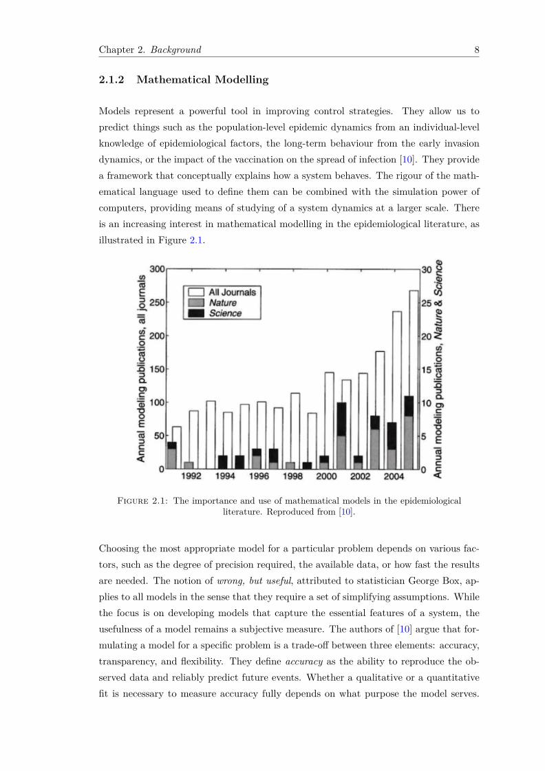
Models represent a powerful tool in improving control strategies. They allow us topredict things such as the population-level epidemic dynamics from an individual-levelknowledge of epidemiological factors, the long-term behaviour from the early invasiondynamics, or the impact of the vaccination on the spread of infection [10]. They providea framework that conceptually explains how a system behaves. The rigour of the math-ematical language used to define them can be combined with the simulation power ofcomputers, providing means of studying of a system dynamics at a larger scale. Thereis an increasing interest in mathematical modelling in the epidemiological literature, asillustrated in Figure 2.1.
Figure 2.1: The importance and use of mathematical models in the epidemiologicalliterature. Reproduced from [10].
Choosing the most appropriate model for a particular problem depends on various fac-tors, such as the degree of precision required, the available data, or how fast the resultsare needed. The notion of wrong, but useful, attributed to statistician George Box, ap-plies to all models in the sense that they require a set of simplifying assumptions. Whilethe focus is on developing models that capture the essential features of a system, theusefulness of a model remains a subjective measure. The authors of [10] argue that for-mulating a model for a specific problem is a trade-off between three elements: accuracy,transparency, and flexibility. They define accuracy as the ability to reproduce the ob-served data and reliably predict future events. Whether a qualitative or a quantitativefit is necessary to measure accuracy fully depends on what purpose the model serves.
Chapter 2. Background 9
Gaining insight into the dynamics of the disease would require a qualitative fit, whileestablishing control policies would rather use a quantitative approach. The accuracy of amodel is limited by computational feasibility, the modeller’s understanding of the systemin question, and the knowledge of the necessary parameters. Transparency is regardedas the ability to understand how the individual components of the system interact andinfluence the dynamics of the whole. The level of transparency usually decreases withthe number of model components, as it becomes increasingly difficult to account for therole of each individual component. Finally, they define flexibility as a measure of howeasily the model can be adapted to new situations. This proves to be essential whenmodelling diseases in an ever-changing environment.
According to [11], models can play three major roles in informing policy: prediction,extrapolation, and experimentation. Predictive models take a set of initial conditionsand attempt to determine the future evolution of the epidemic, such as its size andlocation, in order to enforce appropriate control strategies. Models can also be used toconstruct the probable dynamics of a disease for a set of parameters by extrapolatingfrom the known dynamics for another set of parameters. This can be useful when weare interested in studying the effects of relaxing or enhancing the control measures.Finally, models can be used to test various control strategies in a short period of time,by avoiding all the risks associated with testing during a real epidemic. One of the firsttimes that models were used to support decision making during an epidemic was the2001 foot-and-mouth disease outbreak in the UK. Three different models were used toinvestigate whether the epidemic was under control and assess to what extent targetedculling would be effective in reducing the spread of infection, in order to inform controlmeasures.
No model is perfect and able to precisely predict the exact evolution of an epidemic.However, a good model is defined by two principles [10]. Firstly, it should be suited toits purpose. This means it should have a good balance of accuracy, transparency andflexibility. In other words, it must be as simple as possible, but no simpler, as it is oftenquoted in literature. Secondly, it should be parametrizable from available data for eachof the features included. Hence, the definition of a good model is highly dependent onthe context.
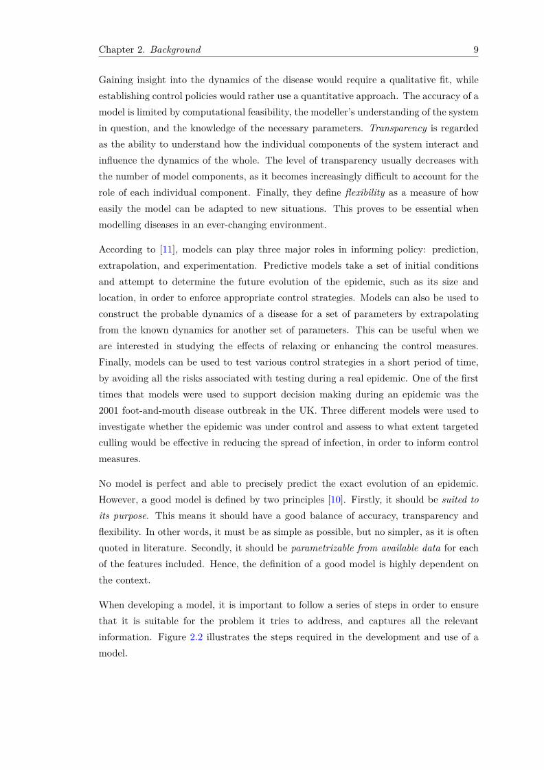
When developing a model, it is important to follow a series of steps in order to ensurethat it is suitable for the problem it tries to address, and captures all the relevantinformation. Figure 2.2 illustrates the steps required in the development and use of amodel.
Chapter 2. Background 10
Identify the question
Identify relevant facts about the infecton in question
Choose type of modelling method
Specify model input parameters
Set up model
Model validation
Prediction and optimisation
Figure 2.2: Steps in the development and use of a model. Adapted from [12].
Mathematical modelling has a long history in epidemiology. The first known result datesback from 1760 and is attributed to Daniel Bernoulli. It was an early attempt to statis-tically analyse the mortality caused by smallpox and defend the benefits of vaccinationagainst it, a matter heavily debated at the time. In terms of modern mathematicalepidemiology, the first contributions were made in the late 1880s, by Piotr DimitrievichEn’ko, a Russian physician whose probabilistic modelling and data analysis of measlesepidemics anticipated the work of Reed and Frost in the 1920s.
One of the early triumphs in epidemiology is the approach based on simple compartmen-tal models, developed between 1900 and 1935, having as contributors R.A. Ross, W.H.Hamer, A.G. McKendrick, W.O. Kermack and J. Brownlee. Compartmental modelsrely on two main assumptions. Firstly, it is assumed that the population under analysiscan be divided into a set of compartments, depending on the stage of the disease de-velopment. Secondly, individuals are asserted to have equal probability to transit fromone compartment to another. There are various questions that these models help usanswer, including “how many individuals will be affected altogether and thus requiretreatment?”, “what is the maximum number of people needing care at any particulartime?” or “how long will the epidemic last?” [12].
Chapter 2. Background 11
2.2 Deterministic Compartmental Models
In a deterministic model, each state is uniquely determined by the parameters of themodel, together with the previous state. Hence, for the same initial conditions, themodel will behave exactly the same, such that each time we would observe an identicaltrajectory corresponding to the evolution of the epidemic.
2.2.1 SIR model
SIR is a compartmental model initially studied in depth by Kermack and McKendrick in1927 [13]. It consists of dividing the population into three subpopulations: Susceptible,Infected and Recovered individuals, and uses Ordinary Differential Equations (ODEs)as a modelling formalism. It defines:
• S(t) the number of individuals who are not yet infected at time t, but susceptibleto become infected
• I(t) the number of individuals who are infected at time t by contact with suscep-tibles at a rate β
• R(t) the number of individuals who have recovered from the disease at time t at aconstant rate γ
The model assumes that the size of each compartment is a differentiable function oftime. It also considers a closed population, ignoring demographic processes such asbirths, deaths and migrations. There are two possible transitions taking place: S →I and I → R. The progression from S to I involves disease transmission at a rate βI,also known as the force of infection, where β is the probability of a contact between asusceptible and an infected individual resulting in infection. It ignores the intricaciesrelated to the pattern of contact between individuals. The transition from I to R occursat a recovery rate γ, assumed to be constant and equal to the inverse of the averageinfectious period.
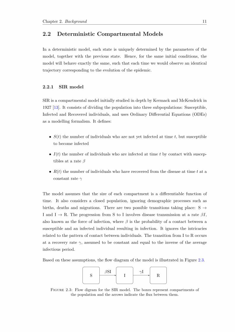
Based on these assumptions, the flow diagram of the model is illustrated in Figure 2.3.
S I RβSI γI
Figure 2.3: Flow digram for the SIR model. The boxes represent compartments ofthe population and the arrows indicate the flux between them.
Chapter 2. Background 12
The assumptions made above can be translated into an initial value problem, definedby the following set of differential equations:
dS
dt= −βSI (2.1)
dI
dt= βSI − γI (2.2)
dR
dt= γI (2.3)
Differential equations used to model the transmission dynamics of a disease describethe events occurring continuously, opposite to difference equations that depict eventstaking place at discrete time intervals. Table 2.1 presents a comparison between differ-ence equations, describing the number of susceptible, infected and recovered individualsat time t, and differential equations, illustrating the rate of change in the number ofindividuals in each compartment at time t.
Difference equations (number) Differential equations (rate)St+1 = St − βtStIt dS
dt = −β(t)S(t)I(t)It+1 = It + βtStIt − γtIt dI
dt = β(t)S(t)I(t)− γ(t)I(t)Rt+1 = Rt + γtIt
dRdt = γ(t)I(t)
Table 2.1: Comparison between difference and differential equations for the SIRmodel.
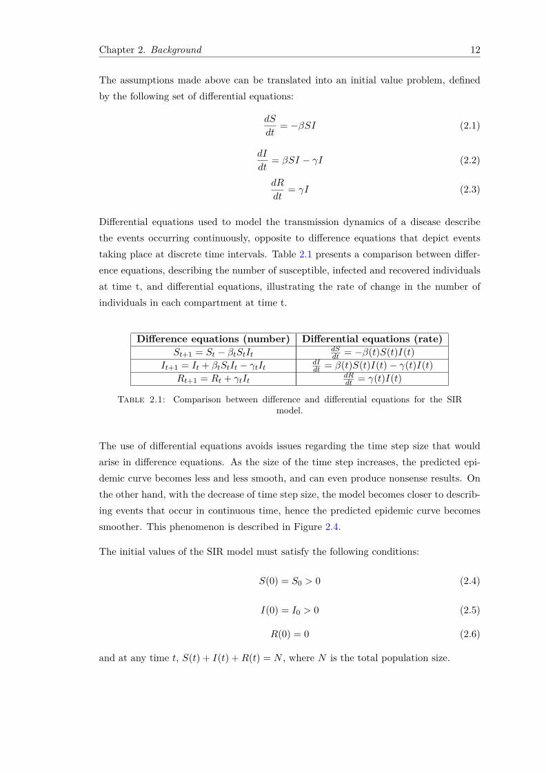
The use of differential equations avoids issues regarding the time step size that wouldarise in difference equations. As the size of the time step increases, the predicted epi-demic curve becomes less and less smooth, and can even produce nonsense results. Onthe other hand, with the decrease of time step size, the model becomes closer to describ-ing events that occur in continuous time, hence the predicted epidemic curve becomessmoother. This phenomenon is described in Figure 2.4.
The initial values of the SIR model must satisfy the following conditions:
S(0) = S0 > 0 (2.4)
I(0) = I0 > 0 (2.5)
R(0) = 0 (2.6)
and at any time t, S(t) + I(t) +R(t) = N , where N is the total population size.
Chapter 2. Background 13
Figure 2.4: Comparison between predictions of the number of infectious individualsfor measles and influenza, using time steps ranging between 0.05 and 5 days. Repro-
duced from [12].
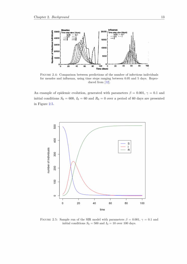
An example of epidemic evolution, generated with parameters β = 0.001, γ = 0.1 andinitial conditions S0 = 600, I0 = 60 and R0 = 0 over a period of 60 days are presentedin Figure 2.5.
Figure 2.5: Sample run of the SIR model with parameters β = 0.001, γ = 0.1 andinitial conditions S0 = 500 and I0 = 10 over 100 days.
Chapter 2. Background 14
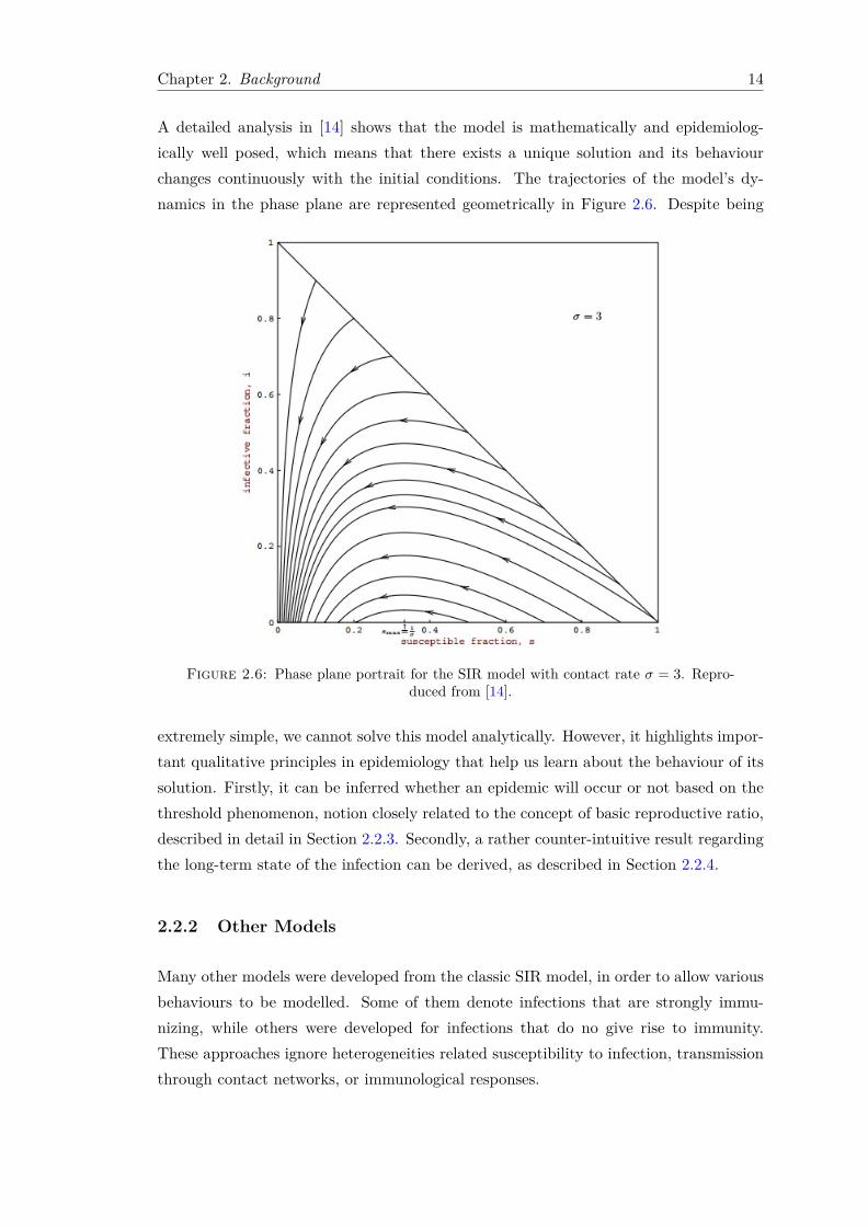
A detailed analysis in [14] shows that the model is mathematically and epidemiolog-ically well posed, which means that there exists a unique solution and its behaviourchanges continuously with the initial conditions. The trajectories of the model’s dy-namics in the phase plane are represented geometrically in Figure 2.6. Despite being
Figure 2.6: Phase plane portrait for the SIR model with contact rate σ = 3. Repro-duced from [14].
extremely simple, we cannot solve this model analytically. However, it highlights impor-tant qualitative principles in epidemiology that help us learn about the behaviour of itssolution. Firstly, it can be inferred whether an epidemic will occur or not based on thethreshold phenomenon, notion closely related to the concept of basic reproductive ratio,described in detail in Section 2.2.3. Secondly, a rather counter-intuitive result regardingthe long-term state of the infection can be derived, as described in Section 2.2.4.
2.2.2 Other Models
Many other models were developed from the classic SIR model, in order to allow variousbehaviours to be modelled. Some of them denote infections that are strongly immu-nizing, while others were developed for infections that do no give rise to immunity.These approaches ignore heterogeneities related susceptibility to infection, transmissionthrough contact networks, or immunological responses.
Chapter 2. Background 15
SI model The SI model was developed to account for the case when the infectioncan induce mortality. S and I remain the subpopulations of susceptibles and infected,respectively. We also consider ρ as the probability of an infected individual to die beforerecovery or from natural causes, which takes values between 0 and 1. Additionally, µis the rate of natural mortality. Mathematically, the model is described by the set ofODEs:
dS
dt= −βSI (2.7)
dI
dt= βSI − (γ + µ)
1− ρ I (2.8)
There are other variations to this model that take into account various stages at whichan infection may produce mortality.
SIS model The previous described models illustrate the dynamics of epidemics thateither confer immunity after recovery or induce death. The SIS model captures thoseepidemics that don’t confer life-lasting immunity, such that an individual recovered fromthe infection becomes susceptible again. The long term persistence is guaranteed by theloss of immunity, which always replenished the susceptibles pool. The following pair ofODEs describe the model:
dS
dt= γI − βIS (2.9)
dI
dt= βSI − γI (2.10)
The parameters remain similar to the ones in the previous section, except that S+I = N ,where N is the total size of the population.
SEIR model The SEIR model introduces a new category of individuals E, namelyExposed, consisting of individuals who are infected, but not yet infectious. Taking theaverage duration of this latent period is 1
α , the model is given by the following differentialequations:
dS
dt= −βSI (2.11)
dE
dt= βSI − αE (2.12)
dI
dt= αE − γI (2.13)
dR
dt= γI (2.14)
We also assume that S + E + I +R = N . Compared to the SIR model, it has a slowergrowth rate due to the fact that individuals must belong to the Exposed subpopulationbefore being able to transmit the infection.
Chapter 2. Background 16
MSEIR model A more general model is MSEIR, which also includes a categoryof individuals that are passively immune since their mothers developed some type ofimmunity. It is suitable for modelling a directly transmitted disease with permanentimmunity after recovery, in a population with variable total size. It translates to thefollowing system of differential equations:
dM
dt= b(N − S)− (δ + d)M (2.15)
dS
dt= bS + δM − βSI/N − dS (2.16)
dE
dt= βSI/N − (ε+ d)E (2.17)
dI
dt= εE − (γ + d)I (2.18)
dR
dt= (b− d)N (2.19)
where b and d are the constant rates of birth and death, respectively.
2.2.3 Basic Reproductive Ratio
For the SIR model, a famous result highlighted by Kermack and McKendrick [13] isknown in the literature as the threshold phenomenon. It states that in order for anepidemic to spread, the initial number of susceptibles must exceed a certain threshold,equal to γ/β. The value of the threshold is derived by re-writing Equation 2.2 as:
dI
dt= I(βS − γ) (2.20)
In the initial stage, after I(0) infected individuals are introduced in the population,the infection becomes extinct if dI/dt < 0, which is equivalent to S(0) < γ/β. Thisthreshold is referred to as the relative removal rate, which must be small enough inorder to allow the infection to spread.
The inverse of this rate is called basic reproductive ratio R0, and constitutes one of themost important measures in epidemiology. It is formally defined in [15] as:
the expected number of secondary infections arising from a single individual during hisor her entire infectious period, in a population of susceptibles .
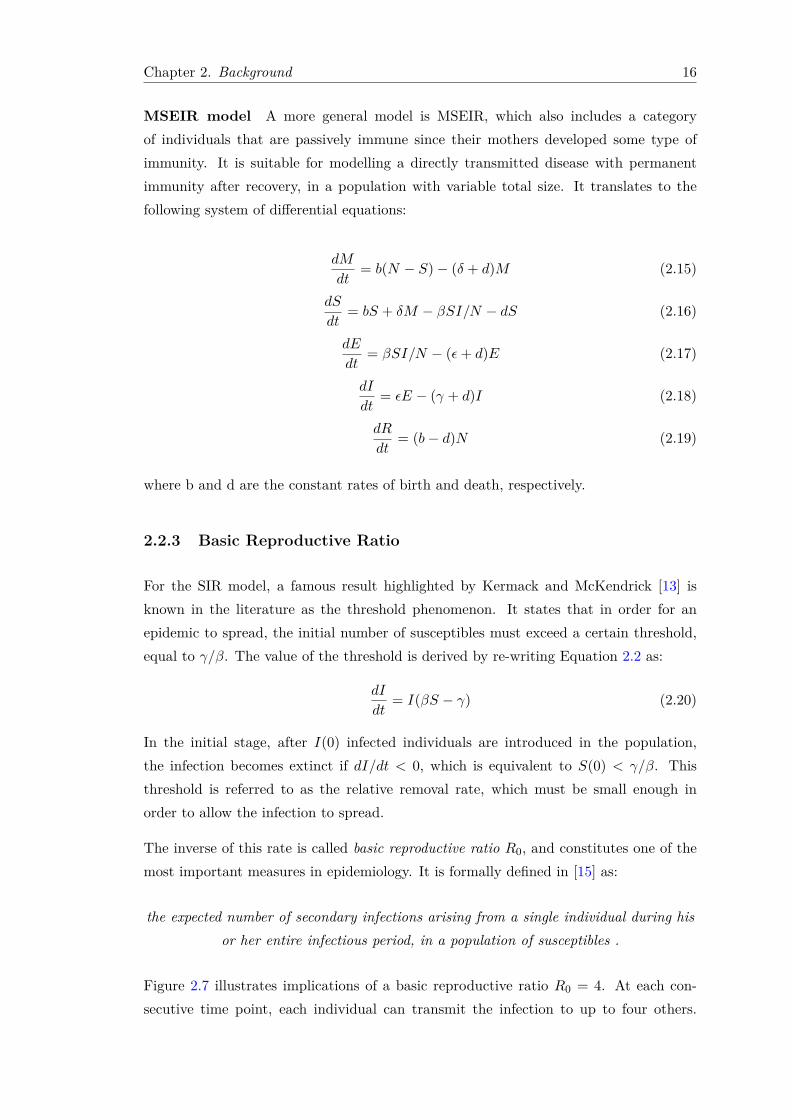
Figure 2.7 illustrates implications of a basic reproductive ratio R0 = 4. At each con-secutive time point, each individual can transmit the infection to up to four others.
Chapter 2. Background 17
Figure 2.7: Implications of a basic reproductive ratio R0 = 4.Reproduced from [12].
In an entirely susceptible population (a), the incidence increases exponentially. In apopulation that is 75% immune (b), only 25% of the contacts lead to infection.
From the definition, it follows immediately that an epidemic will spread if and onlyif R0 > 1, which is just another way of expressing the threshold phenomenon. In itssimplest form, R0 is mathematically expressed as:
R0 = β
γN = cpD (2.21)
whereβ = infection rateγ = recovery rateN = total size of the population
c = contact ratep = transmission probability given contactD = duration of infectiousness
However, estimating R0 from individual parameters is not always feasible, as they mightbe unknown or impossible to estimate. Alternatively, the basic reproductive ratio canbe estimated from epidemic time series data [16].
Chapter 2. Background 18
If the exponential growth rate of the initial phase r is available, then:
R0 = 1 + rD (2.22)
If the doubling time of the number of infected individuals td is known, then:
R0 = 1 + Dln2td
(2.23)
If we consider s0 the number of susceptibles before the outbreak and sα the number ofsusceptibles after the epidemic dies out, then:
R0 = ln(S0)− ln(sα)s0 − sα
(2.24)
Table 2.2 presents examples of various diseases and their corresponding estimated valuesfor the basic reproductive ratio. Because R0 depends on both the disease and the hostpopulations, differences in demographics or contact rates may lead to different estimatedvalues for the same disease.
Infectious disease Host Estimated R0 Reference
Rabies DogsKenya 1.1 - 1.5 Smith (2011)
Tuberculosis Cattle 2.6 Goodchild andClifton-Hadley (2001)
1918 PandemicInfluenza Humans 2 - 3 Mills et al. (2004)
Foot-and-mouthDisease
Livestock farmsUK 3.5 - 4.5 Ferguson et al. (2001)
Rubella HumansUK 10 - 12 Anderson and May (1991)
Measels HumansUK 16 - 18 Anderson and May (1982)
Table 2.2: Estimated basic reproductive ratios for various diseases. Adapted from[12].
2.2.4 Epidemic Burnout
Another important result derived from the SIR model is related to the long-term stateof the epidemic. Firstly, it has been observed that there will always be a certain numberof susceptible individuals who do not get infected. Mathematically, this can be derived
Chapter 2. Background 19
by dividing Equation 2.1 by Equation 2.3:
dS
dR= −βS
γ= −R0S (2.25)
and integrating with respect to R:
S(t) = S(0)e−R(t)R0 (2.26)
This shows that S always stays positive. The conclusion that emerges from this result israther counter-intuitive: the chain of transmission eventually breaks due to the declinein infectives, not due to a complete lack of susceptibles [10].
2.3 Uncertainty Sources
The application of compartmental models in epidemiological modelling is accompaniedby concerns regarding the degree of uncertainty prevailing in their use. There are twomain sources of uncertainty that we consider, discussed below.
2.3.1 Stochastic Uncertainty
Stochastic uncertainty arises from the randomness present in the evolution of an epi-demic. If an infectious disease outbreak would re-occur, we would not observe the exactsame number of infected individuals at the same time. This intuitively suggests that astochastic model is always desirable, being more realistic. However, the magnitude of thefluctuations depend on the population size. A large population reduces the fluctuationlevel, hence a deterministic model can provide a good approximation. When addressingsmall populations or diseases with reduced level of incidence, stochasticity can make atremendous difference. It introduces variances and co-variances that may lead to chanceextinction of the disease.
Computationally, stochastic uncertainty can be simulated using Gillespie’s discrete-eventsimulation algorithm (SSA) [17]. This is applicable to systems that can be modelled as acontinuous-time Markov process whose probability distribution obeys a so called “masterequation”. It produces single realisations of the stochastic process that statistically agreewith the master equation.
Chapter 2. Background 20
2.3.2 Parameter Uncertainty
Parameter uncertainty relates to the fact that the outcomes of fitting data against amodel are themselves uncertain, because they are quantities estimated from subjectiveinformation. Factors such as the sample size informing that estimate, and variance inthe data contribute to determining the level of parameter uncertainty.
2.4 Other Applications of Epidemiological Models
2.4.1 Social Network Analysis
Online Social Networks (OSN) represent web-based services that allow users to havea presence via their individual profile, build a list of connections and interact withthem. The concept originated in the 1960s with Plato, a computer-based education tooldeveloped at University of Illinois, but the viral growth and commercial interest presenttoday only started after the advent of the Internet. Nowadays, online social networkingis a mass adoption phenomenon. For example, public data on Facebook’s website, thelargest OSN at present, reveals 1.23 billion monthly active users, with an average of 757million users that log in daily as of December, 31 2013. Every 20 minutes, 1 million linksare being shared, 2 million friends requested and 3 million messages sent on average [6].
Social network analysis has a wide range of applications across multiple disciplines suchas data aggregation and mining, network modelling, user attribute and behaviour anal-ysis, location-based interaction, social sharing and filtering, recommendation systemsdevelopment, or link prediction. In the private sector, businesses use OSN analysis forto fulfil their marketing and business intelligence needs, while in the public sector itserves to the development of leader engagement and community-based problem solving.Also, law enforcement and intelligence institutions make use of this technique in fightingand preventing crime.
The relationships among social entities and the patterns and implications they have oncontent spreading developed researchers’ interest in OSN analysis. The online environ-ment promotes viral dissemination of information, creating powerful electronic world-of-mouth effects that result in the birth of online trends [8].
2.4.2 Economic cycles
The idea of adopting in economics tools and techniques from biology is not new, beingfirstly highlighted by the neoclassical economist Alfred Marshall in the preface to his
Chapter 2. Background 21
Principles of Economics (1890): “the Mecca of the economist lies in economic biology”.If we consider the economy as a heterogeneous system comprising of different typologiesof agents that interact, influence each other and have different levels of knowledge aboutthe environment and each other, then biology can provide the necessary tools to explainvarious behaviours of agents.
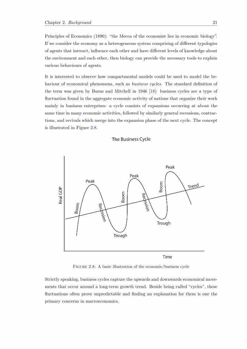
It is interested to observe how compartmental models could be used to model the be-haviour of economical phenomena, such as business cycles. The standard definition ofthe term was given by Burns and Mitchell in 1946 [18]: business cycles are a type offluctuation found in the aggregate economic activity of nations that organize their workmainly in business enterprises: a cycle consists of expansions occurring at about thesame time in many economic activities, followed by similarly general recessions, contrac-tions, and revivals which merge into the expansion phase of the next cycle. The conceptis illustrated in Figure 2.8.
Figure 2.8: A basic illustration of the economic/business cycle
Strictly speaking, business cycles capture the upwards and downwards economical move-ments that occur around a long-term growth trend. Beside being called “cycles”, thesefluctuations often prove unpredictable and finding an explanation for them is one theprimary concerns in macroeconomics.
Chapter 2. Background 22
In economic literature we cannot find many applications of compartmental models. Oneof the few existing works related to this subject belongs to the Nobel laureate GaryBecker, who divides the population into various subclasses and analyses the causes ofdeceleration of the flow from one category to another, without specifically using the word”compartment”. Another approach, closer to the epidemiological models, is the one ofAoki [19], who introduces the notion of clusters, conceptually similar to compartments.A big difference, however, is the stochastic approach taken, which significantly increasesthe complexity of the mathematical tools required. A direct application of compart-mental models in economy is studied in [20], by introducing a simple model describinghow the government could operate in order to reach a certain goal as cost-efficiently aspossible.
2.4.3 Retail Sales
Another less explored area where epidemic models could be applied is retail sales. Theawareness of a new product spreads among customers similar to how a disease spreadsfrom an individual to another. Epidemic models could take various factors into account,such as the impact of previous negative experiences with a product, and use the numberof early adopters to project peak sales or sales volume levels over time.
This subject is little explored in the literature, although we can see how compartmentalmodels could be constructed. For example, in the context of online retail sales, [21] sug-gests to assign all major products categories to one of three market share groups: high,medium or low penetration potential. This division should be based on the suitability ofthe product to the online medium and its historical online success to date. However, theauthors of the report do not build a set of ODEs, but derive a specific logistic growthfunction for each category.
2.4.4 Computer Viruses
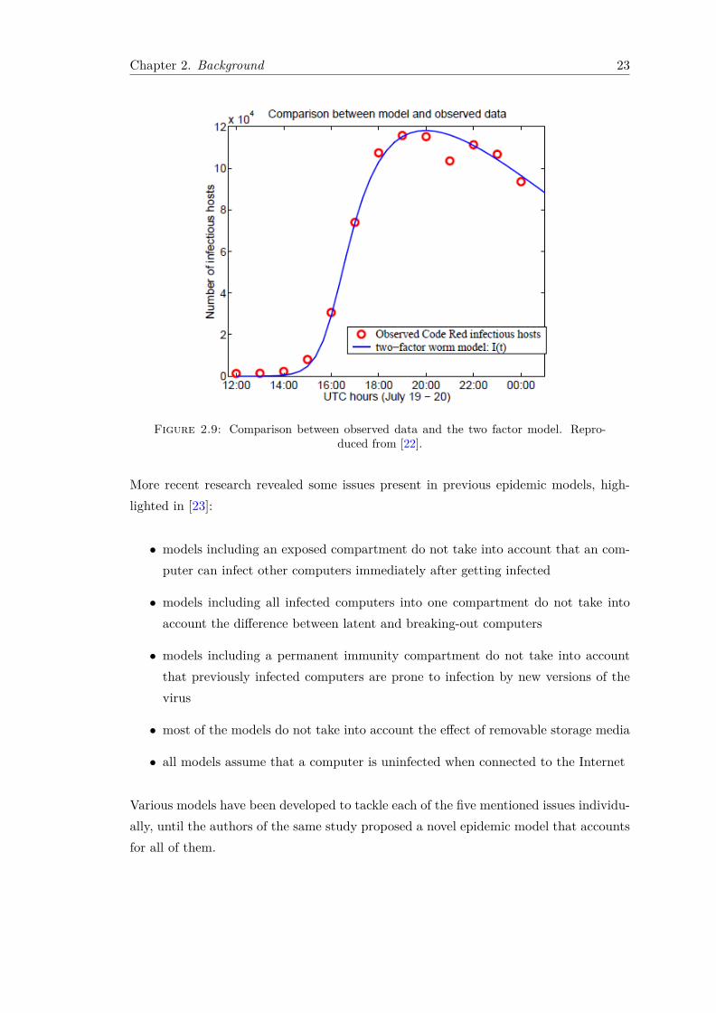
The Code Red worm incident that happened in July 2011 raised awareness regardingthe urge to build models for analysing how Internet viruses propagate. Researchersin [22] developed a general Internet worm model based on the classic epidemic SIRmodel, taking into account two major factors. Firstly, they considered the dynamiccountermeasures taken by users in removing susceptible and infectious computers. Thesecond factor taken into account is the slowed down infection rate, as a consequence ofthe congestions to some routers caused by its large-scale propagation. The results offitting the data for this model are illustrated in Figure 2.9.
Chapter 2. Background 23
Figure 2.9: Comparison between observed data and the two factor model. Repro-duced from [22].
More recent research revealed some issues present in previous epidemic models, high-lighted in [23]:
• models including an exposed compartment do not take into account that an com-puter can infect other computers immediately after getting infected
• models including all infected computers into one compartment do not take intoaccount the difference between latent and breaking-out computers
• models including a permanent immunity compartment do not take into accountthat previously infected computers are prone to infection by new versions of thevirus
• most of the models do not take into account the effect of removable storage media
• all models assume that a computer is uninfected when connected to the Internet
Various models have been developed to tackle each of the five mentioned issues individu-ally, until the authors of the same study proposed a novel epidemic model that accountsfor all of them.

Chapter 2. Background 24
2.5 Development Environment
2.5.1 Programming Language
In terms of programming language, the obvious choices were Matlab and R, both beingpowerful and widely used for statistical modelling and data analysis. With no experiencein either of the two languages, R was chosen after comparing their advantages anddisadvantages.
The main difference between the two comes from the fact that Matlab is a commercialsoftware, while R is open source. Therefore, R is free, allowing anyone to use it andcontribute to its enhancement. Its vast user community of over 2 million people isconstantly adding new packages, enriching its set of functionalities. At present, it is themost comprehensive statistical analysis tool available, making it ideally suited for thepurpose of this project. Statisticians were the ones who created R. This constitutes amajor advantage because it means data analysis lies at the very heart of the language.However, it is not as well documented as Matlab, and although many introductorytutorials are available, none of them are comprehensive enough. It is not straightforwardto obtain a clear overview of the available functionalities, and looking for the rightpackage can be time consuming.
R admittedly has a steep learning curve. Apart from the poor documentation, imple-mentation details, such as silent coercion or sometimes misleading textual presentationof objects contribute to this phenomenon. Mistakes are very easily made and carefulconsideration must be given in order to avoid common pitfalls. Despite this aspect, Rwas still preferable over Matlab due to its data frames. A data frame is a core datastructure, similar to a matrix in Matlab, with two primary advantages: firstly, the rowsand columns can be named rather than being referred by index, and secondly, eachcolumn can hold a different data type.
Similar to Matlab, R is cross-platform compatible, being available under various op-erating systems and architectures. It also integrates well with many other tools. Forexample, it can import data from sources such as CSV, Microsoft Excel, MySQL. It canalso produce graphics output in PDF, JPG, PNG, and SVG formats, and table outputfor LATEX and HTML. Compared to Matlab, that can produce high quality interac-tive plots, R’s visualisation capabilities are better suited for exploratory analysis, whichplays a major role in this project.
One of the main disadvantages of R concerns memory management. R holds objects invirtual memory, and limits are imposed on the amount of memory that can be used.The limitations apply to the size of the heap and the number of cons cells allowed.

Chapter 2. Background 25
The environment may further limit the user address space of a single process and theresources available to a single process. Because many R commands give little thought tomemory management, it can quickly run out of resources. However, this usually happenswhen working with huge data sets, which is beyond the scope of this project.
In terms of performance, both R and Matlab are fast when it comes to mathematicaloperations on arrays, which are the main data structures used throughout the project.However, they have slow language interpreters, discouraging complex abstractions.
Another possible choice would have been Python, which is overall a better programminglanguage than both R and Matlab. Its object oriented and functional nature, togetherwith libraries such as Numpy, Scipy, statsmodels, and matlibplot make it a powerfulstatistical tool. However, it lacks a strong community of mathematicians, so many ofthe functionalities already existing in Matlab and R are not yet available.
2.5.2 Additional Libraries and Tools
R: The main R packages used in this project are: deSolve, bbmle, and GillespieSSA.
The package deSolve provides general solvers for initial value problems of first orderOrdinary Differential Equations (ODEs) systems, assuming a full or banded Jacobianmatrix. It also includes fixed and adaptive time-step Runge-Kutta solvers, as well asthe Euler method.
The package bbmle provides tools for general maximum likelihood estimations. It ex-tends the stats4 default package, being superior to it in some respects. Firstly, thefunctions are more robust, with additional warnings that allow certain computations toreturn, rather than stop with an error. Secondly, it allows for more parameters to bepassed to the negative log-likelihood function via a data argument. Additionally, forsimple models an in-line formula may be passed to the optimisation procedure, insteadof defining a separate negative log-likelihood function.
The package GillespieSSA provides an interface to various stochastic simulation algo-rithms for generating simulated trajectories of finite population continuous-time models.The interface is simple to use, intuitive and easily extensible. Currently, it implementsvarious Monte Carlo procedures for Gillspie’s Stochastic Simulation Algorithm (SSA),including both direct and approximate methods.
Matlab: Although the main implementation language was chosen to be R, it proveda challenging environment for neat 3D surface plots. Hence, we used Matlab to produceisosurface plots.
Chapter 3
Fitting Procedure using LeastSquares
This chapter describes a least-squares-based epidemic fitting procedure of an SIR model,as the outbreak unfolds over time. We first introduce the basic idea behind this method.Then, we describe the model used for fitting, and provide mathematical details regardingthe objective function and the optimisation technique. Finally, we outline a measure toassess the goodness of fit. Our methodology tackles the challenge of considering theinitial number of susceptibles unknown.
Least Squares (LS) is a simple approach to investigate the evolution of epidemic dynam-ics over time and estimate the parameters values, first documented by Gauss around1794. We assume that the only source of variability in the data comes from measure-ment errors and that its variance is constant, with a symmetrical distribution. Underthese circumstances, Least Squares constitutes a statistically appropriate method for es-timation, being a procedure that allows finding approximate solutions of overdeterminedsystems, i.e. systems that have more equations than unknowns. The basic idea behindit is to test different values of parameters in order to find the best fit model for the givendata set. However, the robustness of least squares is highly dependent on how close tothe model are the data points. Thus, outliers can cause inaccurate estimates.
3.1 Model
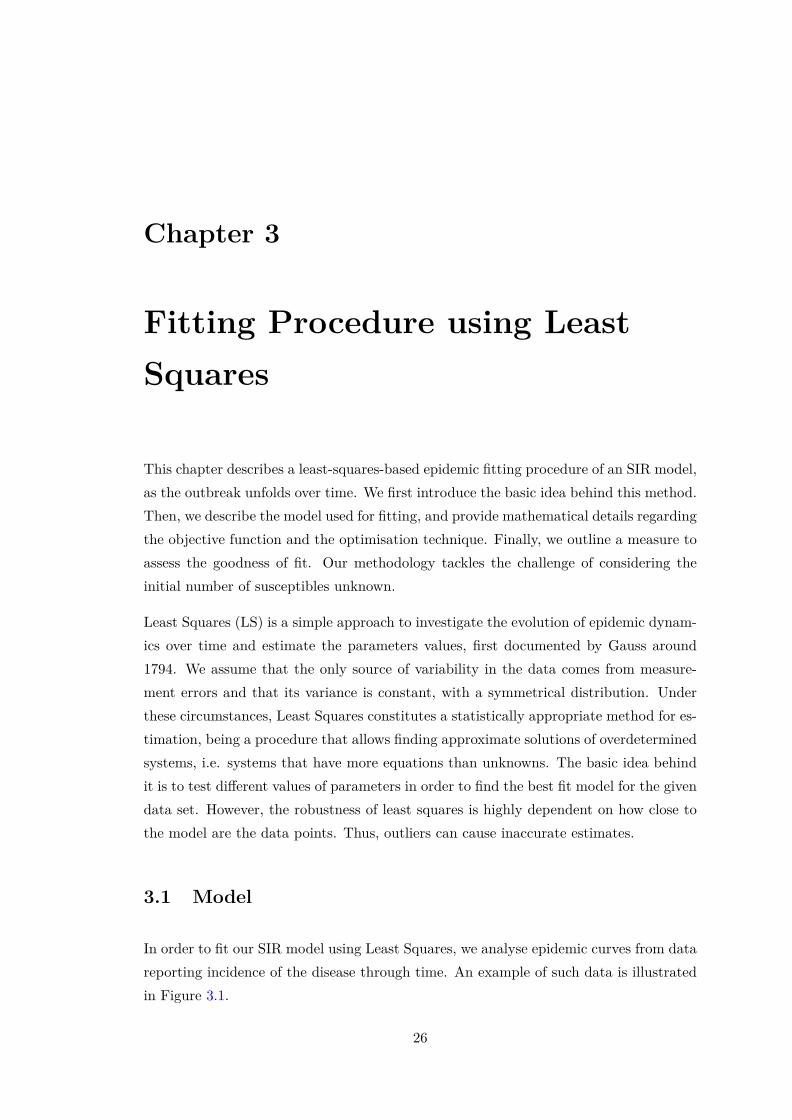
In order to fit our SIR model using Least Squares, we analyse epidemic curves from datareporting incidence of the disease through time. An example of such data is illustratedin Figure 3.1.
26
Chapter 3. LS Fitting Procedure 27
Figure 3.1: Daily number of infected individuals over a period of 100 days.
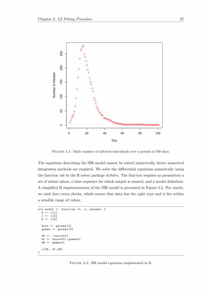
The equations describing the SIR model cannot be solved analytically, hence numericalintegration methods are required. We solve the differential equations numerically usingthe function ode in the R solver package deSolve. The function requires as parameters aset of initial values, a time sequence for which output is wanted, and a model definition.A simplified R implementation of the SIR model is presented in Figure 3.2. For clarity,we omit here extra checks, which ensure that data has the right type and it lies withina sensible range of values.
sir. model <- function (t, x, params ) {S <- x[1]I <- x[2]R <- x[3]
beta <- params [1]gamma <- params [2]
dS <- -beta*S*IdI <- beta*S*I- gamma *IdR <- gamma *I
c(dS , dI ,dR)}
Figure 3.2: SIR model equations implemented in R.
Chapter 3. LS Fitting Procedure 28
As integration method we use the integrator lsoda provided in the same package. Thissolver is robust due to its automatic detection of stiffness, i.e. property that makes un-stable certain numerical methods for solving equations, unless an extremely small stepsize is being used. Its implementation uses linear multi-step methods that approximatethe derivative of a given function using information computed in previous steps. Inparticular, an explicit multi-step Adams method is applied for non-stiff systems, andthe Backward Differentiation Formulas (BDF) method for the stiff ones. In terms ofaccuracy, the default relative tolerance and absolute tolerance are equal to 10−6, deter-mining the error control performed by the solver. Alternatively, a maximum value forthe integration step-size may be specified.
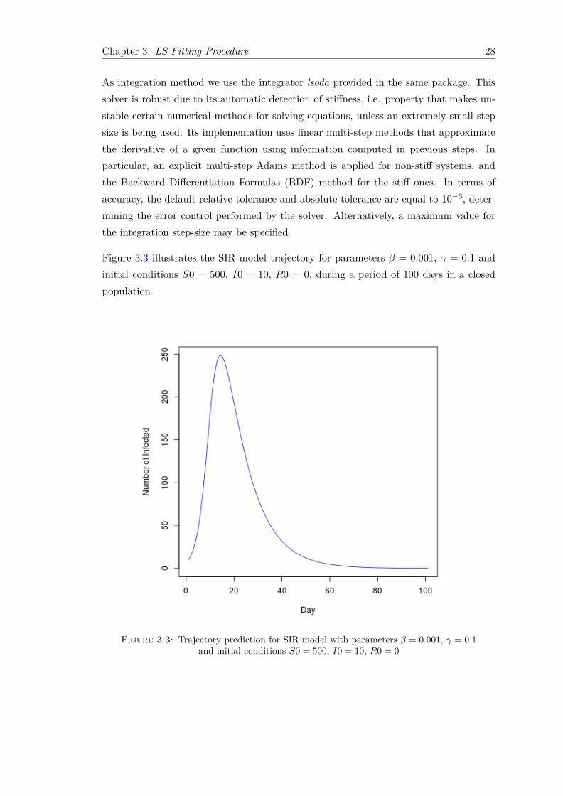
Figure 3.3 illustrates the SIR model trajectory for parameters β = 0.001, γ = 0.1 andinitial conditions S0 = 500, I0 = 10, R0 = 0, during a period of 100 days in a closedpopulation.
Figure 3.3: Trajectory prediction for SIR model with parameters β = 0.001, γ = 0.1and initial conditions S0 = 500, I0 = 10, R0 = 0
Chapter 3. LS Fitting Procedure 29
3.2 Objective Function
The first step in trajectory matching is defining an objective function. Least Squaresfinds a solution by minimising the sum of the squares of the errors. This is also oneof its limitations. Using the squares of the error differences in the presence of outlyingpoints may lead to a disproportionate effect in the fit, property which is usually notdesirable. Outliers can potentially cause the estimates to be outside a desired range ofaccuracy. The method is therefore only as robust as the observed data points are closeto the model.
The basic idea is to find estimates of the parameters that minimise the squared offsetsof the model predictions from the observed data. Algebraically, this is equivalent tominimising:
S =∑
(yi − f(xi, θ))2 (3.1)
where yi is the observed value, and f(xi, θ) is the model function, with θ being the vectorof unknown parameters.
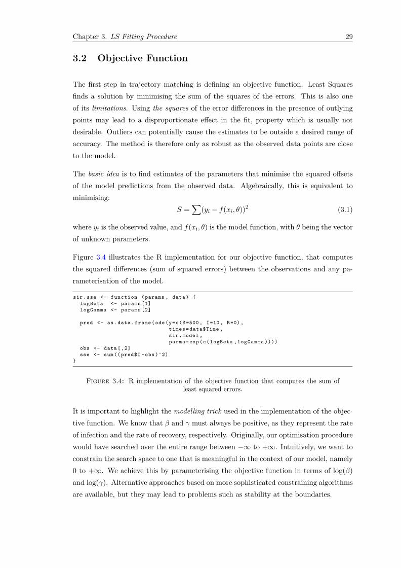
Figure 3.4 illustrates the R implementation for our objective function, that computesthe squared differences (sum of squared errors) between the observations and any pa-rameterisation of the model.
sir.sse <- function (params , data) {logBeta <- params [1]logGamma <- params [2]
pred <- as.data. frame (ode(y=c(S=500 , I=10 , R=0) ,times =data$Time ,sir.model ,parms =exp(c(logBeta , logGamma ))))
obs <- data [ ,2]sse <- sum (( pred$I -obs )ˆ2)
}
Figure 3.4: R implementation of the objective function that computes the sum ofleast squared errors.
It is important to highlight the modelling trick used in the implementation of the objec-tive function. We know that β and γ must always be positive, as they represent the rateof infection and the rate of recovery, respectively. Originally, our optimisation procedurewould have searched over the entire range between −∞ to +∞. Intuitively, we want toconstrain the search space to one that is meaningful in the context of our model, namely0 to +∞. We achieve this by parameterising the objective function in terms of log(β)and log(γ). Alternative approaches based on more sophisticated constraining algorithmsare available, but they may lead to problems such as stability at the boundaries.
Chapter 3. LS Fitting Procedure 30
3.3 Optimisation Technique
The second step computes the parameter estimates that minimise the objective function.To achieve this, we use the function optim in the R package stats, which provides robustalgorithms for general-purpose optimisations. The technique we selected is based onthe Nelder-Mead algorithm, a widely used method in multidimensional unconstrainedoptimisation. It falls under the general class of direct search methods, as it does notinvolve any explicit or implicit derivative information. This makes it suitable to solveoptimisation problems even when the objective function is not smooth [24].
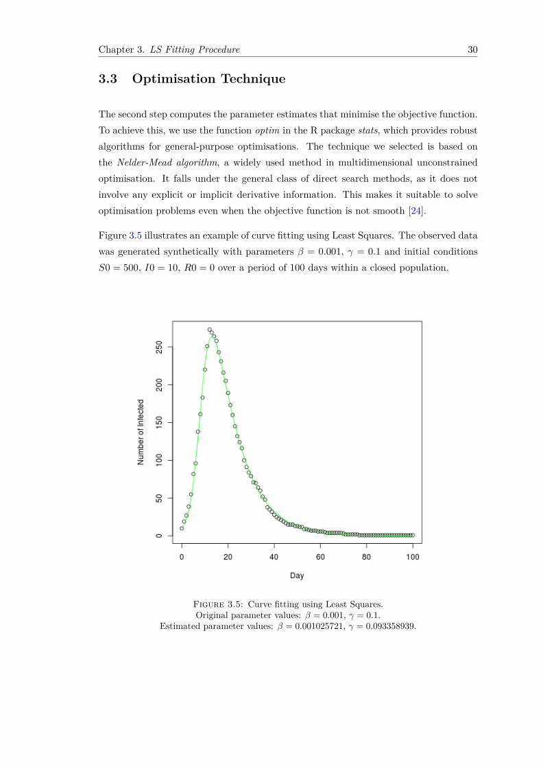
Figure 3.5 illustrates an example of curve fitting using Least Squares. The observed datawas generated synthetically with parameters β = 0.001, γ = 0.1 and initial conditionsS0 = 500, I0 = 10, R0 = 0 over a period of 100 days within a closed population.
Figure 3.5: Curve fitting using Least Squares.Original parameter values: β = 0.001, γ = 0.1.
Estimated parameter values: β = 0.001025721, γ = 0.093358939.
Chapter 3. LS Fitting Procedure 31
3.4 Goodness of Fit
Finally, after fitting the data with the model, we evaluate the goodness of fit. We aimto assess how well a chosen set of parameters fits the observed data by identifying thediscrepancies between them. After a visual examination, we make use of the coefficientof determination, denoted R2.
R2 is a statistical measure, usually reported in the context of regression. It determineshow much of the total variation present in the observed data is explained by the model.The sample variance is proportional to the total sum of squares SStot, given by Equation3.2. To measure how far from the observed data are the estimates, we compute theresidual sum of squares SSres, using Equation 3.3.
SStot =∑i
(yi − y)2 (3.2)
SSres =∑i
(yi − fi)2 (3.3)
where fi are the model predictions, yi are the observed data points and y is the meanof the observed data, given by Equation 3.4.
y = 1n
n∑i=1
yi (3.4)
Based on these measures, the coefficient of determination is defined by Equation 3.5:
R2 = 1− SSresSStot
(3.5)
Generally, R2 ranges between 0 and 1. Its interpretation denotes the degree of improve-ment the model has made over the average of the observed data. Hence, the closer R2
is to 0, the least agreement between the actual and estimated values is observed. Thecloser R2 is to 1, the better explained is the variability in the data. However, from thedefinition we notice that R2 can take negative values if SSres > SStot. In this situation,it can be inferred that the mean of the observed data provides better estimates than theones of the fitted model. A key limitation of R2 is that it cannot determine whetherthe model prediction and estimates are biased. This is why we must also examine theresidual plots.
Chapter 4
Uncertainty Characterisationusing Maximum Likelihood
This chapter describes a new maximum-likelihood-based epidemic fitting procedure ofSIR model as the outbreak unfolds over time, yielding confidence intervals on the esti-mated parameters. It is a generic, fully-automated methodology for rigorous character-isation of the uncertainty inherent in the estimated values. We first introduce the basicidea behind Maximum Likelihood, providing mathematical details about the objectivefunction and the optimisation technique used. Then, we discuss how confidence intervalscharacterise uncertainty. Finally, we present step-by-step the new methodology and givea three-dimensional visualisation of the confidence intervals. We tackle the challenges ofestimating parameters when the initial number of susceptibles and infected is unknown.
Maximum Likelihood (ML) is one of the most versatile analytic procedures for fittingstatistical models to data, dating back to early works of Fisher around 1925. Typically,it finds parameter estimates that maximise the likelihood of a given dataset. Thereare many advantages of using likelihood-based approaches. Firstly, they are flexible,being applicable to a wide range of statistical models and various type of data sets (i.e.discrete, continuous, truncated, categorical, etc). Secondly, not only can they estimateparameters values, but also provide confidence intervals to characterise the uncertaintyinherent in these estimates, due to their asymptotic normality propriety. Finally, theycan be regarded as a unifying framework, as many common statistical approaches repre-sent special cases of them. For example, Least Squares fitting is equivalent to MaximumLikelihood when the errors are normally distributed. To summarise, Maximum Likeli-hood based approaches are considered to be more robust, have better sufficiency andsmaller errors than other methods.
32
Chapter 4. ML Uncertainty Characterisation 33
4.1 Objective Function
Similar to Least Squares, the first step is defining an objective function. MaximumLikelihood finds a solution by maximising a likelihood function, defined as the probabilityof a given dataset having occurred, given a particular hypothesis. This is algebraicallyequivalent to Equation 4.1:
L(D|H) = P(D|H) (4.1)
where D represents the observed data set and H is the hypothesis to be tested.
More precisely, the likelihood function is characterised by Equation 4.2.
L(θ |x1, . . . , xn) = f(x1, x2, . . . , xn|θ) =n∏i=1
f(xi|θ) (4.2)
where xi are the observed data points, θ is the vector of unknown parameters and f(xi, θ)is the associated probability density function.
However, it is usually computationally more convenient to make use of the naturallogarithm of the likelihood function, referred to as the log likelihood. Mathematically,this is defined in Equation 4.3.
logL(θ |x1, . . . , xn) =n∑i=1
log f(xi|θ) (4.3)
where xi are the observed data points, θ is the vector of unknown parameters and f(xi|θ)is the associated probability density function, as before.
This substitution is possible due to the increasing monotonicity of the logarithm func-tion. This property makes both the logarithm function and the function itself achieve themaximum value at the same points. There are two main computational advantages ofusing the logarithm of the function. Firstly, the natural logarithm reduces the potentialfor underflow that may be caused by very small likelihoods. The second advantage ariseswhen computing the derivative of the function, which is required to find its maximum.The likelihood function factorises into a product of functions, as shown in Equation 4.2,because the observed data points are assumed to be independent of each other. However,the logarithm of this product becomes a sum of individual functions in Equation 4.3,which is considerably easier to differentiate than a product.
In our implementation, we minimise the negative log likelihood function instead, as de-fined by Equation 4.4, which is just an equivalent characterisation.
neg logL(θ |x1, . . . , xn) = −n∑i=1
log f(xi|θ) (4.4)
Chapter 4. ML Uncertainty Characterisation 34
Based on the observation in Equation 4.5,
argmaxx
(x) = argminx
(−x) (4.5)
the equivalence in Equation 4.6 holds.
argmaxx
n∑i=1
log f(xi|θ) = argminx
(−n∑i=1
log f(xi|θ)) (4.6)
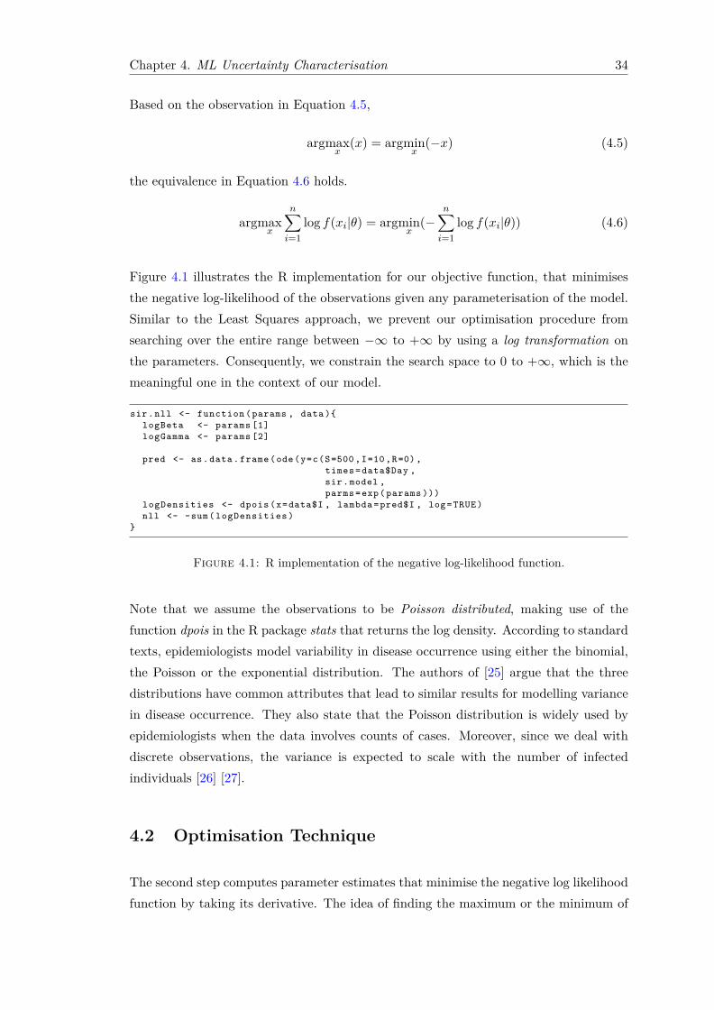
Figure 4.1 illustrates the R implementation for our objective function, that minimisesthe negative log-likelihood of the observations given any parameterisation of the model.Similar to the Least Squares approach, we prevent our optimisation procedure fromsearching over the entire range between −∞ to +∞ by using a log transformation onthe parameters. Consequently, we constrain the search space to 0 to +∞, which is themeaningful one in the context of our model.
sir.nll <- function (params , data ){logBeta <- params [1]logGamma <- params [2]
pred <- as.data. frame (ode(y=c(S=500 ,I=10 ,R=0) ,times =data$Day ,sir.model ,parms =exp( params )))
logDensities <- dpois (x=data$I , lambda =pred$I , log=TRUE)nll <- -sum( logDensities )
}
Figure 4.1: R implementation of the negative log-likelihood function.
Note that we assume the observations to be Poisson distributed, making use of thefunction dpois in the R package stats that returns the log density. According to standardtexts, epidemiologists model variability in disease occurrence using either the binomial,the Poisson or the exponential distribution. The authors of [25] argue that the threedistributions have common attributes that lead to similar results for modelling variancein disease occurrence. They also state that the Poisson distribution is widely used byepidemiologists when the data involves counts of cases. Moreover, since we deal withdiscrete observations, the variance is expected to scale with the number of infectedindividuals [26] [27].
4.2 Optimisation Technique
The second step computes parameter estimates that minimise the negative log likelihoodfunction by taking its derivative. The idea of finding the maximum or the minimum of
Chapter 4. ML Uncertainty Characterisation 35
a function by taking its derivative is based on the extreme value theorem. This statesthat if a function f(x) is continuous on a closed interval [a, b], then f(x) has a maximumand minimum value on the interval [a, b]. Algebraically, there exist xmin and xmax suchthat the formula in Equation 4.7 holds.
f(xmin) ≤ f(x) ≤ f(xmax), ∀x ∈ [a, b] (4.7)
Besides this theorem, there are two additional observations to be made. Firstly, the slopeof the tangent line of the maximum and minimum is 0. Secondly, after the maximumthe function decreases, and after the minimum it increases in value. Hence, the followingtwo conditions must be met by xmax in order for it to be a maximum of a function f:f ′(xmax) = 0 and f ′′(xmax) < 0. Similarly, xmin must meet the following two conditionsin order to be a minimum of a function f: f ′(xmin) = 0 and f ′′(xmin) > 0.
For multiple unknown parameters θi, finding Maximum Likelihood based estimates be-comes more challenging. The estimation requires determining the simultaneous solutionset for k equations, where k in the number of unknowns. Particularly, for the negativelog likelihood function neg logL and k = 2, the system is shown in Equation 4.8.
∂neg logL(θ1,θ2)∂θ1
= 0∂neg logL(θ1,θ2)
∂θ2= 0
(4.8)
In our implementation, we achieve this through the mle2 function in the bbmle R pack-age, which provides tools for general maximum likelihood estimation. This function usesthe same optimiser that we used for Least Squares, optim from the stats package, whichis based on the Nelder-Mead algorithm. It also computes an approximate covariancematrix for the parameters by inverting the Hessian matrix at the optimum, which canbe later used to derive confidence intervals.
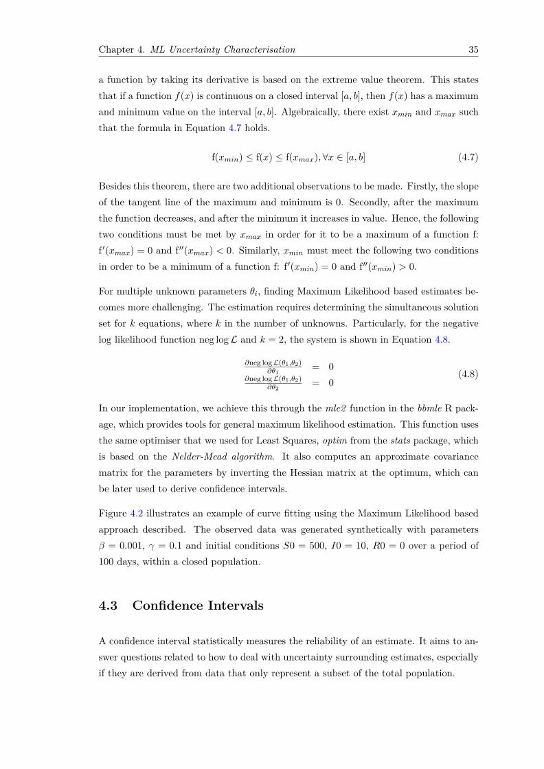
Figure 4.2 illustrates an example of curve fitting using the Maximum Likelihood basedapproach described. The observed data was generated synthetically with parametersβ = 0.001, γ = 0.1 and initial conditions S0 = 500, I0 = 10, R0 = 0 over a period of100 days, within a closed population.
4.3 Confidence Intervals
A confidence interval statistically measures the reliability of an estimate. It aims to an-swer questions related to how to deal with uncertainty surrounding estimates, especiallyif they are derived from data that only represent a subset of the total population.
Chapter 4. ML Uncertainty Characterisation 36
Figure 4.2: Curve fitting using Maximum Likelihood.Original parameter values: β = 0.001, γ = 0.1.
Estimated parameter values: β = 0.001034596, γ = 0.092604365.
The interpretation of a confidence intervals is not strictly a mathematical issue, but alsoa philosophical matter [28]. Mathematics has only a limited role in deciding why anapproach is preferred to another. Generally, there are multiple interpretations that canbe given to a confidence interval. For the purpose of our work, we will consider the caseexpressed in terms of repeated samples. The 95% confidence interval will ideally containthe true value of the parameter 95% of the time, given repeated fittings of the model. Itis only by chance that the true value of the parameter lies outside the confidence intervalwith probability 5%.
Traditionally, the Wald-type confidence intervals are widely used as an approximationto profile intervals. The standard procedure for computing such a confidence interval isby applying Equation 4.9.
estimate± (percentile × SE(estimate)) (4.9)
where SE is the standard error and the percentile is selected according to the desired con-fidence level and a reference distribution, i.e. a t-distribution for regression coefficientsin a linear model, otherwise a standard normal distribution.
They are easier to compute for complex models, but perform poorly when the likelihood
Chapter 4. ML Uncertainty Characterisation 37
surface is not quadratic. Additionally, a markedly skewed distribution of the parameterestimator or a standard error that poorly approximates the standard deviation of theestimator may affect their performance. Moreover, for generalised linear models, thestandard errors are based on asymptotic variance derived from the covariance matrix.For small to medium sample sizes, this scenario may also cause poor performance.
Profile likelihood confidence intervals represent a more robust approach [29]. They donot assume normality of the estimator and appear to perform better for small samplessizes than Wald-type confidence intervals. These confidence intervals are based on anasymptotic approximation of the χ2 distribution of the log-likelihood ratio statistic. Todefine them, we consider a model with θ the parameter of interest and δ a vector ofthe other parameters, and a likelihood function L(θ, δ). Then, the profile likelihoodfunction for θ, L1 is given by Equation 4.10. By definition, the profile likelihood equalsthe maximum value of the likelihood function for every point.
L1(θ) = maxδL(θ, δ) (4.10)
The 100(1− α) profile confidence interval is computed by inverting the likelihood ratiotest. Mathematically speaking, given a parameter θ, it contains the set of all values θ0
that do not reject the two-sided test of the null hypothesis H0 : θ = θ0 at a level ofsignificance α. The likelihood ratio test statistic of the hypothesis is defined by:
D = 2 [logL(θ, δ)− logL1(θ0)] (4.11)
Based on the asymptotic χ2 distribution of the likelihood ratio test statistic, if the nullhypothesis is true, the test of H0 : θ = θ0 will not be rejected at the level of significanceα if and only if the relation in Equation 4.12 holds.
D ≤ χ21−α (4.12)
where χ21−α is the (1− α) quantile of the χ2 distribution on 1 degree of freedom.
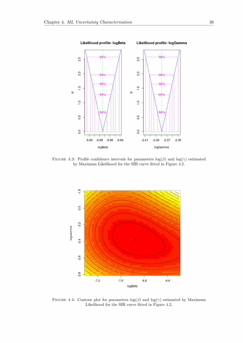
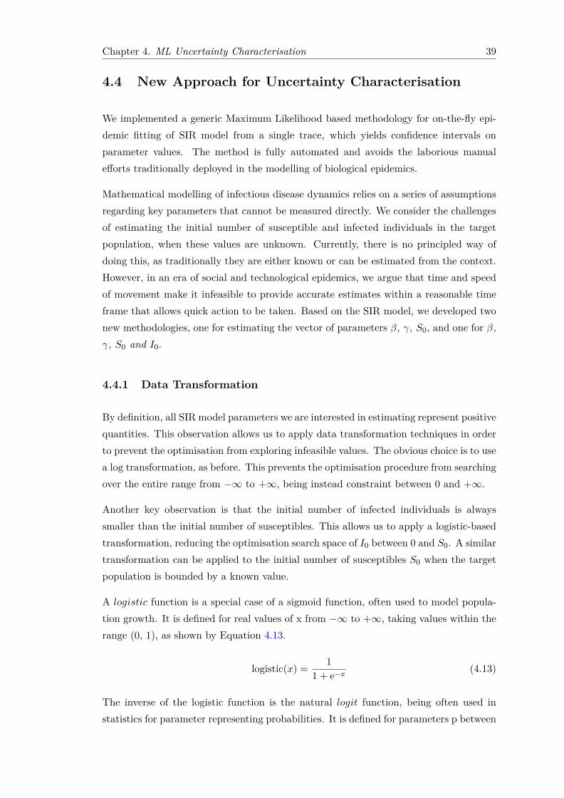
We compute two sided confidence intervals using the confint function in the bbmle Rpackage, as illustrated in Figure 4.3. Figure 4.4 is its corresponding two-dimensionalcontour plot, generated using function curve3d in the R package emdbook, and contour,points in the package graphics.
Chapter 4. ML Uncertainty Characterisation 38
Figure 4.3: Profile confidence intervals for parameters log(β) and log(γ) estimatedby Maximum Likelihood for the SIR curve fitted in Figure 4.2.
Figure 4.4: Contour plot for parameters log(β) and log(γ) estimated by MaximumLikelihood for the SIR curve fitted in Figure 4.2.
Chapter 4. ML Uncertainty Characterisation 39
4.4 New Approach for Uncertainty Characterisation
We implemented a generic Maximum Likelihood based methodology for on-the-fly epi-demic fitting of SIR model from a single trace, which yields confidence intervals onparameter values. The method is fully automated and avoids the laborious manualefforts traditionally deployed in the modelling of biological epidemics.
Mathematical modelling of infectious disease dynamics relies on a series of assumptionsregarding key parameters that cannot be measured directly. We consider the challengesof estimating the initial number of susceptible and infected individuals in the targetpopulation, when these values are unknown. Currently, there is no principled way ofdoing this, as traditionally they are either known or can be estimated from the context.However, in an era of social and technological epidemics, we argue that time and speedof movement make it infeasible to provide accurate estimates within a reasonable timeframe that allows quick action to be taken. Based on the SIR model, we developed twonew methodologies, one for estimating the vector of parameters β, γ, S0, and one for β,γ, S0 and I0.
4.4.1 Data Transformation
By definition, all SIR model parameters we are interested in estimating represent positivequantities. This observation allows us to apply data transformation techniques in orderto prevent the optimisation from exploring infeasible values. The obvious choice is to usea log transformation, as before. This prevents the optimisation procedure from searchingover the entire range from −∞ to +∞, being instead constraint between 0 and +∞.
Another key observation is that the initial number of infected individuals is alwayssmaller than the initial number of susceptibles. This allows us to apply a logistic-basedtransformation, reducing the optimisation search space of I0 between 0 and S0. A similartransformation can be applied to the initial number of susceptibles S0 when the targetpopulation is bounded by a known value.
A logistic function is a special case of a sigmoid function, often used to model popula-tion growth. It is defined for real values of x from −∞ to +∞, taking values within therange (0, 1), as shown by Equation 4.13.
logistic(x) = 11 + e−x (4.13)
The inverse of the logistic function is the natural logit function, being often used instatistics for parameter representing probabilities. It is defined for parameters p between
Chapter 4. ML Uncertainty Characterisation 40
0 and 1, and takes values from −∞ to +∞, as shown in Equation 4.14.
logit(p) = log( p
1− p) (4.14)
We modify the logistic function and its inverse in order to map the searching spaceranging from −∞ to +∞ to one between 0 and maxV alue, where maxV alue representseither the number of initial susceptibles, or the population bound, as discussed above.Hence, the transformation function is given by Equation 4.15
trans(x) = maxV al
1 + e−x(4.15)
and its corresponding inverse is defined in Equation 4.16.
untrans(y) = log( y
maxV al − y) (4.16)
4.4.2 Parameter Space Searching
To account for uncertainty as each outbreak unfolds over time, we apply our fittingmethodology on truncated data sets. For each dataset, we initially consider the first 3observations. Then, we add one observation at a time, until we reach the end of theoutbreak, creating new truncated datasets each time.
We compute parameters estimations for each truncated dataset, considering in turn eachof the following vectors of unknown parameters: β, γ, S0 and β, γ, S0, I0. The processof searching the parameter space for each set of parameters takes place in two stages.First, we find the parameters estimates that give the best fit to the data based on a LeastSquares objective function. In order to avoid the optimisation procedure being trappedin a local minimum, we restart for 20 different randomly chosen initial values of theparameter vectors. Sensible restrictions are imposed, such as 0 < β < γ and 0 < I0 < S0.The final candidate is selected to be the vector that yields the lowest value for the initialnumber of susceptibles S0 across all runs. Then, we use the parameter estimates obtainedin the first stage as initial values for a Maximum Likelihood fitting procedure. The reasonbehind this approach is to overcome computational challenges that arises through theestimation and confidence interval calculation within the mle2 function in the R packagebbmle. Maximum Likelihood based approaches are considerably more sensitive to theinitial guesses of the parameters to be estimated than the Least Square ones. If theseguesses are not within a sensible range, being too far off the true values, then the outputbecomes unreliable. Moreover, computing the confidence intervals using mle2 involves
Chapter 4. ML Uncertainty Characterisation 41
calculating the covariance matrix for the parameters, which is done by inversion of theHessian matrix at the optimum. This procedure can also be unsuccessful depending onthe initial parameters.
4.4.3 Visualisation
Once the fitting procedure completes successfully, we provide a three-dimensional vi-sualisation of the confidence intervals when the vector of unknown estimates is β, γ,S0. It expands on the idea of a two-dimensional contour plot previously explored inthe literature, where each contour line connects values that lie within the same confi-dence interval. We take this approach one step further and add more dimensions. Theresulting representation is therefore based on isosurfaces, the three-dimensional analogof isolines. Each of the surfaces represent parameters values that lie in the same confi-dence interval within a volume of space. Their shape is a variation of an ellipsoid. Thethree unequal axes represent the size of the confidence intervals corresponding to eachof the three parameters. These intervals may be asymmetrical, hence the surfaces aredescribed by a modified version of the ellipsoid’s in Equation 4.17. Higher dimensionalanalog representation require more complicated equations and are difficult to visualise,hence are not discussed further.
(x− x0)2
a1a2+ (y − y0)2
b1b2+ (z − z0)2
c1c2= 1 (4.17)
where x0, y0, z0 are the coordinates of the origin - the true values in our case, and ai,bi, ci are the corresponding confidence intervals sizes.
The isosurface plots were generated in Matlab. A sample example is illustrated inFigure 4.5. It clearly indicates that the estimated range of possible values is wider asthe confidence level increase.
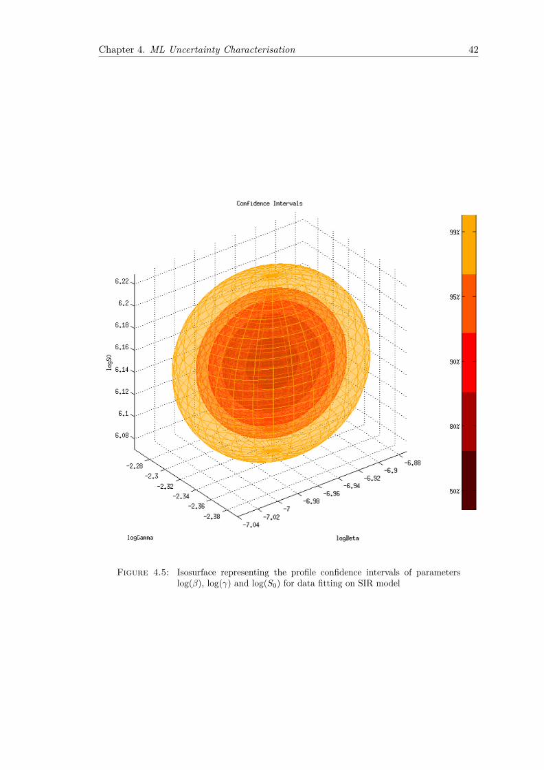
Chapter 4. ML Uncertainty Characterisation 42
Figure 4.5: Isosurface representing the profile confidence intervals of parameterslog(β), log(γ) and log(S0) for data fitting on SIR model
Chapter 5
Evaluation
This section presents key results in validating our on-the-fly epidemic fitting method-ologies on both synthetic and real datasets. For the Least Squares based approach, weuse the coefficient of determination as a metric in assessing the efficacy of the method.For the Maximum Likelihood based approach, we analyse the confidence intervals of theestimates and measure the true value recoverability rate.
Because we fit our datasets as the epidemic unfolds over time, our methodologies areapplied on truncated datasets. For each dataset, we initially consider the first 3 obser-vations. Then, we add one observation at a time, until the end of the outbreak, creatingnew truncated datasets each time. We estimate parameters for each truncated dataset.
5.1 Synthetic Data
The synthetic datasets were generated based on Gillespie’s Stochastic Simulation Al-gorithm, using the ssa function in the GillespieSSA R package. The use of syntheticdatasets allows us to evaluate the ability of our methodology to recover model parame-ters from a single trace, as the ground truth is known.
One very important aspect we had in mind when generating the synthetic data was toavoid the so called “inversion crime” phenomenon. This expression refers to the act ofusing the same model to both generate and invert synthetic data. The stochastic natureof our data generation process avoids such issues.
We ran our experiments on 1000 different synthetic datasets. The one used for illustrativepurposes in the rest of this section was generated by simulating a SIR epidemic withknown parameters β = 0.001, γ = 0.1 and initial conditions S0 = 500, I0 = 10, R0 = 0,in a closed population, over a period of 100 days. It is depicted in Figure 5.1.
43
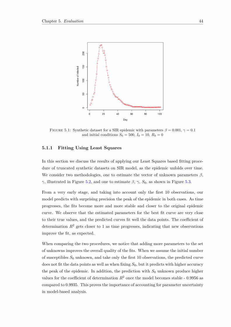
Chapter 5. Evaluation 44
Figure 5.1: Synthetic dataset for a SIR epidemic with parameters β = 0.001, γ = 0.1and initial conditions S0 = 500, I0 = 10, R0 = 0
5.1.1 Fitting Using Least Squares
In this section we discuss the results of applying our Least Squares based fitting proce-dure of truncated synthetic datasets on SIR model, as the epidemic unfolds over time.We consider two methodologies, one to estimate the vector of unknown parameters β,γ, illustrated in Figure 5.2, and one to estimate β, γ, S0, as shown in Figure 5.3.
From a very early stage, and taking into account only the first 10 observations, ourmodel predicts with surprising precision the peak of the epidemic in both cases. As timeprogresses, the fits become more and more stable and closer to the original epidemiccurve. We observe that the estimated parameters for the best fit curve are very closeto their true values, and the predicted curves fit well the data points. The coefficient ofdetermination R2 gets closer to 1 as time progresses, indicating that new observationsimprove the fit, as expected.
When comparing the two procedures, we notice that adding more parameters to the setof unknowns improves the overall quality of the fits. When we assume the initial numberof susceptibles S0 unknown, and take only the first 10 observations, the predicted curvedoes not fit the data points as well as when fixing S0, but it predicts with higher accuracythe peak of the epidemic. In addition, the prediction with S0 unknown produce highervalues for the coefficient of determination R2 once the model becomes stable - 0.9956 ascompared to 0.9935. This proves the importance of accounting for parameter uncertaintyin model-based analysis.

Chapter 5. Evaluation 45
Figure 5.2: Over-time Least Squares fitting of synthetic data on SIR model withunknown parameters β and γ.
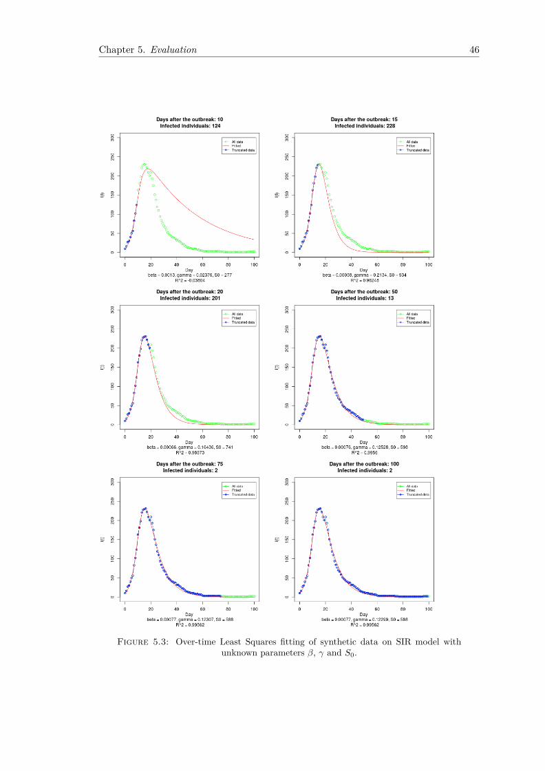
Chapter 5. Evaluation 46
Figure 5.3: Over-time Least Squares fitting of synthetic data on SIR model withunknown parameters β, γ and S0.
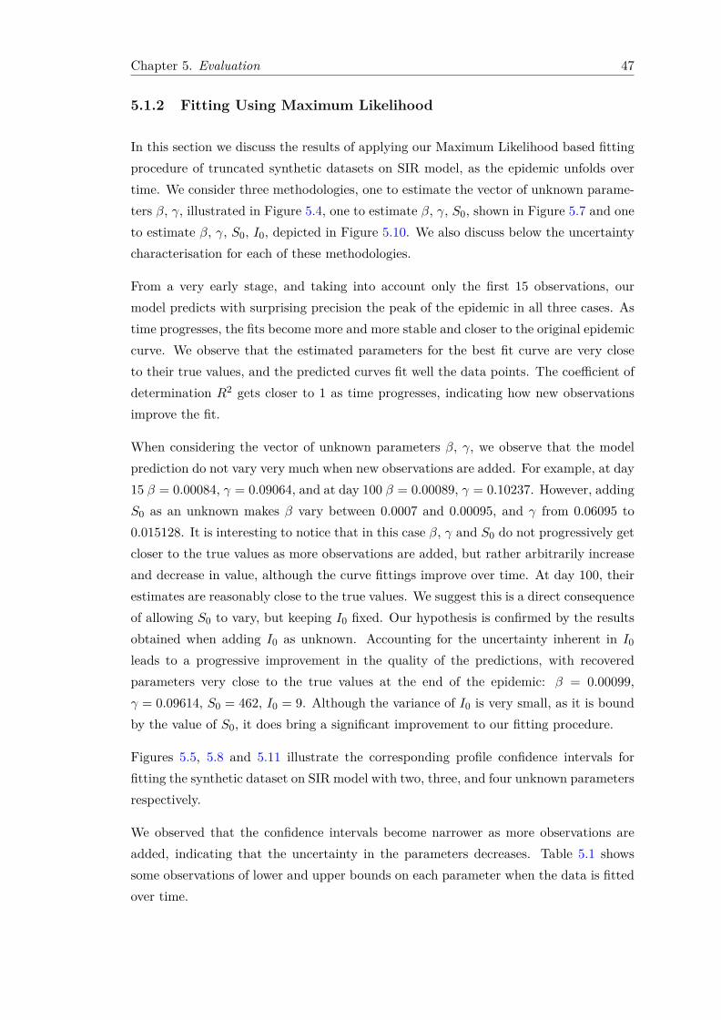
Chapter 5. Evaluation 47
5.1.2 Fitting Using Maximum Likelihood
In this section we discuss the results of applying our Maximum Likelihood based fittingprocedure of truncated synthetic datasets on SIR model, as the epidemic unfolds overtime. We consider three methodologies, one to estimate the vector of unknown parame-ters β, γ, illustrated in Figure 5.4, one to estimate β, γ, S0, shown in Figure 5.7 and oneto estimate β, γ, S0, I0, depicted in Figure 5.10. We also discuss below the uncertaintycharacterisation for each of these methodologies.
From a very early stage, and taking into account only the first 15 observations, ourmodel predicts with surprising precision the peak of the epidemic in all three cases. Astime progresses, the fits become more and more stable and closer to the original epidemiccurve. We observe that the estimated parameters for the best fit curve are very closeto their true values, and the predicted curves fit well the data points. The coefficient ofdetermination R2 gets closer to 1 as time progresses, indicating how new observationsimprove the fit.
When considering the vector of unknown parameters β, γ, we observe that the modelprediction do not vary very much when new observations are added. For example, at day15 β = 0.00084, γ = 0.09064, and at day 100 β = 0.00089, γ = 0.10237. However, addingS0 as an unknown makes β vary between 0.0007 and 0.00095, and γ from 0.06095 to0.015128. It is interesting to notice that in this case β, γ and S0 do not progressively getcloser to the true values as more observations are added, but rather arbitrarily increaseand decrease in value, although the curve fittings improve over time. At day 100, theirestimates are reasonably close to the true values. We suggest this is a direct consequenceof allowing S0 to vary, but keeping I0 fixed. Our hypothesis is confirmed by the resultsobtained when adding I0 as unknown. Accounting for the uncertainty inherent in I0
leads to a progressive improvement in the quality of the predictions, with recoveredparameters very close to the true values at the end of the epidemic: β = 0.00099,γ = 0.09614, S0 = 462, I0 = 9. Although the variance of I0 is very small, as it is boundby the value of S0, it does bring a significant improvement to our fitting procedure.
Figures 5.5, 5.8 and 5.11 illustrate the corresponding profile confidence intervals forfitting the synthetic dataset on SIR model with two, three, and four unknown parametersrespectively.
We observed that the confidence intervals become narrower as more observations areadded, indicating that the uncertainty in the parameters decreases. Table 5.1 showssome observations of lower and upper bounds on each parameter when the data is fittedover time.

Chapter 5. Evaluation 48
Data% β γ S0Lower Upper Lower Upper Lower Upper
25% 5.66e-04 8.47e-04 1.08e-01 1.93e-01 569 96250% 7.17e-04 8.36e-04 1.17e-01 1.35e-01 590 69275% 7.62e-04 8.68e-04 1.13e-01 1.26e-01 568 646100% 8.39e-04 9.47e-04 1.03e-01 1.14e-01 519 582
Table 5.1: Confidence Intervals for over-time fitting of synthetic data on SIR modelwith unknwon parameters β, γ, S0.
Figures 5.6 and 5.9 provide a graphical characterisation of the uncertainty when fittingthe synthetic dataset on SIR model with two and three unknown parameters respectively.The first one is a two-dimensional contour plot; the contour lines connect values that liewithin the same confidence interval. The second one is a three-dimensional isosurfaceplot; each surface embodies parameter values that lie in the same confidence intervalwithin a volume of space. Both these diagrams highlight the fact that the estimatedrange of possible values is wider as the confidence level increase.
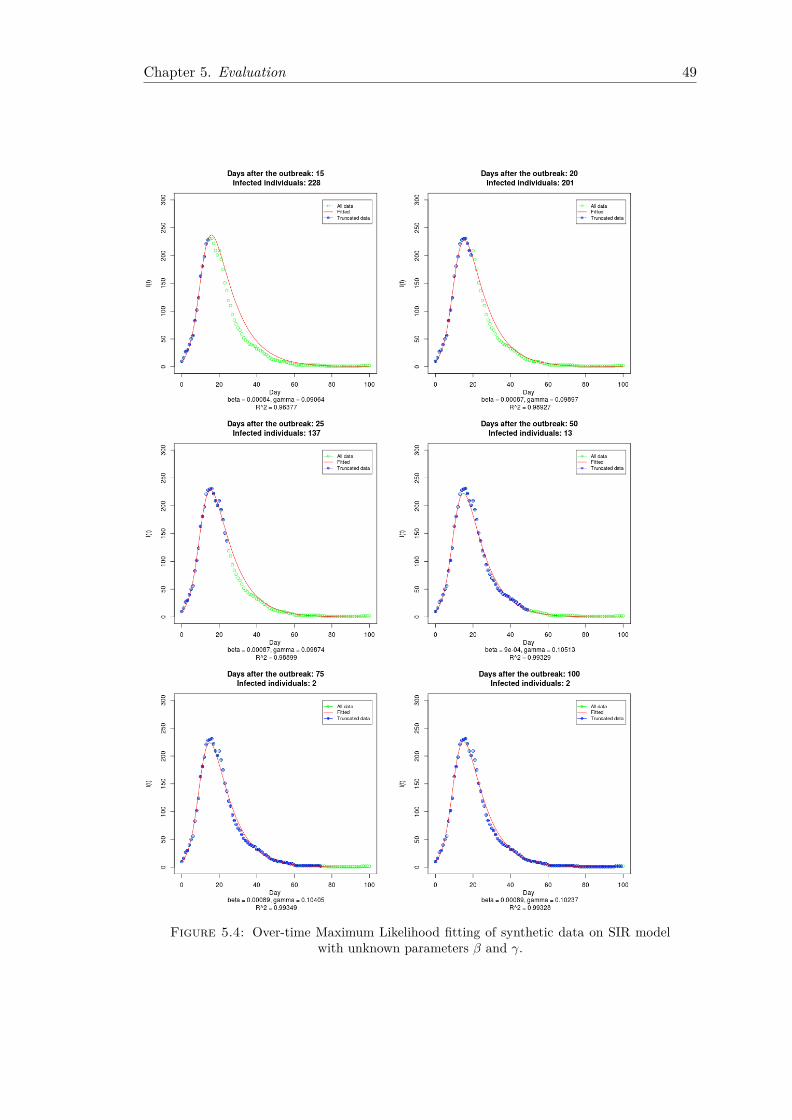
Chapter 5. Evaluation 49
Figure 5.4: Over-time Maximum Likelihood fitting of synthetic data on SIR modelwith unknown parameters β and γ.
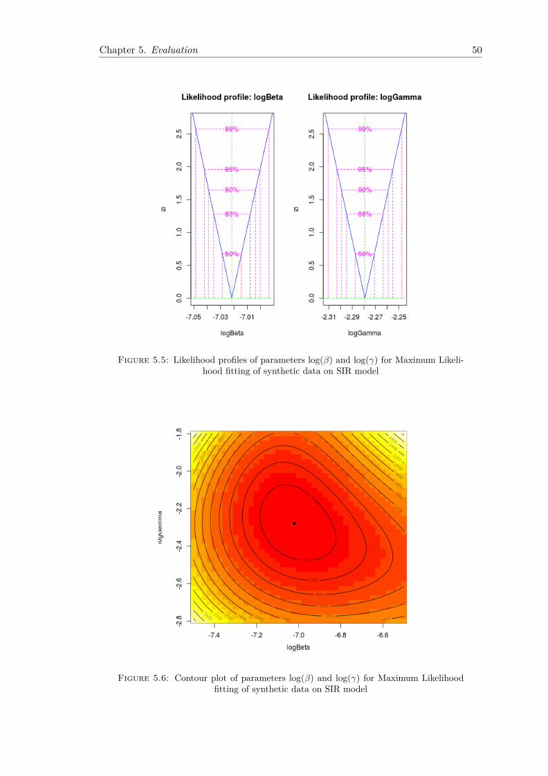
Chapter 5. Evaluation 50
Figure 5.5: Likelihood profiles of parameters log(β) and log(γ) for Maximum Likeli-hood fitting of synthetic data on SIR model
Figure 5.6: Contour plot of parameters log(β) and log(γ) for Maximum Likelihoodfitting of synthetic data on SIR model
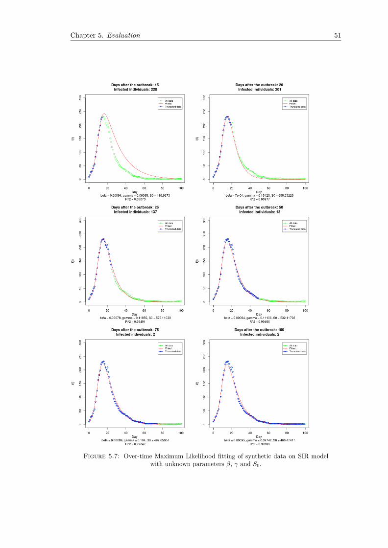
Chapter 5. Evaluation 51
Figure 5.7: Over-time Maximum Likelihood fitting of synthetic data on SIR modelwith unknown parameters β, γ and S0.
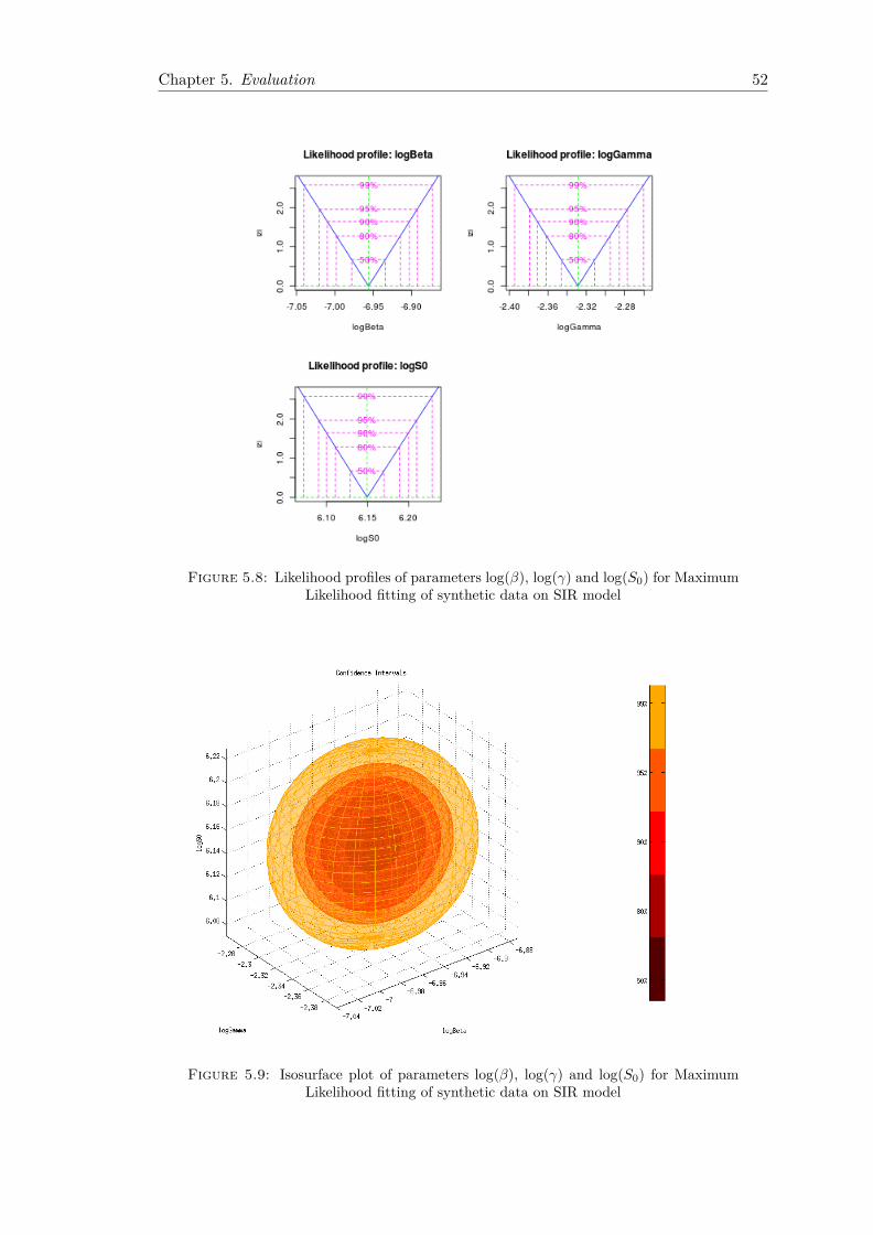
Chapter 5. Evaluation 52
Figure 5.8: Likelihood profiles of parameters log(β), log(γ) and log(S0) for MaximumLikelihood fitting of synthetic data on SIR model
Figure 5.9: Isosurface plot of parameters log(β), log(γ) and log(S0) for MaximumLikelihood fitting of synthetic data on SIR model
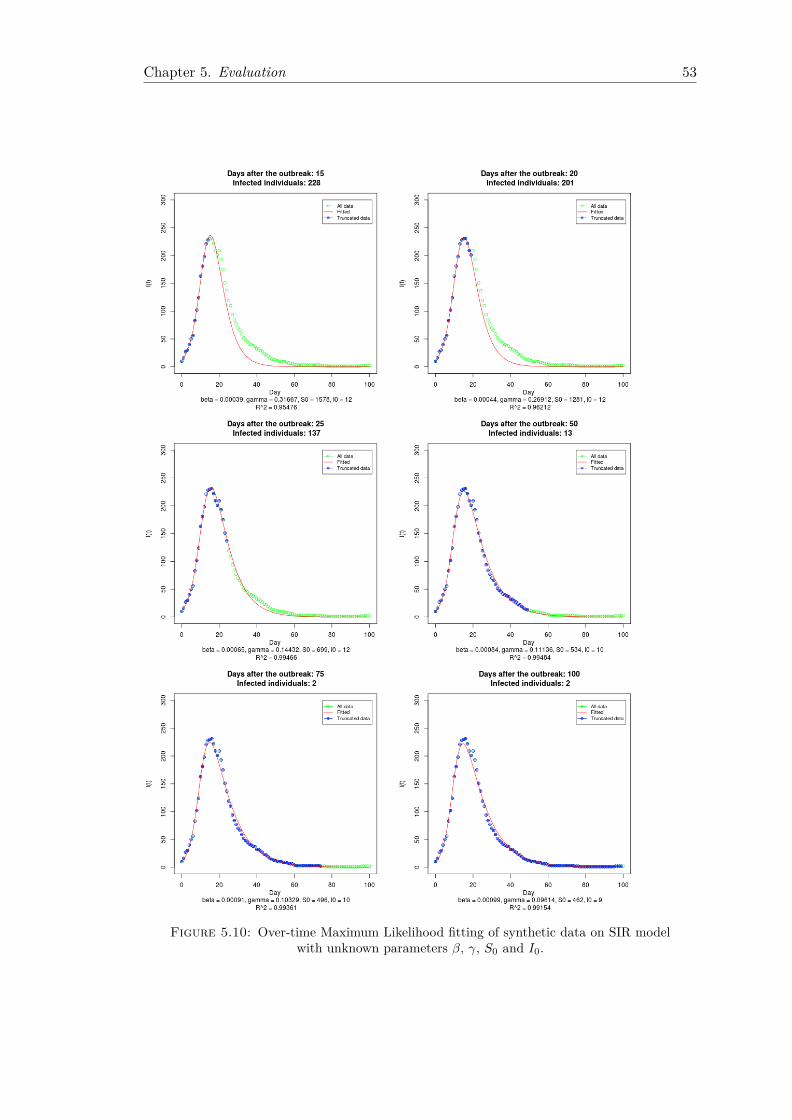
Chapter 5. Evaluation 53
Figure 5.10: Over-time Maximum Likelihood fitting of synthetic data on SIR modelwith unknown parameters β, γ, S0 and I0.
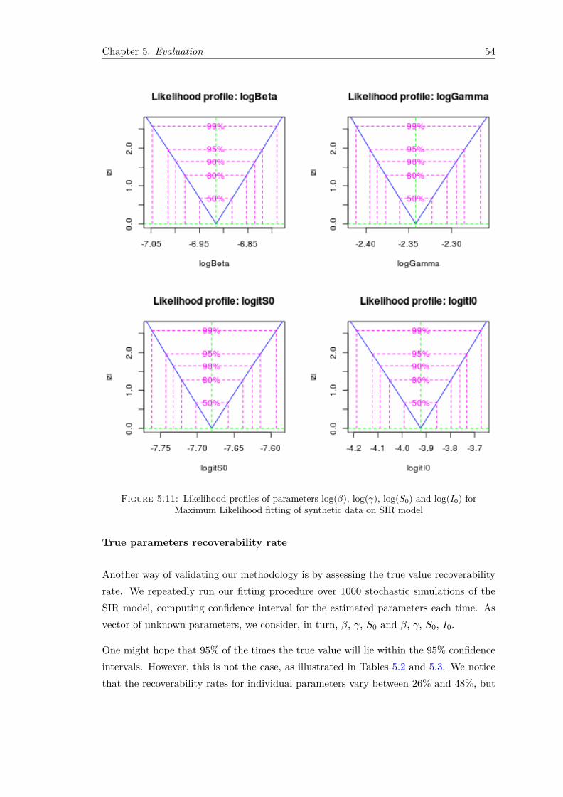
Chapter 5. Evaluation 54
Figure 5.11: Likelihood profiles of parameters log(β), log(γ), log(S0) and log(I0) forMaximum Likelihood fitting of synthetic data on SIR model
True parameters recoverability rate
Another way of validating our methodology is by assessing the true value recoverabilityrate. We repeatedly run our fitting procedure over 1000 stochastic simulations of theSIR model, computing confidence interval for the estimated parameters each time. Asvector of unknown parameters, we consider, in turn, β, γ, S0 and β, γ, S0, I0.
One might hope that 95% of the times the true value will lie within the 95% confidenceintervals. However, this is not the case, as illustrated in Tables 5.2 and 5.3. We noticethat the recoverability rates for individual parameters vary between 26% and 48%, but
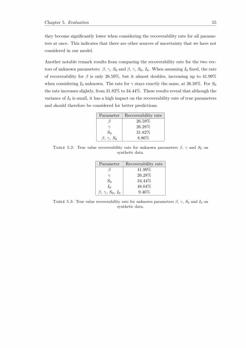
Chapter 5. Evaluation 55
they become significantly lower when considering the recoverability rate for all parame-ters at once. This indicates that there are other sources of uncertainty that we have notconsidered in our model.
Another notable remark results from comparing the recoverability rate for the two vec-tors of unknown parameters: β, γ, S0 and β, γ, S0, I0. When assuming I0 fixed, the rateof recoverability for β is only 26.59%, but it almost doubles, increasing up to 41.99%when considering I0 unknown. The rate for γ stays exactly the same, at 26.28%. For S0
the rate increases slightly, from 31.82% to 34.44%. These results reveal that although thevariance of I0 is small, it has a high impact on the recoverability rate of true parametersand should therefore be considered for better predictions.
Parameter Recoverability rateβ 26.59%γ 26.28%S0 31.82%
β, γ, S0 8.86%
Table 5.2: True value recoverability rate for unknown parameters β, γ and S0 onsynthetic data.
Parameter Recoverability rateβ 41.99%γ 26.28%S0 34.44%I0 48.04%
β, γ, S0, I0 9.46%
Table 5.3: True value recoverability rate for unknown parameters β, γ, S0 and I0 onsynthetic data.
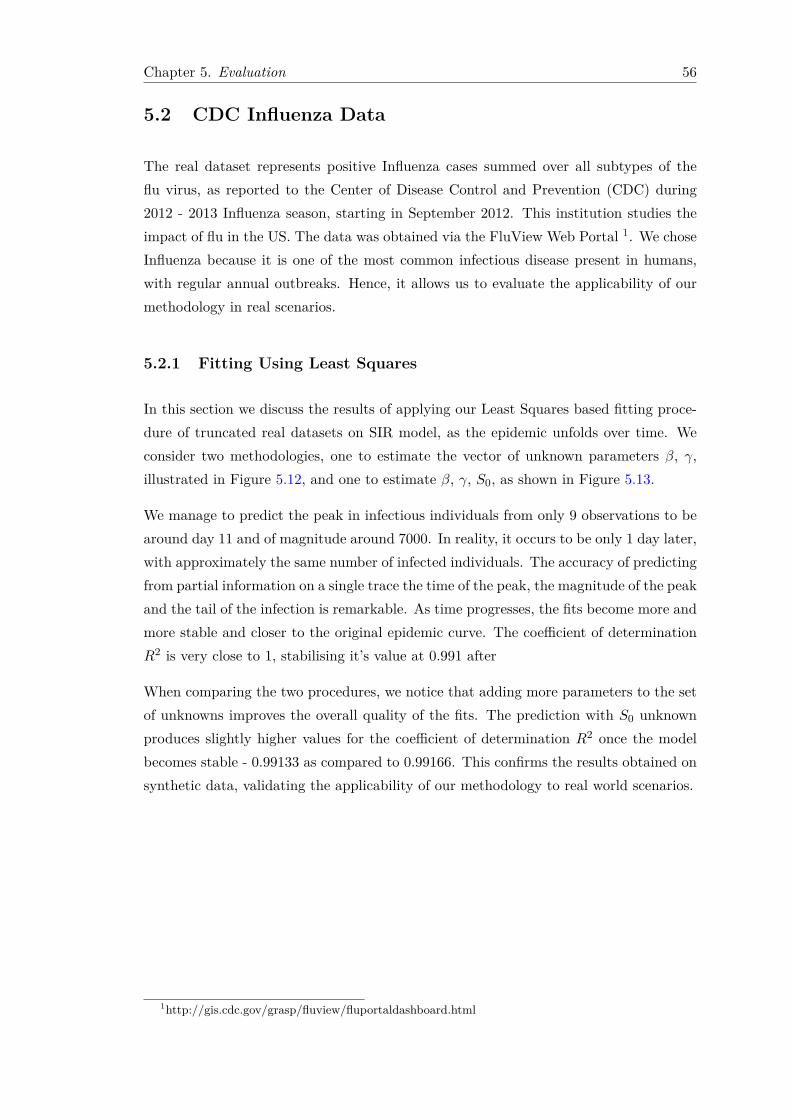
Chapter 5. Evaluation 56
5.2 CDC Influenza Data
The real dataset represents positive Influenza cases summed over all subtypes of theflu virus, as reported to the Center of Disease Control and Prevention (CDC) during2012 - 2013 Influenza season, starting in September 2012. This institution studies theimpact of flu in the US. The data was obtained via the FluView Web Portal 1. We choseInfluenza because it is one of the most common infectious disease present in humans,with regular annual outbreaks. Hence, it allows us to evaluate the applicability of ourmethodology in real scenarios.
5.2.1 Fitting Using Least Squares
In this section we discuss the results of applying our Least Squares based fitting proce-dure of truncated real datasets on SIR model, as the epidemic unfolds over time. Weconsider two methodologies, one to estimate the vector of unknown parameters β, γ,illustrated in Figure 5.12, and one to estimate β, γ, S0, as shown in Figure 5.13.
We manage to predict the peak in infectious individuals from only 9 observations to bearound day 11 and of magnitude around 7000. In reality, it occurs to be only 1 day later,with approximately the same number of infected individuals. The accuracy of predictingfrom partial information on a single trace the time of the peak, the magnitude of the peakand the tail of the infection is remarkable. As time progresses, the fits become more andmore stable and closer to the original epidemic curve. The coefficient of determinationR2 is very close to 1, stabilising it’s value at 0.991 after
When comparing the two procedures, we notice that adding more parameters to the setof unknowns improves the overall quality of the fits. The prediction with S0 unknownproduces slightly higher values for the coefficient of determination R2 once the modelbecomes stable - 0.99133 as compared to 0.99166. This confirms the results obtained onsynthetic data, validating the applicability of our methodology to real world scenarios.
1http://gis.cdc.gov/grasp/fluview/fluportaldashboard.html
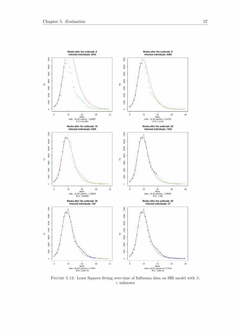
Chapter 5. Evaluation 57
Figure 5.12: Least Squares fitting over-time of Influenza data on SIR model with β,γ unknown
Chapter 5. Evaluation 58
Figure 5.13: Least Squares fitting over-time of Influenza data on SIR model with β,γ, S0 unknown
Chapter 5. Evaluation 59
5.2.2 Fitting Using Maximum Likelihood
In this section we discuss the results of applying our Maximum Likelihood based fittingprocedure of truncated real datasets on SIR model, as the epidemic unfolds over time.We consider two methodologies, one to estimate the vector of unknown parameters β,γ, S0, shown in Figure 5.14, and one to estimate β, γ, S0, I0, illustrated in Figure 5.17.We also discuss below the uncertainty characterisation for each of these methodologies.
The experiments on real data confirmed the results obtained on synthetic datasets. Themodel proved highly accurate in predicting from partial information on a single trace.Considering only 20% of the observations, it accurately predicts the time of the peak,its magnitude, and the tail of the infection. As before, the confidence intervals for theparameter estimates become narrower as more observations are added, indicating thatthe uncertainty in the parameters decreases. Likelihood profiles, and corresponding iso-surface plot are illustrated in Figures 5.15, 5.16, 5.18. Table 5.4 shows some observationsof lower and upper bounds on each parameter when the data is fitted over time.
Table 5.4: Confidence Intervals for over-time Influenza data (* - non convergence)
Data% β γ S0Lower Upper Lower Upper Lower Upper
25% * * * * * *50% 2.95e-05 3.22e-05 3.46e-01 3.81e-01 26769 3011875% 3.50e-05 3.69e-05 2.90e-01 3.06e-01 22091 23515100% 3.53e-05 3.70e-05 2.90e-01 3.03e-01 22031 23292
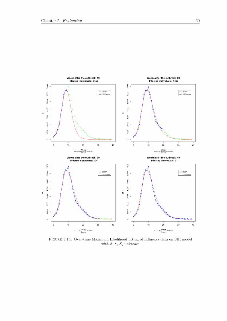
Chapter 5. Evaluation 60
Figure 5.14: Over-time Maximum Likelihood fitting of Influenza data on SIR modelwith β, γ, S0 unknown
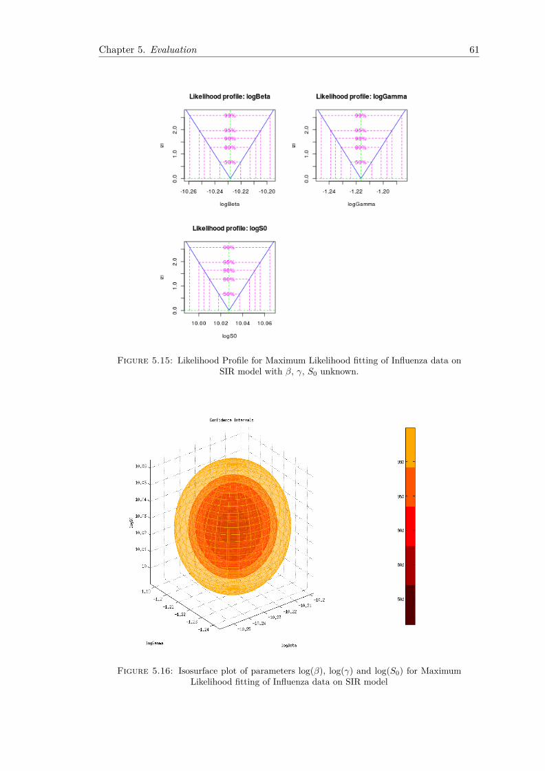
Chapter 5. Evaluation 61
Figure 5.15: Likelihood Profile for Maximum Likelihood fitting of Influenza data onSIR model with β, γ, S0 unknown.
Figure 5.16: Isosurface plot of parameters log(β), log(γ) and log(S0) for MaximumLikelihood fitting of Influenza data on SIR model
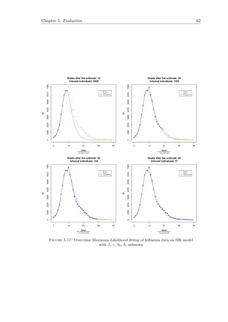
Chapter 5. Evaluation 62
Figure 5.17: Over-time Maximum Likelihood fitting of Influenza data on SIR modelwith β, γ, S0, I0 unknown
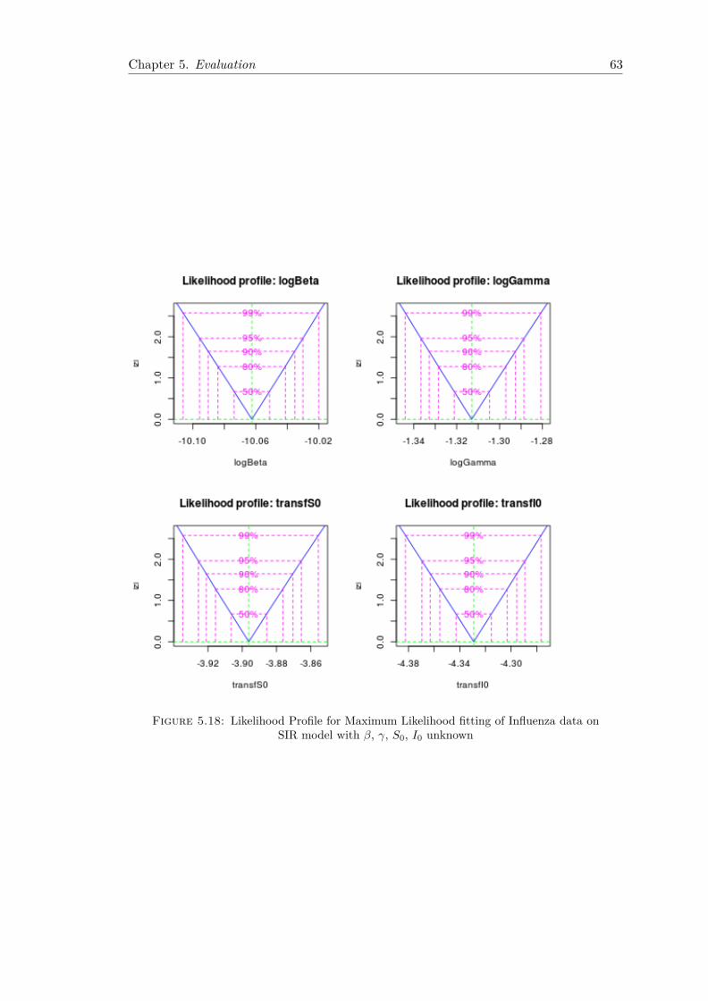
Chapter 5. Evaluation 63
Figure 5.18: Likelihood Profile for Maximum Likelihood fitting of Influenza data onSIR model with β, γ, S0, I0 unknown
Chapter 6
Conclusion
6.1 Contributions
Researching applications of mathematical modelling techniques to epidemic phenomenaproved to be a challenging, but rewarding task. While working on this project, we hadthe opportunity to deal with difficult aspects of statistical estimation of parameters andcharacterising their uncertainty. We tackled the challenge of estimating key parameters,such as the initial number of susceptible and infected individuals in the SIR model.Traditionally, they are assumed to be known or can be inferred from the context, butthis approach is not feasible for modern outbreaks. Moreover, we had the pleasure toaddress unanswered questions of wide interest in areas such as contingency planningregarding the importance of uncertainty characterisation.
We initially implemented a Least Square based methodology for on-the-fly epidemicfitting on SIR models from a single trace. The method was validated using both syntheticand real data. From very early stages, our model predicted with surprising precision thepeak of the epidemic. The estimated parameters for the best fit curve were very closeto their true values, and the predicted curves fitted well the data points.
The main contribution of this project is a generic Maximum Likelihood based approachthat characterises rigorously the uncertainty inherent in parameter estimates. It is ad-dressed to on-the-fly epidemic fitting of SIR models from a single trace, and yieldsconfidence intervals on parameter values. Opposite to traditional epidemiological mod-elling techniques, our approach is fully automated. We also provide estimates for keyparameters such as the number of initial susceptibles and the initial number of infectedin the population. Visualising the fitted parameters gives rise an isosurface plot of thefeasible parameter ranges corresponding to each confidence level.
64

Chapter 5. Conclusion 65
6.2 Future Work
We believe there are many areas of improvement for our project. In this section, weoutline some ideas for potential extensions and further research:
• Estimate the starting time of the epidemic A potential extension to our method-ology is to incorporate uncertainty inherent in the starting time of the epidemic.Currently, we assume this t0 to be fixed, but in reality we do not know its truevalue. Traditionally, laborious manual work is being undertaken to detect the in-dex case associated with an infectious disease spread in order to determine whendid the epidemic emerge. Besides being very time consuming, such methods arealso individuals being able to recall and provide complete, accurate informationregarding their personal relationships.
• Implement uncertainty characterisation methodologies for other compartmentalmodels So far, we have only focused on the SIR model, which is the most simpleof the compartmental models. Another potential extension would be to developanalog methodologies for other, more complex compartmental models. The abil-ity to characterise uncertainty in more realistic models would add great value tomodel-based analysis for policy and decision making.
• Develop a simulation-based methodology It is expected that real systems are likelyto exhibit different characteristics than the ideal ones assumed by the classical SIRmodel; for example, real systems may feature time-varying parameters and thehomogeneous mixing assumption may not apply. Nevertheless, the models mayhave utility in predicting the stochastic impact of candidate interventions in realsystems with bounds [30], and a simulation-based methodology for this will couldbe a starting point for future work.
• Investigate model selection methodologies Development of complex epidemiologicalmodels increased the popularity of large scale simulations of epidemic spread in theliterature. Accurate predicting on how an infection may spread is limited by thelack of rigorous approaches to validate such models and assess which one would bebest for a particular problem. Furthermore, if we encounter a high goodness-of-fitfor a set of observed data, how can we infer which specific model has produced it?Such questions do not have an answer yet and could be addressed in future work.
Bibliography
[1] A.J. Tatem, D.J. Rogers, and S.I. Hay. Global transport networks and infectiousdisease spread. In Global Mapping of Infectious Diseases: Methods, Examplesand Emerging Applications, volume 62 of Advances in Parasitology, pages 293 –343. Academic Press, 2006. Available online at http://www.sciencedirect.com/
science/article/pii/S0065308X0562009X.
[2] S. Scott and C. Duncan. Return of the Black Death. The World’s Greatest SerialKiller. Wiley, 2004.
[3] T.D. Hollingsworth, N.M. Ferguson, and R.M. Anderson. Frequent travelers andrate of spread of epidemics. Emerging Infectious Diseases, 19(9). Available onlineat http://wwwnc.cdc.gov/eid/article/13/9/07-0081.htm.
[4] M. Gladwell. The Tipping Point: How Little Things Can Make a Big Difference.Little Brown, 2000.
[5] J. Cannarella and J.A. Spechler. Epidemiological modeling of online social networkdynamics. Available online at http://arxiv.org/abs/1401.4208, January 2014.
[6] Facebook statistics, 2014. Available online at http://www.statisticbrain.com/
facebook-statistics/. Accessed on January 30, 2014.
[7] R.M. Christley, M. Mort, B. Wynne, J.M. Wastling, A.L. Heathwaite, R. Pickup,Z. Austin, and Latham S.M. “wrong, but useful”: Negotiating uncertainty ininfectious disease modelling. PLoS NE, 8(10), 10 2013. Available online athttp://dx.doi.org/10.1371%2Fjournal.pone.0076277.
[8] M. Nika, G. Ivanova, and W.J. Knottenbelt. On celebrity, epidemiology and theinternet. In Proc. 7th International Conference on Performance Evaluation Method-ologies and Tools (VALUETOOLS), Turin, Italy, December 2013.
[9] Matt J Keeling and Ken TD Eames. Networks and epidemic models. Journal ofthe Royal Society Interface, 2(4):295–307, 2005.
66
Bibliography 67
[10] M.J. Keeling and P. Rohani. Modeling Infectious Diseases in Humans and Animals.Princeton University Press, 2008.
[11] M.J. Keeling. Models of foot-and-mouth disease. Proceedings of the Royal Society,Biological Sciences, 272(1569). Available online at http://www.ncbi.nlm.nih.
gov/pmc/articles/PMC1564112/?report=classic.
[12] Emilia Vynnycky and Richard White. An introduction to infectious disease mod-elling. Oxford University Press, 2010.
[13] W. O. Kermack and A. G. McKendrick. A contribution to the mathematical the-ory of epidemics. Proceedings of the Royal Society of London. Series A, 115(772):700–721, 1927. Available online at http://rspa.royalsocietypublishing.org/
content/115/772/700.short.
[14] H.W. Hethcote. The mathematics of infectious diseases. SIAM Rev., 42(4):599–653, December 2000. Available online at http://dx.doi.org/10.1137/
S0036144500371907.
[15] J. M. Heffernan, R. J. Smith, and L. M. Wahl. Perspectives on the basic re-productive ratio. Journal of the Royal Society, Interface / the Royal Society, 2(4):281–293, September 2005. Available online at http://dx.doi.org/10.1098/rsif.
2005.0042.
[16] J. Lloyd-Smith. Parameter estimation, uncertainty, model fitting, model selec-tion, and sensitivity and uncertainty analysis, June 2007. Lecture notes for theDIMACS/SACEMA/AIMS Advanced Study Institute, available online at dimacs.
rutgers.edu/Workshops/AIMS/slides/JLS_ASI_6.pdf.
[17] Daniel T Gillespie. Exact stochastic simulation of coupled chemical reactions. Thejournal of physical chemistry, 81(25):2340–2361, 1977.
[18] A.F. Burns and W.C. Mitchell. Measuring Business Cycles. National Bureau ofEconomic Research, Inc, 1946. Available online at http://EconPapers.repec.
org/RePEc:nbr:nberbk:burn46-1.
[19] M. Aoki. New Approaches to Macroeconomic Modeling: Evolutionary StochasticDynamics, Multiple Equilibria, and Externalities as Field Effects. Cambridge Uni-versity Press, June 1996.
[20] F. Tramontana and M. Gallegati. Economics as a compartmental system: a simplemacroeconomic example. Working Papers 1011, University of Urbino Carlo Bo,Department of Economics, 2010. Available online at http://EconPapers.repec.
org/RePEc:urb:wpaper:10_11.
Bibliography 68
[21] Bob Duffy, Kevin Regan, Steve Coulombe, and John Yozzo. A realcliffhanger. 2012 retail report. Technical report, FTI Consulting, 2012. Avail-able online at http://origin.fticonsulting.co/global2/media/collateral/
united-states/2012-annual-retail-report-a-real-cliffhanger.pdf.
[22] C.C. Zou, W. Gong, and D. Towsley. Code red worm propagation modelingand analysis. In Proceedings of the 9th ACM Conference on Computer andCommunications Security, CCS 2002, pages 138–147. Available online at http:
//doi.acm.org/10.1145/586110.586130.
[23] L.X. Yang and X. Yang. A new epidemic model of computer viruses. Com-munications in Nonlinear Science and Numerical Simulation, 19(6):1935 – 1944,2014. Available online at http://www.sciencedirect.com/science/article/
pii/S1007570413004656.
[24] J.C. Lagarias, J.A. Reeds, M.H. Wright, and P.E. Wright. Convergence properties ofthe nelder-mead simplex method in low dimensions. SIAM Journal of Optimization,9:112–147, 1998. Available online at http://citeseerx.ist.psu.edu/viewdoc/
summary?doi=10.1.1.120.6062.
[25] W.D. Flanders and D.G. Kleinbaum. Basic models for disease occurrence in epi-demiology. International Journal of Epidemiology, 24(1):1–7, 1995. Available onlineat http://ije.oxfordjournals.org/content/24/1/1.abstract.
[26] B. Bolker and S. Ellner. Likelihood and all that, for disease ecologists. Tutorialdistributed by The King Laboratory of Theoretical Ecology & Evolution at theUniversity of Michigan, June 2011. Available online at http://kinglab.eeb.lsa.
umich.edu/EEID/eeid/ecology/mle_2012.pdf.
[27] R. Dolgoarshinnykh. Introduction to epidemic modelling. Lecture Notes for a Grad-uate Course in Epidemic Modelling. Department of Statistics, Columbia University,2005.
[28] T. Seidenfeld. Philosophical problems of statistical inference: Learning from RAFisher. Number 22. Springer, 1979.
[29] D. Patterson. Profile likelihood confidence intervals for glm’s. Lecture Notesfor Mathematical Statistics Course, Department of Mathematical Sciences, Uni-versity of Montana, 2011. Available online at www.math.umt.edu/patterson/
ProfileLikelihoodCI.pdf.
[30] T. L. Burr and G. Chowell. Observation and model error effects on parameter es-timates in susceptible-infected-recovered epidemiological models. Far East Journalof Theoretical Statistics, 19(2):163–183, 2013.

Bibliography 69
[31] F. Brauer. Compartmental models in epidemiology. In Mathematical Epidemi-ology, volume 1945 of Lecture Notes in Mathematics, pages 19–79. SpringerBerlin Heidelberg, 2008. Available online at http://dx.doi.org/10.1007/
978-3-540-78911-6_2.
[32] L. M. A. Bettencourt, A. Cintron-Arias, D. I. Kaiser, and C. Castillo-Chavez. ThePower of a Good Idea: Quantitative Modeling of the Spread of Ideas from Epidemi-ological Models. 2005. doi: 10.2172/990668.