On the Feasibility of FPGA Acceleration ofMolecular Dynamics Simulations

Technical Report (v0.1)

Michael Schaffner†, Luca Benini††ETH Zurich, Integrated Systems Lab IIS, Zurich, Switzerland

Abstract—Classical molecular dynamics (MD) simulations areimportant tools in life and material sciences since they allowstudying chemical and biological processes in detail. However,the inherent scalability problem of particle-particle interactionsand the sequential dependency of subsequent time steps renderMD computationally intensive and difficult to scale. To thisend, specialized FPGA-based accelerators have been repeatedlyproposed to ameliorate this problem. However, to date none of theleading MD simulation packages fully support FPGA accelerationand a direct comparison of GPU versus FPGA accelerated codeshas remained elusive so far.

With this report, we aim at clarifying this issue by comparingmeasured application performance on GPU-dense compute nodeswith performance and cost estimates of a FPGA-based single-node system. Our results show that an FPGA-based system canindeed outperform a similarly configured GPU-based system, butthe overall application-level speedup remains in the order of 2×due to software overheads on the host. Considering the price forGPU and FPGA solutions, we observe that GPU-based solutionsprovide the better cost/performance tradeoff, and hence pureFPGA-based solutions are likely not going to be commerciallyviable. However, we also note that scaled multi-node systemscould potentially benefit from a hybrid composition, where GPUsare used for compute intensive parts and FPGAs for latency andcommunication sensitive tasks.

I. INTRODUCTION

Classical molecular dynamics (MD) simulations [1] are im-portant tools in life and material sciences since they allowstudying chemical and biological processes in detail. Forexample, this enables researchers to study drug-target bindingsfor drug discovery purposes [2] or to analyze protein foldingprocesses to understand their biological function [3].

However, MD is computationally intensive and difficult toscale due to the sequential dependency between subsequenttimesteps and the many particle-particle interactions. Thetimescales of interest are often orders of magnitude larger thanthe simulation time steps (i.e., ns or µs timescales versus fstime steps), which results in long simulation times even onHPC computing infrastructure.

To this end, several approaches have been pursued toimprove simulation performance, ranging from novel algo-rithms to approximate forces between particles [4] over al-gorithmic tweaks [5] and biasing methods such as enhancedsampling methods [6], to custom hardware solutions, such asthe MDGRAPE systems from Riken [7] and the Anton-1/2supercomputers developed by D.E. Shaw Research LLC [3],[8], [9]. However, we observe that algorithmic improvementsare often very problem specific, and it often takes a long timeuntil they are adopted by major production software packages.

Hence, the core algorithms used in classical MD simulationshave largely remained in recent years, and most simulationspeed improvements are due to the use of MPI parallelizationin combination with GPGPUs that handle the computationallydominant parts. Specialized supercomputers such as the Antonsystems are very inaccessible and expensive, and are hence notwidely used today.

Besides these MPI and GPU-based solutions, FPGA accel-erators have repeatedly been proposed as a viable alternativeto accelerate the compute intensive parts [10–22] . However,these studies only show estimated or measured speedup withrespect to older CPU implementations. To date none of theleading MD simulation packages fully support FPGA accel-eration [23] and a direct comparison of GPU versus FPGAaccelerated codes has remained elusive so far.

This report aims at shedding some light onto the questionswhether and how FPGAs could be used to accelerate classicalMD simulations in the scope of biochemistry, and whethersuch a solution would be commercially viable. To this end,we revisit existing FPGA architectures, model their behavioron current FPGA technology and estimate the performanceand price of an FPGA accelerated system in order to comparewith GPU accelerated solutions. We focus on single nodesystems in this report (possibly carrying several acceleratorcards) since these represent the most common configurationemployed today1. Typical MD problems with in the order of100k atoms do not scale well across several nodes, and henceit is most economic to run these simulations on accelerator-dense single node systems.

Our results show that, in principle, FPGAs can be used toaccelerate MD, and we estimate full application-level speedupsin the order of 2× with respect to GPU-based solutions.However, our estimates also indicate that this speedup islikely not high enough to compensate for the increased costand reduced flexibility of FPGA-based solutions. Hence weconclude that FPGAs are likely not well suited as a replace-ment for GPU accelerators. However, we observe that otheraspects of FPGAs like the low-latency networking capabilitiescould be leveraged to augment scaled multi-node systems andameliorate scalability issues by providing network-computecapabilities in addition to GPU acceleration.

This report is structured in three main sections: Sec. IIsummarizes background and related work, performance bench-marks of two widely used software packages are given inSec. III, and in Sec. IV we provide the FPGA estimates andcomparisons with GPU-based systems.

arX

iv:1

808.

0420

1v1

[cs

.DC

] 8

Aug

201

8

II. BACKGROUND AND RELATED WORK

A. Classical MD

This section gives a brief overview of MD, for more detailswe refer to [1], [2], [24], [25].

1) Simulation Loop and Force-Fields

A typical biomolecular MD simulation consists of a macro-molecule that is immersed in a solvent (e.g., water). Each atomin the system is assigned a coordinate xi, velocity vi andacceleration ai. The aim of MD is to simulate the individualtrajectories of the atoms, and this is done by integrating theforces acting on each particle. The integration is carried out indiscrete timesteps, with a resolution in the order of 2 fs, andthe forces are calculated by taking the negative derivative ofa potential function V w.r.t. to each particle coordinate xi:

fi (t) = miai (t) = −∂V (x (t))

∂(xi (t)(1)

where the potential function is based on classical Newtonianmechanics. The potential typically comprises the followingterms:

V =

bonds∑i

kl,i2

(li − l0,i)2 +angles∑i

kα,i2

(αi − α0,i)2

+

torsions∑i

(M∑k

Vik2

cos (nik · θik − θ0,ik)

)

+

pairs∑i,j

εij

((r0,ijrij

)12

− 2

(r0,ijrij

)6)

+

pairs∑i,j

qiqj4πε0εrrij

(2)

Such a set of functions and the corresponding parameteriza-tion is often also called a force-field (examples for specificforce field instances are CHARMM36m, GROMOS36 or AM-BERff99). The first three terms in (2) cover the interactionsdue to bonding relationships and are hence also called thebonded terms. The last two terms cover the van der Waalsand electrostatic (Coulomb) interactions, and are hence calledthe non-bonded terms. We can already anticipate from theseequations that the non-bonded terms will play a dominantrole during force calculation since it is a particle-particle (PP)problem with O(N2). The bonded terms are usually muchless intensive (O(N)) since we do not have bonds among allparticles in the system.

Most simulations are carried out using periodic boundaryconditions (PBC) in order to correctly simulate the bulkproperties of the solvent. This means that the simulation cellcontaining the N -particle system above is repeated infinitelymany times in all directions, which has implications on thealgorithms used for the non-bonded forces.

A typical MD simulation has an outer loop that advances thesimulation time in discretized steps in the order of fs, and ineach time step, all forces in the system have to be calculated,

1http://ambermd.org/gpus/recommended hardware.htm

the equations of motion have to be integrated, and additionalconstraints2 have to be applied before restarting the loop.

2) Evaluation of Non-bonded Interactions

The first term with 1/r12 and 1/r6 modelling the Van derWaals interaction decays very quickly. Therefore, a cutoffradius r can be used (usually in the order of 8-16 Angstroms),and only neighboring particles within the spanned sphere areconsidered during the evaluation of this term.

The Coulomb interaction on the other hand is more difficultto handle, as it decays relatively slowly (1/r). Earlier methodsalso just used a cutoff radius, but this may introduce significanterrors. To this end, different algorithms that leverage the peri-odic arrangement have been introduced. The most prominentone is the Ewald sum method (and variations thereof). This isbasically a mathematical trick to split the Coulomb interactioninto two separate terms: a localized term that is evaluatedin space-domain, and a non-local term that is evaluated inthe inverse space (i.e., in the spatial frequency domain / k-space). This decomposition enables efficient approximationmethods that have computational complexity O(N log(N))instead of O(N2). One such method that is widely usedtogether with PBC today is called Particle-Mesh Ewald (PME)[29–32]. Basically, the spatial term is handled locally with acutoff radius (same as for the Van der Waals term above),and the second is approximated using a gridded interpolationmethod combined with 3D FFTs (hence the O(N log(N)))complexity). The spatial term is sometimes also called theshort-range interaction part, whereas the inverse space term iscalled the long-range interaction part.

In terms of computation and communication, the non-bonded terms are the heavy ones, and consist of two cutoff-radius limited PP problems, and two 3D FFT problems. Aswe shall see later in Sec. III, these non-bonded forces accountfor more than 90% of the compute time in an unparallelizedMD simulation. Moreover, an intrinsic problem of MD is thatthe simulation time steps are sequentially dependent, whichinherently limits the parallelizability, and means that we haveto parallelize a single time step as good as possible (whichessentially creates a communication problem). Note that thedataset sizes are very manageable and only in the order of acouple of MBytes.

3) Other Approaches

Today, the most serious contenders for replacing PME elec-trostatics seem to be fast multipole methods (FMM) [29],[33–36], multi-level summation methods (MSM) [4], [37] andmulti-grid (MG) methods [38]:• FMM: The FMM makes use of a hierarchical tree decom-

position of simulation space and interacts particles withmultipole approximations of the farfield, thereby givingrise to O (N) complexity. For low order expansions,the multipole approximation of the electrostatic potentialfunction has large discontinuities. This leads to drifts

2Constraints are usually used to eliminate high-frequency oscillations of Hatoms that would lead to integration issues otherwise, see also [26–28].

of the total energy over time, and this violation ofenergy conservation is not acceptable in MD applications.To resolve this issue, one has to resort to high orderexpansions that are more accurate, but also more complexto calculate. With sufficiently high expansion orders, theFMM can be slower [4], [30] than fast PME algorithms inthe important range of N = 10k - 100k particles (despitethe fact that FMM has better asymptotic complexity thanPME)3.

• MG: These methods discretize the Laplace operator andsolve the resulting linear system with a multigrid solver,which results in linear complexity as well. however, thesemethods suffer from relatively large discretization errorscompared with FFT methods, thereby leading to clearenergy drifts that need to be corrected for [33].

• MSM: This method splits the interaction kernelssmoothly into a sum of partial kernels of increasingrange and decreasing variability, and the long-range partsare interpolated from grids of increasing coarseness, andhence MSM provides O (N) complexity, too. The MSMis relatively new, and hence not widely adopted yet. Itis unclear how it compares to PME in speed, but it isshown to provide better performance than FMM in thecase of highly parallel computation and it can be usedfor nonperiodic systems, where FFT-based methods donot apply [4].

Due to the reasons mentioned, FMM, MSM and MG methodshave not yet been widely adopted by common softwarepackages. Another reason is that in a direct comparison[33], FFT-based methods are still among the most efficientin performance and stability – and hence it is difficult tomotivate a migration to an new experimental algorithm if it notabsolutely required. The log (N) contribution of FFT basedmethods does not seem to be visible for common system sizes.Hence, for single-node systems not operating at scale, FFT-based methods still seem to be the best algorithmic choice forsimulations with PBC due to their efficiency and algorithmicsimplicity. As we will see later in Sections III and IV, one wayto address the communication bottleneck within PME can beaddressed by dedicating it to a single FPGA or GPU, whereit can be executed at very high speeds.

4) Classical versus Ab-Initio MD

Note that classical MD should not to be confused with ab-initioMD (AIMD) that operates on quantum-mechanical potentialapproximations. While AIMD has the advantages of beingmore accurate and not requiring explicit parameterization, it isalso computationally much more involved and hence limitedto small MD systems comprising a few 100 to 1000 particles.Classical MD works on a coarser abstraction4 by employingclassical mechanics in the form of force-fields that can beevaluated more efficiently, hence allowing to simulate larger

3See also these LAMMPS and GROMACS forum entries: http://lammps.sandia.gov/threads/msg72001.html, http://www.gromacs.org/Developer Zone/Programming Guide/Fast multipole

4Mixed simulation modes where some potential calculations of classicalMD are augmented with QM are possible, but not considered in this report.

systems with up to several 100k atoms. Although classical MDsimluations are less accurate than their AIMD counterparts,they are often accurate enough for many biomolecular systems,where AIMD would not be feasible due to amount of particlesinvolved. The drawback of classical MD is that the force-fieldsneed to be parameterized with experimental data, and they canoften not model chemical reactions as the bonds are static.

An interesting new algorithmic development for AIMD-based approaches is to use neural networks (NN) to acceleratethe evaluation of the quantum-mechanical potentials [39].

B. Dedicated ASICs for classical MD

There exist only a few dedicated systems that have beenbuilt to enhance MD simulation performance. Two older onesare the MD-ENGINE [40] and MDGRAPE-3 [41]. The MD-ENGINEis a simple ASIC coprocessor that evaluates non-bonded forces only (with a non-optimized Ewald sum methodwhich is O

(N2)). Several such accelerators can be attached

to a SPARC host system that carries out the rest of thecalculations. Compared to newer architectures, the system doesnot scale well since it is still based on the a direct Ewaldsum method. the interpolation units use a combination offixed point and extended single-precision (40 bit) FP formats.MDGRAPE-3 is another MD co-processor chip which issimilar to the MD-ENGINE above in the sense that only thenon-bonded portion in the MD force calculation is accelerated,and they still use the direct Ewald sum method, which isaccurate, but O(N2). However, the complete system is muchlarger than previous ones: the complete system comprises256 compute nodes equipped with 2 Itanium class CPUs andtwo MDGRAPE boards with 24 chips each. This results in acluster with 512 CPUs and 6144 special purpose MDGRAPEchips. Also, they use a ring interconnect topology on eachMDGRAPE board, which facilitates reduction operations suchas force summation on one board.

Apart from these older instances above, there are also a fewmore recent incarnations of such special purpose machinesthat leverage complete SoC integration to accelerate MD ina more holistic fashion. The most notable machines are theAnton-1 [3], [42], [43] and Anton-2 [9] computers by D.E.Shaw Research LLC. The MDGRAPE-4 chip from Riken [7]is another special purpose SoC for MD that has similaritieswith the Anton chips, but the project does not seem to be assuccessful as Anton.

Both Anton generations are similar from a conceptualviewpoint, so we will mainly refer to numbers from Anton-2 inthe following. The system configuration comprises a set of 512compute nodes, interconnected with a 8×8×8 3D Torus, andeach compute node consists of one Anton-2 ASIC fabricated in40 nm. The 3D torus arrangement allows for natural problemmapping using a domain decomposition and facilitates com-munication in all directions. The Anton chips themselves arequite innovative with respect to the previous MD acceleratorsin the sense that they do not only contain fixed-functionaccelerators, but both C++ programmable Tensilica processorsand specialized pairwise point interaction modules (PPIMs).Each Anton-2 chip contains 64 simple 32 bit general purpose

processors with 4 SIMD lanes and two high-throughput inter-action subsystem (HTIS) tiles containing an array of 38 PPIMstreaming accelerators each. The heterogenous arrangementallows Anton to perform complete MD simulations withouthaving to closely interact with a host system. I.e., it canalso accelerate the other parts of the MD simulation (theremaining 10% of the computations), thus enabling betterscalability. Moreover, Anton uses optimized PME algorithmsto circumvent the O(N2) issue of brute-force PP interactions.[44] provides a detailed study of distributed 32×32×32 and64×64×64 3D FFTs on Anton machines.

Interestingly, newer firmware versions running on Anton usereal-space convolution instead of 3D FFTs as this requiresless all-to-all communication phases that impact scalability.Another interesting aspect to note is that external DRAM –albeit supported by the Anton-2 chips – is not required evenin for large scale simulations, since the complete state of theproblem fits into a couple of MBytes, and hence into thedistributed on-chip SRAM available on the chips.

C. MD Acceleration using FPGAs

Most studies on FPGA accelerated MD target the PP calcu-lations [10], [11], [13], [14], [20–22], since they make up forover 90% of the sequential runtime in typical simulations.Apart from these studies, only relatively few papers coverPME and other aspects [16], [18], [19], [45].

We note that most work in the area has been done bythe group by M. Herbordt at Boston University, includingthe design of several variations of PP interaction pipelines[13], [14], [20], [21], [46] and a prototype where such aPP interaction pipeline is integrated into a simplified variantof NAMD [14]. Their PP interaction pipelines makes useof particle filters that build the neighborlists on-the-fly. Incontrast to software-based implementations, such a filter-basedapproach does not require large neighborlist buffers and can beefficiently implemented using systolic filter arrays and reducedarithmetic precision in hardware (the Anton PPIMs employ asimilar approach). Their preferred PP design employs 1st orderpiece-wise polynomial interpolation with around 6 segmentsand 256 LUT entries per segment [20]. Since their prototypesystem uses relatively dated FPGA technology (Stratix III),it is difficult make comparisons with current GPU-basedsolutions, and updated performance estimates are required(no rigorous performance comparison with contemporary GPUtechnology has been carried out in their study). In [18], [19],it is shown that commonly used 3D FFTs in the order of 643

can be conveniently solved on single FPGAs at competitivespeeds in the range of a few 100 µs. In [16] they present aninterpolator design able to carry out the charge spreading andforce gathering stems within PME, and in [45] a preliminaryanalysis of bonded-force computation on FPGAs is performed.

The work by Kasap et al. [22] is another attempt toimplement a production grade MD accelerator using FPGAswhich is not from the Herbordt group. They target theMaxwell platform, an FPGA based multi-node system thathas similarities with Microsoft’s Catapult [47], [48] (albeitusing more dated technology, i.e. Virtex 4 FPGAs). The

overall system architecture template is very similar to theone used in this report. However, they only accelerate non-bonded pair interactions on the FPGAs and do not use inter-FPGA communication. Although they are able to acceleratethe interactions, the overall system is not competitive dueto a very limited bandwidth between host processor and theSD RAM on the FPGA card (PCI-X bus, with only around500MB s−1 for two FPGA cards). Further, they transfer manyparameters that could be shared among several particles ona per atom basis onto the the accelerator which leads tosignificant I/O overhead. Virials and potential energies arecalculated in each iteration, which is typically not required.Due to these factors, their FPGA solution is actually slowerthan the software baseline, since about 96% of the time is spentin communication. Apart from the apparent improvementsin data communication volume (redundant parameters), thesituation in connectivity is quite different today, where PCIeand NVLink provide much higher bandwidth between host anddevice. Further, modern FPGAs provide enough fast on-chipRAM resources such that no external SRAM/DRAM has tobe used (this is another performance bottleneck of the systemby Kasap et al.).

In general, we can observe that FPGA designs have toleverage fixed-point arithemtic and operator fusing whereverpossible (e.g. in the interpolators and for particle coordinates).Floating-point arithmetic should only be used where absolutelyneeded (e.g., final force values) as these cause high pipelinelatencies and require a lot of LUT resources. According toliterature [20], the limiting resource types on modern FPGAsare likely going to be the LUTs and registers in this context,and the amount of DSP slices and memory blocks are ofsecondary concern. Further, fixed-point arithmetic enables toreach higher clock rates and maps better to DSP resourcesthan FP. Note that the Anton chips almost exclusively employfixed-point datapaths, too, since the use of fixed-point notonly improves performance, but also has a positive impacton testability and reproducibility (out-of-order accumulationsremain bit-true, for instance).

We base the FPGA estimates for the PP interaction andPME modules in this report on the resource figures providedby Herbordt’s group, as these appear to be the best referencesthat can be found in literature.

D. High-Level Synthesis

High-level synthesis (HLS) and related methods for FPGAsare often advertised as great productivity enhancers that sig-nificantly reduce the complexity of design-entry compared totraditional HDL flows. From experience, we can say that thisis not always the case, as the benefit of HLS is quite designdependent. However, the results presented by [23], [49–51]suggest that HLS or OpenCL based flows can indeed be usedfor certain parts of the PP and PME units.

For example, Saunullah et al. [49] compare an IP-based de-sign flow with FFT IP’s from Altera to an OpenCL kernel, andreport quite large improvements in terms of overall resources(10× fewer ALMs, 25× less on-chip memory). While thisneeds to be interpreted with care (the paper does not reveal

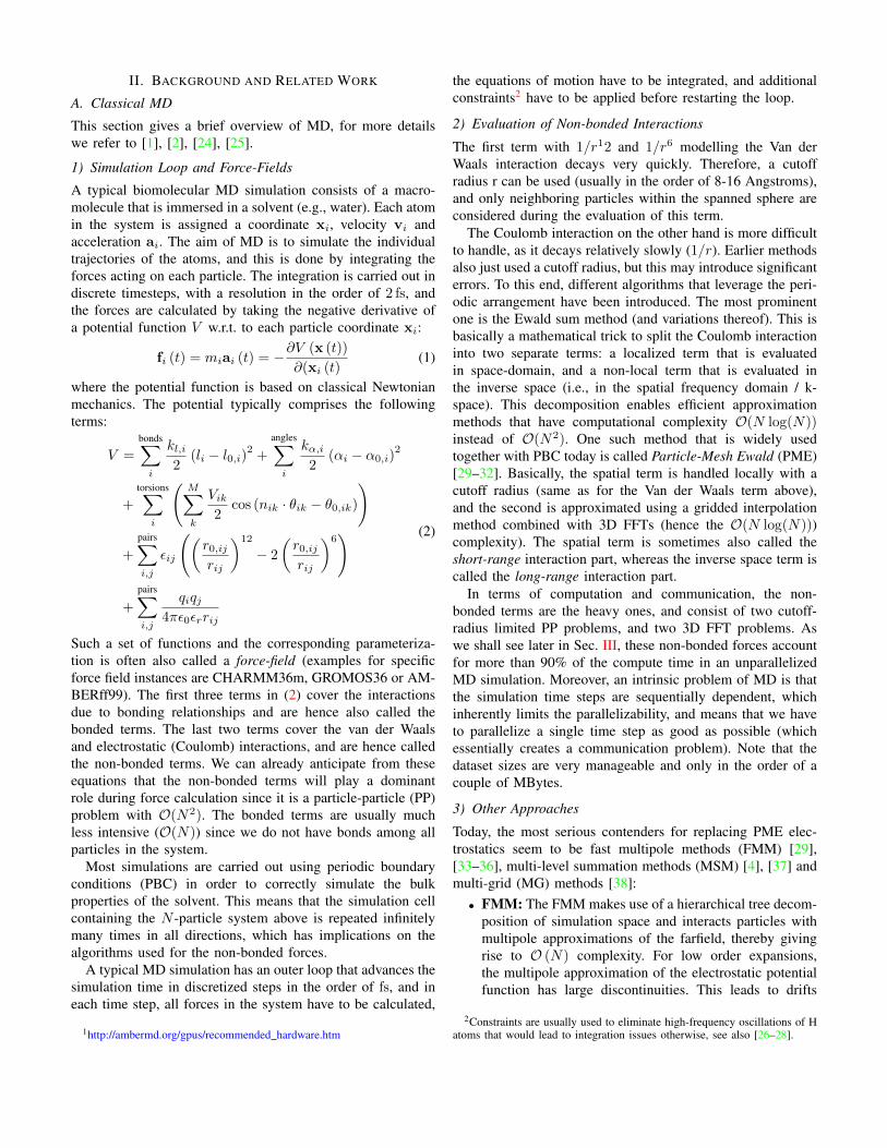
TABLE ITEST NODES USED FOR BENCHMARKING. THE P[2,3].[2,8,16]XLARGE

NODES ARE COMPUTE INSTANCES AVAILABLE ON AWS.

Node Name CPU (GHz) vCPUs† GPU Config

Sassauna E5-2640v4 (2.4) 40 4×GTX1080TiP2.2xlarge E5-2686v4 (2.3) 8 1×K80‡

P2.8xlarge E5-2686v4 (2.3) 32 4×K80‡

P2.16xlarge E5-2686v4 (2.3) 64 8×K80‡

P3.2xlarge E5-2686v4 (2.3) 8 1×V100 SMX2†

The number of vCPUs (virtual CPUs) corresponds to theamount of concurrent threads.

‡The K80 is a dual GPU card,

so the effective number of GPUs is double the listed number.

many implementation details), it seems to be reasonable thatsuch an approach yields good results in this setting. The FFTis quite a regular algorithm which can be well described withOpenCL, and the Altera FFT IP’s incur some overhead due tointernal buffering, interfaces, etc. which are not needed.

On the other hand, Saunullah et al. [50] attempt to useOpenCL to design the same PP interaction pipeline that theydeveloped with HDL in an earlier papers [14], [20], [21]. Theirconclusion is that for such a highly tuned datapath OpenCLdoes not provide competitive results (”...the OpenCL versionsare dramatically less efficient, with the Verilog design fittingfrom 3.5× to 7× more logic.”). The work by Cong et al. [23]is a similar study that investigates a Xilinx HLS flow for thesame PP interaction module. Their experiments reveal that partof the inefficiency of HLS for this particular module is the factthat HLS tools currently have difficulties producing efficientresults for datapaths with dynamic data flow behavior whereconditional execution exists within a processing element. Theirsolution is to describe certain parts critical for dynamic dataflow in HDL, and generate the remaining subblocks of thedatapath using HLS.

So based on our own experience and the above literature,we can say that OpenCL or HLS can increase productivity, andyield good results for algorithms that can be described well andthat have regular compute patterns (e.g., systolic dataflow, nofeedback loops, no dynamic control behavior). But for designsthat are difficult to describe and tune with OpenCL such asparts of the force-pipeline a highly tuned HDL implementationturns out to be more efficient. An interesting design approachis to use a mix between both methodologies, leveragingHLS (and its automated verification functionality) for smalldatapath subblocks that are then connected and orchestratedusing an HDL wrapper.

E. Vendor and Market Overview

Several well known high-performance software packages comefrom the academic sector and some of them like GROMACS[52–54] and LAMMPS [55] are released freely under open-source licences. Others like such as AMBER [56], NAMD[57] and CHARMM [58] provide reduced or free academiclicenses and require full licensing for commercial purposes.

Besides these codes originating from academia, there area couple of companies that develop and sell MD simulation

software such as Biovia from Dassault Systemes, AceMDfrom Acellera Ltd [59], Yasara [5], and Desmond from ShawResearch LLC [60] to name a few (see this market reportfor more info [61]). Some of the main differentiators of thesecommercial software packages comprise:

• Workflow integration and collaborative tools (e.g., Das-sault Systems),

• Better visualization and GUI integration (e.g., DassaultSystems, Yasara),

• Performance tweaks for workstation systems (e.g.,Yasara, Acellera),

• Extreme scalability on clusters (e.g., Shaw Research),• Costumer support and consulting options (all of them).

In terms of infrastructure, some companies sell applicationcertified workstations and server blades, such as Exxact-Corp5 (GROMACS and AMBER workstations) and Acellera(AceMD MetroCubo)6. Another interesting trend in this fieldseem to be cloud services [61], [62]. E.g., Acellera AceMDhas built-in support for Amazon Web Services (AWS), thatallows users to conveniently outsource simulation runs with asingle command. The advantage of such cloud solutions arescalability and low up-front costs, which can be attractive forsmall labs and/or labs that have large variations in workload.Otherwise on-prem solutions can be more cost-effective.

The overall market however can be considered a niche mar-ket, since there are only a few 1000 to 10’000 users worldwidethat use such specialized software packages. According toGoldbeck et al. [63], the overall spending on scientific softwareis in the order of 0.1% of the total sector R&D spending,which would amount to roughly 100M$ in pharma/biotech and50M$ in the chemicals/materials industry in Europe. Now thisis an estimate for the total spending, so for a specific softwarepackage the market size will only be a fraction of that. Soassuming a share in the order of 1% we can estimate that themarket for a specific software package is likely in the orderof several 100k$ to a few M$.

In this report, we use AMBER and GROMACS as bench-mark baselines, since these provide very competitive runtimeson single-node systems and are widely used in the community.In addition to on-prem solutions, we also consider cloudinfrastructure, since FPGAs have recently become available asa service (FaaS), in the form of the AWS F1 instance7. EdicoGenomics8 is an example for a company that successfully usesF1 instances to accelerate Genome sequencing.

III. SOFTWARE BENCHMARKS

In this section we assess the performance of two widelyused GPU-accelerated MD packages using three differentbenchmarks and recent hardware. This is done to get a solidbaseline for the comparisons with the FPGA performanceestimates in Sec. IV.

5https://www.exxactcorp.com/GROMACS-Certified-GPU-Systems6https://www.acellera.com/7https://aws.amazon.com/ec2/instance-types/f1/8http://edicogenome.com/

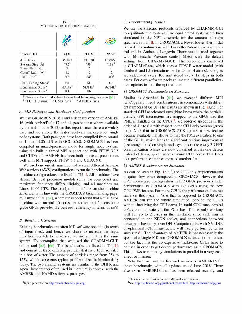
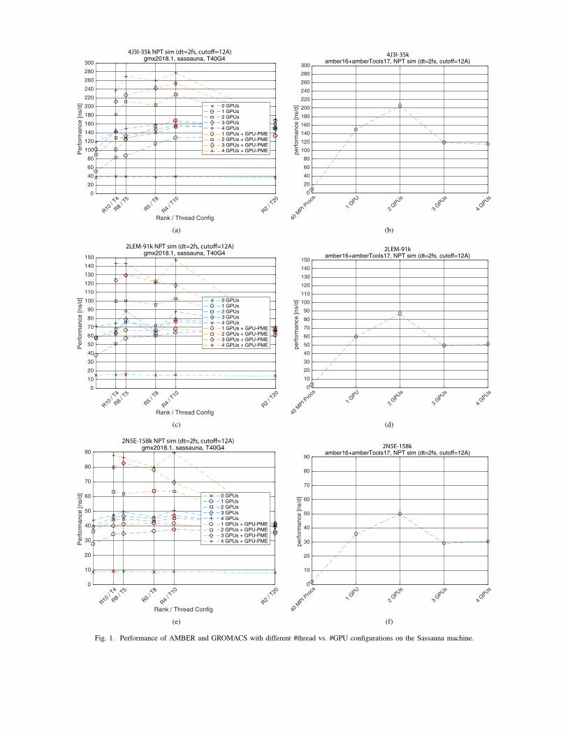
TABLE IIMD SYSTEMS USED FOR BENCHMARKING.

Protein ID 4J3I 2LEM 2N5E

# Particles 35’022 91’030 157’853System Size [A] ˜723 ˜993 ˜1193

Time Step [fs] 2 2 2Cutoff Radii [A]† 12 12 12PME Grid† 603 843 1003

PME Tuning Stepsg 6k 6k 6kBenchmark Stepsg 9k/14k‡ 9k/14k‡ 9k/14k‡

Benchmark Stepsa 10k 10k 10k† These are the initial values before load balancing, see also [64].‡ CPU/GPU runs. g GMX runs. a AMBER runs.

A. MD Packages and Hardware Configuration

We use GROMACS 2018.1 and a licensed version of AMBER16 (with AmberTools 17 and all patches that where availableby the end of June 2018) in this report, since these are widelyused and are among the fastest software packages for singlenode systems. Both packages have been compiled from scratchon Linux 14.06 LTS with GCC 5.5.0. GROMACS has beencompiled in mixed-precision mode for single node systemsusing the built-in thread-MPI support and with FFTW 3.3.5and CUDA 9.2. AMBER has been built in mixed-precision aswell with MPI support, FFTW 3.3 and CUDA 9.0.

We used one on-site machine and several different AmazonWebservices (AWS) configurations to run the benchmarks. Themachine configurations are listed in Tbl. I. All machines havealmost identical processor models (only the core count andmaximum frequency differs slightly), and all machines ranLinux 14.06 LTS. The configuration of the on-site machineSassauna is in line with the GROMACS benchmarking paperby Kutzner et al. [64], where it has been found that a dual Xeonmachine with around 10 cores per socket and 2-4 customergrade GPUs provides the best cost-efficiency in terms of ns/$.

B. Benchmark Systems

Existing benchmarks are often MD software specific (in termsof input files), and hence we chose to recreate the inputfiles from scratch to make sure we are simulating the samesystem. To accomplish that we used the CHARMM-GUI9

online tool [65], [66]. The benchmarks are listed in Tbl. II,and consist of three different proteins that have been solvatedin a box of water. The amount of particles range from 35k to157k, which represents typical problem sizes in biochemistrytoday. The two smaller systems are similar to the DHFR andApoa1 benchmarks often used in literature in context with theAMBER and NAMD software packages.

9Input generator on http://www.charmm-gui.org/

C. Benchmarking Results

We use the standard protocols provided by CHARMM-GUIto equilibrate the systems. The equilibrated systems are thensimulated in the NPT ensemble for the amount of stepsspecified in Tbl. II. In GROMACS, a Nose-Hoover thermostatis used in combination with Parinello-Rahman pressure con-trol and in Amber, a Langevin Thermostat is used togetherwith Montecarlo Pressure control (these were the defaultsettings from CHARMM-GUI). The force-fields employedis CHARMM36m, which uses a TIPS3P water model (withCoulomb and LJ interactions on the O and H atoms). Energiesare calculated every 100 and stored every 1k steps in bothcases. For each software package, we run different paralleliza-tion options to find the optimal one.

1) GROMACS Benchmarks on Sassauna

Similar as described in [64], we sweeped different MPIrank/openmp thread combinations, in combination with differ-ent numbers of GPUs. The results are shown in Fig. 1a,c,e. Forstandard GPU accelerated runs (blue lines) where the particle-particle (PP) interactions are mapped to the GPUs and thePME is handled on the CPUs10, we observe speedups in theorder of 4× to 6× with respect to the CPU-only version (greenline). Note that in GROMACS 2018 update, a new featurebecame available that allows to map the PME evaluation to oneof the GPUs, which leads to significant runtime improvement(see orange lines) on single-node systems as the costly 3D FFTcommunication phases are now contained within one deviceinstead of being spread accross many CPU cores. This leadsto a performance improvement of another 2×.

2) AMBER Benchmarks on Sassauna

As can be seen in Fig. 1b,d,f, the CPU-only implementationis quite slow when compared to GROMACS. However, theGPU accelerated configuration with 2 GPUs provides similarperformance as GROMACS with 1-2 GPUs using the newGPU PME feature. For more GPUs, the performance does notscale on this system. Note that as opposed to GROMACS,AMBER can run the whole simulation loop on the GPUswithout involving the CPU cores. In multi-GPU runs, severalGPUs communicate via the PCIe bus. This is only workingwell for up to 2 cards in this machine, since each pair isconnected to one XEON socket, and connections bettweenthese pairs have to go over QPI. Compute nodes with NVLINKor optimized PCIe infrastructure will likely perform better onsuch runs11. The advantage of AMBER is not necessarily thespeed of a single MD run (GROMACS is faster in that case),but the fact that the no expensive multi-core CPUs have tobe used in order to get decent performance as in GROMACS.This allows to run many simulations in parallel in a very cost-effective manner.

Note that we used the licensed version of AMBER16 forthese benchmarks with all updates as of June 2018. Therealso exists AMBER18 that has been released recently, and

10This is done without separate PME ranks in this case.11See http://ambermd.org/gpus/benchmarks.htm, http://ambermd.org/gpus

R10 /

T4

R8 / T

5

R5 / T

8

R4 / T

10

R2 / T

20

Rank / Thread Config

0

20

40

60

80

100

120

140

160

180

200

220

240

260

280

300

Per

form

ance

[ns/

d]

4J3I-35k NPT sim (dt=2fs, cuto�=12A) gmx2018.1, sassauna, T40G4

0 GPUs1 GPUs2 GPUs3 GPUs4 GPUs1 GPUs + GPU-PME2 GPUs + GPU-PME3 GPUs + GPU-PME4 GPUs + GPU-PME

(a)

40 M

PI Pro

cs

1 GPU

2 GPUs

3 GPUs

4 GPUs

0

20

40

60

80

100

120

140

160

180

200

220

240

260

280

300

perf

orm

ance

[ns/

d]

4J3I-35k amber16+amberTools17, NPT sim (dt=2fs, cutoff=12A)

(b)

R10 /

T4

R8 / T

5

R5 / T

8

R4 / T

10

R2 / T

20

Rank / Thread Config

0

10

20

30

40

50

60

70

80

90

100

110

120

130

140

150

Per

form

ance

[ns/

d]

2LEM-91k NPT sim (dt=2fs, cuto�=12A) gmx2018.1, sassauna, T40G4

0 GPUs1 GPUs2 GPUs3 GPUs4 GPUs1 GPUs + GPU-PME2 GPUs + GPU-PME3 GPUs + GPU-PME4 GPUs + GPU-PME

(c)

40 M

PI Pro

cs

1 GPU

2 GPUs

3 GPUs

4 GPUs

0

10

20

30

40

50

60

70

80

90

100

110

120

130

140

150

perf

orm

ance

[ns/

d]

2LEM-91k amber16+amberTools17, NPT sim (dt=2fs, cutoff=12A)

(d)

R10 /

T4

R8 / T

5

R5 / T

8

R4 / T

10

R2 / T

20

Rank / Thread Config

0

10

20

30

40

50

60

70

80

90

Per

form

ance

[ns/

d]

2N5E-158k NPT sim (dt=2fs, cuto�=12A) gmx2018.1, sassauna, T40G4

0 GPUs1 GPUs2 GPUs3 GPUs4 GPUs1 GPUs + GPU-PME2 GPUs + GPU-PME3 GPUs + GPU-PME4 GPUs + GPU-PME

(e)

40 M

PI Pro

cs

1 GPU

2 GPUs

3 GPUs

4 GPUs

0

10

20

30

40

50

60

70

80

90

perf

orm

ance

[ns/

d]

2N5E-158k amber16+amberTools17, NPT sim (dt=2fs, cutoff=12A)

(f)

Fig. 1. Performance of AMBER and GROMACS with different #thread vs. #GPU configurations on the Sassauna machine.

sass

auna

, 2xla

rge

sass

auna

, 8xla

rge

sass

auna

, T40

G4

awsP

3.2x

large

, 2xla

rge

awsP

2.16

xlarg

e, 2

xlarg

e

awsP

2.16

xlarg

e, 8

xlarg

e

awsP

2.16

xlarg

e, 1

6xlar

ge0

20

40

60

80

100

120

140

160

180

200

220

240

260

280

300pe

rfor

man

ce [n

s/d]

4J3I-35k gmx2018.1, NPT sim (dt=2fs, cutoff=12A)

(a)

sass

auna

, 2xla

rge

sass

auna

, 8xla

rge

sass

auna

, T40

G4

awsP

3.2x

large

, 2xla

rge

awsP

2.16

xlarg

e, 2

xlarg

e

awsP

2.16

xlarg

e, 8

xlarg

e

awsP

2.16

xlarg

e, 1

6xlar

ge0

20

40

60

80

100

120

140

perf

orm

ance

[ns/

d]

2LEM-91k gmx2018.1, NPT sim (dt=2fs, cutoff=12A)

(b)

sass

auna

, 2xla

rge

sass

auna

, 8xla

rge

sass

auna

, T40

G4

awsP

3.2x

large

, 2xla

rge

0

20

40

60

80

perf

orm

ance

[ns/

d]

2N5E-158k gmx2018.1, NPT sim (dt=2fs, cutoff=12A)

(c)

Fig. 2. Comparison of the performance of GROMACS on different AWS instances and the corresponding configurations on the Sassauna machine. The largestbenchmark has not been run on AWS due to long benchmark runtimes.

that likely includes further optimizations for the Pascal andVolta generation GPUs.

3) GROMACS Benchmarks on AWS

As mentioned in the introduction, cloud infrastructure/softwareservices (IaaS/SaaS) are interesting alternatives to on-sitesolutions. Hence, we also benchmark a few AWS instancesin order to be able to include them in the performance costcomparison later on in Sec. IV.

At the time of writing, the demand for P3 instances withV100 SMX2 cards was extremely high, and hence we onlygot access to one 2xlarge instance with one GPU. As such, theperformance improvements for multi-GPU runs with V100’shas to be extrapolated from these measurements. As we canobserve in Fig. 2 the improvement is in the order of 20% withrespect to the GTX1080Ti for the larger benchmarks. Thisimprovement seems to be reasonable, since the raw increase inFLOP/s is around 35%. We can also see that the P2 instanceswith K80 GPUs are significantly slower than the P3 instanceor Sassauna.

4) GROMACS Breakdown of Simulation Loop

The walltime breakdown for the three different benchmarks isshown in Tbl. III in % for three different cases: single threaded(CPU-only), multi-threaded with PME on CPUs, and multi-threaded with both PP interactions and PME on GPUs.

The walltime breakdown for the single-threaded case isshows the well-known picture: the compute time is mainlydominated by non-bonded force evaluations, which accountsfor more than 96%, including PME. The force time alsoincludes bonded forces in this case, but the fraction is in-significant compared to the non-bonded part.

In the multi-threaded case with PP interactions on the GPU,the picture already changes quite a bit. The runtime of the PPinteraction kernels is not visible since they are executed inparallel to the CPU code, for which the walltime accountingis performed. The breakdown is a bit more difficult to read,but we see that PME starts to become the dominant factor(more than 50%)..

In the third case, we note that other parts besides the PPinteractions and PME are starting to become significant aswell. In particular the operations that cannot be overlappedwith the accelerated PP and PME calculations (such as domaindecomposition, reduction operations, trajectory sampling, in-tegration, global energy communication) start to amount fora significant percentage of overall walltime (around 25% inthis benchmarks). As we shall see in Sec. IV on hardwareperformance estimates, this inherently limits the maximumacceleration that can be achieved by using a co-processorsolution. This issue is not exclusive to GROMACS, and hasalso been noted, e.g., in [67] with NAMD.

It is worth noting that the constraints step is required to keephigh-frequency oscillations of bonds involving light atoms(H) under control. Otherwise, significantly smaller timestepsthan the currently employed 2 fs have to be employed inorder to ensure correct integration and prevent the simulationfrom blowing up. These constraints are implemented using acombination of efficient parallel algorithms in GROMACS (P-LINCS for general bonds [26], [27], analytic SETTLE [28] forwater molecules).

IV. PERFORMANCE ESTIMATIONS AND COMPARISONS

In this section, we estimate the performance of FPGA ac-celerated systems, compare them with GPU-based solutions

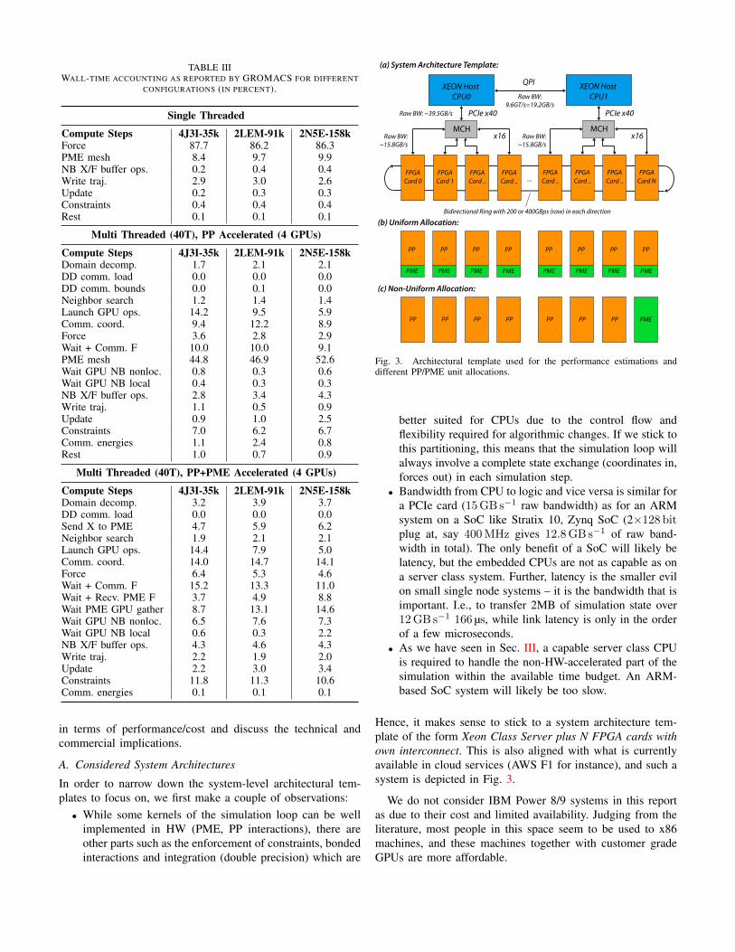
TABLE IIIWALL-TIME ACCOUNTING AS REPORTED BY GROMACS FOR DIFFERENT

CONFIGURATIONS (IN PERCENT).

Single Threaded

Compute Steps 4J3I-35k 2LEM-91k 2N5E-158kForce 87.7 86.2 86.3PME mesh 8.4 9.7 9.9NB X/F buffer ops. 0.2 0.4 0.4Write traj. 2.9 3.0 2.6Update 0.2 0.3 0.3Constraints 0.4 0.4 0.4Rest 0.1 0.1 0.1

Multi Threaded (40T), PP Accelerated (4 GPUs)

Compute Steps 4J3I-35k 2LEM-91k 2N5E-158kDomain decomp. 1.7 2.1 2.1DD comm. load 0.0 0.0 0.0DD comm. bounds 0.0 0.1 0.0Neighbor search 1.2 1.4 1.4Launch GPU ops. 14.2 9.5 5.9Comm. coord. 9.4 12.2 8.9Force 3.6 2.8 2.9Wait + Comm. F 10.0 10.0 9.1PME mesh 44.8 46.9 52.6Wait GPU NB nonloc. 0.8 0.3 0.6Wait GPU NB local 0.4 0.3 0.3NB X/F buffer ops. 2.8 3.4 4.3Write traj. 1.1 0.5 0.9Update 0.9 1.0 2.5Constraints 7.0 6.2 6.7Comm. energies 1.1 2.4 0.8Rest 1.0 0.7 0.9

Multi Threaded (40T), PP+PME Accelerated (4 GPUs)

Compute Steps 4J3I-35k 2LEM-91k 2N5E-158kDomain decomp. 3.2 3.9 3.7DD comm. load 0.0 0.0 0.0Send X to PME 4.7 5.9 6.2Neighbor search 1.9 2.1 2.1Launch GPU ops. 14.4 7.9 5.0Comm. coord. 14.0 14.7 14.1Force 6.4 5.3 4.6Wait + Comm. F 15.2 13.3 11.0Wait + Recv. PME F 3.7 4.9 8.8Wait PME GPU gather 8.7 13.1 14.6Wait GPU NB nonloc. 6.5 7.6 7.3Wait GPU NB local 0.6 0.3 2.2NB X/F buffer ops. 4.3 4.6 4.3Write traj. 2.2 1.9 2.0Update 2.2 3.0 3.4Constraints 11.8 11.3 10.6Comm. energies 0.1 0.1 0.1

in terms of performance/cost and discuss the technical andcommercial implications.

A. Considered System Architectures

In order to narrow down the system-level architectural tem-plates to focus on, we first make a couple of observations:• While some kernels of the simulation loop can be well

implemented in HW (PME, PP interactions), there areother parts such as the enforcement of constraints, bondedinteractions and integration (double precision) which are

MCH

XEON Host CPU0

FPGACard 0

FPGACard 1

FPGACard ..

FPGACard ..

MCH

XEON Host CPU1

FPGACard ..

FPGACard ..

FPGACard ..

FPGACard N

QPI

PCIe x40 PCIe x40

x16

Raw BW: ~39.5GB/s

Raw BW:~15.8GB/s

x16Raw BW:~15.8GB/s

Raw BW:9.6GT/s=19.2GB/s

Bidirectional Ring with 200 or 400GBps (raw) in each direction

(b) Uniform Allocation:

(c) Non-Uniform Allocation:

PME PME PME PME PME PME PME PME

PME

PP PP PP PP PP PP PP PP

PP PP PP PP PP PP PP

(a) System Architecture Template:

...

Fig. 3. Architectural template used for the performance estimations anddifferent PP/PME unit allocations.

better suited for CPUs due to the control flow andflexibility required for algorithmic changes. If we stick tothis partitioning, this means that the simulation loop willalways involve a complete state exchange (coordinates in,forces out) in each simulation step.

• Bandwidth from CPU to logic and vice versa is similar fora PCIe card (15GB s−1 raw bandwidth) as for an ARMsystem on a SoC like Stratix 10, Zynq SoC (2×128 bitplug at, say 400MHz gives 12.8GB s−1 of raw band-width in total). The only benefit of a SoC will likely belatency, but the embedded CPUs are not as capable as ona server class system. Further, latency is the smaller evilon small single node systems – it is the bandwidth that isimportant. I.e., to transfer 2MB of simulation state over12GB s−1 166 µs, while link latency is only in the orderof a few microseconds.

• As we have seen in Sec. III, a capable server class CPUis required to handle the non-HW-accelerated part of thesimulation within the available time budget. An ARM-based SoC system will likely be too slow.

Hence, it makes sense to stick to a system architecture tem-plate of the form Xeon Class Server plus N FPGA cards withown interconnect. This is also aligned with what is currentlyavailable in cloud services (AWS F1 for instance), and such asystem is depicted in Fig. 3.

We do not consider IBM Power 8/9 systems in this reportas due to their cost and limited availability. Judging from theliterature, most people in this space seem to be used to x86machines, and these machines together with customer gradeGPUs are more affordable.

B. Estimated System Components

As explained before, we assume the architectural templateshown in Fig. 3a). For the FPGA cards, we base the resourceand performance estimates on reported values in literature, asexplained below.

1) Interconnects

The assumed architectural template consists of two XEONhost CPUs that can host a maximum of 4 cards at full x16PCIe bandwidth, or 8 cards at x8 bandwidth. For the PCIelink efficiency (framing and other overheads), we assume abandwidth efficiency of 75% and a latency of 10 µs. Furtherwe assume that the FPGA cards are interconnected with abidirectional ring. This is readily possible due to the highamount of transceivers available on todays high-end FPGAs.In fact, almost every PCIe FPGA card features at least oneQSFP port. As explained later, the targeted FPGA platformseither provide two or four QSFP28 cages, allowing for rawring bandwidths of 200 or 200-400Gbit. The assumed link ef-ficiency is 85% including framing and packetizing overheads,and a link latency of 0.5 µs is assumed.

2) PP Interaction Pipelines

We base our estimates on the PP interaction pipeline by M.Herbordt’s group [20], [21] that employs particle filters thatgenerate the neighbor lists on-the-fly. This architecture is wellsuited for hardware implementations, and does not require asmuch memory as an implementation with explicit neighbor-lists. The employed arithmetic is a mix between fixed-pointand single-precision floating-point, and has been optimized forFPGAs. The employed domain decomposition is an optimizedvariant of the half shell method. Better methods with lessinter-cell communication volume exist (e.g., neutral territoryand mid-point methods [60]), but these are likely to showtheir benefits only in the highly scaled regime (which isnot the scope of this evaluation). According to the resultsof Herbordt et al., the preferred design employs first-orderinterpolation with piecewise polynomials, and this designamounts to around 14.5k ALMs and 82 DSP multipliers ona Stratix IV (including filters, LJ and Coulomb datapath,distribution and accumulation logic). We estimate the neededamount of memory separately as described further below.

The PP interaction pipelines can calculate one interactionper cycle. In terms of utilization, the authors reported that itis possible to achieve relatively high percentages in the orderof 95% by properly mapping the particles to the filters andLJ/Coulomb force datapaths. However, since in our evaluationwe deal with many more parallel pipelines (several 100 insteadof several tens), we assume a slightly reduced utilization of80% to account for potential imbalances.

The required RAM resources have been estimated by as-suming that each particle position entry requires three 32 bitcoordinate entries plus one 32 bit entry holding metadata likeatom ID and type (we assume that atom specific LJ interactionvalues and charge parameterizations can be compiled intoROMs and indexed by these atom type IDs at runtime). Theparticle force accumulation entries are assumed to comprise

TABLE IVASSUMED COSTS FOR THE COMPARISON. EQUIPMENT AND SOFTWARE

PACKAGES ARE AMORTIZED OVER 5 YEARS (STRAIGHT LINE), AND THEELECTRICITY IS ASSUMED TO COST 0.1$ PER KWH. FURTHER, FOR EACH

ON-SITE SOLUTION WE DOUBLE THE ELECTRICITY COST IN ORDER TOACCOUNT FOR COOLING.

Component Cost [$] [kW] Details

Server with 4×PCIe† 8’000 0.45 Dual E5-2640v4Server with 8×PCIe† 11’000 0.45 Dual E5-2640v4P100 6’000 0.25 Pascal GenerationGTX1080Ti 800 0.25 Pascal GenerationTITAN-XP 1’350 0.25 Pascal GenerationV100 SMX2 10’000 0.25 Volta GenerationTITAN-V 3’600 0.25 Volta GenerationVCU1525 (VU9P) 4’500 0.25 200GBit RingXUPP3R (VU9P) 10’000 0.25 400GBit RingXUPP3R (VU13P) 15’000 0.25 400GBit RingDE10-PRO (GX2800) 15’000 0.25 400GBit Ring

p3.2xlarge‡ 3.305 – 1×V100p3.8xlarge‡ 13.22 – 4×V100f1.2xlarge‡ 1.815 – 1×XUPP3R (VU9P)∗

f1.16xlarge‡ 14.52 – 8×XUPP3R (VU9P)∗

Amber License+ 20’000/4 – Commercial, Site† Assuming the same dual Xeon configuration of the Sassaunanode used for benchmarking. ‡ For the AWS instances, theprices are per hour. + The Amber license is a site license.We assume here for simplicity that a site consists of 4 nodesto amortize the license cost. ∗ Or a similar FPGA card thatprovides up to 400Gbit ring interconnection capability.

three 32 bit values. The estimation for memory usage includesall interpolator lookup tables, atom property ROMs, all posi-tion+metadata entries and private accumulation buffers of thePP interaction pipelines.

3) PME Unit

Herbordt’s group demonstrated as well that it is possible tofit a 3D FFT unit with 643 grid points onto recent FPGAs[18], [19]. The dominant factor here are the 1D FFT macrosprovided by the FPGA vendors. Hence, we use the complexityof these vendor provided macros to estimate the resources forthe 3D FFT part. Since our FFTs sizes are in the order of843 grid points, we assume that the resource consumptionis similar to 128-point FFT macros, i.e., 5k LUT, 32 DSPmultipliers and 16kBit memory on a VUP FPGA12. Thelatency corresponds to the amount of samples to be calculated.

For the particle-to-grid and grid-to-particle interpolators,we use the results reported in [16], where an optimizedsingle-cycle datapath is designed and implemented. One suchunit requires 51k ALMs 192 DSP blocks (= 2 × 192 DSPmultipliers) on a Stratix V FPGA. Further, we assume that thisdesign can be optimized such that the same interpolators canbe used for both interpolation directions, as well as the PMEsolution step in the frequency domain that entails a point-wisemultiplication with pre-computed constants.

12Note that these implementations likely use a Cooley-Tukey FFT that canonly be used for lengths that are powers of two. In practice, a split-radix FFTwould be required to handle other FFT lengths.

TABLE VCONSIDERED FPGA CONFIGURATIONS (EACH LISTED SOLUTION EMPLOYS 7 PP FPGA CARDS AND 1 PME FPGA CARD).

Evaluated Configurations

Platform/Board VCU1525 XUPP3R XUPP3R DE10 Pro f1.x16large‡FPGA VU9P VU9P VU13P 1SGX280 VU9P

Cutoff [A]† 12.6 12.3 12.6 12.0 12.0PME Grid† 803 823 803 843 843

vCPUs 40 40 40 40 64Core Freq. [MHz] 400 400 400 700 400Ring BW (raw/eff) [GBit] 200/170§ 400/340§ 400/340§ 400/340§ 400/340§

PCIe BW (raw/eff) [GBit] 63/54+ 63/54+ 63/54+ 63/54+ 63/54+

PP Pipelines / FPGA 66 66 108 42 58Grid Interpolators / FPGA 10 10 18 6 9Mixed Radix FFT Units / FPGA 64 64 96 64 64

Estimated Resource UtilizationPP FPGA Logic [kLUT] 887.9 (75.1%) 885.8 (74.9%) 1452.9 (84.1%) 701.0 (75.1%) 782.1 (85.6%)PP FPGA DSP 2706.0 (39.6%) 2706.0 (39.6%) 4428.0 (36.0%) 1722.0 (14.9%) 2378.0 (42.2%)PP FPGA Memory [MBit] 78.3 (23.0%) 78.3 (23.0%) 124.4 (27.4%) 46.7 (20.4%) 62.2 (36.3%)

PME FPGA Logic [kLUT] 846.9 (71.6%) 846.9 (71.6%) 1428.4 (82.7%) 711.3 (76.2%) 794.2 (86.9%)PME FPGA DSPs 5888.0 (86.1%) 5888.0 (86.1%) 9984.0 (81.2%) 4352.0 (37.8%) 5504.0 (97.6%)PME FPGA Memory [MBit] 50.2 (14.7%) 54.0 (15.8%) 50.7 (11.2%) 57.9 (25.3%) 57.9 (33.8%)

Estimated Runtimes and PerformancePME + H2D Transfers[µs] 274.4 250.9 168.1 196.5 269.0PP + H2D Transfers[µs] 268.4 250.6 168.1 210.4 264.1PP/PME + D2H Transfers [µs] 307.5 284.0 201.2 243.5 302.1SW Overheads [µs] 280.0 280.0 280.0 280.0 175.0

Total HW+SW [µs] 587.5 564.0 481.2 523.5 477.1Performance [ns/d] 294.1 306.4 359.1 330.1 362.2†We employ a similar load balancing mechanism as GROMACs between PME and PP cards.‡ The maximum available resources are reduced in this case due to the AWS shell infrastructure (see text for more details).+ We assume a PCIe link efficiency of 75%, and since we use 8 PCIe cards only half the 16x bandwidth is available per FPGA.§ Assuming a link efficiency of 85% for the ring interconnect.

4) Resource Allocation

In terms of allocation of PME and PP units to acceleratorboards it seems natural to uniformly distribute them as illus-trated in Fig. 3b). The advantage of this allocation is scalabilityof compute resources. However, the communication pattern ofthe two 3D FFT passes in PME leads to high communicationvolume between these distributed PME units, and hence it hasbeen found that a contraction in the PME calculation can leadto better performance [68]. E.g., for highly parallel scenariosGROMACS supports the use of fewer separate MPI ranks [53].Further, an additional optimization for single node systemshas been added in the newest GROMACS release where thePME calculation can be allocated to one GPU. AMBER movedto single GPU implementations already a while ago to solvethis communication issue. Hence, we do not consider uniformallocation, but the non-uniform allocation shown in Fig. 3c).

5) Schedule

The computation schedule follows a relatively simple repeti-tive pattern. In each iteration, all MPI processes on the hostpush the particle coordinates and meta-information down tothe FPGA card using bulk DMA transfers, thereby utilizing thefull effectively available PCIe bandwidth. Computation on the

FPGA side can be largely overlapped with the PCIe transfers,since we can start computing PP interactions already with asmall part of the simulation volume. Further, the coordinatesand meta data can be gathered and transferred to the PME cardon-the-fly (via the ring interconnect), and the grid interpolatorscan start with particle-to-grid interpolation. As soon as thecomplete simulation volume has been transferred, the PP cardsexchange the overlap regions required for PP interactions viathe ring. Once the inverse 3D FFT is complete, the grid-to-particle interpolation can be started and overlapped withthe scatter operation that transfers the forces back to theoriginating card. The forces are then accumulated within thePP interaction force buffers, and once all non-bonded forceshave been calculated, the results are copied back to the host.

C. FPGA Targets and Hardware Costs

In order to achieve the required performance, large datacentergrade FPGAs are required. In this report we target the XilinxVirtex UltraScale+ series, as well as the Intel Stratix 10 series,since at the time of writing, these represent the best FPGAtechnology that is available (or soon will be). On the Xilinxside, we identified the VU9P device as an ideal target as itis currently widely used and stable in production (this device

is also available in the AWS F1 instances). The roughly 50%larger VU13P device will soon reach stable production, aswell, and can be seen as the natural successor of the VU9Pdevice in the forthcoming years. On the Intel side, the onlyFPGA that can currently match the Virtex UltraScale+ devicesis the upcoming Stratix 10 series (the Arria 10 devices are toosmall). In particular, it seems that the 1SGX280 device willbe the equivalent of the VU9P in terms of adoption (severaldevelopment boards feature this device). However, we foundthat the availability of these devices is not yet guaranteed(especially for the H-Tile devices with fast transceivers), andwe can expect that stable products are likely not to going tobe introduced before next year.

In order to compare system level costs, we assume the pricesand power consumptions13 listed in Tbl. IV. For simplicity,we lump the costs for the optical modules together with thecorresponding FPGA boards (roughly 200$ per QSFP28 slot).Equipment and software packages are amortized over 5 years(straight line), and the electricity is assumed to cost 0.1$per kWh. Further, for each on-site solution we double theelectricity cost in order to account for cooling. No sales marginis added to the FPGA solutions in this comparison, but in acommercial setting this has to be accounted for as well.

D. Evaluated Configurations and Assumptions

We calculate our estimates for a system with N = 8 FPGAcards in the system (as discussed earlier, the PP interactionpipelines are allocated on 7 FPGAs, while 1 FPGA card isused for PME). These configurations are listed in Tbl. V.The amount of units (e.g. FFTs) listed in that table is perFPGA instance. We note that on these modern FPGAs, logicresources are the ones that are going to be critical. In orderto allow for enough headroom for additional infrastructuresuch as, e.g., Aurora and PCIe PHYs we target a LUT/ALMusage of 75% on the VU9P and 1SGX280 devices (both offera similar amount of logic resources). On the larger VU13Pdevices and AWS F1 instance, we target a higher utilizationin the order of 85%. This is possible since the VU13P offersaround 50% more logic resources than the VU9P, and on theAWS instance, the infrastructure is already included in theAWS F1 Shell that wraps the user logic14.

From test syntheses of an HDL design optimized for FPGAs(NTX cores from [69]) we found that operating frequencies upto 400MHz and 700MHz should be achievable on the VirtexUltraScale+ and Stratix 10 devices, respectively. From thesetest syntheses we also calculated logic conversion factors forthe LUTs and ALMs to derate the numbers reported for the3D FFT and PP cores in literature (shown in Tbl. VI).

13For more information on the FPGA boards, see also:http://www.hitechglobal.com/Boards/UltraScale+ X9QSFP28.htm,https://www.xilinx.com/products/boards-and-kits/vcu1525-p.html,https://www.bittware.com/fpga/xilinx/boards/xupp3r/,https://www.altera.com/solutions/partners/partner-profile/terasic-inc-/board/terasic-stratix-10-de10-pro-fpga-development-kit.html

14AWS uses partial reconfiguration, and the logic resources available in theuser partition amounts to 914k, 5640 DSPs, 3360 BRAMs and 400 URAMs,which corresponds to 77%, 82%, 78% and 42% of the resources available onthe VU9P.

TABLE VIDERATING FACTORS FOR DIFFERENT FPGA GENERATIONS. THE HIGHER

# ALMS ON THE STRATIX 10 DEVICE IS LIKELY DUE THE HIGHOPERATING FREQUENCY TARGETED.

Source / Target VUP [LUTs] Stratix 10 [ALMs]

Stratix IV [ALMs] 0.95 1.18Stratix V [ALMs] 1.04 1.29

For the estimations in this section, we consider the 91kproblem (2LEM) of the previous section, and assume a soft-ware overhead of 280 µs on 40 logical cores that can not beoverlapped with the force computations (this amounts to 25%of the overall walltime of a single step, see previous sectionon benchmarks). Note that we adjust the PME grid resolutionand PP interaction cutoffs to balance the load between thePP and PME cards at similar accuracy. This is analogous tothe PME load balancing procedure performed in GROMACSsimulation runs [64].

We also note that we do not explicitly account for potentialand virial calculations here as these are only carried out every100 steps in the considered benchmarks. The support for thesecalculations can be added to the hardware either by extendingthe force pipelines (this leads to a small increase in DSP sliceswhich are still abundantly available) or by reusing existinginterpolator infrastructure and repeated evaluation, leading toa decrease in performance of around 1%.

E. Results

The estimations for resources and timings are shown in Tbl. Vat the bottom. The highest performance is achieved by theVU13P and f1.16xlarge designs. In the first case this is dueto the high amount of logic resources on the VU13P and inthe second case, more CPU cores translate into lower softwareoverheads. In all cases we note that the non-hideable softwareoverheads (domain decomposition, integration, constraints,etc.) are either in similar in magnitude than the acceleratedPP and PME portions.

When comparing the VCU1525 and XUPP3R solutions withVU9P FPGAs, we can observe that the faster ring interconnectavailable with the more expensive XUPP3R does lead to asmall improvement in speed, but this is likely not worth theprice increase of around 2× in case of the VU9P. However,for the larger/faster VU13P and 1SGX280 FPGAs, the fasterring interconnect is desirable in order to match the bandwidthwith the increased throughput.

In order to better compare different solutions, we cast theseresults into a performance (ns/d) versus cost ($/h) and adddifferent operating points of GPU-accelerated solutions. Theperformance values for FPGA versions with less than eightcards have been derated from the 8 card solutions (assumingthat one of the cards now contains both the complete PMEunit and some PP interaction pipelines). The performancevalues for the GPU solutions employing 1-4×GTX1080Ti and1 V100 (on AWS) have been measured (see previous sectionon benchmarks). The remaining operating points have been

10-1

100

101

Cost [$/h]

102

103

Per

form

ance

[ns/

d]

4xV100

1xV100

2xVCU15251xp3.2xlarge

ideal

1xV100

4xTITAN-V

4xGTX1080Ti

2xGTX1080Ti

1xGTX1080Ti1xP100

1xTITAN-V

1xTITAN-XP1xGTX1080Ti

2xGTX1080Ti

4xVCU1525

8xVCU15258xXUPP3R-VU9P

8xXUPP3R-VU13P

8xDE10-PRO

1xp3.8xlarge

1xf1.2xlarge

1xf1.16xlarge

better

GMX18AMBER17FPGAAWSideal

Fig. 4. Comparison of the performance vs cost tradeoff of different FPGAand GPU-based solutions on the 2LEM-91k benchmark.

estimated using numbers from existing benchmarks15.The blue dots are all for GROMACS 2018, the green ones

for AMBER 16/17 and the orange ones for FPGA solutionsbased Virtex UltraScale+ and Stratix 10 FPGAs. On the rightside of the plot we have the AWS instances, and on the leftthe on-prem versions. The closer solutions are to the upper leftcorner of the plot, the better, and the diagonal lines representsame performance/cost. The red dot in the upper left cornershows the desirable performance/cost of an ideal solution thatdomain experts would consider commercially feasible.

F. Discussion

As can be observed in Fig. 4, systems employing con-sumer grade GTX1080Ti cards are clearly at the forefrontin terms of cost efficiency (slanted lines represent equalperformance/cost). And it should be noted that this efficiencyis bound to increase, since there seems to be a trend inmoving more computations or even the complete simulationloop onto the GPUs and have them communicate in a peer-to-peer fashion. AMBER already supports this, allowing toassemble very cost efficient desktop systems, since in that caseno expensive high-core-count CPUs are required anymore.This is not reflected in the plot above yet, as these costs havebeen calculated assuming a dual XEON (20 core) server.

We can also see that with FPGA solutions based on Ul-traScale+ and Stratix 10 devices there is not much to begained with respect to the GPU solutions. I.e., it is possibleto achieve speedups in the order of around 1.5× to 2×, butthe performance/cost ratio is similar to GPU solutions. Thisis a combination of two key factors: first, FPGAs prices arein the range of datacenter GPUs, which makes it difficult tocompete with consumer grade GPUs that offer very attractivesingle-precision FLOPS/$ ratios. And second, the amount of

15See http://ambermd.org/gpus/benchmarks.htm

remaining work that can not be overlapped with non-bondedforce computations starts to become dominant, thereby leadingto a saturation of the achievable speedup. For instance, inthe case of a system with 8 VU13P FPGAs, our estimatesindicate that the PP and PME calculations take less timethan the remaining non-hideable parts in software (200 µsversus 280 µs). Hence, we see that even a 4× speedup of thecalculation of the PP interactions and PME only leads to anapplication performance improvement of only 2×.

1) Commercial Feasibility

We have been in contact with domain experts and accordingto them, a new accelerator solution based on a differenttechnology than GPUs should offer at least 1 µs of simulationperformance at the cost of one high-end GPU in order to beperceived as a viable alternative (this ideal solution is indicatedwith a red dot in Fig. 4). Considering our results and thisdesirable target, it becomes evident that a FPGA co-processorsolution will likely not be commercially successful since amere 2× improvement in speed at similar cost efficiency doesnot represent a compelling value proposition for potential users(we have to keep in mind here that an FPGA solution willlikely be less flexible in terms of functionality than a GPU-based one). Instead, MD users will likely just run severalsimulations in parallel at somewhat lower speed and bettercost efficiency, e.g., to improve sampling statistics or to screenmultiple chemical compounds in parallel.

2) A Note on Algorithmic Improvements

We see that when targeting non-bonded interactions, archi-tectural specialization and current FPGA technology alonewill likely not be enough to get the needed improvement inspeed (with respect to GPU solutions), and some algorithmicinnovation will be needed as well (that is, unless FPGA pricesdrop over 10× the coming years, which is not very probable).The following points should however be kept in mind whendoing algorithmic work in this field:• This is a mathematical field, and people would like to

have error guarantees and bounds. Despite the fact thatit is very challenging to come up with an algorithm thatis better than SOA, it takes a long time until such a newmethod is established and accepted by the community.For example, variations of FMM and multi-level summa-tion methods (MSM) [4], [37] have been in developmentfor many years now, and they still not used on a regularbasis for production runs – even if they may have benefitsin some operating regions. One of the reasons for thisslow development and adoption is that it is difficultto find and introduce optimizations/approximations thatdo not introduce assumptions that violate physical lawsand eventually lead to erratic behavior. Further, it isdifficult to verify the correctness of a certain approachor implementation.

• It is likely that GPU-based solutions will benefit fromalgorithmic improvements, too (e.g., improvements of theintegration and constraints steps), and the implementationturn-around time is shorter for GPUs than for FPGAs.

• Machine-learning approaches are well suited for a certainclass of ab-initio potential evaluations (AIMD), and theyhave been shown to give quite impressive speedups inthat case. However, in pure classical MD, the force fieldsalready have a very simple and efficient functional form(basically polynomial expressions for classical mechan-ics), and contain far fewer parameters than, e.g., the ANI-1 NN potential [39]. It is currently unclear how such anNN-based approach could be used to accelerate potentialexpressions in classical MD simulations.

3) Other Hardware Acceleration Opportunities

ASIC integration of the non-bonded interaction pipelines couldbe a way of improving the performance with respect to FPGA-based solutions, but in the end this approach suffers thesame shortcomings as the FPGA co-processor solution, and inaddition the market does not seem to be big enough to justifythe development costs. Moving to fully integrated solutions ina similar fashion as this has been done in the Anton systemscan also lead to higher performance, but the design effort (andinvolved risks) are quite large and hence difficult to justify. Sofar, Anton-1/2 SoCs have been the only successful chips builtin this fashion. MDGRAPE-4, which is the only other SoC-based system, seems to be fizzled out as there has been noupdate on the project for 4 years (the last publication [7] isfrom 2014). Another fact that has to be kept in mind is thatthere are several patent applications and granted patents [70–73] protecting features of the Anton-type SoCs, which couldcomplicate commercial exploitation of such a solution.

Considering the difficulties mentioned above, it becomesclear that different approaches for leveraging FPGAs shouldbe considered. It could make sense to turn towards scaleddatacenter solutions and look into hybrid solutions that lever-age FPGAs as near-network accelerators (similar as this hasbeen done in Catapult-I/II [47], [48], or applications suchas networking filtering, high-frequency trading, etc). I.e., wecould use FPGAs to complement multi-node GPU systems inorder to improve the scalability of such systems. Consider forinstance the scaling behavior of GPU-accelerated GROMACSruns on the Hydra supercomputer (Max Planck ComputingCentre, 20-core Ivy Bridge nodes with 2xK20X and FDR-14)in Fig. 5. We can observe the well-known hard-scaling issuefor typical problem sizes (top 2 curves, 81k atoms). Problemswith several millions of atoms (lower 4 curves) are often usedfor benchmarking, but they do not represent common everydayproblems. What is interesting to note is that GPU acceleratedproblems with ¡100k atoms often reach their 50% scaling limitvery quickly at around 8 nodes - and this is something thatcan be observed on other clusters, too (see [64], for example).From what can be read in literature this scaling bottleneck ismainly due to PME and global communication phases.

So it is likely that a network accelerator could be used toameliorate this scaling bottleneck by bypassing the standardInfiniBand interconnects and the MPI software stack, andby providing a dedicated secondary network with functionalcapabilities tailored towards PME and global communication(e.g. for energies and virials) and even integration/constraints

Fig. 5. GROMACS scaling on HYDRA (Max Planck Computing Centre),reproduced from [53].

handling. Possible arrangements could be 1 FPGA networkcard per node and a 2D or 3D torus. To this end, initial studieson 3D FFTs for molecular dynamics on FPGA clouds byHerbordt, et al. [68] show promising results (also consideringphased contraction where certain parts of the computationare carried out on a subset of all nodes to improve com-munication patterns). Another arrangement that is similar tophased contraction and suitable for small-scale clusters wouldbe a star arrangement, where all nodes have a connectionto a single external FPGA box that performs PME andglobal reductions/broadcasts. As we have seen with the recentGROMACS update, solving PME on one device alone can bebeneficial since this improves the communication volume.

V. CONCLUSIONS

In this report, we benchmarked two widely used GPU-accelerated MD packages using typical MD model problems,and compare them with estimates of an FPGA-based solutionin terms of performance and cost. Our results show thatwhile FPGAs can indeed lead to higher performance thanGPUs, the overall application-level speedup remains in theorder of 2×. Considering the price for GPU and FPGAsolutions, we observe that GPU-based solutions provide thebetter performance/cost tradeoff, and hence pure FPGA-basedsolutions are likely not commercially viable. However, we alsonote that scaled systems could potentially benefit from a hybridcomposition, where GPUs are used for compute intensiveparts and FPGAs for in-network acceleration of latency andcommunication sensitive tasks.

REFERENCES

[1] M. Karplus and G. A. Petsko, “Molecular dynamics simulations inbiology,” Nature, vol. 347, no. 6294, pp. 631–639, 1990.

[2] M. De Vivo, M. Masetti, G. Bottegoni et al., “Role of Molecular Dy-namics and Related Methods in Drug Discovery,” Journal of MedicinalChemistry, vol. 59, no. 9, pp. 4035–4061, 2016.

[3] D. E. Shaw, K. J. Bowers, E. Chow et al., “Millisecond-scale moleculardynamics simulations on Anton,” Proceedings of the Conference on HighPerformance Computing Networking, Storage and Analysis - SC ’09,no. c, p. 1, 2009.

[4] D. J. Hardy, M. A. Wolff, J. Xia et al., “Multilevel summation withB-spline interpolation for pairwise interactions in molecular dynamicssimulations,” The Journal of chemical physics, vol. 144, no. 11, p.114112, 2016.

[5] E. Krieger and G. Vriend, “New ways to boost molecular dynamicssimulations,” Journal of Computational Chemistry, vol. 36, no. 13, pp.996–1007, 2015.

[6] A. Spitaleri, S. Decherchi, A. Cavalli et al., “Fast Dynamic DockingGuided by Adaptive Electrostatic Bias: The MD-Binding Approach,”Journal of Chemical Theory and Computation, vol. 14, no. 3, pp. 1727–1736, 2018.

[7] I. Ohmura, G. Morimoto, Y. Ohno et al., “MDGRAPE-4: a special-purpose computer system for molecular dynamics simulations,” Philo-sophical Transactions of the Royal Society A: Mathematical, Phys-ical and Engineering Sciences, vol. 372, no. 2021, pp. 20 130 387–20 130 387, 2014.

[8] D. E. Shaw, M. M. Deneroff, R. O. Dror et al., “Anton, a special-purposemachine for molecular dynamics simulation,” Commun. ACM, vol. 51,no. 7, pp. 91–97, Jul. 2008.

[9] D. E. Shaw, J. Grossman, J. A. Bank et al., “Anton 2: raising the barfor performance and programmability in a special-purpose molecular dy-namics supercomputer,” in Proceedings of the International Conferencefor High Performance Computing, Networking, Storage and Analysis.IEEE Press, 2014, pp. 41–53.

[10] M. Malita, D. Mihit, and G. M. Stefan, “Molecular dynamics on fpgabased accelerated processing units,” in MATEC Web of Conferences, vol.125. EDP Sciences, 2017, p. 04012.

[11] N. Azizi, I. Kuon, A. Egier et al., “Reconfigurable molecular dynamicssimulator,” in Field-Programmable Custom Computing Machines, 2004.FCCM 2004. 12th Annual IEEE Symposium on. IEEE, 2004, pp. 197–206.

[12] F. A. Escobar, X. Chang, and C. Valderrama, “Suitability Analysis ofFPGAs for Heterogeneous Platforms in HPC,” IEEE Transactions onParallel and Distributed Systems, vol. 27, no. 2, pp. 600–612, Feb 2016.

[13] M. A. Khan, M. Chiu, and M. C. Herbordt, “Fpga-accelerated moleculardynamics,” in High-Performance Computing Using FPGAs. Springer,2013, pp. 105–135.

[14] M. Chiu and M. C. Herbordt, “Towards production FPGA-acceleratedmolecular dynamics: Progress and challenges,” in High-PerformanceReconfigurable Computing Technology and Applications (HPRCTA),2010 Fourth International Workshop on. IEEE, 2010, pp. 1–8.

[15] A. Sanaullah, K. Lewis, and M. Herbordt, “GPU-Accelerated ChargeMapping,” in IEEE High Performance Extreme Computing Conference,HPEC 2016, 2016.

[16] A. Sanaullah, A. Khoshparvar, and M. Herbordt, “FPGA-AcceleratedParticle-Grid Mapping,” in IEEE Symposium on Field ProgrammableCustom Computing Machines, FCCM 2016, 2016.

[17] J. Sheng, B. Humphries, H. Zhang et al., “Design of 3D FFTs withFPGA clusters,” in High Performance Extreme Computing Conference(HPEC), 2014 IEEE. IEEE, 2014, pp. 1–6.

[18] B. Humphries, H. Zhang, J. Sheng et al., “3D FFT on a Single FPGA,” inIEEE Symposium on Field Programmable Custom Computing Machines,2014.

[19] B. Humphries and M. C. Herbordt, “3D FFT for FPGAs,” in HighPerformance Extreme Computing Conference (HPEC), 2013 IEEE.IEEE, 2013, pp. 1–2.

[20] Chiu, Matt and Khan, Md Ashfaquzzaman and Herbordt, MartinC, “Efficient calculation of pairwise nonbonded forces,” in Field-Programmable Custom Computing Machines (FCCM), 2011 IEEE 19thAnnual International Symposium on. IEEE, 2011, pp. 73–76.

[21] M. Chiu and M. C. Herbordt, “Efficient particle-pair filtering foracceleration of molecular dynamics simulation,” in Field ProgrammableLogic and Applications, 2009. FPL 2009. International Conference on.IEEE, 2009, pp. 345–352.

[22] S. Kasap and K. Benkrid, “Parallel processor design and implementationfor molecular dynamics simulations on a FPGA-Based supercomputer,”Journal of Computers, vol. 7, no. 6, pp. 1312–1328, 2012.

[23] J. Cong, Z. Fang, H. Kianinejad et al., “Revisiting FPGA Accelerationof Molecular Dynamics Simulation with Dynamic Data FlowBehavior in High-Level Synthesis,” 2016. [Online]. Available: http://arxiv.org/abs/1611.04474

[24] D. C. Rapaport, The art of molecular dynamics simulation, 2nd ed.Cambridge, UK: Cambridge University Press, 2004.

[25] T. Hansson, C. Oostenbrink, and W. van Gunsteren, “Molecular dynam-ics simulations,” Current opinion in structural biology, vol. 12, no. 2,pp. 190–196, 2002.

[26] B. Hess, H. Bekker, and H. J. C. Berendsen, “LINCS: a linear constraintsolver for molecular simulations,” Journal of . . . , vol. 18, no. 12, pp.1463–1472, 1997.

[27] B. Hess, “P-LINCS: A parallel linear constraint solver for molecularsimulation,” Journal of Chemical Theory and Computation, vol. 4, no. 1,pp. 116–122, 2008.

[28] S. Miyamoto and P. A. Kollman, “Settle: An analytical version of theSHAKE and RATTLE algorithm for rigid water models,” Journal ofComputational Chemistry, vol. 13, no. 8, pp. 952–962, 1992.

[29] K. Esselink, “A comparison of algorithms for long-range interactions,”Computer Physics Communications, vol. 87, no. 3, pp. 375–395, 1995.

[30] H. G. Petersen, “Accuracy and efficiency of the particle mesh ewaldmethod,” The Journal of chemical physics, vol. 103, no. 9, pp. 3668–3679, 1995.

[31] “A smooth particle mesh Ewald method,” The Journal of ChemicalPhysics, vol. 103, no. 19, pp. 8577–8593, 1995.

[32] Y. Shan, J. L. Klepeis, M. P. Eastwood et al., “Gaussian split Ewald: Afast Ewald mesh method for molecular simulation,” Journal of ChemicalPhysics, vol. 122, no. 5, pp. 1–13, 2005.

[33] A. Arnold, M. Bolten, H. Dachsel et al., “Comparison of Scalable FastMethods for Long-Range Interactions,” submitted to Phys. Rev. E, 2013.

[34] L. Greengard and V. Rokhlin, “A fast algorithm for particle simulations,”Journal of computational physics, vol. 73, no. 2, pp. 325–348, 1987.

[35] C. A. White and M. Head-Gordon, “Derivation and efficient implemen-tation of the fast multipole method,” The Journal of Chemical Physics,vol. 101, no. 8, pp. 6593–6605, 1994.

[36] M. Challacombe, C. White, and M. Head-Gordon, “Periodic boundaryconditions and the fast multipole method,” The Journal of ChemicalPhysics, vol. 107, no. 23, pp. 10 131–10 140, 1997.

[37] D. J. Hardy, Z. Wu, J. C. Phillips et al., “Multilevel Summation Methodfor Electrostatic Force Evaluation,” Journal of Chemical Theory andComputation, vol. 11, no. 2, pp. 766–779, 2015, pMID: 25691833.

[38] R. D. Skeel, I. Tezcan, and D. J. Hardy, “Multiple grid methods forclassical molecular dynamics,” Journal of Computational Chemistry,vol. 23, no. 6, pp. 673–684, 2002.

[39] J. S. Smith, O. Isayev, and A. E. Roitberg, “ANI-1: anextensible neural network potential with DFT accuracy at forcefield computational cost,” Chem. Sci., vol. 8, no. 4, pp. 3192–3203,2017. [Online]. Available: http://xlink.rsc.org/?DOI=C6SC05720Ahttp://dx.doi.org/10.1039/C6SC05720A

[40] S. Toyoda, H. Miyagawa, K. Kitamura et al., “Development of md en-gine: High-speed accelerator with parallel processor design for molecu-lar dynamics simulations,” Journal of Computational Chemistry, vol. 20,no. 2, pp. 185–199, 1999.

[41] M. Taiji, T. Narumi, Y. Ohno et al., “Protein explorer: A petaflopsspecial-purpose computer system for molecular dynamics simulations,”in Supercomputing, 2003 ACM/IEEE Conference, Nov 2003, pp. 15–15.

[42] D. E. Shaw, M. M. Deneroff, R. O. Dror et al., “Anton, a special-purpose machine for molecular dynamics simulation,” Communicationsof the ACM, vol. 51, no. 7, pp. 91–97, 2008.

[43] J. Grossman, C. Young, J. A. Bank et al., “Simulation and embeddedsoftware development for anton, a parallel machine with heterogeneousmulticore asics,” in Proceedings of the 6th IEEE/ACM/IFIP interna-tional conference on Hardware/Software codesign and system synthesis.ACM, 2008, pp. 125–130.

[44] C. Young, J. A. Bank, R. O. Dror et al., “A 32x32x32, spatiallydistributed 3d fft in four microseconds on anton,” in Proceedings ofthe Conference on High Performance Computing Networking, Storageand Analysis. ACM, 2009, p. 23.

[45] Q. Xiong and M. C. Herbordt, “Bonded force computations on fpgas,” inField-Programmable Custom Computing Machines (FCCM), 2017 IEEE25th Annual International Symposium on. IEEE, 2017, pp. 72–75.

[46] M. Chiu and M. C. Herbordt, “Molecular dynamics simulations on high-performance reconfigurable computing systems,” ACM Transactions onReconfigurable Technology and Systems (TRETS), vol. 3, no. 4, p. 23,2010.

[47] A. Putnam, A. M. Caulfield, E. S. Chung et al., “A reconfigurablefabric for accelerating large-scale datacenter services,” ACM SIGARCHComputer Architecture News, vol. 42, no. 3, pp. 13–24, 2014.

[48] A. M. Caulfield, E. S. Chung, A. Putnam et al., “A cloud-scaleacceleration architecture,” in The 49th Annual IEEE/ACM InternationalSymposium on Microarchitecture. IEEE Press, 2016, p. 7.

[49] A. Sanaullah, M. C. Herbordt, and V. Sachdeva, “Opencl for fpgas/hpc:Case study in 3d fft.”

[50] C. Yang, J. Sheng, R. Patel et al., “Opencl for hpc with fpgas: Case studyin molecular electrostatics,” in High Performance Extreme ComputingConference (HPEC), 2017 IEEE. IEEE, 2017, pp. 1–8.

[51] H. M. Waidyasooriya, M. Hariyama, and K. Kasahara, “An fpga accel-erator for molecular dynamics simulation using opencl,” InternationalJournal of Networked and Distributed Computing, vol. 5, no. 1, pp.52–61, 2017.

[52] B. Hess, C. Kutzner, D. Van Der Spoel et al., “GRGMACS 4: Algorithmsfor highly efficient, load-balanced, and scalable molecular simulation,”Journal of Chemical Theory and Computation, vol. 4, no. 3, pp. 435–447, 2008.

[53] C. Kutzner, M. J. Abraham, B. Hess et al., “Tackling Exascale SoftwareChallenges in Molecular Dynamics Simulations with GROMACS,” pp.1–27, 2015.

[54] M. J. Abraham, T. Murtola, R. Schulz et al., “Gromacs: High per-formance molecular simulations through multi-level parallelism fromlaptops to supercomputers,” SoftwareX, vol. 1-2, pp. 19–25, 2015.

[55] S. Plimpton, “Fast parallel algorithms for short-range molecular dynam-ics,” Journal of Computational Physics, vol. 117, no. 1, pp. 1 – 19,1995.

[56] D. Case, I. Ben-Shalom, S. Brozell et al., “AMBER 2018,” 2018.[Online]. Available: http://ambermd.org

[57] J. C. Phillips, R. Braun, W. Wang et al., “Scalable molecular dynamicswith namd,” Journal of computational chemistry, vol. 26, no. 16, pp.1781–1802, 2005.

[58] B. R. Brooks, C. L. Brooks III, A. D. Mackerell Jr et al., “Charmm: thebiomolecular simulation program,” Journal of computational chemistry,vol. 30, no. 10, pp. 1545–1614, 2009.

[59] M. J. Harvey, G. Giupponi, and G. De Fabritiis, “ACEMD: Acceleratingbiomolecular dynamics in the microsecond time scale,” Journal ofChemical Theory and Computation, vol. 5, no. 6, pp. 1632–1639, 2009.

[60] K. J. Bowers, F. D. Sacerdoti, J. K. Salmon et al., “Moleculardynamics—Scalable algorithms for molecular dynamics simulations oncommodity clusters,” Proceedings of the 2006 ACM/IEEE conferenceon Supercomputing - SC ’06, no. November, p. 84, 2006. [Online].Available: http://portal.acm.org/citation.cfm?doid=1188455.1188544

[61] “Structural Biology & Molecular Modeling Techniques MarketAnalysis By Tools (SaaS & Standalone Modeling, HomologyModeling, Threading, Molecular Dynamics, Ab Initio, Visualization& Analysis, Databases, By Application, And Segment Forecasts,2018 - 2025,” Grand View Research, Tech. Rep., Jan 2017. [On-line]. Available: https://www.grandviewresearch.com/industry-analysis/structural-biology-and-molecular-modeling-technique-market

[62] K. Rubenstein, “Cloud Computing in Life Sciences R&D,”InsightPharmaReports.com, Tech. Rep., Apr 2010. [Online].Available: http://www.insightpharmareports.com/uploadedFiles/Reports/Reports/Cloud Computing/SamplePages.pdf

[63] G. Goldbeck, “The scientific software industry: a general overview,”Goldbeck Consulting, Tech. Rep., Jan 2017. [Online]. Available: https://zenodo.org/record/260408/files/Scientific%20software%20industry.pdf

[64] C. Kutzner, S. Pall, M. Fechner et al., “Best bang for your buck: GPUnodes for GROMACS biomolecular simulations,” Journal of computa-tional chemistry, vol. 36, no. 26, pp. 1990–2008, 2015.

[65] J. Sunhwan, K. Taehoon, I. V. G. et al., “Charmm-gui: A web-based graphical user interface for charmm,” Journal of ComputationalChemistry, vol. 29, no. 11, pp. 1859–1865, 2008.

[66] J. Lee, X. Cheng, J. M. Swails et al., “Charmm-gui input generatorfor namd, gromacs, amber, openmm, and charmm/openmm simulationsusing the charmm36 additive force field,” Journal of Chemical Theoryand Computation, vol. 12, no. 1, pp. 405–413, 2016.

[67] D. J. Hardy, “Improving NAMD Performance on Multi-GPU Platforms,”April 2018, slides from the 16th Annual Workshop on Charmm++ andits Applications.

[68] J. Sheng, C. Yang, A. Sanaullah et al., “Hpc on fpga clouds: 3d fftsand implications for molecular dynamics,” in Field Programmable Logicand Applications (FPL), 2017 27th International Conference on. IEEE,2017, pp. 1–4.

[69] F. Schuiki, M. Schaffner, F. K. Gurkaynak et al., “A scalablenear-memory architecture for training deep neural networks on largein-memory datasets,” CoRR, vol. abs/1803.04783, 2018. [Online].Available: http://arxiv.org/abs/1803.04783

[70] K. J. Bowers, R. O. Dror, and D. E. Shaw, “Determining computationalunits for computing multiple body interactions,” feb 2012, uS Patent8,126,956.

[71] K. J. Bowers, R. O. Dror, D. E. Shaw et al., “Zonal methods for com-putation of particle interactions,” may 2012, uS Patent App. 13/329,852.

[72] D. E. Shaw, M. M. Deneroff, R. O. Dror et al., “Parallel processing sys-tem for computing particle interactions,” apr 2017, uS Patent 9,612,832.

[73] D. E. Shaw, M. M. Deneroff, R. O. Dror et al., “Parallel computerarchitecture for computation of particle interactions,” aug 2017, uSPatent 9,747,099.