RESEARCH ARTICLE10.1002/2016WR019129

On the deterministic and stochastic use of hydrologic models

William H. Farmer1 and Richard M. Vogel2

1National Research Program, U.S. Geological Survey, Denver, Colorado, USA, 2Department of Civil and EnvironmentalEngineering, Tufts University, Medford, Massachusetts, USA

Abstract Environmental simulation models, such as precipitation-runoff watershed models, areincreasingly used in a deterministic manner for environmental and water resources design, planning, andmanagement. In operational hydrology, simulated responses are now routinely used to plan, design, andmanage a very wide class of water resource systems. However, all such models are calibrated to existingdata sets and retain some residual error. This residual, typically unknown in practice, is often ignored,implicitly trusting simulated responses as if they are deterministic quantities. In general, ignoring theresiduals will result in simulated responses with distributional properties that do not mimic those of theobserved responses. This discrepancy has major implications for the operational use of environmentalsimulation models as is shown here. Both a simple linear model and a distributed-parameterprecipitation-runoff model are used to document the expected bias in the distributional properties ofsimulated responses when the residuals are ignored. The systematic reintroduction of residuals intosimulated responses in a manner that produces stochastic output is shown to improve the distributionalproperties of the simulated responses. Every effort should be made to understand the distributionalbehavior of simulation residuals and to use environmental simulation models in a stochastic manner.

1. Introduction

With increasing frequency, hydrologic models, and, more generally, environmental simulation models(ESMs), are being used for a myriad of applications in operational hydrology. Such uses include the design,planning, and management of water resource systems under changing climates, land use, and other anthro-pogenic shifts. Such models are often used in a deterministic fashion that ignores the model uncertaintyassociated with simulated responses. The primary goal of this work is to demonstrate how this approachleads to simulated responses that cannot reproduce the distribution of the observed responses. The impactof ignoring model uncertainty is shown to be magnified for hydrologic extremes and design-relevant prod-ucts, such as design floods and droughts; problems that are likely to be exacerbated by climate change.

There is increasing and widespread attention given to uncertainty analysis of environmental and waterresource simulation models as evidenced by the recent reviews by Liu and Gupta [2007], Moradkhani andSorooshian [2008], Matott et al. [2009], Montanari [2011], Beven [2014], and Mirzaei et al. [2015]. However, allsuch literature focuses exclusively on estimation of uncertainty intervals for model responses. Althoughintegration of the stochastic structure of ESM residuals is paramount to developing such uncertainty inter-vals, construction of uncertainty intervals does not remove the bias in design-relevant products such asdesign floods, droughts, and storage-yield curves. A goal of this study is to emphasize the importance andadvantage of exploiting recent advances in the uncertainty analysis of ESMs for the purpose of improvingthe operational use of such models in water resources design, planning, and management. However, thisdiscussion addresses only simulation error, leaving observational error, which can be substantial, aside.

Deterministic use and stochastic use refer to the way in which model output is used in subsequent applica-tions. Here, the deterministic use of ESMs refers to the use of simulated responses as single, certain esti-mates of model response. Deterministic use employs simulated responses as a single realization of asimulated process and uses this single realization to derive any required design, planning, or managementproduct. Stochastic use is an ex post facto solution, effectively a post-processing procedure, where modeluncertainty is added to the model output by some means after the simulated response has been produced.The stochastic use of a statistical or deterministic model requires a Monte-Carlo process by which equally

Key Points:� Deterministic use of environmental

simulation models is inappropriatefor operational hydrology� Deterministic use of simulation

models introduces distributional biasinto results� Prudent management of

environmental resources requiresstochastic use of simulation models

Correspondence to:W. H. Farmer,wfarmer@usgs.gov

Citation:Farmer, W. H., and R. M. Vogel (2016),On the deterministic and stochasticuse of hydrologic models, WaterResour. Res., 52, doi:10.1002/2016WR019129.

Received 26 APR 2016

Accepted 23 JUN 2016

Accepted article online 18 JUN 2016

VC 2016. American Geophysical Union.

All Rights Reserved.

FARMER AND VOGEL DETERMINISTIC AND STOCHASTIC MODEL USE 1

Water Resources Research

PUBLICATIONS

likely model output traces are produced. Note that, as in Vogel [1999], both statistical and deterministicmodels are viewed as equivalent in the sense that both types of models consist of both stochastic anddeterministic elements.

This initial study assumes that all forms of model uncertainty associated with climatic inputs, model param-eters, and even measurement error are all embedded in the model’s residual errors. Understanding how toembed such complex sources of uncertainty into ESM model residuals is an active area of research [e.g.,Clark et al., 2008; Schoups and Vrugt, 2010; Smith et al., 2015] as is the consideration of multimodel ensemblepredictions [e.g., Clark et al., 2015a, 2015b; Montanari and Koutsoyiannis, 2012].

A basic goal of this study is to document that the main problem with the deterministic use of hydrologicmodels is that the probability distributions of the observed and simulated responses will deviate from eachother when one ignores the distributional properties of the model residuals. It has long been understoodthat calibrated models, either physical, empirical, or statistical, tend to produce sets of model outputs withlower variance than is experienced in the real world [e.g., Matalas and Jacobs, 1964; Kirby, 1975; Lichty andLiscum, 1978]. Usually, environmental simulation models are calibrated in such a way to ensure that simulat-ed responses are unbiased, overall, when compared to the observations used to calibrate the model. Never-theless, there is a tendency of all simulated responses to exhibit cumulative distribution functions (cdf) withflatter slopes than the observations upon which they are based. This effect has been termed the ‘‘modelsmoothing effect’’ [Kirby, 1975]. Vogel [1999] argues that, as long as model residuals are independent ofmodel inputs, the variance of the simulated response will always be less than the variance of the observa-tions used to calibrate the model, regardless of whether the model is based on a deterministic or stochasticrepresentation of reality. In spite of the now widespread research, development, and application of uncer-tainty analysis associated with ESMs, the understanding of the uncertain properties of simulated responseshas somehow failed to percolate to the level of operational hydrology. That is, designers and managers typ-ically, though not universally, require a deterministic (‘‘single-number’’) response for planning, design, andmanagement of projects and, as is outlined here, the critical issues embedded in the development of uncer-tainty intervals are simply not integrated into the development of such ‘‘single-number’’ responses.

The divergence of the probability distributions of simulated and observed responses in deterministic hydro-logic models has been recognized for decades. In the context of precipitation-runoff modeling, Kirby [1975]was the first to term this effect the ‘‘model smoothing effect’’ and to provide a simple correction useful forlinear models. Numerous subsequent studies of small U.S. streams documented that rainfall-runoff modelestimates of flood discharges with large recurrence intervals tend to exhibit downward bias [e.g., Lichty andLiscum, 1978; Thomas, 1982; Sherwood, 1994]. Additionally, Lichty and Liscum [1978], Thomas [1982], andSherwood [1994] all found reductions in the variances of extreme events. Remarkably, except in instanceswhere such models are used in forecasting, no further discussion of this issue could be found in the rainfall-runoff modeling literature. The ‘‘model smoothing effect’’ is not just limited to deterministic models: statisti-cal models have also showed a reduction in simulated variance when compared with observed variance[Skøien and Bl€oschl, 2007; Rasmussen et al., 2008; Farmer et al., 2014, 2015].

For statistical models, it is often possible to derive corrections that can be used to adjust simulatedresponses to ensure that they exhibit the same distributional properties as the observations used to devel-op and calibrate the models. Within the context of regression models for extending and augmenting shortstreamflow records, Matalas and Jacobs [1964] first provided a correction to ensure the equivalence of vari-ance between the original short record and the extended record. Hirsch [1979] provides a further example,which led Hirsch [1982] and Vogel and Stedinger [1985] to introduce a suite of Maintenance of VarianceExtension methods that are designed to reproduce the variance of streamflows estimated from the use ofregression methods. However, little attention has been paid to statistical properties beyond the variance.Simple corrections for inflating the variance of model output may be available for some particular statisticalmodel structures, yet such corrections will be difficult to derive for more complex deterministic models andfor properties other than the variance.

Interestingly, in the field of hydrologic forecasting, there is a rich history of using calibrated model residualsto correct for the ‘‘model smoothing effect’’ associated with both stochastic and deterministic models. Forexample, Hirsch [1981] developed a technique, known as ‘‘position analysis,’’ for producing ensemblemonthly hydrologic forecasts based on the serial correlation of monthly streamflow data. He showed that

Water Resources Research 10.1002/2016WR019129

FARMER AND VOGEL DETERMINISTIC AND STOCHASTIC MODEL USE 2

the variance of the residuals associated with an autoregressive moving-average model for streamflowforecasting could be estimated using the difference between observed monthly historical streamflow and1-month-ahead predictions that would have been made in each preceding time step. By establishing thebehavior of model residuals using a historical data set, the stochastic forecasting model could be appliedfor future months having, as yet, undetermined residuals. Tasker and Dunne [1997] document how such astochastic ‘‘position analysis’’ may be applied within a drought context. More recently, Henley et al. [2013]document how such a stochastic ‘‘position analysis’’ of drought risk can be conditioned upon drivers of cli-mate and climate change. Clark et al. [2004], Schaake et al. [2007], and others in the flood forecasting com-munity have extended Hirsch’s techniques to produce streamflow forecasts whose statistical propertiesmimic those upon which the models are based.

The exploration of the distributional impacts of the deterministic use of ESMs begins with a simple, statisti-cal model, enabling a theoretical analysis that demonstrates the influence of model residuals on simulatedresponse, highlighting the impacts of ignoring model residuals in operational hydrology. In the remainderof the paper, the properties of model output for a more realistic deterministic, distributed-parameter, pre-cipitation-runoff model are considered. Finally, within the context of the distributed-parameter, precipita-tion-runoff model, an ex post facto solution for reincorporating model residuals into simulations andcorrecting for distributional bias is developed and evaluated.

2. Theoretical Properties of Simulation Model Output

This section considers some general statistical properties of simulated responses derived from a simulationmodel of streamflow. In general, a hydrologic model of streamflow can be abbreviated as

Q5Q̂1� (1)

where Q represents observed streamflow, Q̂ represents the modeled streamflow, which is a function ofmodel structure, input variables, and some parameter specification, and � represents the model error associ-ated with the model simulation. The examples herein address time series of streamflows and the modelingthereof, but the generalized structure of equation (1) can accommodate most spatial and temporal hydro-logic models.

The first priority of model calibration is typically unbiasedness, i.e., on average the simulated response isequivalent to the observed response. This is summarized by taking the expectation of equation (1) to yield

E Q½ �5E Q̂1�� �

5E Q̂� �

1E �½ � (2)

where E . . .½ � represents the expectation operator. For the condition of unbiasedness to hold, the expecta-tion of the residual, E �½ �, should approach zero through calibration. While this is ideal, it is seldom achieved.Importantly, as is shown here, a model can exhibit overall unbiasedness yet still exhibit differential biasunder high or low streamflow conditions or both.

Usually, the most attention during generic calibration is given to the overall variability of the residuals. Tak-ing the variance of both sides of equation (1) leads to

var Qð Þ5var Q̂1�� �

5var Q̂� �

1var �ð Þ12cov Q̂; �� �

(3)

where var . . .ð Þ and cov . . .ð Þ represent the variance and covariance operators. Unlike with the expectationsin equation (2), it is not as straightforward to ensure the equivalence of the variances of the simulated andobserved response. There may be a complex interaction between the variance of the residuals and thecovariance between the simulated response and the residuals. For simple models, it is often assumed that,by virtue of the fitting procedure and the underlying model structure, the simulated responses are uncorre-lated with the residuals, that is, cov Q̂; �

� �50. If such is the case, then minimizing the variance of the resid-

uals, var �ð Þ ! 0, is the only way to ensure that the simulated responses have the same variance as theobservations, var Q̂

� �! var Qð Þ. Unfortunately, in practice, there is always residual error such that

var �ð Þ > 0, thus, given the assumption of independence, the variance of the simulated responses willalways be smaller than the variance of the observed responses. When the independence of the simulatedresponses and residuals cannot be assumed, the interplay between var �ð Þ and 2cov Q̂; �

� �becomes much

Water Resources Research 10.1002/2016WR019129

FARMER AND VOGEL DETERMINISTIC AND STOCHASTIC MODEL USE 3

more important and a definitive statement concerning the relative magnitudes of var Qð Þ and var Q̂� �

is nolonger possible.

It is not only the variance of the simulated responses that will be misrepresented when model errors areignored: all higher and lower order moments will also be misrepresented. Consider the i-th moment ofequation (1)

E Qð Þih i

5E Q̂1�� �ih i

(4)

where i is typically a positive integer, but, as was shown by Farmer et al. [2015], can be any nonzero number.Farmer et al. [2015] document that if one’s interest is in the goodness-of-fit of a hydrologic model to thelow streamflows under drought conditions, then consideration of the lower order moments, i.e., i < 0, alsotermed inverse moments, is paramount. The expansion of the right-hand side of equation (4) for any posi-tive integer documents that the equivalence of the i-th moments of Q and Q̂ is dependent on the extremelycomplex interactions between the moments of � and the moments of the cross products of � and Q̂. Thisdependence carries through from the noncentral moments defined above, as well as to centralizedmoments (e.g., variance) and standardized moments or moment ratios (e.g., the skewness and kurtosis). Fur-thermore, the moments of the probability distribution of streamflow are linked to the quantiles of that dis-tribution as shown by Farmer et al. [2015]. Thus, and quite importantly, bias in the distributional propertiesof modeled streamflows will result in corresponding bias in the modeled quantiles of the streamflow distri-bution. However, without model-specific assumptions about the distribution of the errors (e.g.,cov Q̂; �� �

50), categorical descriptions of the effects are not possible.

Due to the complex relations between the probability distributions of the observed responses, simulatedresponses, and model residuals, ignoring the distribution of the residuals can have a substantial impact onderived model products even beyond the characteristics of the probability distribution of the simulatedresponse (i.e., temporal and spatial stochastic properties). The following section examines the impact ofignoring model residuals on the behavior of derived properties of model responses useful for the design,planning, and management of water resources. A simple linear model is used to arrive at first-order yet gen-eral findings, and is followed by an example using a much more realistic and complex distributed water-shed model fit to hundreds of actual watersheds.

3. Example 1: A Simplified Linear Model of Streamflow

Consider a simple, analytical linear model of streamflow. As an example of a model of environmental sys-tems, this is a gross oversimplification of reality, yet it is attractive for several reasons. The use of a simple,analytical model enables a general, closed-form demonstration of the impact of neglecting the distributionof model residuals on the output of ESMs. Such generalized results would be difficult to obtain using a real-istic simulation model of a particular system. Even though the model used here is trivial, its calibration anduse is representative of how most ESMs, even extremely complex and physically realistic ones, are used inpractice.

Consider a precipitation-runoff model where streamflow observations, Qt , are related to rainfall observa-tions, Pt , by the simple linear model

Qt5a1bPt1�t (5)

where a and b are model parameters, and �t are independent, identically distributed random residual errorswith mean zero and a constant variance, r2

� . An advantage of the simple model in equation (5) is that aplethora of analytical theoretical results are available. For example, Stedinger et al. [2008] used this model toshow that the only way to obtain meaningful prediction intervals using the generalized likelihood uncer-tainty estimation (GLUE) method was to assume a formal statistical model for the behavior of the modelresiduals. Their comparisons were between well-known analytical prediction intervals for the model inequation (5) and Monte-Carlo simulation results from GLUE.

Generally, the simulation model in equation (5) would be calibrated using historical observations of precipi-tation and streamflow to obtain estimates of the model parameters a and b, which are denoted by a and b.After the model is calibrated, the simulated response is generated from

Water Resources Research 10.1002/2016WR019129

FARMER AND VOGEL DETERMINISTIC AND STOCHASTIC MODEL USE 4

Q̂t5a1bPt (6)

which ignores the residual errors specified in equation (5) and used for calibration. Typically, such modelsare used as if they provide a deterministic representation of the underlying environmental system. As such,some modelers and many users tend to be uncomfortable considering multiple series of simulated resultseach of which would attempt to add the residual error back into the simulated response. This is especiallytrue in the realm of operational hydrology, wherein managers typically desire a single deterministic answerand systems, and many existing hydrologic design methods are not equipped for handling stochasticresponses. However, with the increasing popularity of uncertainty analysis, this is becoming less of a hurdle.In fact, many practitioners currently use or are moving toward the application of ensembles of similarlyprobable simulations. Instead of using ESMs as deterministic models, it is essential to consider similarly likelyrealizations of the augmented model

Qt5a1bPt1et

where the model error term, et , is generated in such a way as to reproduce the theoretical properties of theresidual errors in equation (5).

Now consider a watershed subjected to annual precipitation, P, with mean lP and variance r2P resulting in

streamflow, Q, with mean lQ and variance r2Q. Given the assumption that the residuals are independent of

the rainfall equation (5) one can show that the variance of the residuals is

r2�5 12R2� �

r2Q

where R2 represents the coefficient of determination of the fitted model, a measure of goodness-of-fit,which is related to the model coefficient via

b5RrQ

rP

Simply taking the expectation of equation (5) and algebra leads to the intercept term:

a5lQ2blP

In practice, the hydrologist employs the simulated response Q̂t in equation (6), whose variance is

var Q̂t� �

5r2Q̂

5b2r2P5R2r2

Q (7)

Failing to account for the distributional properties of the residuals results in a reduction in the variance ofthe simulated response by a factor of R2. According to (7), even well-fit precipitation-runoff models, whichexhibit R values ranging from 0.7 to 0.9, will underestimate the variance of the observed streamflows by afactor between 0.49 and 0.81. The consequences of generating responses with variances that are too smallcan be tremendous, generally leading to underestimation of design flood events and overestimation ofdesign low streamflows as is shown below. This can be especially problematic for the thousands of climatechange investigations that use ESMs to explore the impacts of changes in climate inputs on environmentalsystems. Such models may be misrepresenting the distributional properties of their responses. (Though, asthe next section will show, it is not possible to draw categorical conclusions as to the direction of bias whenusing more complex models.)

The underestimation of the variance of the simulated response will result in an underestimation of thedesign flood events and an overestimation of low-streamflow quantiles. For simplicity, consider the case ofnormally distributed streamflows and model residuals, in which case it is possible to derive the percent biasin resulting estimates of a quantile or design event as

DpQp5Q̂p2Qp

Qp5

lQ̂ 1ZprQ̂

� �2 lQ1ZprQ� �

lQ1ZprQ

where Qp indicates the 100p-th percentile of the distribution of streamflow, and Zp is the 100p-th percentileof the standard normal distribution. Since model responses are unbiased, lQ̂ 5lQ, this case can be simpli-fied by combining it with rQ̂ 5RrQ from equation (7) to yield

Water Resources Research 10.1002/2016WR019129

FARMER AND VOGEL DETERMINISTIC AND STOCHASTIC MODEL USE 5

DpQp5lQ̂ 1ZpRrQ� �

2 lQ1ZprQ� �

lQ1ZprQ5

lQ̂ 2lQ

� �1ZprQ R21ð Þ

lQ1ZprQ(8)

Equation (8) can be used to obtain the average percent bias in design events. The T -year design event canbe assessed by relating the nonexceedance probability p in equation (8) to the average return period, T ,using p512 1

T . Equation (8) can also be simplified by introducing the coefficient of variation, CQ5rQ

lQso that

DpQp5ZpCQ R21ð Þ

11ZpCQ(9)

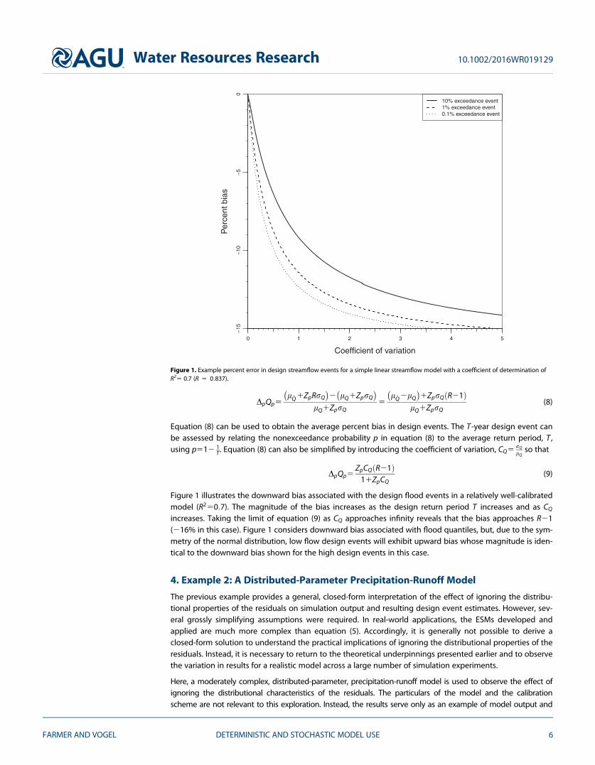
Figure 1 illustrates the downward bias associated with the design flood events in a relatively well-calibratedmodel (R250:7). The magnitude of the bias increases as the design return period T increases and as CQ

increases. Taking the limit of equation (9) as CQ approaches infinity reveals that the bias approaches R21(216% in this case). Figure 1 considers downward bias associated with flood quantiles, but, due to the sym-metry of the normal distribution, low flow design events will exhibit upward bias whose magnitude is iden-tical to the downward bias shown for the high design events in this case.

4. Example 2: A Distributed-Parameter Precipitation-Runoff Model

The previous example provides a general, closed-form interpretation of the effect of ignoring the distribu-tional properties of the residuals on simulation output and resulting design event estimates. However, sev-eral grossly simplifying assumptions were required. In real-world applications, the ESMs developed andapplied are much more complex than equation (5). Accordingly, it is generally not possible to derive aclosed-form solution to understand the practical implications of ignoring the distributional properties of theresiduals. Instead, it is necessary to return to the theoretical underpinnings presented earlier and to observethe variation in results for a realistic model across a large number of simulation experiments.

Here, a moderately complex, distributed-parameter, precipitation-runoff model is used to observe the effect ofignoring the distributional characteristics of the residuals. The particulars of the model and the calibrationscheme are not relevant to this exploration. Instead, the results serve only as an example of model output and

Coefficient of variation

Per

cent

bia

s

10% exceedance event1% exceedance event0.1% exceedance event

0 1 2 3 4 5

05

−01

−51

−

Figure 1. Example percent error in design streamflow events for a simple linear streamflow model with a coefficient of determination ofR25 0.7 (R 5 0:837).

Water Resources Research 10.1002/2016WR019129

FARMER AND VOGEL DETERMINISTIC AND STOCHASTIC MODEL USE 6

the importance of accounting for the distribution of the residuals. The distributed-parameter model, in this case,the Precipitation-Runoff Modeling System [Markstrom et al., 2008, 2015], was calibrated at each of 1225 perennialriver basins across the conterminous United States. The focus of this work is not on the development and cali-bration of this model, but rather on the impacts of its deterministic use, thus further details of the model are notprovided here. The general findings which follow are analogous to those of the previous case study and are inno way model dependent. The same general qualitative conclusions presented in the following section can beexpected to result from the use of any hydrologic model. While this is a general calibration, and other calibrationschemes may target particular extrema more directly, the theoretical argument presented remains relevant.

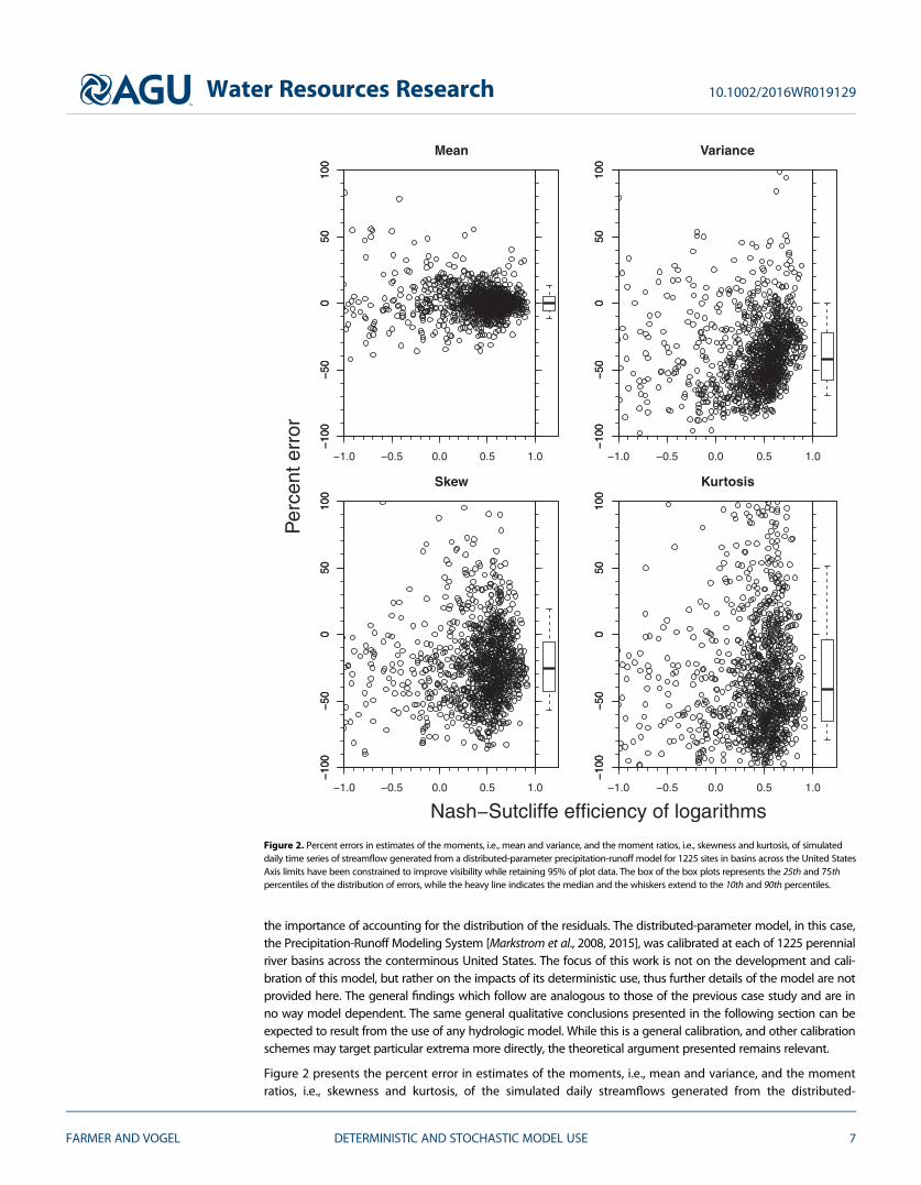
Figure 2 presents the percent error in estimates of the moments, i.e., mean and variance, and the momentratios, i.e., skewness and kurtosis, of the simulated daily streamflows generated from the distributed-

Mean

−10

0−

500

5010

0

−1.0 −0.5 0.0 0.5 1.0

−10

0−

500

5010

0

Variance

−10

0−

500

5010

0

−1.0 −0.5 0.0 0.5 1.0

−10

0−

500

5010

0

Skew

−10

0−

500

5010

0

−1.0 −0.5 0.0 0.5 1.0

−10

0−

500

5010

0

Kurtosis

−10

0−

500

5010

0

−1.0 −0.5 0.0 0.5 1.0

−10

0−

500

5010

0

Per

cent

err

or

Nash−Sutcliffe efficiency of logarithms

Figure 2. Percent errors in estimates of the moments, i.e., mean and variance, and the moment ratios, i.e., skewness and kurtosis, of simulateddaily time series of streamflow generated from a distributed-parameter precipitation-runoff model for 1225 sites in basins across the United StatesAxis limits have been constrained to improve visibility while retaining 95% of plot data. The box of the box plots represents the 25th and 75thpercentiles of the distribution of errors, while the heavy line indicates the median and the whiskers extend to the 10th and 90th percentiles.

Water Resources Research 10.1002/2016WR019129

FARMER AND VOGEL DETERMINISTIC AND STOCHASTIC MODEL USE 7

parameter precipitation-runoff models. The percent error is the error associated with using the simulatedresponse rather than the observed response. The percent errors are plotted against the Nash-Sutcliffe Effi-ciency (NSE), a metric of general performance [Nash and Sutcliffe, 1970]. NSE is essentially an estimator ofthe standardized mean square error of the simulated responses. For many reasons, the most commonlyused estimator of NSE may itself be biased and unreliable when used with daily streamflows that exhibitenormous values of skewness (see Figure 4 in Vogel and Fennessey [1993] and discussion). However, as theconcern here is more with the impact of ignoring the model residuals, NSE is included to provide a basicframe of reference. To mitigate some of the unreliability associated with the estimator of NSE that resultsfrom the underlying skewness of daily streamflow observations, the NSE was computed on the logarithmsof the daily streamflows. As expected, the models yield relatively low overall bias in the streamflows, as evi-denced by the values of percent error of the mean. The percent error in estimates of the mean, also knownas overall model bias, has a median of approximately zero (0.146%) across all sites. There is weak correlationbetween the magnitude (absolute value) of the bias and NSE, with a Spearman rank correlation of 20.327.This is not surprising, as the NSE is a measure of standardized mean square error that depends on errors inboth the mean and variance.

For the majority of sites, estimates of the variance, skewness, and kurtosis of the daily streamflows areunderestimated: the median percent errors are 241.7%, 225.2%, and 241.0%, respectively. Although thesequantities are underestimated at the majority of sites, there are several sites (less than 25% of sites) thatshow a positive bias. This is due to the fact that the covariance between the simulated response and theresiduals, discussed earlier with respect to equation (4), is seldom equal to zero and may be negative. Themagnitude of the percent error associated with the bias of these three statistics increases with decreasingmodel performance. The Spearman rank correlation between NSE and those statistics are 20.275, 20.146,and 20.116, respectively. Again, one expects NSE to be inversely related to the bias associated with anystreamflow statistic derived from the simulated model responses.

Estimates of the moment ratios, i.e., skewness and kurtosis, reported in Figure 2 are known to exhibit signifi-cant downward bias [Wallis et al., 1974], especially so for the extremely highly skewed samples of dailystreamflow considered here, even those derived from very long daily flow records [Vogel and Fennessey,1993]. Such severe downward bias, as documented by Vogel and Fennessey [1993], is inherent in all of theestimates of the moment ratios (skewness and kurtosis) reported in Figure 2 for both the observed and sim-ulated flow series. In addition, there is also downward bias in the estimated variances, which are notmoment ratios and thus not subject to the type of bias discussed by Vogel and Fennessey [1993]. Neverthe-less, to ensure that such downward bias is not due to the issues concerning the validation of stochasticstreamflow models raised by Stedinger and Taylor [1982], the same experiments in Figure 2 were performedusing equations (11)–(14) from Stedinger and Taylor [1982] with the true mean assumed equal to the histori-cal mean, as should be common practice when verifying and validating stochastic streamflow models. Theresults from those experiments led to similar results as reported in Figure 2 and thus are not reported here.

As was shown by Farmer et al. [2015] and in the previous examples, the distributional properties of theresiduals and the failure to include them in an analysis will have a strong effect on estimates of streamflowquantiles. Figure 3 shows the percent error in the estimates of various percentiles of the daily streamflowdistribution. Here, the exceedance probability is reported because that is common practice when illustratingflow duration curves. For each site, the integer percentiles from 1% to 99% were linearly interpolated fromthe observed and simulated responses. The impact of ignoring the distribution of the residuals is not asstraightforward as in the previous examples. The highest streamflows are underestimated, with a medianpercent error of 220.4% at the exceedance probability of streamflow. The low streamflows are similarlyunderestimated. For example, the streamflow exceeded only 1% of the time is underestimated with a medi-an percent error of 15.6%. There are several percentiles where the median percent error is positive. Howev-er, there are no percentiles where the direction of the bias can be uniquely categorized as positive ornegative across all sites. Though not shown, there is generally a weak negative Spearman rank correlation(a median of 20.362) between the magnitude of the percent error of streamflow quantiles and Nash-Sutcliffe efficiencies of the logarithms; the magnitude of the errors increases with decreasing model perfor-mance. Figure 3 dramatizes the complexity of the impacts of ignoring model errors when employing anESM: the resulting bias behaves in a very complex fashion across sites and across the range of streamflowexceedance probabilities of interest to hydrologists.

Water Resources Research 10.1002/2016WR019129

FARMER AND VOGEL DETERMINISTIC AND STOCHASTIC MODEL USE 8

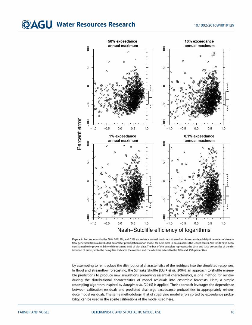
In addition to misrepresenting the distribution of the observed streamflow response, the failure to considerthe distributional properties of the residual errors can affect important decision-relevant products derivedfrom simulated ESM responses. Figure 4 demonstrates the impact of ignoring the distributional propertiesof the residual error on flood frequency analysis by focusing on the series of annual maximum streamflow(flood) events derived from the model simulations. Figure 4 reports the percent errors in estimates of designflood quantiles corresponding to exceedance probabilities of 50%, 10%, 1%, and 0.1%, which correspond toestimates of the 2, 10, 100, and 1000 year quantiles of the annual maximum daily streamflow series. Themedian percent errors are all negative, and substantially so: 230.9%, 235.7%, 239.3%, and 241.4%,respectively. Of course, none of the events are uniformly underestimated or overestimated across all sites.Certainly, as model performance degrades, the magnitude of the errors in estimates of design eventsincreases. The Spearman rank correlations between the daily model performance and the magnitude of theerrors for the four events are 20.238, 20.230, 20.229, and 20.232. Figure 4 illustrates the remarkably largeimpact of ignoring model residuals on flood frequency analysis using a general calibration of a realisticprecipitation-runoff model. The corresponding implications for water resources planning and managementare likely to be quite considerable. Studies seeking to understand why design floods estimated fromprecipitation-runoff or other deterministic models do not reproduce design floods estimated from observedstreamflow series [e.g., Di Baldassarre et al., 2010, Rogger et al., 2012, and many others] would benefit fromconsidering the issues addressed here.

5. Reintroduction of Distributional Characteristics of Residuals to ModelSimulations

The previous sections have shown the marked bias in estimates of streamflow statistics that results fromignoring the distributional properties of the residuals during model simulation. This effect can be mitigated

Exceedence probability

Per

cent

err

or

0 10 20 30 40 50 60 70 80 90 100

−10

00

100

200

300

Figure 3. Percent errors in estimated quantiles of simulated daily streamflow generated from a distributed-parameter precipitation-runoffmodel for 1225 sites in basins across the United States Axis limits have been constrained to improve visibility while retaining 95% of plotdata. The box of the box plots represents the 25th and 75th percentiles of the distribution of errors, while the heavy line indicates themedian and the whiskers extend to the 10th and 90th percentiles.

Water Resources Research 10.1002/2016WR019129

FARMER AND VOGEL DETERMINISTIC AND STOCHASTIC MODEL USE 9

by attempting to reintroduce the distributional characteristics of the residuals into the simulated responses.In flood and streamflow forecasting, the Schaake Shuffle [Clark et al., 2004], an approach to shuffle ensem-ble predictions to produce new simulations preserving essential characteristics, is one method for reintro-ducing the distributional characteristics of model residuals into ensemble forecasts. Here, a simpleresampling algorithm inspired by Bourgin et al. [2015] is applied. Their approach leverages the dependencebetween calibration residuals and predicted discharge exceedance probabilities to appropriately reintro-duce model residuals. The same methodology, that of stratifying model errors sorted by exceedance proba-bility, can be used in the at-site calibrations of the model used here.

50% exceedance annual maximum

−10

0−

500

5010

0

−1.0 −0.5 0.0 0.5 1.0

0010

001−

10% exceedance annual maximum

−10

0−

500

5010

0

−1.0 −0.5 0.0 0.5 1.0

0010

001−

1% exceedance annual maximum

−10

0−

500

5010

0

−1.0 −0.5 0.0 0.5 1.0

0010

001−

0.1% exceedance annual maximum

−10

0−

500

5010

0

−1.0 −0.5 0.0 0.5 1.0

0010

001−

Per

cent

err

or

Nash−Sutcliffe efficiency of logarithms

Figure 4. Percent errors in the 50%, 10% 1%, and 0.1% exceedance annual maximum streamflows from simulated daily time series of stream-flow generated from a distributed-parameter precipitation-runoff model for 1225 sites in basins across the United States Axis limits have beenconstrained to improve visibility while retaining 95% of plot data. The box of the box plots represents the 25th and 75th percentiles of the dis-tribution of errors, while the heavy line indicates the median and the whiskers extend to the 10th and 90th percentiles.

Water Resources Research 10.1002/2016WR019129

FARMER AND VOGEL DETERMINISTIC AND STOCHASTIC MODEL USE 10

For each site, the simulated responses were ranked and assigned a nonexceedance probability using theWeibull plotting position

pi5ri

n11

where pi is the nonexceedance probability of the i-th observation, ri is the rank of the i-th observation, andn is the number of observations. The Weibull plotting position is an attractive choice because it is known toreproduce the expected value of the unknown nonexceedance probability associated with the observa-tions, regardless of the distribution from which the observations arise [David and Nagaraja, 2003]. As inBourgin et al. [2015], model residuals were computed as the ratio of the observed response to the simulatedresponse. This practice assumes that the residuals are correlated with the simulated response and that eachresidual is simply a fraction of the original simulated response. To produce an alternate, synthetic realizationof simulated responses, the simulated daily streamflows, and their associated model residuals were groupedinto 10 equally spaced groups defined by the nonexceedance probabilities associated with each simulatedstreamflow response. For each group, the synthetic simulated response was generated by multiplying theoriginal simulated response by a random residual drawn, with replacement, from the residuals associatedwith that group. Such random resampling, with replacement, is known as the Bootstrap (e.g., see droughtexamples in Tasker and Dunne [1997] and Henley et al. [2013]). When synthetic streamflows have been gen-erated for all original simulations in all groups, the resulting series is presented in the original order and rep-resents an alternate, synthetic realization of daily streamflows with model error reintroduced. This can berepeated to produce several realizations of synthetic streamflow for the same site; a process that could leadto the generation of prediction intervals, as proposed by Bourgin et al. [2015].

The overall approach presented by Bourgin et al. [2015] and modified as described above is similar to theuse of copulas for implementing the Bootstrap. The stratification of residuals by the nonexceedance proba-bility of simulated responses is, in a loose sense, a sort of nonparametric, empirical copula. However, it isnot an exact copula, which would explicitly describe the joint distribution of a set of variables, because noeffort is made to directly reproduce the correlation between the simulated responses and the model resid-uals in the residual resampling scheme. However, because the rank of the simulated responses is used tostratify the residuals, this effectively maintains the joint distribution between the residuals and the stream-flows. Alternatively, as a parametric approach, it could have been assumed that simulated responses anderrors follow a multivariate normal distribution. However, initial evaluations not included here but based onthe assumption of multivariate normality produced synthetic series of simulated streamflows that did notmimic the observed streamflow. A different parametric copula or modified ensemble approaches [Clarket al., 2004; Schefzik et al., 2013] may be more appropriate, but our initial exploration only considers theempirical, nonparametric copula-inspired procedures described above.

Recall from Figures 2 and 3, that failing to account for the distributional properties of model residuals pro-duced substantial errors in estimates of the various moments and quantiles of the distribution of dailystreamflow. Figure 5, similar to Figure 3, illustrates the error associated with the median estimates of thevarious quantiles of the distribution of the synthetic daily streamflow series. Here the median errors arecomputed as the median of errors from 100 synthetic simulated responses produced by reintroducing mod-el residuals as described above. Comparing Figures 3 and 5, noticing the dramatic change in vertical axislimits, there is, on average, substantial reduction in the errors associated with each quantile when modelerrors are reintroduced. The median reduction in error across all sites and all quantiles is 94%. For almost allquantiles, more than 90% of the sites show smaller absolute errors than were seen when ignoring the distri-bution of residual errors. Only at the extremes do more than 10% of sites show greater percent errors whenresiduals are considered. Across all sites and all quantiles, nearly 95% of site-quantiles showed improve-ment. The median error in the first exceedance probability is now 3.15% and the median error in the 99thexceedance probability is 218.1%; in both cases, the variability in errors is greatly reduced. Though biasesremain, the improvements in the estimation of streamflow quantiles illustrated in Figure 5 have clear impli-cations for project design. These results emphasize the need for future research into more effective stochas-tic methods for the reintroduction of residuals into simulation model output.

The procedure described by Bourgin et al. [2015] and as modified above does not account for the inherentspatial or temporal correlation structure of the model residuals. Furthermore, its application is driven only

Water Resources Research 10.1002/2016WR019129

FARMER AND VOGEL DETERMINISTIC AND STOCHASTIC MODEL USE 11

by the distribution of the simulated responses. For this reason, it is unlikely to resolve the biases associatedwith centralized and standardized moments or derived products such as design quantiles of the annualmaximum or minimum series. The bias associated with moment estimates is complicated by the interactionand correlation among moments. The bias associated with design quantile estimates is largely due to theinherent temporal persistence in both the flow and residuals. Neither the interaction of moments nor tem-poral persistence are accounted for in this reintroduction method. The median percent errors of the mean,variance, skew, and kurtosis are 1.29%, 13.7%, 20.0%, and 50.8%, respectively. For the 50%, 10%, 1%, and0.1% annual maximums, the median percent errors are 22.1% 22.3%, 22.2%, and 22.7%, respectively. Exceptfor the kurtosis, these median percent errors show clear improvements over the previously reported valueswhen the median of 100 realizations, which include the reintroduction of residual errors, at each site is con-sidered. However, the improvements are highly variable and site-specific, showing that this initial methoddoes not provide reliable performance improvements for these products.

The idea of an ex post facto introduction of model residuals as an improvement to simulated modelresponses is akin to post-processing and two-stage least squares regression. In two-stage least squaresregression, an initial simulation model is developed and then a second model of the residuals or anotherindependent variable is constructed to account for information left out of the original simulation model. Avalid argument can be made that the original simulation model should just include all available informationfrom the start. The same could be argued here but requires the redevelopment of ESMs. However, regard-less of improvements in model calibration, this analysis reveals that model errors should always play a piv-otal role in environmental simulation.

It is nearly impossible for the distributions of observed and simulated responses of any deterministic modelto converge, exactly. Even with the reintroduction of model residuals, any single particular simulated seriesof responses will contain other sources of error not included in the model residuals and thus will always

Exceedence probability

Per

cent

err

or

0 10 20 30 40 50 60 70 80 90 100

−50

−40

−30

−20

−10

010

20

Figure 5. Median percent errors in estimated quantiles of daily streamflow generated from 100 synthetic realizations of a distributed-parameter precipitation-runoff model for each of 1225 sites in basins across the United States. Synthetic realizations were generated byreintroducing residual errors following the methods described herein. Axis limits have been constrained to improve visibility while retain-ing 95% of plot data. The box of the box plots represents the 25th and 75th percentiles of the distribution of errors, while the heavy lineindicates the median and the whiskers extend to the 10th and 90th percentiles.

Water Resources Research 10.1002/2016WR019129

FARMER AND VOGEL DETERMINISTIC AND STOCHASTIC MODEL USE 12

misrepresent the distribution of the observed response. There are many ways to calibrate a hydrologicmodel, but the fact remains that, even with the most targeted and evolved calibration schemes, some resid-ual error will remain in the simulated response. The tools and discussion presented here only serve to makeusers aware of the danger of the deterministic use of ESMs. With this knowledge, it is possible to makemore informed management decisions and judgments with regard to environmental systems and resour-ces. In practice, the deterministic use of environmental simulation models should be tabled in favor of atleast an ex post facto stochastic use of simulated response, whereby model residuals are reintroduced aftermodel simulation.

6. Summary and Conclusions

The deterministic use of environmental simulation models introduces substantial distributional bias intovarious important statistics computed from simulated responses. This bias is particularly severe at the distri-butional extremes corresponding to floods and droughts, regions of particular concern to hydrologists,planners, and managers. Even though a model may generate unbiased simulations overall, bias in variousimportant statistics derived from such simulations arise from ignoring the distributional properties of modelresiduals. This bias can be mitigated by considering a stochastic reintroduction of model residuals into sim-ulated responses. Exactly how to do so requires additional exploration and may depend on the particularapplication and the simulation model developed. Stochastic use, as an ex post facto solution to the problemof distributional bias, may be a more attractive approach than attempting to improve the simulation modelin question, or conducting sensitivity or uncertainty analyses. Importantly, many of the components of a rig-orous uncertainty analysis can be redirected for use in the stochastic development and implementation ofenvironmental simulation models in operational studies. Such analyses and developments may be particu-larly important within the context of the additional uncertainty corresponding to the impacts of climatechange. The findings presented here indicate that without a consideration of the stochastic component ofboth statistical and deterministic models, systematic bias will result in flood and drought applications.

These conclusions are substantiated by a theoretical analysis of the impact of model residuals and furtherevidenced by two examples presented above. The first example considered an idealized, closed-form solu-tion that demonstrates the general effects of ignoring the distribution of model residuals on the simulateddistribution of streamflow. The second example presents the case of a more complex and realisticdistributed-parameter precipitation-runoff model calibrated at each of 1225 perennial river basins acrossthe United States There, the effects of the residuals on simulated responses cannot be explicitly derived.Instead, the effects are demonstrated by an analysis of the first four moments, the distribution of stream-flow, and several design floods. The second example concludes by presenting one approach that can beused to improve the simulated response in design events. The results of this initial analysis emphasize theneed to exploit recent advances in the uncertainty analysis of environmental simulation models for the pur-pose of developing new and effective methods of reintroducing the distributional properties of residualsinto simulation output.

While this initial analysis only considered hydrologic models of streamflow time series, the general conclu-sions can be applied to almost any simulation modeling application in which extreme events play a pivotalrole. While no single solution exists, moving from the deterministic use of environmental simulation modelsto at least an ex post facto stochastic use will improve both understanding and communication of theuncertainties and biases in simulated results, which in turn should lead to improvements in the design,planning, and management of water resource systems.

ReferencesBeven, K. (2014), A framework for uncertainty analysis, in Applied Uncertainty Analysis for Flood Risk Management, edited by K. Beven and

J. Hall, Imperial College Press, London, U. K.Bourgin, F., V. Andr�eassian, C. Perrin, and L. Oudin (2015), Transferring global uncertainty estimates from gauged to ungauged catchments,

Hydrol. Earth Syst. Sci., 19(5), 2535–2546, doi:10.5194/hess-19-2535-2015.Clark, M., S. Gangopadhyay, L. Hay, B. Rajagopalan, and R. Wilby (2004), The Schaake Shuffle: A method for reconstructing space-time vari-

ability in forecasted precipitation and temperature fields, J. Hydrometeorol., 5(1), 243–262, doi:10.1175/1525-7541(2004)005<0243:TSSAMF>2.0.CO;2.

AcknowledgmentsPursuant to the U.S. GeologicalSurvey’s model and data archivepolicies, the data in support ofExample 2 will be permanentlyarchived with DOI:10.5066/F7W7TF4,which will be registered upon finalapproval and publication. Many thanksare due to Julie Kiang, GregoryMcCabe, and Lauren Hay, all of the U.S.Geological Survey, who providedcomments on early editions of thispaper. We are also indebted toNicholas C. Matalas and threeanonymous reviewers for theirconstructive and insightful commentson an earlier version of the paper.

Water Resources Research 10.1002/2016WR019129

FARMER AND VOGEL DETERMINISTIC AND STOCHASTIC MODEL USE 13

Clark, M. P., A. G. Slater, D. E. Rupp, R. A. Woods, J. A. Vrugt, H. V. Gupta, T. Wagener, and L. E. Hay (2008), Framework for understandingstructural errors (FUSE): A modular framework to diagnose differences between hydrological models, Water Resour. Res., 44, W00B02,doi:10.1029/2007WR006735.

Clark, M. P., et al. (2015a), A unified approach for process-based hydrologic modeling: 1. Modeling concept, Water Resour. Res., 51, 2498–2514, doi:10.1002/2015WR017198.

Clark, M. P., et al. (2015b), A unified approach for process-based hydrologic modeling: 2. Model implementation, Water Resour. Res., 51,2515–2542, doi:10.1002/2015WR017200.

David, H., and H. Nagaraja (2003), Order Statistics, Wiley Series in Probability and Statistics, 3rd ed., 488 pp., Wiley-Interscience, Hoboken, N. J.Di Baldassarre, G., G. Schumann, P. D. Bates, J. E. Freer, and K. J. Beven (2010), Flood-plain mapping: A critical discussion of deterministic

and probabilistic approaches, Hydrol. Sci. J., 55(3), 364–376, doi:10.1080/02626661003683389.Farmer, W. H., S. A. Archfield, T. M. Over, L. E. Hay, J. H. LaFontaine, and J. E. Kiang (2014), A comparison of methods to predict historical dai-

ly streamflow time series in the southeastern United States, Sci. Invest. Rep. 2014-5231, U.S. Geol. Surv., Reston, Va., doi:10.3133/sir20145231.

Farmer, W. H., R. R. Knight, D. A. Eash, K. J. Hutchinson, M. Linhart, D. E. Christiansen, S. A. Archfield, T. M. Over, and J. E. Kiang (2015), Evalu-ation of statistical and rainfall-runoff models for predicting historical daily streamflow time series in the Des Moines and Iowa Riverwatersheds, Sci. Invest. Rep. 2015-5089, U.S. Geol. Surv., doi:10.3133/sir20155089.

Henley, B. J., M. A. Thyer, and G. Kuczera (2013), Climate driver informed short-term drought risk evaluation, Water Resour. Res., 49, 2317–2326, doi:10.1002/wrcr.20222.

Hirsch, R. M. (1979), An evaluation of some record reconstruction techniques, Water Resour. Res., 15(6), 1781, doi:10.1029/WR015i006p01781.Hirsch, R. M. (1981), Stochastic hydrologic model for drought management, J. Water Resour. Plann. Manage., 107(WR2), 303–313.Hirsch, R. M. (1982), A comparison of four streamflow record extension techniques, Water Resour. Res., 18(4), 1081, doi:10.1029/

WR018i004p01081.Kirby, W. (1975), Model smoothing effect diminishes simulated flood peak variance, Am. Geophys. Union Trans., 56(6), 361.Lichty, R. W., and F. Liscum (1978), A rainfall-runoff modeling procedure for improving estimates of t-year (annual) floods for small drainage

basins, Water Resour. Invest. Rep. 78-7, U.S. Geol. Surv., Reston, Va.Liu, Y. Q., and H. V. Gupta (2007), Uncertainty in hydrologic modeling: Toward an integrated data assimilation framework, Water Resour.

Res., 43, W07401, doi:10.1029/2006WR005756.Markstrom, S. L., R. G. Niswonger, R. S. Regan, D. E. Prudic, and P. M. Barlow (2008), GSFLOW—Coupled ground-water and surface-water

flow model based on the integration of the Precipitation-Runoff Modeling System (PRMS) and the Modular Ground-Water Flow Model(MODFLOW-2005), Tech. and Methods 6-D1, U.S. Geol. Surv., Reston, Va.

Markstrom, S. L., R. S. Regan, L. E. Hay, R. J. Viger, R. M. T. Webb, R. A. Payn, and J. H. LaFontaine (2015), PRMS-IV, the Precipitation-RunoffModeling System, Version 4: Tech. and Methods 6-B7, U.S. Geol. Surv., Reston, Va.

Matalas, N. C., and B. Jacobs (1964), A correlation procedure for augmenting hydrologic data, Prof. Pap. 434, U.S. Geol. Surv., Reston, Va.Matott, L. S., J. E. Babendreier, and S. T. Purucker (2009), Evaluating uncertainty in integrated environmental models: A review of concepts

and tools, Water Resour. Res., 45, W06421, doi:10.1029/2008WR007301.Mirzaei, M., Y. F. Huang, A. El-Shafie, and A. Shatirah (2015), Application of the generalized likelihood uncertainty estimation (GLUE)

approach for assessing uncertainty in hydrological models: A review, Stochastic Environ. Res. Risk Assess., 29(5), 1265–1273, doi:10.1007/s00477-014-1000-6.

Montanari, A. (2011) Uncertainty of hydrological predictions, in Treatise on Water Science, edited by P. Wilderer, pp. 459–478, Elsevier,Oxford, doi:10.1016/B978-0-444-53199-5.00045-2.

Montanari, A., and D. Koutsoyiannis (2012), A blueprint for process-based modeling of uncertain hydrological systems, Water Resour. Res.,48, W09555, doi:10.1029/2011WR011412.

Moradkhani, H., and S. Sorooshian (2008), General review of rainfall-runoff modeling: Model calibration, data assimilation, and uncertaintyanalysis, in Hydrological Modeling and Water Cycle, Coupling of the Atmospheric and Hydrological Models, edited by S. Sorooshian et al.,pp. 1–24, Springer, Berlin, doi:10.1007/978-3-540-77843-1_1.

Nash, J., and J. Sutcliffe (1970), River flow forecasting through conceptual models part I—A discussion of principles, J. Hydrol., 10(3),282–290, doi:10.1016/0022-1694(70)90255-6.

Rasmussen, T. J., C. J. Lee, and A. C. Ziegler (2008), Estimation of constituent concentrations, loads, and yields in streams of Johnson Coun-ty, northeast Kansas, using continuous water-quality monitoring and regression models, October 2002 through December 2006, Sci.Invest. Rep. 2008-5014, U.S. Geol. Surv., Reston, Va.

Rogger, M., B. Kohl, H. Pirkl, A. Viglione, J. Komma, R. Kimbauer, R. Merz, and G. Bloschl (2012), Runoff model and flood frequency statisticsfor design flood estimation in Austria—Do they tell a consistent story?, J. Hydrol., 456, 30–43, doi:10.1016/j.jhydrol.2012.05.068.

Schaake, J., J. Demargne, R. Hartmen, M. Mullusky, E. Welles, L. Wu, H. Herr, X. Fan, and D. J. Seo (2007), Precipitation and temperatureensemble forecasts from single-value forecasts, Hydrol. Earth Syst. Sci. Discuss., 4, 655–717, doi:10.5194/hessd-4-655-2007.

Schefzik, R., T. L. Thorarinsdottier, and T. Gneiting (2013), Uncertainty quantification in complex simulation models using ensemble copulacoupling, Stat. Sci., 28(4), 616–640, doi:10.1214/13-STS443.

Schoups, G., and J. A. Vrugt (2010), A formal likelihood function for parameter and predictive inference of hydrologic models with correlat-ed, heteroscedastic, and non-Gaussian errors, Water Resour. Res., 46, W10531, doi:10.1029/2009WR008933.

Sherwood, J. M. (1994), Estimation of peak-frequency relations, flood hydrographs, and volume-duration-frequency relations of ungagedsmall urban streams in Ohio, Water Supp. Pap. 2432, U.S. Geol. Surv., Reston, Va.

Skøien, J. O., and G. Bl€oschl (2007), Spatiotemporal topological kriging of runoff time series, Water Resour. Res., 43, W09419, doi:10.1029/2006WR005760.

Smith, T., L. Marshall, and A. Sharma (2015), Modeling residual hydrologic errors with Bayesian inference, J. Hydrol., 528, 29–37, doi:10.1016/j.jhydrol.2015.05.051.

Stedinger, J. R., and R. M. Taylor (1982), Synthetic streamflow generation 1: Verification and validation, Water Resour. Res., 18(4), 909–918,doi:10.1029/WR018i004p00909.

Stedinger, J. R., R. M. Vogel, S. U. Lee, and R. Batchelder (2008), Appraisal of the generalized likelihood uncertainty estimation (GLUE) meth-od, Water Resour. Res., 44, W00B06, doi:10.1029/2008WR006822.

Tasker, G. D., and P. Dunne (1997), Bootstrap position analysis for forecasting low flow frequency, J. Water Resour. Plann. Manage., 123(6),359–367, doi:10.1111/j.1752-1688.1982.tb03964.x.

Thomas, W. O. (1982), An evaluation of flood frequency estimates based on rainfall/runoff modeling, J. Am. Water Resour. Assoc., 18(2),221–229, doi:10.1111/j.1752-1688.1982.tb03964.x.

Water Resources Research 10.1002/2016WR019129

FARMER AND VOGEL DETERMINISTIC AND STOCHASTIC MODEL USE 14

Vogel, R. M. (1999), Editorial: Stochastic and deterministic world views, J. Water Resour. Plann. Manage., 125(6), 311–313, doi:10.1061/(ASCE)0733-9496(1999)125:6(311).

Vogel, R. M., and N. M. Fennessey (1993), L-moment diagrams should replace product-moment diagrams, Water Resour. Res., 29(6), 1745–1752, doi:10.1029/93WR00341.

Vogel, R. M., and J. R. Stedinger (1985), Minimum variance streamflow record augmentation procedures, Water Resour. Res., 21(5), 715–723,doi:10.1029/WR021i005p00715.

Wallis, J. R., N. C. Matalas, and J. R. Slack (1974), Just a moment, Water Resour. Res., 10(2), 211–219, doi:10.1029/WR010i002p00211.

Water Resources Research 10.1002/2016WR019129

FARMER AND VOGEL DETERMINISTIC AND STOCHASTIC MODEL USE 15