![Discretization of Maxwell-Vlasov Equations based on Discrete Exterior …1276... · 2017. 9. 28. · Maxwell-Vlasov equations based on discrete exterior cal-culus [3, 5, 6] and some](https://static.fdocuments.net/doc/165x107/60e079cee64c2b05b10a79ca/discretization-of-maxwell-vlasov-equations-based-on-discrete-exterior-1276.jpg)
On the derivation of non-local diffusion equations in ... · The fractional Vlasov-Fokker-Planck...
242
On the derivation of non-local diffusion equations in confined spaces Ludovic Cesbron Supervised by Antoine Mellet and Clément Mouhot Department of Pure Mathematics and Mathematical Statistics Centre for Mathematical Sciences University of Cambridge This dissertation is submitted for the degree of Doctor of Philosophy Sidney Sussex College May 2017
Transcript of On the derivation of non-local diffusion equations in ... · The fractional Vlasov-Fokker-Planck...

On the derivation of non-local
diffusion equations in confined spaces
Ludovic Cesbron
Supervised by
Antoine Mellet and Clément Mouhot
Department of Pure Mathematics and Mathematical Statistics
Centre for Mathematical Sciences
University of Cambridge
This dissertation is submitted for the degree of
Doctor of Philosophy
Sidney Sussex College May 2017


Thesis Summary
Nonlocal diffusion equations are partial differential equations that model the frac-
tional diffusion phenomena observed, for instance, in plasma physics, and have received
a lot of attention in recent years. They involve fractional integro-differential operators,
such as the fractional Laplacian. Unlike classical derivatives, these are nonlocal in
the sense that the fractional derivative of a function at a point x will be influenced by
the behaviour of the function in the whole domain, even far away from x. The purpose
of this thesis is to understand how these nonlocal diffusion operators interact with an
external electric field or with spatial boundaries. To that end, we will adopt a kinetic
point of view on the diffusion process in order to have a more detailed understanding
of the phenomenon, and derive from kinetic equations with geometric constraints the
confined nonlocal diffusion equations.
The fractional Vlasov-Fokker-Planck equations are particularly adapted to
this purpose. Indeed, they already feature a fractional Laplacian but it acts solely on
the velocity of particles so it does not interact directly, at the kinetic scale, with the
spatial confinements we introduce. We present in this thesis a method we developed
to investigate the anomalous diffusion limit of these equations in such a way that
we can track the interaction as it arises through this limit in order to construct natural
macroscopic operators that are both non-local and adapted to the confinements we
consider.
We will first study the fractional Vlasov-Fokker-Planck equation set on the whole
space with an external electric field and show that its anomalous diffusion limit is
an advection-fractional diffusion equation if the field satisfies a precise scaling
property.
Then, we will set the kinetic equation in a bounded spatial domain and con-
sider, on the boundary of that domain, either absorption, specular reflection or
diffusive boundary conditions. We will investigate how each of these boundary con-
ditions affects the diffusion inside the domain in order to construct a new non-local
diffusion operator adapted to the boundary condition. Finally, we will estab-
lished fundamental properties of these new operators and prove the well-posedness of
the associated nonlocal diffusion equations.


À mes parents
Lydia et Louis-Marie

Statement of Originality
I hereby declare that my dissertation entitled On the derivation of non-local diffusion
equations in confined spaces is not substantially the same as any that I have submitted
for a degree or diploma or other qualification at any other University. I further state
that no part of my dissertation has already been or is concurrently submitted for any
such degree of diploma or other qualification. This dissertation is the result of my own
work and includes nothing which is the outcome of work done in collaboration except
where specifically indicated in the text.
Chapter I motivates the research problems that we address in the following chap-
ters. It gives a historical review of how our understanding of diffusion phenomena
evolved since the XIXth century, presents the mathematical framework of non-local
diffusion equations and introduces the challenges we face today with the confinement
of non-local diffusion processes. It is my own review, based on a number of references
cited throughout the chapter.
Chapter II is original research produced in collaboration with Dr. Pedro Aceves-
Sánchez. It concerns the derivation of non-local advection-diffusion equations with
an external electric field. This research problem was suggested by Prof. Christian
Schmeiser.
Chapter III is original work, it is the core of this thesis and addresses the original
question around which my Ph.D. is articulated, which is the derivation of non-local
diffusion equations in bounded domain. This research problem was suggested by Prof.
Antoine Mellet as a continuation of a previous collaboration ([CMT12]), and the work
we present was done under the supervision and with the guidance and my Ph.D. ad-
visors Prof. Antoine Mellet and Prof. Clément Mouhot.
Chapter IV is original work produced in collaboration with Dr. Harsha Hutridurga.
It concerns the application of the method presented in Chapter III to the non-fractional
case, i.e. to classical diffusion equation. The research problem arose from a discussion
between Dr. Hutridurga and myself.
Chapter V presents original and unpublished results from an on-going work in
collaboration with Prof. Antoine Mellet and Prof. Marjolaine Puel. It concerns the
derivation of non-local diffusion equations in bounded domain from kinetic equations
viii
with diffusive boundary conditions. Note that the method we develop in this appendix
is still partly formal and this work is not meant to be published individually in its
current state.
Appendix A is original work, it combines the appendices of [Ces16] and [CH16] on
which Chapter III and Chapter IV are based. It concerns the regularity of solutions
of the free transport equation in a ball with specular reflections on the boundary.
Although the results we present are tailor-made for the purposes of Chapter III and
Chapter IV, we present them separately because we feel they constitute interesting
results on their own and, moreover, because we adopted a Lagrangian approach to
this problem and consequently the proofs are rather technical and computational.
Ludovic Cesbron
May 2017

ix


Table of contents
I Introduction 1
I.1 Classical diffusion equations . . . . . . . . . . . . . . . . . . . . . . . . 5
I.1.1 The heat equation . . . . . . . . . . . . . . . . . . . . . . . . . 5
I.1.2 Microscopic description of diffusion . . . . . . . . . . . . . . . . 11
I.1.3 Kinetic equations . . . . . . . . . . . . . . . . . . . . . . . . . . 17
I.2 Non-local diffusion equations . . . . . . . . . . . . . . . . . . . . . . . . 33
I.2.1 Motivations . . . . . . . . . . . . . . . . . . . . . . . . . . . . . 33
I.2.2 Microscopic description: Lévy flights . . . . . . . . . . . . . . . 37
I.2.3 Macroscopic description: the fractional heat equation . . . . . . 41
I.2.4 Kinetic equations with heavy tailed equilibrium . . . . . . . . . 48
I.3 Confining a diffusion process . . . . . . . . . . . . . . . . . . . . . . . . 57
I.3.1 External electric field . . . . . . . . . . . . . . . . . . . . . . . . 57
I.3.2 Bounded domains . . . . . . . . . . . . . . . . . . . . . . . . . . 60
I.4 List of works presented in this thesis and perspectives . . . . . . . . . . 69
II Anomalous diffusion limit with an external electric field 79
II.1 Introduction . . . . . . . . . . . . . . . . . . . . . . . . . . . . . . . . . 79
II.1.1 The fractional Vlasov-Fokker-Planck equation . . . . . . . . . . 79
II.1.2 Preliminaries on the Fractional Fokker-Planck operator . . . . . 81
II.1.3 Main results . . . . . . . . . . . . . . . . . . . . . . . . . . . . . 83
II.2 Existence of solution . . . . . . . . . . . . . . . . . . . . . . . . . . . . 85
II.3 A priori estimates . . . . . . . . . . . . . . . . . . . . . . . . . . . . . . 90
II.4 Anomalous diffusion limit . . . . . . . . . . . . . . . . . . . . . . . . . 96
II.4.1 The non-critical case: 1/2 < s < 1 . . . . . . . . . . . . . . . . . 97
II.4.2 The critical cases s = 1/2 and s = 1 . . . . . . . . . . . . . . . . 101
IIIAnomalous diffusion limit in spatially bounded domains 103
III.1 Introduction . . . . . . . . . . . . . . . . . . . . . . . . . . . . . . . . . 104

xii Table of contents
III.1.1 Preliminaries on the fractional Fokker-Planck operator . . . . . 109
III.1.2 Main Results . . . . . . . . . . . . . . . . . . . . . . . . . . . . 111
III.2 A priori estimates . . . . . . . . . . . . . . . . . . . . . . . . . . . . . . 117
III.3 Absorption in a smooth convex domain . . . . . . . . . . . . . . . . . . 120
III.3.1 Auxiliary problem . . . . . . . . . . . . . . . . . . . . . . . . . . 121
III.3.2 Macroscopic Limit . . . . . . . . . . . . . . . . . . . . . . . . . 122
III.4 Specular Reflection in a smooth strongly convex domain . . . . . . . . 123
III.4.1 Auxiliary problem . . . . . . . . . . . . . . . . . . . . . . . . . . 124
III.4.2 Macroscopic limit . . . . . . . . . . . . . . . . . . . . . . . . . . 129
III.5 Well posedness of the specular diffusion equation . . . . . . . . . . . . 137
III.5.1 Properties and estimates of the specular diffusion operator . . . 137
III.5.2 Existence and uniqueness of a weak solution for the macroscopic
equation . . . . . . . . . . . . . . . . . . . . . . . . . . . . . . . 144
III.5.3 Identifying the macroscopic density as the unique weak solution 146
IV Classical diffusion limit in spatially bounded domains 153
IV.1 Introduction . . . . . . . . . . . . . . . . . . . . . . . . . . . . . . . . . 154
IV.1.1 The Vlasov-Fokker-Planck equation . . . . . . . . . . . . . . . . 154
IV.1.2 Main result . . . . . . . . . . . . . . . . . . . . . . . . . . . . . 156
IV.1.3 Plan of the paper . . . . . . . . . . . . . . . . . . . . . . . . . . 157
IV.2 Strategy of the proof . . . . . . . . . . . . . . . . . . . . . . . . . . . . 157
IV.2.1 Efficiency of our approach . . . . . . . . . . . . . . . . . . . . . 159
IV.3 Solutions of the Vlasov-Fokker-Planck equation . . . . . . . . . . . . . 160
IV.3.1 Existence of weak solution . . . . . . . . . . . . . . . . . . . . . 161
IV.3.2 Uniform a priori estimate . . . . . . . . . . . . . . . . . . . . . 163
IV.4 Auxiliary problem . . . . . . . . . . . . . . . . . . . . . . . . . . . . . . 165
IV.4.1 Geodesic Billiards and Specular cycles . . . . . . . . . . . . . . 166
IV.4.2 Solution to the auxiliary problem and rescaling . . . . . . . . . 168
IV.5 Derivation of the macroscopic model . . . . . . . . . . . . . . . . . . . 169
V Anomalous diffusion limit with diffusive boundary 175
V.1 Introduction . . . . . . . . . . . . . . . . . . . . . . . . . . . . . . . . . 175
V.2 Anomalous diffusion limit . . . . . . . . . . . . . . . . . . . . . . . . . 178
V.2.1 Apriori estimates . . . . . . . . . . . . . . . . . . . . . . . . . . 178
V.2.2 Auxiliary problem . . . . . . . . . . . . . . . . . . . . . . . . . . 180
V.2.3 Formal asymptotics . . . . . . . . . . . . . . . . . . . . . . . . . 183
V.3 Analysis of the non-local operator . . . . . . . . . . . . . . . . . . . . . 186
Table of contents xiii
V.3.1 Integration by parts formula . . . . . . . . . . . . . . . . . . . . 186
V.3.2 The Hilbert space Hsdiff(Ω) . . . . . . . . . . . . . . . . . . . . . 188
V.3.3 A Poincaré-type inequality for L . . . . . . . . . . . . . . . . . 191
Appendix A Free transport equation in a sphere 195
A.0.1 Explicit expression of the trajectories . . . . . . . . . . . . . . . 196
A.0.2 First and second derivatives . . . . . . . . . . . . . . . . . . . . 197
A.0.3 Fractional Laplacian along the trajectories . . . . . . . . . . . . 208
A.0.4 Change of variable . . . . . . . . . . . . . . . . . . . . . . . . . 210
A.0.5 Control of the Laplacian of η . . . . . . . . . . . . . . . . . . . 212
References 215

Chapter I
Introduction
Contents
I.1 Classical diffusion equations . . . . . . . . . . . . . . . . . . 5
I.1.1 The heat equation . . . . . . . . . . . . . . . . . . . . . . . 5
I.1.1.1 Fourier’s law and derivation of the heat equation . 5
I.1.1.2 Analysis of the heat equation in Rd . . . . . . . . 8
I.1.2 Microscopic description of diffusion . . . . . . . . . . . . . . 11
I.1.2.1 The Brownian motion . . . . . . . . . . . . . . . . 11
I.1.2.2 The Langevin equation . . . . . . . . . . . . . . . 15
I.1.3 Kinetic equations . . . . . . . . . . . . . . . . . . . . . . . . 17
I.1.3.1 Introduction to kinetic theory . . . . . . . . . . . . 17
I.1.3.2 The Fokker-Planck and Vlasov-Fokker-Planck equa-
tions . . . . . . . . . . . . . . . . . . . . . . . . . . 22
I.1.3.3 Some properties of collision operators . . . . . . . 26
I.1.3.4 Diffusion limit of kinetic equations . . . . . . . . . 28
I.2 Non-local diffusion equations . . . . . . . . . . . . . . . . . 33
I.2.1 Motivations . . . . . . . . . . . . . . . . . . . . . . . . . . . 33
I.2.2 Microscopic description: Lévy flights . . . . . . . . . . . . . 37
I.2.3 Macroscopic description: the fractional heat equation . . . . 41
I.2.4 Kinetic equations with heavy tailed equilibrium . . . . . . . 48
I.2.4.1 Anomalous diffusion limit of a Vlasov-linear relax-
ation equation . . . . . . . . . . . . . . . . . . . . 50
2 Introduction
I.2.4.2 Anomalous diffusion limit of a fractional Vlasov-
Fokker-Planck equations . . . . . . . . . . . . . . . 54
I.3 Confining a diffusion process . . . . . . . . . . . . . . . . . . 57
I.3.1 External electric field . . . . . . . . . . . . . . . . . . . . . . 57
I.3.2 Bounded domains . . . . . . . . . . . . . . . . . . . . . . . . 60
I.3.2.1 Macroscopic boundary conditions for classical dif-
fusion equations . . . . . . . . . . . . . . . . . . . 60
I.3.2.2 Kinetic boundary conditions . . . . . . . . . . . . 61
I.3.2.3 Boundary conditions for non-local diffusion equations 64
I.4 List of works presented in this thesis and perspectives . . 69
"La chaleur pénètre, comme la gravité, toutes les substances de
l’univers, ses rayons occupent toutes les parties de l’espace. Le but
de notre ouvrage est d’exposer les lois mathématiques que suit cet
élément. Cette théorie formera désormais une des branches les plus
importantes de la physique générale."
– Joseph Fourier, 1822, Théorie Analytique de la Chaleur
The term diffusion means "to spread out", it is the movement of a quantity (mass,
heat, energy...) from a region of high concentration to regions of lower concentra-
tion. Diffusion phenomena are omnipresent in our everyday life and illustrate, in a
rather explicit manner, the tendency of any natural system to evolve toward a state
of equilibrium as expressed by the second law of thermodynamics which identifies this
equilibrium as the state of maximum entropy. It is therefore not surprising that un-
derstanding the mathematical laws underlying diffusion phenomena has been one of
the most fundamental and influential problems in the history of science as predicted
by Fourier in 1822 in the quote above translated here:
Heat, like gravity, penetrates every substance of the universe, its rays
occupy all parts of space. The object of our work is to set forth the math-
ematical laws which this element obeys. The theory of heat will hereafter
form one of the most important branches of general physics.
(translation by Alexander Freeman, 1878)
3
The purpose of this introduction is to present the crucial concepts and tools that
were developed throughout history to understand and model diffusion phenomena, and
the challenges we face today to model the peculiar diffusion processes observed in plas-
mas and turbulent fluids, especially when they are confined by an external force or in
a bounded domain. The governing principle which motivates our entire presentation
is the derivation of diffusion equations from "simple" mechanisms, and especially from
models of motion for microscopic particles.
The first part of our introduction is devoted to classical diffusion equations which
model for instance the diffusion of heat through a medium or the collective motion of
particles in a rarefied gas or a fluid, near equilibrium. This is the context in which most
of the key concepts in our understanding of diffusion phenomena were introduced. We
first present Fourier’s original derivation of the heat equation via the characterisation
of the heat flux through a surface with the celebrated Fourier law. We then adopt
a microscopic point of view and introduce the Brownian motion and the Langevin
equation to model the motion of particles in a fluid and show how to recover the heat
equation from these microscopic models. This leads us naturally to the kinetic theory
of gases and the mesoscopic description of a cloud of particles. We conclude with the
diffusion limit of those kinetic equations through which we recover both the Fourier
law and the heat equation.
In the second part of this introduction we discuss the non-local nature of the trans-
port and diffusion processes observed in plasmas and turbulent fluids, and the resulting
generalisation of the concepts introduced in the classical setting. In order to derive
the kinetic and macroscopic equations that model such phenomena, we start with a
microscopic point a view and see how we can generalise the Brownian motion into
Lévy flights that fit the anomalous behaviour of particles in turbulent fluids. We then
introduce the fractional heat equation as well as fractional kinetic models, in partic-
ular the fractional Vlasov-Fokker-Planck equation, and conclude with the anomalous
diffusion limit of the kinetic equations through which we can recover non-local diffu-
sion equations, highlighting the compatibility of these descriptions.
Finally, in the third part, we confine the diffusion processes, either with a "soft"
confinement via an external electric field, or with a "hard" confinement, restricting the
process to a bounded domain. After a brief overview of the confinement of classical
diffusion models we introduce the challenges that arise when we try to confine a non-

4 Introduction
local phenomena to a bounded domain, both from a microscopic and a macroscopic
point of view, and present some of the most recent results on the subject.
The object of Chapter II, Chapter III and Chapter V of this thesis is the derivation
of non-local diffusion equations in confined spaces from kinetic equations with a strong
non-local feature. More precisely, we will mainly focus on the fractional Vlasov-Fokker-
Planck equation because it has an explicit non-local operator which acts solely on the
velocities of particles, hence it does not conflict with the spatial confinement that
we introduce. We conclude this introduction with a statement of the results we will
present in the following chapters of this thesis and the resulting perspectives.
I.1 Classical diffusion equations 5
I.1 Classical diffusion equations
We start this introduction with a rather historical – if not always chronological – pre-
sentation of how our understanding of classical diffusion evolved throughout history.
We begin with Fourier’s derivation of the heat equation via the characterisation of the
current density. Then, we explain how Brown’s observation of pollen grains suspended
in a fluid eventually led Einstein and Langevin (among others) to the mechanical ex-
planation of the diffusion process through molecular motions at the microscopic level.
This leads us to the introduction of the kinetic theory of gases and the mesoscopic
description of a cloud of particles. In particular, we show how Langevin’s approach
gives rise to the Fokker-Planck equation and we conclude this first part of the intro-
duction with the derivation of Fourier’s law and the heat equation as a limit of kinetic
equations.
I.1.1 The heat equation
I.1.1.1 Fourier’s law and derivation of the heat equation
The oldest and most fundamental diffusion equation is the heat equation which de-
scribes the diffusion of heat through a medium. It was first derived by Fourier in 1822
in his seminal work "Théorie analytique de la chaleur" [Fou22]. In the first part of
this book, he explains, based on several elaborate experiments, that:
"Pour connaître le flux actuel de la chaleur en un point p d’une droite tracée
dans un solide, dont les températures varient par l’action des molécules, il
faut diviser la différence des températures de deux points infiniment voisins
du point p par la distance de ces points. Le flux est proportionnel au quo-
tient."
In order to know the actual flux of heat at a point p on a line drawn through
a solid, whose temperatures vary under the action of molecules, one must
divide the difference in temperature of two infinitely close neighbours of
the point p by the distance between those points. The flux is proportional
to the quotient.
This law, referred to as Fourier’s law, is the first step towards the derivation of the
heat equation. This relation has been derived in several other fields of physics where
diffusion phenomena may be observed, highlighting the ubiquity of Fourier’s approach.

6 Introduction
For instance, in 1827, Ohm established in his pioneer work [Ohm27] on electrodynam-
ics a similar relation, called Ohm’s law, which reads: the current through a conductor
between two points is directly proportional to the voltage across those two points. Fur-
thermore, another remarkable analogous relation – which will be particularly relevant
in the context of this thesis – is Fick’s law, derived by Fick in 1855 in the context of
fluid dynamics in his work "On liquid diffusion" [Fic55], which states that:
"the transfer of salt and water occurring in a unit of time, between two
elements of space filled with differently concentrated solutions of the same
salt, must be, coeteris paribus, directly proportional to the difference of
concentration, and inversely proportional to the distance of the elements
from one another."
To see how we can derive the heat equation from these laws, let us consider the context
of fluid mechanics. We introduce a function ρ(t, x), called the particle density,
which describes the distribution of particles in a fluid in Rd in the sense that in an
infinitesimal volume dx centred at x, there are ρ(t, x) dx particles at time t. Then, for
any times t1 < t2 and any ball B in Rd the quantity:
∫
B
ρ(t2, x) dx−∫
B
ρ(t1, x) dx
is equal to the amount of particles that entered the ball B between times t1 and t2
minus the amount of particles that exited the ball during that same interval of time.
Fourier’s approach consists in equating this quantity with the number of particles that
went through the surface ∂B of the ball between t1 and t2. This leads naturally to
the notion of current density vector which represents the flux of particles through
a surface, similarly to the heat flux of Fourier. We define the current density J =
J(t, x) ∈ Rd by the following implicit relation: for any element of surface dS(x) centred
at x ∈ ∂B and oriented by the unit normal vector n(x):
N+ −N− = J(t, x) · n(x) dS(x) dt
where N± is the number of particles that crossed the element of surface dS(x) in the
direction ±n(x), between the time interval [t, t + dt]. Thus, we have
∫
B
(ρ(t1, x)− ρ(t2, x)
)dx = −
∫ t2
t1
∫
∂B
J(t, x) · n(x) dS(x) dt. (I.1)

I.1 Classical diffusion equations 7
Writing
ρ(t1, x)− ρ(t2, x) =
∫ t2
t1
∂tρ(t, x) dt
and
∫ t2
t1
∫
∂B
J(t, x) · n(x) dS(x) dt =∫ t2
t1
∫
B
∇x · J(t, x) dx dt
we see that
∫ t2
t1
∫
B
(∂tρ(t, x) +∇x · J(t, x)
)dx dt = 0.
Since this is true for all sets of the form [t1, t2]×B where B is a ball in Rd, this yields
the continuity equation
∂tρ(t, x) +∇x · J(t, x) = 0. (I.2)
This fundamental equation expresses the local conservation of mass, a basic property
that is naturally required for a diffusion model. However, this equation is not closed
since J is also unknown, and this is where Fourier’s law – or rather Fick’s law in this
context – comes into play. Indeed, as explained above, this law states that for any
time t and position x in the fluid, there exists D > 0 such that
J(t, x) = −D∇xρ(t, x). (I.3)
Putting together (I.2) and (I.3) we get the diffusion equation
∂tρ(t, x)−∇x ·(D∇ρ(t, x)
)= 0. (I.4)
In the context of heat diffusion, D represents the thermal conductivity of the mate-
rial and it is therefore natural, if the material is homogeneous, to assume that D is
independent of x in which case we obtain the heat equation
∂tρ(t, x)−D∆xρ(t, x) = 0. (I.5)
8 Introduction
I.1.1.2 Analysis of the heat equation in Rd
Fourier constructed solutions of the heat equation in [Fou22] through a method of
separation of variables and the development of Fourier series which allowed him to
generate solutions in terms of infinite trigonometric series. He also constructed solu-
tions in the form of integrals, developing the celebrated Fourier transform. Although
these methods are "perhaps the most powerful and most daunting aspects of Fourier’s
work" according to Narasimhan in his excellent review of the tremendous influence of
Fourier’s work [Nar99], we give here some elements of a more modern analysis of the
heat equation set on the whole space Rd which reads
∂tρ−D∆ρ = 0 (t, x) ∈ [0, T )× R
d
ρ(0, x) = ρin(x) x ∈ Rd
(I.6)
for some initial condition ρin.
I.1.1.2.1 Scaling invariance and fundamental solution
One of the most crucial characteristics of the heat equation, and the diffusion process
it models, is a particular scaling invariance which will be of importance throughout
the rest of this chapter. Consider a solution ρ of the heat equation and define, for any
a ∈ R, the rescaled function ρa:
ρa(t, x) = adρ(a2t, ax). (I.7)
Then ρa also satisfies (I.5), indeed :
∂tρa −D∆ρa = ad(a2∂tρ(a
2t, ax)−Da2∆ρ(a2t, ax))= 0.
Moreover, ρa has the same mass as ρ. Indeed we mentioned before that the continuity
equation, and henceforth the heat equation, expresses the conservation of mass for the
particle density and this constant mass is the same for ρa and ρ as can be seen easily
by an integration of the equation and simple change of variable.
The scaling invariance motivates the following construction of solutions to the heat
equation. In the one-dimensional case, if we choose a = 1/√Dt and defined a function

I.1 Classical diffusion equations 9
ρa like we did in (I.7) then we see that we can define G : R 7→ R such that
ρa(t, x) =1√Dt
ρ( 1
D,
x√Dt
)=
1√Dt
G( x√
Dt
)=
1√Dt
G(y)
where we introduced the similarity variable
y =x√Dt
.
The heat equation on ρa then reduces to a second degree ODE on G:
2G′′ + yG′ +G =(2G′ + yG
)′= 0.
As a consequence, 2G′ + yG must constant and we will assume that this constant is 0
in order to find explicitly
G(y) = Ce−y2/4
for some constant C that we determine through the conservation of mass. Assuming
ρ is of mass 1:
1 =
∫
R
ρ(t, x) dx =C√Dt
∫
R
e−x2
4Dt dx = C
∫
R
e−u2
du = 2C√π.
We have constructed the following normalised fundamental solution of the heat equa-
tion
Φ(t, x) :=1√4πDt
e−x2
4Dt .
and extending this construction to higher dimension leads to an important object in
the analysis of the heat equation:
Definition I.1.1. The fundamental solution of the heat equation (also called heat
kernel) Φ is defined on (0,+∞)× Rd as
Φ(t, x) =1
(4πDt)d2
e−|x|2
4Dt . (I.8)

10 Introduction
It is a Gaussian distribution centred around 0 with standard deviation√Dt and
it is a solution of
∂tΦ−D∆Φ = 0 (t, x) ∈ [0, T )× R
d
Φ(0, x) = δx=0 x ∈ Rd
where δ is the Dirac delta function. It allows us to construct explicit solutions to the
global Cauchy problem for the heat equation as follows:
Theorem I.1.1. If we consider ρin ∈ S ′(Rd) then the associated heat equation (I.6)
has a unique solution ρ ∈ C∞([0,+∞);S ′(Rd)) given by the convolution of the initial
datum ρin and the heat kernel Φ:
ρ(t, x) = ρin ∗ Φ(t, x) =∫
Rd
ρin(y)Φ(t, x− y) dy. (I.9)
We refer to [Tay11] for more details and the complete proof of this theorem. Note
however that the uniqueness is only asserted within the class C∞([0,+∞);S ′(Rd))
which entails bounds on the solution near infinity. If we look, instead, for solutions
in C1([0,+∞); C∞(Rd)) without any bounds on the growth at infinity, then we loose
the uniqueness as was thoroughly investigated in 1-dimension by Tychonoff [Tyc35].
However, we can recover uniqueness of solution with an explicit extra constraint. For
instance, Tychonoff showed that there is a unique solution ρ in C1([0,+∞); C∞(Rd))
whose derivatives at all orders are bounded by some M > 0:
∣∣∣∂nρ
∂xn
∣∣∣ < M.
Moreover, there is another extra condition, extremely relevant from a physical point
of view, that has received the attention P.Rosenbloom and D.Widder in [Wid44] and
[RW59] which is the non-negativity:
u(t, x) ≥ 0. (I.10)
They were able to show in 1-dimension that this condition ensures uniqueness in
C1([0,+∞); C2(Rd)), and more precisely that the unique solution of the heat equation
(I.6) that is always non-negative is precisely the one given by the convolution with the
fundamental solution (I.9). This result was generalised by D.Aronson [Aro68] [Aro71]
to higher dimensions and for a large class of parabolic PDEs.
The literature on the heat equation is quite extensive and there are many more inter-

I.1 Classical diffusion equations 11
esting results on the subject, we refer e.g. to [Eva10] or [Tay11] and references within
for more information.
I.1.2 Microscopic description of diffusion
I.1.2.1 The Brownian motion
A few years after Fourier’s derivation of the heat equation, while Ohm was applying
his approach to electrodynamics, another significant discovery was made by Scottish
botanist R. Brown [Bro28] when observing the behaviour of pollen grains suspended
in a liquid. He noticed that the grains were in a continuous motion that could not be
accounted for by currents in the fluid, which led to the first description of what is now
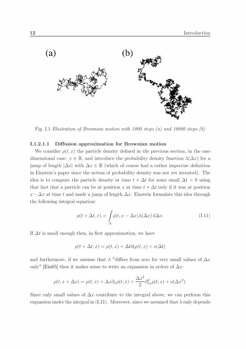
called the Brownian motion, illustrated in Figure I.1. Although the scientific com-
munity, at first, favoured the possibility that this motion was an evidence of life itself,
Brown went on to observe a similar behaviour in inorganic, hence non-living, particles
such as sand in a fluid, invalidating this possibility. The explanation for this behaviour
came with the development of Kinetic theory in the second half of the XIXth century,
which we will present in more detail in Section I.1.3. It describes the Brownian motion
as the result of an enormous amount of microscopic particles that constitute the fluid
colliding with the pollen grains which, although much bigger than the fluid particles,
are still small enough for their motion to be affected by these collisions.
When this explanation was put forward, it was far from being unequivocally accepted
by the whole scientific community, not only because the atomic theory – according to
which matter, for instance fluid, is made of a plethora of extremely small atoms and
molecules – was still the subject of controversy in the community but also because
the mathematical framework required to rigorously describe the motion observed by
Brown – for instance the notions of random walks and Markov processes – had not
yet been articulated. Indeed, those notions will only be properly defined in the early
XXth century, in particular by Pearson, Lord Rayleigh and Markov as well as Weiner
and Lévy who defined in the 1920s the Wiener processes and the Lévy processes of
which the Brownian motion is an example.
It is precisely at the beginning of the XXth century, while the formalisation of random
walks was in its beginning, that A. Einstein studied the Brownian motion from a phys-
ical point of view and was able, in 1905 [Ein05], to establish a link between Brownian
motion and diffusion processes. More precisely, he exhibited a relation between the
mean-square-displacement of Brownian particles and the diffusion coefficient of the
heat equation that governs the particle density function ρ(t, x).
12 Introduction
Fig. I.1 Illustration of Brownian motion with 1000 steps (a) and 10000 steps (b)
I.1.2.1.1 Diffusion approximation for Brownian motion
We consider ρ(t, x) the particle density defined in the previous section, in the one-
dimensional case: x ∈ R, and introduce the probability density function λ(∆x) for a
jump of length |∆x| with ∆x ∈ R (which of course had a rather imprecise definition
in Einstein’s paper since the notion of probability density was not yet invented). The
idea is to compute the particle density at time t + ∆t for some small ∆t > 0 using
that fact that a particle can be at position x at time t+∆t only if it was at position
x−∆x at time t and made a jump of length ∆x. Einstein formulate this idea through
the following integral equation:
ρ(t+∆t, x) =
∫
R
ρ(t, x−∆x)λ(∆x) d∆x. (I.11)
If ∆t is small enough then, in first approximation, we have
ρ(t+∆t, x) = ρ(t, x) + ∆t∂tρ(t, x) + o(∆t)
and furthermore, if we assume that λ "differs from zero for very small values of ∆x
only" [Ein05] then it makes sense to write an expansion in orders of ∆x:
ρ(t, x+∆x) = ρ(t, x) + ∆x∂xρ(t, x) +∆x2
2∂2xxρ(t, x) + o(∆x2).
Since only small values of ∆x contribute to the integral above, we can perform this
expansion under the integral in (I.11). Moreover, since we assumed that λ only depends
I.1 Classical diffusion equations 13
on the length |∆x| we have
〈∆x〉 :=∫
R
∆xλ(∆x) d∆x = 0
since the integrand is an odd function. Hence, if we only consider the highest order
term, (I.11) yields
∆t∂tρ(t, x) + o(∆t) =
∫
R
(∆x2
2∂2xxρ(t, x) + o(∆x2)
)λ(∆x) d∆x
so we recover in first approximation the heat equation
∂tρ(t, x) = D∂2xxρ(t, x)
where
D =1
2∆t〈∆x2〉 := 1
2∆t
∫
R
∆x2λ(∆x) d∆x.
Earlier in the same article [Ein05], Einstein computed this diffusion coefficient D by
studying the particle density ρ when the system reaches thermodynamic equilibrium.
He wrote explicitly the conditions ρ must satisfy in order for the diffusion force and
the friction force in the fluid to perfectly balance each other (dynamic equilibrium)
and, furthermore, for the energy to be constant throughout the system (thermal equi-
librium). Introducing the temperature T , the pressure P , the ideal gas constant R,
the number of particles N , the radius of the spherical particles considered r and the
viscosity of the fluid µ, he proved that the diffusion constant must be
D =RT
N
1
6πrµ.
Together, the two formulae yield the following relation between the mean-square-
displacement 〈∆x2〉 and the time step ∆t:
〈∆x2〉 = RT
N
1
3πrµ∆t. (I.12)
This formula was of particular interest to the scientific community because there was
good hope to be able to measure this mean-square-displacement and so from this

14 Introduction
relation it becomes possible to estimate not only the true size of atoms but also the
Avogadro number, i.e. the number of atoms in a mole. This was indeed eventually
obtained experimentally by Perrin in 1910 which allowed him to compute the Avogadro
number and thus consolidate the atomic theory.
Remark I.1.2. Notice how (I.12) illustrates the scaling property of the heat equation
that we presented in (I.7). If one rescales the space and time steps by some a > 0 as
∆x→ a∆x and ∆t→ a2∆t
then the relation remains unchanged.
I.1.2.1.2 The Wiener process
The formal definition of a Wiener process, the stochastic description of the Brownian
motion, reads as follows
Definition I.1.2. A Wiener process Wt is a stochastic process characterised by the
following conditions
i) W0 = 0 almost surely
ii) Wt has continuous paths, i.e. it is almost surely continuous with respect to t
iii) Wt has independent increments: for all 0 ≤ s1 ≤ t1 ≤ s2 ≤ t2, the random
variables Wt1 −Ws1 and Wt2 −Ws2 are independent.
iv) Wt has stationary Gaussian increments: for all t, s ≥ 0, Wt+s −Wt is normally
distributed with mean 0 and variance s
Wt+s −Wt ∼ N (0, s)
where N (µ, σ2) denotes the normal distribution with expected value µ and vari-
ance σ2.
The first incomplete definition of such processes was given in 1900 by Bachelier
[Bac00], a student of H. Poincaré, in the field of stock market speculations, without
any explicit mention of the Brownian motion. The rigorous proof of existence of such
processes as a limit of discrete random walks was established through several different
methods, first by Wiener in 1923 [Wie23] by introducing the Wiener measure on the
space of continuous functions on [0, 1], then by Wiener again [Wie24] using Fourier

I.1 Classical diffusion equations 15
series, then in 1931 by Kolmogoroff [Kol93] who gave a rigorous version of Bachelier’s
argument based on Gaussian martingales, and also by Lévy in 1940 [Lév80] by an
interpolation argument. The proof of Lévy is very common in modern literature on
the subject, the idea is to build a process which satisfies i), iii) and iv) on the set Dn
of dyadic numbers in [0, 1]:
Dn = k2n
: 0 ≤ k ≤ 2n
then take the limit as n goes to infinity to get a continuous process on [0, 1], extend
it to [0,+∞) and, finally, check that this extended limit, which is time-continuous by
construction, still satisfies i), iii) and iv).
I.1.2.2 The Langevin equation
The linear characterisation of the mean-square-displacement (I.12) was also derived,
three years after Einstein, by Langevin with a demonstration that was "infinitely more
simple by means of a method that is entirely different" [Lan08] to quote his own words.
Indeed, Langevin’s method differs drastically from Einstein’s because it is purely mi-
croscopic. Instead of using the Brownian motion to describe the evolution of the
particle density ρ, he uses it to describe the average motion of a particle (polen grain)
in a fluid as a result of external forces, building on the work of Smoluchowski [Smo16].
The starting point is Newton’s second law of motion applied to the position x(t) of a
particle in the fluid. Using Stokes’ formula according to which the viscosity force on
the particle is −6πµr dxdt
, this yields
md2x
dt2= −6πµr
dx
dt+X (I.13)
where µ is the viscosity of the fluid, r is the radius of the spherical particle and X is a
"complementary force that is indifferently positive and negative and its magnitude is
such that it maintains the agitation of the particle, which the viscous resistance would
stop without it".
Equation (I.13) is the first example of a wide class of stochastic differential equations
called the Langevin equation, although it is usually written for the velocity variable
v(t) = dx/ dt. In his paper, Langevin did not need to identify the process X precisely,
he only cared that its expected value E(X), or as he calls it "the average value of
the term Xx(t)", be zero which he justifies by the "irregularity of the complementary

16 Introduction
forces X" and is indeed satisfied for a Wiener process, c.f. iv) in Definition I.1.2.
Langevin multiplies the equation by x(t) to get
m
2
d2x2
dt2−m
( dx
dt
)2= −3πµr
dx2
dt+Xx (I.14)
and looks at what this equation entails when averaged over the vast number of particles
in the fluid. If the average motion x satisfies (I.14) then Langevin recognizes the
kinetic energy in the second term on the left-hand-side which is given by the thermal
equilibrium relation as:
m( dx
dt
)2=RT
2N
whereN is the number of particles, R is the ideal gas constant and T is the temperature.
Introducing the mean-square-displacement z(t) = dx2/ dt, he obtains:
m
2
dz
dt+ 3πµrz(t) =
RT
N.
He then solves this ODE for z(t) which reads, for some constant C, as
z(t) =RT
N
1
3πµr+ Ce−
6πµrm
t
and he recovers Einstein’s formula (I.12) in the "long-time" asymptotic. Note that the
coefficient in the exponential is of order 10−8 so the "long-time" is actually t greater
than 10−8 seconds.
Langevin’s work had tremendous influence over the subsequent development of kinetic
theory and stochastic calculus. Indeed, he makes the first step towards the notion of
Gaussian white noise with his force X, which he presents as a stochastic pertur-
bation of Newton’s second law of motion, hence introducing the stochastic equivalent
of Newton’s second law: the Langevin equation, making him the founder of the field
of Stochastic Differential Equations. The Langevin equation, and stochastic PDEs
in general, are now widely used to model non-deterministic phenomena, we refer to
[CKW96] for more information on the implications of Langevin’s work.

I.1 Classical diffusion equations 17
I.1.3 Kinetic equations
I.1.3.1 Introduction to kinetic theory
Kinetic theory was first developed in the second half of the XIXth century. Although
the pioneer works of Bernouilli, Clausius, Krönig and several others had a strong im-
pact on its original development, the invention of kinetic theory is accredited to L.
Boltzmann and J.C. Maxwell
Kinetic theory embodies a link between the microscopic description of a fluid (gas,
plasma, or any large cloud of particles) where we describe the movement of a single
particle using Newton’s laws of motion – or, as we have seen above, the Brownian
motion or Langevin equations – and the macroscopic description of a fluid with mod-
els such as the heat equation, the Euler equation or the Navier-Stokes equation for
example. Indeed, as we have seen in the previous sections, when we derive the heat
equation from the Brownian motion, we used a Taylor expansion and only kept the
highest order terms, loosing all the information hidden in the lower order ones. One
of the purpose of kinetic equations is then to provide us with a scale of observation
which retains all the information of the microscopic description and, at the same time,
allows us to investigate macroscopic characteristics of the fluid. The first, and most
fundamental, illustration of this idea is the Maxwell-Boltzmann distribution:
M(v) =( m
2πkT
) 32
e−mv2
2kT (I.15)
where m is a particle’s mass, T is the thermodynamic temperature and k is Boltz-
mann’s constant. It describes the distribution of the speeds of particles in idealised
gases at equilibrium and it connects the microscopic and macroscopic scales since its
variable v is inherently microscopic and it expresses how the velocities are distributed
in the whole macroscopic gas. It was heuristically derived by Maxwell in 1867 [Max67]
and Boltzmann proved in 1872 [Bol95] through his celebrated H-theorem that gases
should over time tend toward this distribution of velocities.
The key concept that led Maxwell and Boltzmann to the elaboration of kinetic theory
is the idea that all measurable quantities, i.e. all observable macroscopic characteris-
tics of a fluid, can be expressed in terms of microscopic averages. To illustrate this
idea, let us introduce the unknown of the kinetic equations we will consider: the prob-
ability density function f(t, x, v). It depends on time t ∈ [0, T ) or [0,+∞), position
x ∈ Ω ⊆ Rd and velocity v ∈ Rd. For any fixed time t, the quantity f(t, x, v) dx dv
represents the density of particles in an infinitesimal volume dx dv of the phase-space

18 Introduction
or, in other words, the density of particles in a volume dx centred at x ∈ Ω and a
velocity v′ in the neighbourhood dv of v. By the averaging of the distribution func-
tion f , we can recover macroscopic quantities such as the particle density ρ(t, x), the
macroscopic velocity u(t, x) or the local temperature T (t, x) as follows:
ρ(t, x) =
∫
Rd
f(t, x, v) dv, ρ(t, x)u(t, x) =
∫
Rd
vf(t, x, v) dv,
ρ(t, x)|u(t, x)|2 + dρ(t, x)T (t, x) =
∫
Rd
|v|2f(t, x, v) dv.(I.16)
The evolution of the distribution function f is deduced from the microscopic descrip-
tion of the motion of particles as we will present now.
I.1.3.1.1 Collisionless setting
Let us start with the simplest situation, which is the collisionless setting. We look
at a cloud of particles where the particles do not interact with each other. In first
approximation, let us assume that there is no friction, or viscosity, phenomenon. In
this setting, a particle will move in a straight line with constant velocity. The position
and velocity of a particle (x(t), v(t)) will then satisfy dxdt
= v, dvdt
= 0. If we differentiate
the distribution f along those characteristic lines we have
d
dtf(t, x(t), v(t)
)= 0
which yields the free transport equation, also called Vlasov equation:
∂tf + v · ∇xf = 0. (I.17)
Given an initial condition
f(0, x, v) = fin(x, v) (I.18)
an explicit solution is
f(t, x, v) = fin(x− tv, v).
If there is a macroscopic force E acting on the particles then their trajectories will not
be straight lines anymore. Newton’s second law of motion states that m dvdt
= E which

I.1 Classical diffusion equations 19
yields the kinetic equation (rename E := E/m):
∂tf + v · ∇xf + E · ∇vf = 0.
In particular, E could be an external electric field: E = E(t, x) independent of f , or
E could model the self-consistent electric field generated by the particles in which case
we get the celebrated Vlasov-Poisson equation
∂tf + v · ∇xf + E(t, x) · ∇vf = 0,
E(t, x) = ∇xφ(t, x), ∆xφ = ρ(t, x).
These are just two examples of macroscopic forces, one can also consider a more com-
plex self-consistent electro-magnetic field given by a coupling with Maxwell’s equations
of electromagnetic. This model is particularly relevant, for instance, when considering
quasineutral plasmas and laser-plasma interactions. It has received a lot of attention,
we refer e.g. to [GS86], [BMP03], [BGP03] or [CL06] for more information.
I.1.3.1.2 Collisional setting, the Boltzmann operator
Now, let us assume again that there are no macroscopic forces but let us consider
the collisional setting. In order to derive the kinetic equation that governs the evolu-
tion of f we need to model the collisions between particles. There are several ways
to model these collisions, we present here one of the most celebrated models: the
Boltzmann operator, and we devote Section I.1.3.2 to another remarkable model: the
Fokker-Planck operator.
The Boltzmann collision operator was first derived heuristically by Maxwell in [Max67]
and then formalised by Boltzmann in 1872 [Bol95] using the following structural as-
sumptions:
1. Binary collisions: this comes down to assuming that the gas is dilute enough to
assume that the occurrence of a collision of 3 or more particles simultaneously
is rare enough to be neglected.
2. Localised collisions: we assume collision are brief events, localised both in time
and space, meaning that the duration of collision is assumed to be very small
with respect to the time scale that we consider.
3. Elastic collisions: momentum and kinetic energy are preserved in the collision
process. This assumption yields the following relations for the collision of two
20 Introduction
particles of velocity v′ and v′∗ which acquire the velocities v and v∗ respectively
after collision: v′ + v′∗ = v + v∗
|v′|2 + |v′∗|2 = |v|2 + |v∗|2.
4. Microreversible collisions: we assume the microscopic dynamics are time-reversible
which means that the probability of a pair of velocity (v′, v′∗) to become (v, v∗)
after collision is the same as the probability of (v, v∗) to become (v′, v′∗).
5. Boltzmann’s chaos assumption: we assume that the velocities of two particles
before collision are uncorrelated. This assumption is of great importance in the
field of kinetic theory and is the subject of many works, it implies an asymmetry
between past and future which plays a crucial role in one of the most fundamental
questions of kinetic theory: the loss of reversibility when we consider a large
number of reversible dynamics.
These assumptions were stated by Boltzmann in 1872 [Bol95] and allowed him to
formally derive the Boltzmann operator to model the collisions of particles at a kinetic
scale. Note that the rigorous derivation of the Boltzmann operator from Newton’s law
of motion is still an open problem although it has been proven for very small time,
smaller than the mean time of the first collision. From the elastic collision assumption,
we deduce the σ-representation where σ ∈ Sd−1 denotes
σ =v′ − v′∗|v′ − v′∗|
with which the elastic relation can be written as
v′ =v + v∗
2+
|v − v∗|2
σ
v′∗ =v + v∗
2− |v − v∗|
2σ.
Introducing the notation f ′ = f(t, x, v′), f∗ = f(t, x, v∗) and f ′∗ = f(t, x, v′∗), the
Boltzmann operator then take the form
Q(f, f) =
∫∫
Rd×Sd−1
B(|v − v∗|, cos θ)(f ′f ′
∗ − ff∗)dv∗ dθ (I.19)
where B is the Boltzmann collision kernel and encodes the physics behind the collisions
process and cos θ is the scalar product v−v∗|v−v∗|
· σ. The kernel B can be expressed in
I.1 Classical diffusion equations 21
several different ways and we refer e.g. to [Cer88], [FS02] and references within for
detailed examples. What remains invariant, whatever the kernel we consider, is that
the Boltzmann operator can formally be expressed as a difference of two terms:
Gain and Loss
Q(f, f)(t, x, v) = Q+(f, f)(t, x, v)−Q−(f, f)(t, x, v)
where the gain term Q+ represents the number of particles that had a velocity v′
and acquired the velocity v as a result of collisions and the loss term Q− represents
the number of particles that had velocity v and lost it, to acquire another velocity
v′ after collisions. Note however that in many cases both Q+ and Q− are infinite
when written separately, which is why this formulation is formal. Nevertheless, it
motivates a simpler version of this collision operator: the linear Boltzmann operator,
which preserves this structure of gain and loss but through a linear interaction instead
of the bilinear operator written above. Considering a non-negative collision kernel
σ = σ(v, v′), the linear Boltzmann operator LB reads
LB(f) =
∫
Rd
(σ(v, v′)f ′ − σ(v′, v)f
)dv′ (I.20)
where σ(v, v′) represents the probability for a particle with velocity v to acquire the
velocity v′ after collisions. Note that this operator is not to be confused with the
linearised Boltzmann operator, which is the linearisation of Q(f, f) around its equilib-
rium.
In this thesis, our focus does not lie in the study of the linear Boltzmann operator but
we will present a few results on a particularly simple version of this operator because of
their significant influence. This simple case is sometimes called the linear relaxation
operator and corresponds to the linear Boltzmann with σ(v, v′) =M(v) where M is
the local Maxwellian
M(v) =1
(2π)d/2e−
|v|2
2 (I.21)
which yields
L(v) = ρ(t, x)M(v)− f(t, x, v). (I.22)
Although quite simplistic, this operator conserves the relaxation property of the Boltz-
mann equation which is crucial in our analysis, as we will see in section I.1.3.4. The

22 Introduction
kinetic equation associated with this operator takes the form of a balance between the
free-transport and collision. It reads
∂tf + v · ∇xf = ρ(t, x)M(v) − f(t, x, v) (I.23)
and is often called the Vlasov-linear relaxation equation.
I.1.3.2 The Fokker-Planck and Vlasov-Fokker-Planck equations
The Fokker-Planck equation was first derived by Fokker in 1914 [Fok14] and Planck
in 1917 [Pla17] to describe the evolution of the velocities of particles in a fluid. It was
independently discovered by Kolmogoroff in 1931 [Kol93] through a significantly dif-
ferent method, which is why it is sometimes referred to as the Kolmogoroff forward
equation, and it was applied by Smoluchowski [Smo16] to particle diffusion in which
case it is called the Smoluchowski equation.
The Fokker-Planck equation expresses a balance between a drift and a diffusion force,
much like the Langevin equation dissociates Stokes’ viscosity from the Brownian mo-
tion. We will show how it can be derived by a generalisation of Einstein’s diffusion
approximation. Note that we do not follow the original derivation of Fokker and
Planck but, instead, one based on the works of Kramers [Kra40], Moyal [Moy49] and
Pawula [Paw67].
I.1.3.2.1 Derivation of the Fokker-Planck equation
We consider a velocity probability density W (t, v) – equivalent of the particle density
ρ(t, x) but for the velocities – which describes the velocity distribution in a fluid. In
order to generalise Einstein’s approach, we define a conditional transition probability
λ(t+∆t, v|t, v′) that a particle with velocity v′ at time t acquires a velocity v at time
t +∆t. The integral relation (I.11) then reads
W (t+∆t, v) =
∫
Rd
W (t, v −∆v)λ(t+∆t, v|t, v −∆v) d∆v. (I.24)
Remark I.1.3. Note that the most general form of this equation would be to consider
that λ depends on the velocities at all the previous times t − k∆t, 0 ≤ k ≤ t/∆t. We
implicitly assumed here that λ has no memory in the sense that it only depends on
the velocity at times t. This is equivalent to assuming that a process with transition
probability λ satisfies the Markovian property. We refer to [Ris96, Section I.2.4.1] for
more details.

I.1 Classical diffusion equations 23
We introduce the notation Mn(v −∆v, t,∆t), n ≥ 0 for the moments of the tran-
sition probability as a function ∆v defined as
Mn(t,∆t, v) =
∫
Rd
(∆v)nλ(t+∆t, v +∆v|t, v) d∆v. (I.25)
Assuming we know those moments, we can write the Taylor expansion of the integrand
in (I.24) as
W (t, v −∆v)λ(t+∆t, v|t, v −∆v) = W (t, v −∆v)λ(t+∆t, v −∆v +∆v|t, v −∆v)
=∞∑
n=0
(−1)n
n!(∆v)n
dn
dvn
[W (t, v)λ(t+∆t, v +∆v|t, v)
]
and integrating with respect to ∆v (assuming the necessary convergence of the series
and the moments) this yields using (I.24) on the left-hand-side, and (I.25) on the
right-hand-side
W (t+∆t, v) =∞∑
n=0
(− d
dv
)n[Mn(t,∆t, v)
n!W (t, v)
].
Now, we first notice that since λ is a probability density, M0(t,∆t, v) =∫λ d∆v = 1.
For the moments Mn, n ≥ 1 we want to do a first order Taylor expansion with respect
to time, assuming ∆t is small. Since we have obviously
λ(t, v|t, v′) = δv=v′
for all v, v′, the order 0 term in the Taylor expansion will be null for all Mn. Hence,
we define the expansion coefficients mn(t, v) by the implicit relation
Mn(t,∆t, v)
n!= mn(t, v)∆t +O(∆t2).
Putting the n = 0 term on the left-hand-side and dividing by ∆t this yields
W (t+∆t, v)−W (t, v)
∆t=
∞∑
n=1
(− d
dv
)n[mn(t, v)W (t, v)
]+O(∆t).
24 Introduction
Finally, taking the limit as ∆t goes to 0 we get the Kramers-Moyal equation for
W (t, v):
∂tW (t, v) =
∞∑
n=1
(− d
dv
)n[mn(t, v)W (t, v)
].
Remark I.1.4. It goes without saying that the derivation of the Kramers-Moyal equa-
tion that we just presented is quite formal and one would need to control the conver-
gence of the sums and integrals in order to make it rigorous but that is not our purpose
here. We refer to [Ris96, Chapter 4] for more details on this derivation, as well as the
original papers of Kramers [Kra40] and Moyal [Moy49].
In 1967, in an effort to justify the Fokker-Planck model, Pawula proved in [Paw67]
by a subtle use of the generalised Cauchy-Schwarz inequality on the family of moments
Mn, that given the assumption we made on λ, there are only three possibilities:
• All moments of order n > 1 are null
• All moments of order n > 2 are null
• An infinite number of moments are not null
Pawula was able to make an explicit link between those three situations and the
underlying process described by the transition probability λ. Indeed, he proved that
if the process is deterministic, i.e. no randomness: the particle moves right at every
time step ∆t with speed m1(t, v), then we are in the first situation with a hyperbolic
transport equation: ∂tW (t, v) = −∇v
[m1(t, v)W (t, v)
]
W (0, v) = Win(v)
the solution of which if m1 = c constant is W (t, v) = Win(v − ct). Furthermore, if
the underlying process is governed by a Langevin equation then we are in the second
case and the moments m1 and m2 represent the viscosity and the diffusion coeffi-
cients −µ(t, v) and D(t, v) respectively and we obtain the general Fokker-Planck
equation
∂tW =d
dv
[µvW
]+
d2
dv2[DW
]. (I.26)
I.1 Classical diffusion equations 25
In this thesis we will focus on the case where the viscosity and diffusion coefficients µ
and D are constant in which case the Fokker-Planck equation reads
∂tW = µ∇v ·(vW)+D∆W. (I.27)
Remark I.1.5. The third case of Pawula’s theorem may be useful in some cases, for
instance to model Generation and Recombination processes, see e.g. [Ris96, Section
I.4.5], but in those cases the transition probability must be allowed to take negative
values, at least for small times, which is not very relevant when modelling fluids.
I.1.3.2.2 Solutions of the Fokker-Planck equation in Rd
Like the heat equation, the Fokker-Planck equation (I.27) is a linear parabolic PDE
and admits a Green function i.e. a fundamental solution ΦFP defined on (0,+∞)×Rd
as
ΦFP (t, x) =
(µ
2πD(1− e2µt)
) d2
e− µ|x|2
2D(1−e−2µt) (I.28)
which is solution of the Fokker-Planck equation with localised initial datum
∂tΦFP = µ∇v · (vΦFP ) +D∆vΦFP = 0 (t, v) ∈ [0, T )× R
d
ΦFP (0, v) = δv=0 v ∈ Rd.
Analogously to the fundamental solution for the heat equation, ΦFP allows us to con-
struct global solutions for the Fokker-Planck equation with initial condition W (0, v) =
Win(v) ∈ S ′(Rd) by a convolution in v
W (t, v) = Win ∗ ΦFP (t, v).
I.1.3.2.3 Derivation of the Vlasov-Fokker-Planck equation
Fokker and Planck’s approach can be extrapolated to define a collision operator at
the kinetic scale, which will actually be the main focus of all the results we present
in this thesis. The derivation of the kinetic Fokker-Planck equation differs from the
derivation of the kinetic Boltzmann equation in the same way that Langevin’s proof
of the linearity of the mean-square-displacement differs from Einstein’s. Instead of a
gain-loss approach, we take a microscopic point of view and describe the position and
velocity of a particle in the fluid by the random variables (x(t), v(t)) whose evolution
26 Introduction
is governed by a free-transport/Langevin equation:
x = v(t)
v = −µv(t) +DBt
(I.29)
where Bt is a Wiener process and the dot denotes the derivative in time. The first
equation describes the free-transport of particles as presented earlier in the collisionless
setting, and the second describes the evolution of the velocity as a balance between
a friction force and a Brownian motion. The associated kinetic equation is called the
Vlasov-Fokker-Planck equation, it reads
∂tf + v · ∇xf = µ∇v ·(vf)+D∆vf (I.30)
and we will systematically assume µ = D = 1 without loss of generality for the math-
ematical analysis of the equation. This equation is also sometimes called the Kramers
equation in reference to Kramers’ work including the derivation of the Kramers-Moyal
equation, or also the Smoluchowski equation in the 1-dimensional case.
I.1.3.3 Some properties of collision operators
In the rest of this section, we will focus on the linear relaxation and the Fokker-Planck
operator, right-hand-side of (I.23) and (I.30) respectively. Before we derive the heat
equation from the associated kinetic models, which is the subject of the following
section, we would like to present some fundamental properties that these operators
have in common. The first and most obvious property is the conservation of mass
which follows from∫
Rd
L(f) dv = 0
where L is either the linear relaxation or the Fokker-Planck operator. Note that
this property follows directly from the definitions of our operators. Another crucial
property is the existence and uniqueness of an equilibrium:
Proposition I.1.6. Let L be either the linear relaxation (I.22) or the Fokker-Planck
(I.27) operator, then there exists a unique normalised equilibrium M :
∃!M(v) ≥ 0 on Rd,
∫
Rd
M(v) dv = 1, L(M) = 0
I.1 Classical diffusion equations 27
and this equilibrium is a local Maxwellian distribution
M(v) =1
(2π)d/2e−|v|2/2. (I.31)
This should be interpreted in the light of Boltzmann’s H-theorem as an illustration
of the compatibility of our models of collision and the Maxwell-Boltzmann equilibrium
distribution of velocities. The third property which we will be central to the diffusion
limit and is common to both operator, is their dissipativity:
Proposition I.1.7. For any f(x, v) regular enough, the dissipation D, defined as
D(f) := −∫∫
Rd×Rd
fL(f)dx dv
M(v)
where M is the equilibrium (I.31), satisfies
D(f) ≥ C
∫∫
Rd×Rd
(f − 〈f〉M
)2 dx dvM(v)
≥ 0 (I.32)
for some constant C independent of f , with 〈f〉 =∫f dv.
This is a crucial property of collision operators that is very useful for the physical
justification of a kinetic equation. Indeed, we see in (I.32) that the dissipation controls
the distance between the probability density f and the velocity-equilibrium state of the
cloud of particle where the velocities are distributed according to the local Maxwellian
(I.21). As a consequence, proving that the dissipation decreases towards 0 entails the
convergence of the system towards a velocity-equilibrium state, in accordance with the
second law of thermodynamics.
Note that in the Fokker-Planck case, the dissipation takes the form of a homogeneous
H1 norm in a weighted space:
DFP (f) =
∫∫
Rd×Rd
∣∣∣∇v
( fM
)∣∣∣2
M dx dv
and since the weight is a local Maxwellian, we can use the Poincaré inequality to show
(I.32). In the linear-relaxation case, on the other hand, (I.32) is actually an equality
and the proof does not involve the gradient.
The Cauchy problem for kinetic equations with either a linear Boltzmann operator,
including the linear-relaxation case (I.23), or a Fokker-Planck operator (I.30) with
28 Introduction
or without a Poisson potential have received a great deal of interest throughout the
years. We refer e.g. to the excellent books [Cer88] and [FS02] and references within for
the Boltzmann case, and to [Bou93] and [CS95] for the Vlasov-Poisson-Fokker-Planck
(VPFP) equation, as well as [VO90] where the authors construct global solutions by
generalising a fundamental solution argument for the VPFP system. In the context of
this thesis, the existence result that is the most relevant (although far from optimal)
is the following.
Theorem I.1.8. Consider an initial condition fin such that
fin ≥ 0
fin ∈ L2M−1(Rd × R
d) where M(v) is the equilibrium (I.31)
Then the Cauchy problem
∂tf + v · ∇xf = L(f) (t, x, v) ∈ [0,+∞)× R
d × Rd
f(0, x, v) = fin(x, v) (x, v) ∈ Rd × R
d(I.33)
where L is either a linear relaxation operator (I.22) or a Fokker-Planck operator (I.27),
admits a weak solution f ∈ C0([0,+∞), L1(Rd × Rd)) which satisfies
f ≥ 0
f(t, ·, ·) ∈ L2M−1(Rd × R
d)
Note in particular that this notion of weak solution is physically relevant in the
sense that it entails finite mass, kinetic energy and entropy.
I.1.3.4 Diffusion limit of kinetic equations
Since we know that the particle density ρ can be obtained by averaging the kinetic
solution f of (I.33), as expressed in (I.16), it is only natural to wonder if we can
derive the equations that govern ρ from kinetic equations. This is the subject of this
section. For the Vlasov-Fokker-Planck equation, the answer to this question began
with the pioneer works [Wig61], [LK74] and [HM75], was rigorously established in one-
dimension in [DMG87], extended to two and three dimensions for small time interval
in [PS00], long time interval in [Gou05] and to higher dimension in [EGM10].
The first thing we notice is that the unit of time and space that we implicitly used when
deriving the Langevin equation, which we used again to derive the kinetic equation,
is much smaller than the time and space scales that are naturally used for the heat
I.1 Classical diffusion equations 29
equation. Indeed, the unit of time in the kinetic equation is linked to the time scale of
the collision process which is of the order of the average time between two consecutive
collisions of a particle, whereas in the macroscopic heat equation, a vast number of
collisions happen per unit of time. Same goes for the unit of distance which, at the
kinetic scale, is comparable to the mean-free-path: the average distance a particle
travels between two collisions, whereas at the the macroscopic scale there are about
1023 particles in a "small" element of volume so the macroscopic unit of distance is
much greater than the mean-free-path. Hence, to derive macroscopic equations from
the kinetic ones we need to rescale time and space, and to that end we introduce
the Knudsen number ε, named after Danish physicist Knudsen from the late XIXth
early XXth century, formally defined as the ratio
ε =mean-free-path
considered length scale. (I.34)
The Knudsen number formalises a continuum between the kinetic scale at ε = 1 and
the macroscopic scale in the limit as ε goes to 0. We rescale the space variable x as
x′ = εx (I.35)
and since our purpose is to derive a diffusion equation for ρ we will choose the rescaling
of time that agrees with the time linearity of the mean-square-displacement (I.12),
hence:
t′ = ε2t. (I.36)
This is called a parabolic scaling. Investigating the asymptotic behaviour, as ε goes to
0, of the resulting rescale kinetic equation and its rescaled solution fε, is usually called
taking the diffusion limit of the kinetic equation. Other rescaling limits can be
considered, such as the hyperbolic or hydrodynamical limit which allows e.g. to derive
the Euler or the Navier-Stokes equations from the Boltzmann equation, and we refer
to [MSR03], [JLM09] and references therein for more information on that topic.
With the parabolic scaling, the rescaled kinetic equations become
ε2∂tfε + εv · ∇xfε = L(fε) (t, x, v) ∈ [0,+∞)× R
d × Rd
fε(0, x, v) = fin(x, v) (x, v) ∈ Rd × R
d.(I.37)

30 Introduction
We split the study of the behaviour of fε as ε goes to 0 in two steps. First, we establish
a priori estimates in order to prove existence of a limit for the sequence fε and then
we identify that limit.
I.1.3.4.1 A priori estimates
We are interested in a priori estimates that express the tendency of the system to
tend towards its velocity equilibrium. The particular choice of scaling (I.35)-(I.36)
actually ensures that in the limit as ε goes to 0 we will have reached the velocity-
equilibrium state but not the equilibrium with respect to the position variable. This
is the whole purpose of our analysis: determine the evolution of the particle density ρ
at a scale where the velocities of the particle can be assumed to be distributed by a
local Maxwellian.
From the dissipativity of the operator, the linearity of the kinetic equations and the
regularity of the solution stated in Theorem (I.1.8), we can derive the following bounds
on the density ρε defined as
ρε(t, x) =
∫
Rd
fε(t, x, v) dv
and the energy functional Eε, sum of kinetic energy and log-entropy:
Eε(t) =∫∫
Rd×Rd
( |v|22
+ ln fε
)fε dx dv.
Theorem I.1.9. Let fε be a solution of of (I.37) in the sense of Theorem I.1.8, then
we have
i) fε is bounded in L∞([0,+∞), L2M−1(Rd × Rd)) uniformly in ε
ii) ρε is bounded in L∞([0,+∞), L2(Rd)) uniformly in ε
ii) ‖fε − ρεM‖L2M−1 (R
d×Rd)= O(ε)
iv) Eε is bounded in L∞([0,+∞)) uniformly in ε.
These uniform controls yield the existence of a limit of fε in the following sense
Proposition I.1.10. fε converges weak-∗ in L∞([0,+∞), L2M−1(Rd × R
d)) towards
ρ(t, x)M(v) where ρ is the weak limit of ρε.

I.1 Classical diffusion equations 31
I.1.3.4.2 Identifying the limit
In order to identify the limit, the idea of Poupaud and J.Soler in [PS00] was to follow
Fourier’s argument from a kinetic stand-point. They integrate the kinetic equation to
recover a kinetic version of the continuity equation (I.2):
∂tρε +1
ε∇x · jε = 0 (I.38)
where jε is the kinetic equivalent of the current density vector, defined as
jε(t, x) =
∫
Rd
vfε(t, x, v) dv.
From Fourier’s law, we expect jε to be related to the gradient of ρε, at least in the
limit as ε goes to 0. Multiplying (I.37) by v, integrating and dividing by ε, they find
an equation satisfied by jε (at least in the sense of distributions)
ε∂tjε +∇x ·∫
Rd
v ⊗ vfε dv = −CLεjε.
where CL is either 1 or d depending on the operator we consider. Moreover, they
introduce a function hε defined as
hε(t, x, v) =1
ε
(2∇v
(√f)+ v√f)
with which the second term on the left-hand-side can be expressed as
∫
Rd
v ⊗ vfε dv = ε
∫
Rd
hε ⊗ v√fε dv + ρεId.
Note that hε satisfies
∫∫
Rd×Rd
|hε|2 dx dv =d
dtEε(t).
Since the functional Eε will be constant when the system reaches its velocity-equilibrium
state, i.e. when ε goes to 0, we get
∫
Rd
v ⊗ vfε dv → ρId.

32 Introduction
and as a consequence
CLεjε → −d∇xρ
which is exactly Fourier’s law. In other words, we have just justified Fourier’s law
from a kinetic point of view by expressing how, when the system reaches its velocity
equilibrium, the flux of particles through a unit of surface, jε, converges towards the
gradient of temperature. Moreover, we see that the error between the kinetic flux
and the gradient of temperature can be measured by the kinetic energy and entropy
functional Eε.Finally, taking the limit in the continuity equation yields the diffusion limit:
Theorem I.1.11. The limit ρ(t, x) of ρε satisfies the heat equation
∂tρ = ∆ρ (t, x) ∈ [0,+∞)× Rd
ρ(0, x) = ρin(x) =
∫
Rd
fin(x, v) dv x ∈ Rd.
I.2 Non-local diffusion equations 33
I.2 Non-local diffusion equations
As we have seen in the previous section, one of the central results of Einstein’s theory –
as well as the Maxwell’s and Boltzmann’s work on kinetic theory and also the works of
Langevin, Fokker, Planck etc – is that the mean-square-displacement of the particles
scales linearly with time:
〈∆x2〉 ∼ D∆t.
Despite the omnipresence of classical diffusion, which we characterise by this linearity,
it is not universal. In fact, many experimental measurements have exhibited mean-
square-displacements that scale as a fractional power law with time:
〈∆x2〉 ∼ D∆tα (I.39)
with α > 0. This non-linearity changes drastically the diffusion phenomena and we
present in this section the associated models at the microscopic, the macroscopic and
the kinetic scale.
We start with a brief review of some physical experiments that illustrate non-linear
mean-square-displacements. Then, we introduce the mathematical tools used to model
such non-classical diffusion phenomena, both at a microscopic scale with a generalisa-
tion of Brownian motion and at a macroscopic scale with non-local diffusion operators
and the associated fractional functional spaces. Finally, we introduce kinetic equa-
tions associated with the anomalous diffusion phenomena and show how we can derive
macroscopic non-local diffusion equations from these kinetic models set in the whole
space Rd, generalising the results we have obtained in the classical case.
I.2.1 Motivations
We begin with the experiment of rotating annulus presented by T. Solomon, E. Weeks
and H. Swinney [SWS94] in 1994 and E. Weeks, J. Urbach and H. Swinney in 1996
[WUS96]. This experiment consists in a fast rotating annulus filled with fluid that
is being pumped in and out of the annulus through holes in the bottom in order to
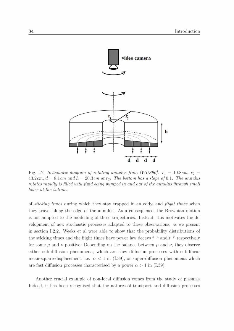
generate a turbulent flow, as illustrated in Figure I.2.
A camera on top of the annulus records the formation of turbulent eddies (small
whirlpools) inside the annulus and allows the tracking of tracer particles injected
into the fluid and the drawing of their orbits, as shown in Figure I.3. Looking at
these orbits, we see that the trajectories of tracer particles consist of the succession
34 Introduction
Fig. I.2 Schematic diagram of rotating annulus from [WUS96]. r1 = 10.8cm, r2 =43.2cm, d = 8.1cm and h = 20.3cm at r2. The bottom has a slope of 0.1. The annulusrotates rapidly is filled with fluid being pumped in and out of the annulus through smallholes at the bottom.
of sticking times during which they stay trapped in an eddy, and flight times when
they travel along the edge of the annulus. As a consequence, the Brownian motion
is not adapted to the modelling of these trajectories. Instead, this motivates the de-
velopment of new stochastic processes adapted to these observations, as we present
in section I.2.2. Weeks et al were able to show that the probability distributions of
the sticking times and the flight times have power law decays t−µ and t−ν respectively
for some µ and ν positive. Depending on the balance between µ and ν, they observe
either sub-diffusion phenomena, which are slow diffusion processes with sub-linear
mean-square-displacement, i.e. α < 1 in (I.39), or super-diffusion phenomena which
are fast diffusion processes characterised by a power α > 1 in (I.39).
Another crucial example of non-local diffusion comes from the study of plasmas.
Indeed, it has been recognised that the natures of transport and diffusion processes
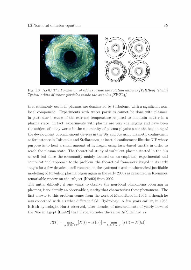
I.2 Non-local diffusion equations 35
Fig. I.3 (Left) The Formation of eddies inside the rotating annulus [VIKH08] (Right)Typical orbits of tracer particles inside the annulus [SWS94].
that commonly occur in plasmas are dominated by turbulence with a significant non-
local component. Experiments with tracer particles cannot be done with plasmas,
in particular because of the extreme temperature required to maintain matter in a
plasma state. In fact, experiments with plasma are very challenging and have been
the subject of many works in the community of plasma physics since the beginning of
the development of confinement devices in the 50s and 60s using magnetic confinement
as for instance in Tokamaks and Stellarators, or inertial confinement like the NIF whose
purpose is to heat a small amount of hydrogen using laser-based inertia in order to
reach the plasma state. The theoretical study of turbulent plasma started in the 50s
as well but since the community mainly focused on an empirical, experimental and
computational approach to the problem, the theoretical framework stayed in its early
stages for a few decades, until research on the systematic and mathematical justifiable
modelling of turbulent plasma began again in the early 2000s as presented in Krommes’
remarkable review on the subject [Kro02] from 2002.
The initial difficulty if one wants to observe the non-local phenomena occurring in
plasmas, is to identify an observable quantity that characterises these phenomena. The
first answer to this problem comes from the work of Mandelbrot in 1965, although he
was concerned with a rather different field: Hydrology. A few years earlier, in 1956,
British hydrologist Hurst observed, after decades of measurements of yearly flows of
the Nile in Egypt [Hur52] that if you consider the range R(t) defined as
R(T ) = maxt0≤t≤t0+T
[X(t)−X(t0)
]− min
t0≤t≤t0+T
[X(t)−X(t0)
]
36 Introduction
where X(t) is the river’s level, and the standard deviation S given by
S =√
〈[X ]2〉 − 〈[X ]〉2
where 〈·〉 is the mean value, then the mean value of the ratio R(T )/S grows as a power
law:⟨R(T )
S
⟩= CTH
for some constant H which, according to Hurst’s computation, is around 3/4. Fur-
thermore, Hurst goes on in [Hur56] to show that the same power-law growth can be
observed for the river’s discharges and runoffs, as well rainfalls, temperatures, pres-
sures and annual growths of tree rings, always with a constant H which varies between
1/2 and 1 and is usually around 3/4. In his seminal work [Man65], Mandelbrot es-
tablished a relation between Hurst’s exponent H and the self-similar property of the
Brownian motion. More precisely, Mandelbrot explains that if we consider the years
to be independent of each other and X(t) to be a Wiener process, then, as was proven
by Feller in 1951 [Fel51] we have
⟨R(T )
S
⟩= CT 1/2
which is a consequence of the self-similar property of the Brownian motion, i.e. if
X(t), t ∈ R is a Wiener process then for all a > 0
X(at), t ∈ R d= a1/2X(t), t ∈ R
whered= means the two process have the same finite-dimensional distributions. This
fundamental property of the Brownian motion, which results from its link with the
Normal distribution and expresses at the microscopic scale the scaling invariance of
the heat equation (I.7), can be recovered, for instance, through the autocovariance
identity of the Brownian motion: E[X(t1)X(t2)] = min(t1, t2) which yields
E[X(at1)X(at2)
]= min(at1, at2) = amin(t1, t2) = E
[(a1/2X(t1)
)(a1/2X(t2)
)].
Mandelbrot arrives to the conclusion that, although the Brownian motion cannot be
used to model the quantity Hurst studied, we should be able to describe them by a
generalisation of the motion into a stochastic process X(t), t ∈ R with mean value
I.2 Non-local diffusion equations 37
zero and such that for some constant H > 0:
X(at), t ∈ R d= aHX(t), t ∈ R. (I.40)
We will present in the next section two of the most celebrated generalisations of the
Wiener process that satisfy this same self-similar property: the fractional Brownian
motion and the Lévy flights. These generalisations are widely use in the microscopic
description of non-local diffusion processes and, moreover, the Hurst exponent H an-
swers the question we asked above: it is a measurable quantity that characterises the
non-local nature of transport and diffusion in plasmas. There have been many ex-
periments concerned with determining Hurst’s exponent, often focusing on the edge
fluctuation of plasma under magnetic confinement, and we refer the reader e.g. to
[CHS+96] [CVMP+98] or the review paper [Car97] as well as [WSL+01], [NGNR04],
[SGL+04] and [SVV04] and references within for further experimental results.
Non-local phenomena arise in many other fields and although we will not present
all of them for obvious reasons, here are some references for the interested reader:
• Sub-diffusive phenomena: charge carrier transport in amorphous semiconduc-
tors [GSG+96], nuclear magnetic resonance diffusometry in percolative [KMK97]
and porous systems [Kim97], rouse or reptation dynamics in polymetric systems
[FKB+99], transport on fractal geometries [HMTW85] [PBHR97], the diffusion
of a scalar tracer in an array of convection rolls [YPP89], the dynamics of a bead
in a polymetric network [AMY+96] [BS99].
• Super-diffusive phenomena: collective slip diffusion on solid surfaces [LL99], lay-
ered velocity fields [MDM80] [ZKB91], Richardson turbulent diffusion [Ric26]
[SWK87], bulk-surface exchange controlled dynamics in porous gasses [SKS95],
transport in micelle systems and in heterogeneous rocks [OBLU90], quantum op-
tics [SSY99], single molecule spectroscopy [BS99], bacteria motion [Nos83] and
also in the flight of an albatross [VAB+96]
I.2.2 Microscopic description: Lévy flights
There are several ways to generalise the Wiener process in order to build a process
which is self-similar with index H > 0. The most celebrated generalisations, the frac-
tional Brownian motion and the Lévy flights, can be deduced from the Wiener process
by removing assumptions from Definition I.1.2.
38 Introduction
The fractional Brownian motion, introduce by Kolmogoroff [Kol93] and studied by
Mandelbrot in [Man65], satisfies assumptions i), ii) and iv) but not the independent
increments assumption iii) which will be weakened. This allows us to chose an auto-
covariance function, i.e. an expression for Cov(Wt1 ,Wt2) = E[Wt1Wt2 ], through which
we ensure that (I.40) is satisfied:
Definition I.2.1. A fractional Brownian motion of self-similarity index H ∈ (0, 1]
is a stochastic process Wt who satisfies:
i) W0 = 0 almost surely
ii) Wt has continuous paths, i.e. it is almost surely continuous with respect to t
iii) Wt has stationary increment: Wt+s −Wt ∼ Ws −W0 , mean value 0 and auto-
covariance function:
Cov(Wt1 ,Wt2) =1
2
(|t1|2H + |t2|2H − |t1 − t2|2H
)
iv) Wt has Gaussian increments: for all t, s ≥ 0, Wt+s −Wt is normally distributed
with mean 0 and variance s
Wt+s −Wt ∼ N (0, s)
where N (µ, σ2) denotes the normal distribution with expected value µ and vari-
ance σ2.
This process has been widely studied and used for instance in the context of vortices
structures in turbulent fluid [Fla02] [FG02] [Cho13], and stochastic finance [Che01]
[EVDH03] [Hu05]. As we can see in Figure I.4, the fractional Brownian motion allows
for a more erratic motion, hence the self-similarity with H > 0 and the usefulness of
this motion for Mandelbrot’s modelling of weather related phenomena.
However, the fractional Brownian motion does not describe an alternation between
sticking times and flight times as we observed in the trajectories of particles inside a
turbulent flow earlier. The Lévy flights will be more adapted for that purpose. To
construct those, we will keep assumptions i) and iii) of the Wiener process, however
we forgo the Gaussian increments assumption in order to allow long flights, and we
weaken the continuity assumption:
Definition I.2.2. Lévy flights, also called symmetric α-stable Lévy processes,
are stochastic process Lt satisfying, for index α ∈ (0, 2):

I.2 Non-local diffusion equations 39
Fig. I.4 (a) Classical Brownian motion, 10000 steps (b) Fractional Brownian motion,10000 steps
i) L0 = 0 almost surely
ii) Lt is càdlàg with respect to t, i.e. it is right-continuous and has left limits
iii) Lt has independent increments: for all 0 ≤ s1 ≤ t1 ≤ s2 ≤ t2, the random
variables Lt1 − Ls1 and Lt2 − Ls2 are independent.
iv) Lt has stationary symmetric Lévy increments: for all t, s ≥ 0, Lt+s −Lt is Lévy
distributed
Lt+s − Lt ∼ Lα(s1/α, 0, 0)
where Lα(σ, β, µ) denotes the stable Lévy distribution with index α, scale σ, skew-
ness β and shift µ.
We refer to [ST94] for a complete definition and analysis of the Lévy distribution
Lα(s1/α, 0, 0), we just note here that the associated probability density function λ(x)
decays as a polynomial:
λ(x) ∼|x|≫1
1
|x|d+α .
The Lévy flights are self-similar of index H = 1/α ∈ (1/2,+∞) and we see in Figure
I.5 that they describe precisely what we wanted: an succession of sticking times and
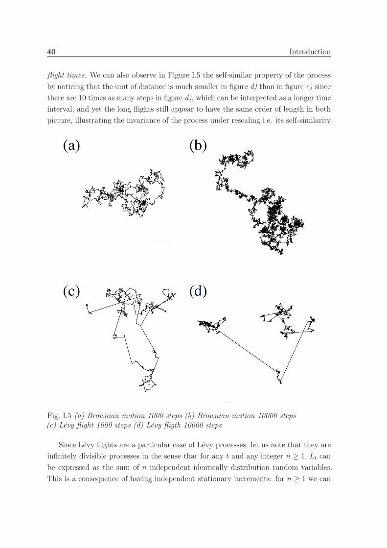
40 Introduction
flight times. We can also observe in Figure I.5 the self-similar property of the process
by noticing that the unit of distance is much smaller in figure d) than in figure c) since
there are 10 times as many steps in figure d), which can be interpreted as a longer time
interval, and yet the long flights still appear to have the same order of length in both
picture, illustrating the invariance of the process under rescaling i.e. its self-similarity.
Fig. I.5 (a) Brownian motion 1000 steps (b) Brownian motion 10000 steps(c) Lévy flight 1000 steps (d) Lévy fligth 10000 steps
Since Lévy flights are a particular case of Lévy processes, let us note that they are
infinitely divisible processes in the sense that for any t and any integer n ≥ 1, Lt can
be expressed as the sum of n independent identically distribution random variables.
This is a consequence of having independent stationary increments: for n ≥ 1 we can

I.2 Non-local diffusion equations 41
write explicitly:
Lt = Lt/n +[L2t/n − Lt/n
]+ · · ·+
[Lnt/n − L(n−1)t/n
]
where, thanks to iii) and iv), the [Lkt/n − L(k−1)t/n] are independent identically dis-
tributed random variables. As a result, we can express its characteristic function φ(t, k)
by the Lévy-Khintchine formulation (see e.g. [DSU08]) and, given the properties of
this particular process, we actually have
φ(t, k) = e−t|k|α
which will be of significant importance for the macroscopic description of non-local
diffusion.
I.2.3 Macroscopic description: the fractional heat equation
One way to derive the macroscopic equation for the density ρ(t, x) of a cloud of particles
undergoing Lévy flights is to generalise Einstein’s integral conservation relation (I.11)
to a general Lévy process Lt as:
ρ(t +∆t, x)− ρ(t, x) = E(ρ(t, x+ L∆t)− ρ(t, x)
)
which still expresses the idea that the evolution of the particle density ρ can be derived
from the average displacement of the particles. The derivation of the macroscopic
equation is equivalent to identifying the limit operator A:
A = lim∆t→0
1
∆tE(ρ(t, x+ L∆t)− ρ(t, x)
). (I.41)
This is the infinitesimal generator of the semigroup associated with the process Lt.
Namely, if we write Tt for the semigroup associated with Lt, defined as
Ttρ(t, x) = E(ρ(t, x+ Lt)
)
then the operator A can be equivalently defined as the infinitesimal generator of Tt
Aρ = limt→0
(Tt − 1)ρ
t.
42 Introduction
Moreover, the characteristic function of the process Lt is related to the semigroup Tt
via the Fourier transform (see e.g. [App09, Theorem 3.3.3]):
Ttρ(t, x) = F−1(φ(t, k)ρ(t, k)
).
In the case of Lévy flights φ(t, k) = e−t|k|α
hence
F(Ttρ(t, ·))(k) = e−t|k|
α
ρ(t, k)
which yields
F(Aρ(t, ·))(k) = lim
t→0
e−t|k|α − 1
tρ(t, k) = −|k|αρ(t, k).
The resulting diffusion equation, in Fourier variable, reads
∂tρ(t, k) = −|k|αρ(t, k). (I.42)
This is the fractional heat equation in Fourier variables [ARMAG00], [VTPV11],
[CHS12], [BC16]. It belongs to a wide class of PDE called non-local diffusion equa-
tions which model a variety of non-classical diffusion phenomena, including those we
are considering in this section.
I.2.3.0.1 Fractional Sobolev spaces and the fractional Laplace operator
In order to make sense of this equation in non-Fourier variable and define the frac-
tional Laplacian, the operator whose Fourier transform is (−A), we take a functional
analysis approach, in the spirit of [DPV12], and introduce the fractional Sobolev space
in Fourier variable:
Definition I.2.3. In Fourier variable, the fractional Sobolev space of order s ∈(0, 1): Hs(Rd), is the Hilbert space defined as
Hs(Rd) =u ∈ L2(Rd) :
∫
Rd
(1 + |ξ|2s)|u(ξ)|2 dξ <∞. (I.43)
I.2 Non-local diffusion equations 43
Note that, as is common in this framework, we have adopted the notation s for
the fractional order, which is related to the previous α of the Lévy flights as
s =α
2
and we will keep this notation here on in.
The non-Fourier version of this functional space is defined by the following proposition
from [DPV12, Section 3].
Proposition I.2.1. Consider s ∈ (0, 1). The Hilbert space Hs(Rd) coincides with the
fractional Sobolev space Hs(Rd) defined as
Hs(Rd) =u ∈ L2(Rd) :
∫∫
Rd×Rd
|u(x)− u(y)|2|x− y|d+2s
dx dy <∞. (I.44)
In particular, if we define the Gagliardo semi-norm [u]Hs(Rd) as
[u]Hs(Rd) =
( ∫∫
Rd×Rd
|u(x)− u(y)|2|x− y|d+2s
dx dy
)1/2
(I.45)
then we have∫
Rd
|ξ|2s∣∣u(ξ)
∣∣2 dξ = 1
2cd,s[u]
2Hs(Rd) (I.46)
where the constant cd,s is given by
cd,s =
(∫
Rd
1− cos(z1)
|z|d+2sdz
)−1
(I.47)
with z1 the first coordinate of z ∈ Rd.
This proposition expresses the link between a multiplication by |ξ|2s in Fourier
variable and the singular kernel 1/|x − y|d+2s. Let us give some details about this
relation which is crucial to understand non-local diffusion. We first notice, see [DPV12]
for details, that the constant cd,s satisfies for all ξ ∈ Rd:
(cd,s)−1|ξ|2s =
∫
Rd
1− cos(ξ · z)|z|d+2s
dz.

44 Introduction
Using this relation, we can prove the equivalence between the semi-norms (I.46) and
the equivalence of the functional spaces naturally follows. For u ∈ Hs(Rd) we write
∫
Rd
|ξ|2s|u(ξ)|2 dξ = cd,s
∫∫
Rd×Rd
1− cos(ξ · z)|z|d+2s
|u(ξ)|2 dz dξ
=cd,s2
∫∫
Rd×Rd
|eiξ·z − 1|2|z|d+2s
|u(ξ)|2 dz dξ
and the key step is to recognise the Fourier transform of a translation operator in the
integrand on the right-hand-side. As a consequence, we have
∫
Rd
|ξ|2s|u(ξ)|2 dξ = cd,s2
∫∫
Rd×Rd
∣∣F(u(z + ·))(ξ)− u(ξ)∣∣2
|z|d+2sdz dξ
=cd,s2
∫
Rd
∥∥∥F(u(z + ·)− u(·)
|z| d+2s2
)∥∥∥2
L2(Rd)dz
and with the Plancherel formula this is∫
Rd
|ξ|2s|u(ξ)|2 dξ = cd,s2
∫
Rd
∥∥∥u(z + ·)− u(·)|z| d+2s
2
∥∥∥2
L2(Rd)dz
=cd,s2
∫∫
Rd×Rd
|u(x)− u(y)|2|x− y|d+2s
dx dy
with the change of variables y = z + x.
This characterisation of the fractional Sobolev spaces paves the way for the integral
definition of the fractional Laplacian:
Definition I.2.4. For a function u ∈ S(Rd), the fractional Laplace operator(−∆
)sis defined as
(−∆
)su(x) = cd,sP.V.
∫
Rd
u(x)− u(y)
|x− y|d+2sdy (I.48)
where P.V. denote the Cauchy principal value. It is the inverse Fourier transform of
the multiplication by |ξ|2s:(−∆
)su(x) = F−1
(|ξ|2su(ξ)
). (I.49)

I.2 Non-local diffusion equations 45
The kernel 1/|x − y|d+2s is singular, hence the need for the principal value which
can be defined in this situation as
P.V.
∫
Rd
u(x)− u(y)
|x− y|d+2sdy = lim
ε→0
∫
|y−x|>ε
u(x)− u(y)
|x− y|d+2sdy
and we see that in order for this integral to make sense we need some regularity
on u and that is why we have given the definition of(− ∆
)sas an operator from
the Schwartz functional space – i.e. the space of rapidly decaying smooth functions,
where this regularity requirement is obviously satisfies – into L2(Rd). However, we can
broaden the domain of definition of(−∆
)sby expressing its link with the fractional
Sobolev spaces:
Proposition I.2.2. If u is in Hs(Rd) then
[u]2Hs(Rd) = 2c−1d,s
∥∥(−∆)s/2
u∥∥2L2(Rd)
. (I.50)
As a consequence, the fractional Laplacian(−∆
)scan naturally be defined as an
operator from Hs(Rd) into its dual space H−s(Rd). Note that the integral definition of(−∆
)semphasise the non-local nature of the operator since in order to determine
its action on a function u evaluated at a point x ∈ Rd, we integrate over the whole
space, hence the behaviour of u far away from x can influence the action of(− ∆
)s
at x: the operator is non-local.
We have just given four equivalent definitions of the fractional Laplacian:
• as an integro-differential operator of fractional order (I.48),
• as the inverse Fourier transform of a multiplication by |ξ|2s (I.49),
• as the infinitesimal generator of a symmetric 2s-stable Lévy process (I.41),
• as an operator that sends Hs(Rd) into its dual space H−s(Rd) (I.50).
We can also define(−∆
)sas a fractional power of the Laplace operator in the context
of functional calculus of sectorial operators, see [Hen81], or a Dirichlet-to-Neumann
operator for an appropriate family of PDE on a half-space [CS07], or via its relation
with Riesz potentials [CP16].
Fractional differential operators have been studied by scientists since the beginning of
differential calculus. Indeed, as soon as Leibniz and Newton founded differential calcu-
lus in the XVIIth century, de l’Hôpital wondered what would happen if the differential

46 Introduction
order was fractional which led some of the most celebrated mathematicians – includ-
ing Euler, Laplace, Lacroix, Abel, Fourier, Liouville, Riemann, Laurent, Hadamard,
Heavyside, Riesz and many others – to define various generalisations of classical deriva-
tives, study the physical and mathematical relevance of these operators and see if the
definitions are compatible with each other which, more often than not, was not the
case, as presented in [CT14].
The multitude of equivalent definitions of the fractional Laplacian illustrates the fact
that this operator arises naturally in many different fields of mathematics and, as
a consequence, it is not surprising that this operator has received a lot of attention
from the community, especially in recent years as the mathematical understanding of
confined plasma and turbulent fluid improves and the engineering challenges involved
in the confinement of plasma are closer and closer to their resolution.
The fractional Laplacian has many very interesting and useful properties. Although
we will not state all of them we refer to [BV16] and [Poz16] for a full review on the
subject.
As a linear operator on Hs(Rd), the fractional Laplacian is symmetric: for u and v in
Hs(Rd)
∫
Rd
u(−∆
)sv dx =
∫
Rd
v(−∆
)su dx. (I.51)
It actually realises the natural scalar product in the Hilbert space Hs(Rd) as illustrated
by (I.50). Moreover, it commutes with derivatives of integer order and with other
fractional Laplacians of any order. Futher, if we look at it as the infinitesimal generator
of a 2s-stable Lévy process, then it comes as no surprise that it is 2s-homogeneous in
the sense that for any λ ∈ R then
(−∆
)s[u(λx)
]= λ2s
(−∆
)s[u](λx) (I.52)
which expresses the self-similar property (I.40) of the underlying Lévy process.
Finally, let us mention that we can generalise the Poincaré inequality to a fractional
inequality using the fractional Laplacian, although the resulting inequalities are of
a very different nature since(− ∆
)sis a non-local operator. The generalisation
can be done in the same space where the classical Poincaré inequality holds, i.e. an
exponentially weighted L2 space, see [MRS11]. However, in the context of fractional
kinetic equations which we are about to present, it is more natural to look for a
Poincaré inequality in a L2 space with a polynomial weight. Such a generalisation was
I.2 Non-local diffusion equations 47
done in 2008 by I. Gentil and C. Imbert [GI08]. They took advantage of the relation
between the infinitesimal generator of a Lévy process and the measure associated with
the semigroup it generates in order to prove a modified logarithmic Sobolev inequality.
In the case of the fractional Laplacian, the measure µ associated with the semigroup
is explicitly µ( dx) = F (x) dx with
F (ξ) = Ce−|ξ|2s
2s (I.53)
where C is a normalising constant. The modified logarithmic Sobolev inequality
reads, for the fractional Laplacian
Theorem I.2.3. For all smooth positive functions u,
∫
Rd
u2F (x) dx−(∫
Rd
uF (x) dx
)2
≤∫∫
Rd×Rd
(u(x)− u(y)
)2
|x− y|d+2sF (x) dx dy
A proof of this particular case of I. Gentil and C. Imbert’s result can be found in
Chapter II.
Remark I.2.4. The fractional Laplacian is an example of a wider class of non-local
diffusion operators of the form
Au(x) =
∫
Rd
(u(x)− u(y)
)K(x, y) dy
for some singular kernel K, which are actually the object of study of I. Gentil and C.
Imbert in [GI08]. These non-local operators can also arise in the modelling of plasmas
of turbulent fluids when one considers more general Lévy processes in the microscopic
scale, instead of the particular case of the Lévy flights that we presented.
I.2.3.0.2 The fractional heat equation
We can now write the fractional heat equation in physical variables with initial
condition ρin:
∂tρ+
(−∆
)sρ = 0 (t, x) ∈ [0,+∞)× R
d
ρ(0, x) = ρin(x) x ∈ Rd.
(I.54)
We have seen that we can derive this equation from a Lévy flight model for the motion
of particles. Note, however, that we did not derive this non-local equation from a
48 Introduction
generalisation of Fourier’s argument. To understand why, recall that the basic idea
behind Fourier’s law is that in order to exit a ball B a particle must interact with
its boundary, hence we can derive the evolution of the particle density in B from the
interaction between the particles and the boundary ∂B as expressed in equation (I.1).
In the non-local framework, there seems to be a conceptual incompatibility between
the non-local behaviour of the process and the localised surface ∂B. As a consequence,
generalizing Fourier’s approach to the non-local diffusion case is a challenging issue.
Nevertheless, the fractional heat equation retains some of the properties of the heat
equation. For instance, since the fractional Laplacian generates a semi-group, we have
a fundamental solution Φs, solution of the evolution equation with initial condition
ρin(x) = δx=0, whose Fourier transform reads
Φs(t, k) = Ce−t|k|2s
where C is a normalising constant. As usually, we can construct general solution of
(I.54) by convolution with the fundamental solution
ρ(t, x) = ρin ∗ Φs(t, x).
Moreover, a simple energy bound shows that this is the unique weak solution of the
fractional heat equation in Hs(Rd): multiplying by ρ and integrating we have
d
dt
∫∫
Rd×Rd
ρ2 dx+ [ρ]2Hs(Rd) = 0.
Since the equation is linear the difference between two weak solutions satisfies (I.54)
with ρin ≡ 0 and the energy bound ensure that this solution stays null for all times if
it is in Hs(Rd).
I.2.4 Kinetic equations with heavy tailed equilibrium
We will consider two kinetic descriptions of the non-local diffusion processes, general-
isations of the Vlasov-linear relaxation equation (I.23) and the Vlasov-Fokker-Planck
equation (I.30).
One of the most crucial differences between classical and non-local diffusion is the ve-
locity equilibrium distribution. This distribution is a local Maxwellian distribution in
the classical case. In the non-local case however, as a consequence of the high energy
I.2 Non-local diffusion equations 49
levels and the long flights in the microscopic motion, their is much higher concentra-
tion of high-velocity particles and the equilibrium is heavy tailed in the sense that
it decays as a polynomial for high velocities instead of the exponential decay of the
Maxwellian. If we denote by F (v) this normalised equilibrium, it satisfies
F (v) ∼|v|≫1
1
|v|d+2s,
∫
Rd
F (v) dv = 1. (I.55)
The generalisation of the Vlasov-linear relaxation equation follows immediately, we
just replace the equilibrium in the collision operator by this heavy-tailed F and the
kinetic equation becomes:
∂tf + v · ∇xf = ρF − f (t, x, v) ∈ [0,∞)× R
d × Rd,
f(0, x, v) = fin(x, v) (x, v) ∈ Rd × R
d(I.56)
where ρ(t, x) =∫Rd
f dv.
To generalise the Fokker-Planck operator we introduce the Langevin equation with
a Lévy white noise: x = v(t)
v = −v(t) + L2st
(I.57)
where L2st is a symmetric 2s-stable Lévy process. Since the infinitesimal generator of
this process is the fractional Laplacian, the resulting kinetic equation is the fractional-
Vlasov-Fokker-Planck equation:
∂tf + v · ∇xf = ∇v · (vf)−
(−∆v
)sf (t, x, v) ∈ [0,∞)× R
d × Rd
f(0, x, v) = fin(x, v) (x, v) ∈ Rd × R
d.(I.58)
Taking the Fourier transform in velocity of the fractional Fokker-Planck operator, the
right-hand-side above, it is simple to solve for its equilibrium and recover the distribu-
tion F , defined in Fourier variables in (I.53), which indeed satisfies (I.55).
As we did in the classical case, we are interested in the diffusion limit of these
equations. Introducing the Knudsen number ε and a scaling adapted to (I.40) or
(I.52), namely
t′ = ε2st, x′ = εx

50 Introduction
the resulting rescaled equations take the form
ε2s∂tfε + εv · ∇xfε = L(fε) (t, x, v) ∈ [0,∞)× R
d × Rd
fε(0, x, v) = fin(x, v) (x, v) ∈ Rd × R
d.(I.59)
where L is either one of the previous linear operators. Since the scaling differs from
the classical case, we call anomalous diffusion limit the study of the behaviour of
fε when ε goes to 0. We will present separately the case of the Vlasov-linear relaxation
equation with heavy tailed equilibrium in section I.2.4.1 and for the fractional Vlasov-
Fokker-Planck equation in section I.2.4.2. Before that, however, let us notice that the
operators we consider both satisfy the dissipativity condition defined in Proposition
I.1.7 where the local Maxwellian M should be replaced by the heavy-tailed equilib-
rium F . The proof of this dissipativity is very similar to the classical case for the
heavy-tailed relaxation operator and varies a little for the fractional Fokker-Planck
and requires using the modified logarithmic Sobolev inequality of Theorem I.2.3. The
dissipativity of the operators ensures the system will converge to a state of velocity-
equilibrium as ε goes to 0 and eventually leads to the following a priori convergence
result, common to both cases .
Proposition I.2.5. Consider fin in L2F−1(Rd×Rd) and the weak solution fε of (I.59)
in L∞(0, T ;L2F−1(Rd × Rd)) for some time T > 0. Then
fε ρ(t, x)F (v) weak- ∗ in L∞(0, T ;L2F−1(Rd × R
d))
where ρ is the weak limit of ρε =∫Rd
fε dv.
I.2.4.1 Anomalous diffusion limit of a Vlasov-linear relaxation equation
The anomalous diffusion limit of the Vlasov-linear relaxation equation (I.56) was first
derived in 2008 by A. Mellet, S. Mischler and C. Mouhot in [MMM11] through a
Laplace-Fourier transform of the equation with respect to the time and space variables.
Their proof differs significantly from the classical case, in particular because the Fick
law (or Fourier law) fails so we cannot hope to derive the anomalous diffusion limit by
means of the current density. Instead, they approach consists in taking the Laplace-
Fourier transform of the equation which reads, with p the Laplace variable associated
with t, and k the Fourier variable of x:
ε2spfε − ε2sfin + εiv · kfε = ρεF − fε.

I.2 Non-local diffusion equations 51
Factorising appropriately and integrating with respect to v they get
ρε =
(∫
Rd
F (v)
1 + ε2sp+ εiv · k dv
)ρε +
(∫
Rd
ε2sfin1 + ε2sp+ εiv · k dv
)
and they were able to identify the limit of both terms to recover the fractional heat
equation. Although this method is remarkably efficient, the use of the Fourier trans-
form in the space variable is rather restrictive and forbids to look at space dependent
collision operator or, eventually, bounded domains. This led A. Mellet in 2010 to de-
velop a moment method for this anomalous diffusion limit in [Mel10] which we present
now.
Instead of taking Fourier or Laplace transforms, Mellet’s method focuses on the weak
formulation of the kinetic equation and consists in choosing a particular sub-class of
test functions through an auxiliary problem. The idea behind this method is that
since we want, in the limit as ε goes to 0, to identify ρ(t, x), we need to consider in the
weak formulation all test functions for t and x but we can choose how the test function
depends on the velocity as long as it does not conflict with the convergence when ε
tends to 0. Hence, we build an auxiliary problem through which we construct, from
ψ ∈ D([0, T )× Rd), a test function φε(t, x, v) which depends on the velocity variable
in an appropriate way and such that φε(t, x, v) tends to ψ(t, x) so that we can take
the limit in the weak formulation and recover the fractional heat equation on ρ.
Mellet’s moment method is fundamental to all the results we present in this thesis
so let us give more details on his auxiliary problem and the convergence of the weak
formulation.
I.2.4.1.1 Auxiliary problem
For a test function ψ ∈ D([0,+∞)× Rd) we construct φε(t, x, v) in L∞((0,+∞)×Rdv;L
2(Rdx)) as a solution of
φε − εv · ∇xφε = ψ(t, x). (I.60)
This equation is easily integrated and we have an explicit formula for φε:
φε(t, x, v) =
+∞∫
0
e−zψ(t, x+ εvz) dz.

52 Introduction
Futher, we see that φε is smooth, bounded in L∞ and also:
|φε(t, x, v)− ψ(t, x)| =∣∣∣∣+∞∫
0
e−z[ψ(t, x+ εvz)− ψ(t, x)
]dz
∣∣∣∣
≤ ε|v|‖ψ‖L∞((0,+∞)×Rd)
hence
φε(t, x, v) −→ε→0
ψ(t, x) uniformly with respect to t and x.
However, the convergence is not uniform in v but it is not an obstacle to the conver-
gence of the weak formulation because it satisfies
Lemma I.2.6. Consider ψ ∈ D([0,+∞)× Rd) and φε solution of (I.60). We have
∫
Rd
[φε(t, x, v)− ψ(t, x)
]F (v) dv −→
ε→00 uniformly with respect to t and x,
∫
Rd
[∂tφε(t, x, v)− ∂tψ(t, x)
]F (v) dv −→
ε→00 uniformly with respect to t and x.
Furthermore, ‖φε‖L2
F ((0,+∞)×Rd×Rd) ≤ ‖ψ‖L2F ((0,+∞)×Rd),
‖∂tφε‖L2F ((0,+∞)×Rd×Rd) ≤ ‖∂tψ‖L2
F ((0,+∞)×Rd).
I.2.4.1.2 Identifying the limit
The weak formulation of (I.56) on Q = [0,+∞) × Rd × Rd) with test function
φ(t, x, v) reads
∫∫∫
Q
[fε
(ε2s∂tφ+ εv · ∇xφ− φ
)+ ρεFφ
]dt dx dv = ε2s
∫∫
Rd×Rd
finφ(0, x, v) dx dv.
I.2 Non-local diffusion equations 53
Taking the solution φε of the auxiliary problem as test function, we see that we have
(since F is normalised)
∫∫∫
Q
[fε
(εv · ∇xφε − φε
)+ ρεFφε
]dt dx dv
=
∫∫
[0,+∞)×Rd
ρε
∫
Rd
[φε(t, x, v)− ψ(t, x)
]F (v) dt dx dv.
Introducing the operator Lε defined as
Lε(ψ) = ε−2s
∫
Rd
[φε(t, x, v)− ψ(t, x)
]F (v) dv (I.61)
the weak formulation becomes∫∫
[0,+∞)×Rd
(∫
Rd
fε∂tφε dv + ρεLε(ψ))dt dx =
∫∫
Rd×Rd
fin(x, v)φε(0, x, v) dx dv. (I.62)
Note that this weak formulation does not identify fε as the solution of the heavy-tailed
Vlasov-linear relaxation equation (I.56) because it is only satisfied for a particular sub-
class of test functions. However, the solution of (I.56) does satisfy (I.62) for all φεsolution of (I.60) and the structure of a diffusion equation appears where Lε is a kinetic
approximation of a non-local diffusion operator.
The rest of the proof consists in taking the limit as ε goes to zero in this formulation.
The convergence of the partial derivative with respect to time and the initial condition
follows from the a priori estimates and the bounds on φε. We focus on Lε. From the
explicit expression of φε we have
Lε(ψ) = ε−2s
∫
Rd
+∞∫
0
e−z[ψ(t, x+ εvz)− ψ(t, x)
]F (v) dz dv.
The convergence of this operator towards the fractional Laplacian rests upon the
relation between F and the singular kernel of(−∆
)s. Indeed, we know that F (v) ∼
κ0/|v|d+2s for large v and some κ0 > 0, so the change of variable w = εvz yields
54 Introduction
formally
Lε(ψ) = ε−2s
∫
Rd
+∞∫
0
e−z[ψ(t, x+ w)− ψ(t, x)
]F(wεz
) 1
|εz|d dz dw
∼ε≪1
ε−2s
∫
Rd
+∞∫
0
e−z[ψ(t, x+ w)− ψ(t, x)
](εz)d+2s
|w|d+2s
1
|εz|d dz dw
∼ε≪1
∫
Rd
+∞∫
0
z2se−zψ(t, x+ w)− ψ(t, x)
|w|d+2sdz dw
−→ε→0
−κ(−∆x
)sψ(t, x)
where the constant κ is given by
κ =κ0cd,s
+∞∫
0
z2se−z dz.
The rigorous proof of this limit can be done by splitting the integral over v in two:
|v| ≥ C∪|v| ≤ C and showing that the integral over small velocity vanishes while,
in the integral over large velocities, the equilibrium F converges to the singular kernel
κ0/|v|d+2s. See [Mel10] for more details.
Put together, the limit of (I.62) identifies the limit ρ of fε/F (v) as solution of
∫∫
[0,+∞)×Rd
ρ(∂tψ − κ
(−∆x
)sψ)dt dx =
∫
Rd
ρinψ(0, x) dx
for all ψ ∈ D([0,+∞)×Rd) and the uniqueness of weak solution of the fractional heat
equation in Hs ensure that ρ is this unique solution.
I.2.4.2 Anomalous diffusion limit of a fractional Vlasov-Fokker-Planck
equations
The anomalous diffusion limit of the fractional Vlasov-Fokker-Planck equation (I.58)
was derived in 2012 by myself, A. Mellet and K. Trivisa [CMT12] 1. Although the
limit can be obtained through a Fourier method we will focus here a moment method
1Erratum for [CMT12]: In the proof of [CMT12, Proposition 2.1] the Poincaré inequality of[MRS11] does not hold, one needs to use instead the modified log-Sobolev inequality of [GI08]. Theresults remains unchanged.

I.2 Non-local diffusion equations 55
for the same reasons as before. Building on Mellet’s idea, we want to construct a
particular sub-class of test functions in order to isolate the diffusion phenomena in
the weak formulation, creating an adapted kinetic approximation of the fractional
heat equation, and then take the limit in this approximation. However, this sub-class
of test functions will take a different form for the fractional Vlasov-Fokker-Planck
equation because we already have an explicit non-local operator in the collision model,
acting on the velocities. As a consequence, the purpose of the auxiliary problem will be
to identify a relevant relation between the position and the velocity variable through
which we can exhibit how the non-local phenomena in the behaviour of the velocities
of particles in the microscopic scale (c.f. the Langevin equation with Lévy white noise
(I.57)) results in non-local behaviour for the particle density ρ at the macroscopic
scale.
I.2.4.2.1 Auxiliary problem
To build the auxiliary problem, we take advantage of the particular structure the
fractional Vlasov-Fokker-Planck equation exhibits when we take its Fourier transform
in position and velocity. Indeed, with Fourier variables p and ξ for x and v respectively,
the rescaled equation reads
ε2s∂tfε +(εk − ξ) · ∇ξfε = −|ξ|2sfε
which is a scalar-hyperbolic equation whose characteristic lines are given by the term
(εk − ξ) · ∇ξ. This motivates the following auxiliary problem to construct φε from
ψ ∈ D([0,+∞)× Rd):
εv · ∇xφε − v · ∇vφε = 0 (t, x, v) ∈ [0,+∞)× R
d × Rd
φε(t, x, 0) = ψ(t, x) (t, x) ∈ [0,+∞)× Rd.
(I.63)
In this setting, we have an explicit solution for φε which is
φε(t, x, v) = ψ(t, x+ εv).
which is smooth in all variables. Moreover
φε(t, x, v) −→ε→0
ψ(t, x) in D([0,+∞)× Rd).
so it will does not conflict with the convergence of the associated weak formulation.
56 Introduction
I.2.4.2.2 Identifying the limit
The weak formulation of (I.58) on Q = [0,+∞)×Rd×Rd with test function φ reads
∫∫∫
Q
fε
(ε2s∂tφ+ εv · ∇xφ− v · ∇vφ−
(−∆v
)sφ)dt dx dv
= ε2s∫∫
Rd×Rd
finφ(0, x, v) dx dv.
With the test function φε above, it becomes
∫∫∫
Q
fε
(ε2s∂tφε −
(−∆v
)sφε
)dt dx dv = ε2s
∫∫
Rd×Rd
finφε(0, x, v) dx dv
and since(−∆
)sis 2s-homogeneous (I.52) we have
(−∆v
)sφε =
(−∆
)s[φ(t, x+ εv)
]= ε2s
(−∆
)s[ψ(t, ·)
](x+ εv).
Hence, the weak formulation can be written as
∫∫∫
Q
fε
(∂tψ(t, xεv)−
(−∆
)s[ψ(t, ·)
](x+ εv).
)dt dx dv =
∫∫
Rd×Rd
finψ(0, x+ εv) dx dv
and the rest of the proof consists in taking the limit as ε goes to 0. Notice that
we cannot write explicitly an operator Lε independent of v as we did in the linear
relaxation case to approximate the fractional Laplacian. Nevertheless, the strong
convergence of φε towards ψ(t, x) ensures that
∫∫∫
Q
fε(−∆
)s[ψ(t, ·)
](x+ εv) dt dx dv −→
ε→0
( ∫∫
[0,T )×Rd
ρ(−∆x
)sψ dt dx
)(∫
Rd
F (v) dv
)
so we recover the fractional heat equation in the limit
∫∫
[0,+∞)×Rd
ρ(∂tψ −
(−∆x
)sψ)dt dx =
∫
Rd
ρinψ(0, x) dx
for all ψ ∈ D([0,+∞)× Rd).

I.3 Confining a diffusion process 57
I.3 Confining a diffusion process
Now that we have presented the different models of local and non-local diffusion phe-
nomena at the microscopic, the kinetic and the macroscopic scale and seen the relations
between them, we turn to the main focus of this thesis: the confinement of diffusion
processes.
We consider two types of confinement: "soft" confinement with an external electric
field and "hard" confinement with a bounded domain. Of course, there are other ways
to confine a diffusion process, for instance with a self-consistent electric field (given by
a Poisson equation), or we could also consider the free boundary problem which may
exhibit a confinement resulting from the balance of attracting and repulsing forces
inside the fluid.
We start this section with the electric field case, introducing the problem and giving
some results in the classical diffusion setting. Next, we consider bounded domains,
introduce the classical macroscopic boundary conditions for the heat equation, and
present some of the associated results before moving on to the kinetic boundary con-
ditions that Maxwell introduced in the late XIXth century. Then, building from the
classical diffusion limits, we show how we can recover the macroscopic boundary con-
ditions from the kinetic ones. Finally, we investigate the confinement of non-local
diffusion processes and look at this problem from both a microscopic and a macro-
scopic point of view, presenting some of the most recent results on that subject.
I.3.1 External electric field
Let us consider a rarefied gas, or a fluid, near equilibrium and subject to an external
electric field E(t, x) which derives from a electric potential Φ: E = ∇xΦ. At the
microscopic scale, the field affects the velocity of the particles and hence modifies the
Langevin description (I.29) of the evolution of (x(t), v(t)) the position and velocity of
a given particle, which becomes
x = v(t)
v = E(t, x)− µv(t) +DBt
(I.64)
where µ and D, the viscosity and diffusion constants, will be assumed equal to 1 from
now on, and Bt is a Wiener process. We can see here that, for example, if the vector E
is oriented towards the origin, then the field discourages particles from moving away
from the origin, hence the term "soft" confinement.

58 Introduction
The resulting kinetic equation is a linear Vlasov-Fokker-Planck with an electric field:
∂tf + v · ∇xf + E(t, x) · ∇vf = ∇v · (vf) + ∆vf (t, x, v) ∈ [0, T )× R
d × Rd
f(0, x, v) = fin(x, v) (x, v) ∈ Rd × R
d.
(I.65)
This equation can be interpreted as a perturbation of the linear Vlasov-Fokker-Planck
equation (I.30) in the sense that the collision operator is perturbed by the electric field
and becomes
LFP,Ef = ∇v ·[(v − E(t, x))f
]+∆vf.
If the perturbation is "nice enough", namely if E is in L∞((0, T ) × Rd) – note that
E(t, x) ∈ Rd so that when we say E is in some functional space F we mean that if
we write E(t, x) = (E1(t, x), . . . , Ed(t, x)) then each of the component Ei(t, x) is in F– then it does not affect the fundamental properties of the equation and we can prove
similar existence and regularity results as in the unperturbed case, as was done for
instance in [BD95] or [EGM10]:
Proposition I.3.1. Consider T > 0, E ∈ L∞((0, T )× Rd) and fin ∈ L2
M−1(Rd × Rd)
such that
fin ≥ 0 and∫∫
Rd×Rd
(1 + |v|2 + ln fin)fin dx dv <∞
then (I.65) has a weak solution f ∈ C([0, T );L2M−1(Rd × Rd) that satisfies
f ≥ 0 and for all t ∈ [0, T ) :
∫∫
Rd×Rd
(1 + |v|2 + ln f)f dx dv <∞.
Advection-diffusion limit
Let us derive the macroscopic equation on ρ that follows from this perturbed Vlasov-
Fokker-Planck equation. Since we are in the classical case, we use rescaling
t′ = ε2t, x′ = εx
where ε is the Knudsen number (I.34). In order to investigate the limit as ε goes to 0,
we need to know how E rescales with ε. Since E derives from a potential Φ, we see
I.3 Confining a diffusion process 59
that
E(ε2t, εx) = ∇x
[Φ(ε2t, εx)
]= ε∇xΦ(ε
2t, εx) = εE(t′, x′). (I.66)
Hence, the rescaled kinetic equation reads
ε2∂tfε + εv · ∇xfε + εE · ∇vfε = ∇v · (vfε) + ∆vfε on [0, T )× Rd × R
d
fε(0, x, v) = fin(x, v) on Rd × R
d.(I.67)
We can investigate the behaviour of fε as ε goes to 0 by adapting the method developed
in Section I.1.3.4 for the case without the electric field:
Proposition I.3.2. Consider T > 0 and fin satisfying the assumption of Proposition
I.3.1. Then the solution of the rescaled equation (I.67) converges towards ρ(t, x)M(v)
weak-∗ in L∞([0, T );L2M−1(Rd×Rd)) where M is the local Maxwellian equilibrium (I.31)
and ρ is the weak limit of ρε =∫Rd
fε dv.
We also retain uniform control on the energy
Eε(t, x) =∫∫
Rd×Rd
( |v|22
+ ln fε
)fε dx dv.
Details on this a priori estimates can be found in [PS00] or [EGM10], and also in
Chapter II of this thesis. We focus here on identifying the limit. To that end, we
integrate the equation to derive the continuity equation for the density ρε:
∂tρε +1
ε∇xjε = 0
where jε is now the current density
jε =
∫
Rd
vfε dv.
The a priori estimates ensure that 1εjε converges, we want to identify its limit. Multi-
plying (I.67) by v/ε and integrating we have in the sense of distributions
ε∂tjε +∇x
∫
Rd
v ⊗ vfε dv − dE(t, x)ρε = −dεjε.
60 Introduction
We know that the second term on the left-hand-side will tend to −∇x · (ρId) and the
bounds on ρε ensure that the third term on the left-hand-side will tend to −dEρ hence
d
εjε → d∇xρ+ dE(t, x)ρ
and together with the continuity equation we get the advection-diffusion limit of the
Vlasov-Fokker-Planck equation with an external electric field:
∂tρ−∇x · (∇xρ+ E(t, x)ρ) = 0 (t, x) ∈ [0, T )× R
d
ρ(0, x) = ρin(x) x ∈ Rd
(I.68)
As expected, this equation models the evolution of ρ under the effects of a diffusion
and an advection resulting from the electric field.
I.3.2 Bounded domains
We consider a bounded domain Ω ⊂ Rd and consider a fluid confined in that domain.
We will always assume that Ω is smooth in the sense that there exists a smooth function
ξ : Rd 7→ R such that
Ω =x ∈ R
d : ξ(x) < 0
and ∂Ω =x ∈ R
d : ξ(x) = 0
and we also assume that ∇xξ(x) 6= 0 for all |x| ≪ 1 so that we can define the outward
normal vector n(x) = ∇xξ(x)/|∇xξ(x)| everywhere on the boundary.
I.3.2.1 Macroscopic boundary conditions for classical diffusion equations
Let us consider the heat equation in Ω:
∂tρ = ∆ρ (t, x) ∈ [0, T )× Ω
ρ(0, x) = ρin(x) x ∈ Ω.(I.69)
In order to close this problem we need to describe how ρ behaves on the boundary.
There are two fundamental ways to do this, either impose the value of ρ on the bound-
ary, or the value of its normal derivative. We focus on the homogeneous conditions:
I.3 Confining a diffusion process 61
• Homogeneous Dirichlet boundary condition
ρ(t, x) = 0 (t, x) ∈ [0, T )× ∂Ω (I.70)
• Homogeneous Neumann boundary condition
∇xρ(t, x) · n(x) = 0 (t, x) ∈ [0, T )× ∂Ω. (I.71)
We can build solutions to the initial-boundary-value problems (I.69)-(I.70) and (I.69)-
(I.71) using the eigenvalues of the Laplacian and the associated orthonormal basis
of L2(Ω), see e.g. [Eva10] or [Tay11]. Note that in the Neumann case, we have
conservation of mass since the boundary is reflective, as we can see easily by integrating
the equation, but that is not necessarily true in the Dirichlet case. In both cases, we
have uniqueness of solution, in H10 (Ω) for Dirichlet, and H1(Ω) for Neumann. Indeed,
a simple energy estimate shows
d
dt
∫
Ω
ρ(t, x)2 dx+
∫
∂Ω
∣∣∇xρ∣∣2 dx = 0.
Using the Poincaré inequality, it follows that the H1-norm decreases, hence the unique-
ness since the equation is linear. Moreover, the solutions satisfy a remarkable property:
the maximum principle, which illustrates the diffusive effect of the equation by the
fact that the maximum value of the ρ(t, x) can only be attained on the boundary or
by the initial value:
Proposition I.3.3. Let ρ be a solution of (I.69) with either Dirichlet or Neumann
boundary condition in C([0, T )× Ω) ∩ C2((0, T )× Ω) then
sup[0,T )×Ω
ρ(t, x) = maxsupΩ
ρ(0, x), sup[0,T )×∂Ω
ρ(t, x)
and we refer to [Tay11] or [Eva10] for more a more detailed analysis of these
equations.
I.3.2.2 Kinetic boundary conditions
Let us consider the linear Vlasov-Fokker-Planck equation on Ω:
∂tf + v · ∇xf = ∇v · (vf) + ∆f (t, x, v) ∈ [0, T )× Ω× R
d
f(0, x, v) = fin(x, v) (x, v) ∈ Ω× Rd.
(I.72)

62 Introduction
Here again, we need to specify how f behaves on the boundary to which end we
introduce the oriented set:
Σ± = (x, v) ∈ Σ;±n(x) · v > 0 with Σ = ∂Ω× Rd (I.73)
where n(x) is the outgoing normal vector and we denote by γf the trace of f on
R+ × ∂Ω × Rd. The boundary conditions then take the form of a balance between
the values of the traces of f on these oriented sets γ±f := 1Σ±γf . Maxwell identified
in [Max79] three fundamental interactions between the cloud of particles and the
boundary which give rise to the following boundary conditions:
• The absorption boundary condition : for all (x, v) ∈ Σ−
γ−f(t, x, v) = 0 (I.74)
• The local-in-velocity reflection operator called specular reflection: for all (x, v) ∈Σ−
γ−f(t, x, v) = γ+f(t, x,Rx(v)
)(I.75)
where Rx(v) = v − 2(n(x) · v
)n(x) which is illustrated in Figure I.6.
• The non-local in velocity reflection operator called diffusion : for all (x, v) ∈ Σ−
γ−f(t, x, v) =M(v)
∫
Σx+
γ+f(t, x, w)|n(x) · w| dw (I.76)
where M is the Gaussian equilibrium (I.31) with the normalising assumption
∫
Σx−
M(w)|w · n(x)| dw = 1.
The first one models the absorption of the particles by the boundary, the second
expresses the reflection of the particle that bounces back with a reflected velocity
and the third is when the boundary diffuses back into the domain. For a reflective
boundary, the most physically relevant model for the interaction would be a linear
combination of specular reflection and diffusion, i.e. for some θ ∈ (0, 1):
γ−f(t, x, v) = θγ+f(t, x,Rx(v)
)+ (1− θ)M(v)
∫
Σx+
γ+f(t, x, v)|n(x) · v| dv
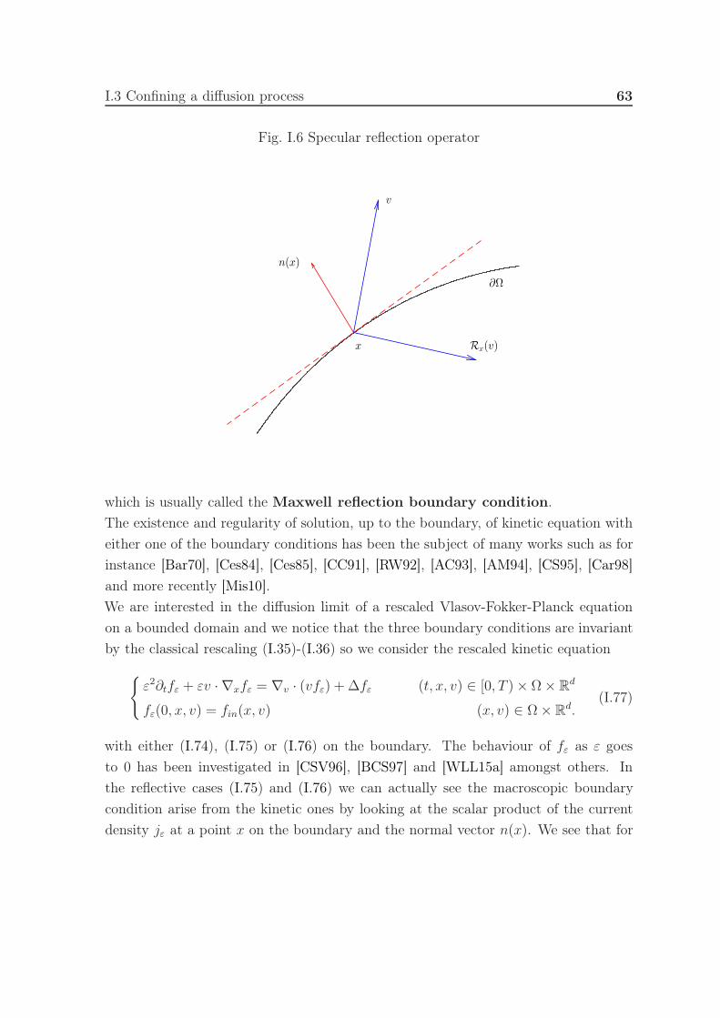
I.3 Confining a diffusion process 63
Fig. I.6 Specular reflection operator
v
Rx(v)x
n(x)
∂Ω
which is usually called the Maxwell reflection boundary condition.
The existence and regularity of solution, up to the boundary, of kinetic equation with
either one of the boundary conditions has been the subject of many works such as for
instance [Bar70], [Ces84], [Ces85], [CC91], [RW92], [AC93], [AM94], [CS95], [Car98]
and more recently [Mis10].
We are interested in the diffusion limit of a rescaled Vlasov-Fokker-Planck equation
on a bounded domain and we notice that the three boundary conditions are invariant
by the classical rescaling (I.35)-(I.36) so we consider the rescaled kinetic equation
ε2∂tfε + εv · ∇xfε = ∇v · (vfε) + ∆fε (t, x, v) ∈ [0, T )× Ω× R
d
fε(0, x, v) = fin(x, v) (x, v) ∈ Ω× Rd.
(I.77)
with either (I.74), (I.75) or (I.76) on the boundary. The behaviour of fε as ε goes
to 0 has been investigated in [CSV96], [BCS97] and [WLL15a] amongst others. In
the reflective cases (I.75) and (I.76) we can actually see the macroscopic boundary
condition arise from the kinetic ones by looking at the scalar product of the current
density jε at a point x on the boundary and the normal vector n(x). We see that for

64 Introduction
specular reflections
jε(t, x) · n(x) =∫
Σx+
γ+fεv · n(x) dv +∫
Σx−
γ−fεv · n(x) dv
=
∫
Σx+
γ+fε|v · n(x)| dv −∫
Σx−
γ+fε(x,Rx(v))v · n(x) dv
=
∫
Σx+
γ+fε|v · n(x)| dv −∫
Σx+
γ+fε(x, w)Rx(w) · n(x) dw
= 0
since Rx(w)·n(x) = −w ·n(x) as a direct consequence of the definition of Rx. Similarly
for diffusive boundary conditions:
jε(t, x) · n(x) =∫
Σx+
γ+fεv · n(x) dv +∫
Σx−
M(v)v · n(x) dv∫
Σx+
γ+fεw · n(x) dw
= 0
thanks to the normalising assumption on M . Hence, we have in both cases
jε(t, x) · n(x) = 0 ∀(t, x) ∈ [0, T )× ∂Ω.
Since we know that 1εjε → ∇xρ, it follows that both the specular reflection and the
diffusion boundary conditions give rise to the homogeneous Neumann condition on ρ
in the diffusion limit.
I.3.2.3 Boundary conditions for non-local diffusion equations
If we consider the fractional heat equation on a domain Ω
∂tρ−
(−∆
)sρ = 0 (t, x) ∈ [0, T )× Ω
ρ(0, x) = ρin(x) x ∈ Ω(I.78)
then it is not obvious, from a PDE point of view, what kind of boundary condition
we should consider in order to close this problem. Indeed, because of the non-local
nature of the fractional Laplacian, a Dirichlet or a Neumann boundary condition on
∂Ω would result in an ill-posed problem since these conditions are local in space.
The problem of confining of non-local diffusion processes arose first in the field of

I.3 Confining a diffusion process 65
Probability theory with the issue of confining a stable Lévy process to a bounded
domain, which was the subject of many works such as [Sil74], [Kom95], [CK02] or
[BBC03]. From a symmetric 2s-stable Lévy process Lt, K Bogdan K. Burdzy and Z.
Q. Chen define in [BBC03] three types of confined processes: the killed process Lkillt ,
the censored process Lcent and the reflected process Lref
t .
To define these processes we manipulate the associated Dirichlet form. Dirichlet forms
are powerful tools, initially introduced in the field of Potential theory in the 1950s
it was discovered in the 1970s that they can be directly related to certain random
processes and, consequently, that they constitute a extremely useful link between
probabilistic and analytic considerations. They have received a lot of attention and
we refer for instance to [MMR92] for a comprehensive introduction of the subject. In
the case of a Lévy flight Lt, the associated Dirichlet form is a pair (E ,F) of a bilinear
form E and a dense subspace F of L2(Rd) such that if A is the infinitesimal generator
of the semigroup associated with Lt (c.f. Section I.2.3) then for any u and v in L2(Rd):
E(u, v) = 〈−Au, v〉
where 〈·|·〉 is the scalar product on L2(Rd), and F is the domain of definition of E . In
this particular case, using the results we presented as the beginning of Section I.2.3,
we see immediately that the Dirichlet form associated with Lévy flights is (E , Hs(Rd))
where E is the scalar product on the homogeneous Sobolev space Hs(Rd)
E(u, v) = 1
2cd,s
∫∫
Rd×Rd
(u(x)− u(y)
)(v(x)− v(y)
)
|x− y|d+2sdx dy.
Now, the construction of the killed process Lkillt is the most straightforward: we add a
coffin state ∂ to Rd and define the exit time
tΩ = inft > 0 : Wt /∈ Ω.
The killed process Lkillt is then defined as
Lkillt =
Lt t < tΩ
∂ t ≥ tΩ.
It is exactly the Lévy flight killed upon leaving Ω. Its Dirichlet form (Ekill,FkillΩ ) is
simply the Dirichlet form of the Lévy flight restricted to functions that are 0 almost

66 Introduction
everywhere outside Ω:
FkillΩ = u ∈ Hs(Rd) : u = 0 a.e. on R
d \ Ω
Ekill(u, v) =1
2cd,s
∫∫
Ω×Ω
(u(x)− u(y)
)(v(x)− v(y)
)
|x− y|d+2sdx dy +
∫
Ω
u(x)v(x)κΩ(x) dx
where κΩ is the killing measure given by
κΩ(x) = cd,s
∫
Rd\Ω
1
|x− y|d+2sdy. (I.79)
To construct the censored process Lcent we want to forbid any long flights ending outside
the domain and only kill the process if it reaches the boundary through a continuous
path, unlike the killed process who enters the coffin state any time it goes outside of
Ω. This can be done by the Ikeda-Nagasawa-Watanabe piecing together procedure
[INW66], the idea is to check, at exit time tΩ, if the process left the domain as a result
of a continuous path, in which case we kill the process with the coffin state, or if it
left the domain as a result of a long flight in which case we start again with a new
Lévy process initiated at Lt−Ω at time tΩ. The resulting process is then confined to
the domain Ω and reads as a juxtaposition of killed processes as defined above. K.
Bogdan, K. Burdzy and Z.-Q. Chen gave an equivalent construction of this process
in [BBC03] through a Dirichlet form argument and they showed that the associated
form (E cen,F cenΩ ) is
F cenΩ = Hs(Ω) :=
u ∈ L2(Ω) :
∫∫
Ω×Ω
(u(x)− u(y)
)2
|x− y|d+2sdx dy <∞
E cen =1
2cd,s
∫∫
Ω×Ω
(u(x)− u(y)
)(v(x)− v(y)
)
|x− y|d+2sdx dy.
We can see, in this Dirichlet form, that forbidding any long flights ending outside
the domain comes down to reducing the domain of integration to Ω, hence making
"impossible" any long jumps that would result in leaving the domain.
Finally, the reflected process is basically a censored process that is not killed upon
leaving the domain, instead it is reflected back inside the domain by juxtaposing cen-
sored processes. One of the fascinating results of K. Bogdan, K. Burdzy and Z.-Q.
Chen is that when 0 < s < 1/2, the reflected and the censored processes are essen-

I.3 Confining a diffusion process 67
tially identical, which means that the probability of reaching the boundary through a
continuous path is 0. We will see in the chapters of this thesis that the case s = 1/2
is indeed critical in many situations.
The macroscopic confinement of non-local diffusion processes with PDE tools has re-
ceived more and more attention in recent years, often building from the probabilistic
point of view we just presented. Like at the microscopic scale, there are different ways
to add a boundary condition to the fractional heat equation in order to generalise the
homogeneous Dirichlet condition. The first method, which may seem the more natu-
ral from an Analysis of PDE point of view, is to impose the condition on the whole
complementary of the domain:
ρ(t, x) = 0 (t, x) ∈ [0, T )×(Rd \ Ω
).
This was the subject, for instance, of [FKV13] by M. Felsinger, M. Kassmann and P.
Voigt and also [ROS14] by X. Ros-Oton and J. Serra. They proved that the problem
with this boundary condition is well-posed and it actually corresponds to the killed
process W kt since it basically comes down to looking for a solution ρ of (I.78) in Hs(Rd)
such that ρ ≡ 0 on the complementary of Ω.
Another way to generalise the homogeneous Dirichlet condition is to define a new
operator that does not involve the values of ρ outside the domain. This operator is
called the regional fractional Laplacian(− ∆Ω
)s. It was introduced by Q.-Y. Guan
and Z.-M. Ma in [GM06] and it is defined (for a smooth convex domain) as
(−∆Ω
)sρ(x) = cd,sP.V.
∫
Ω
u(x)− u(y)
|x− y|d+2sdy
which corresponds to the censored process W cent . Since this operator confines the
non-local behaviour inside the domain, it is actually compatible with local-in-position
boundary conditions such as (I.70) and (I.71). There has been a growing series of work
on that subject as for instance [GM05], [Gua06], [CKS09], [MY15], [War15], [War16].
Note that when considering reflective boundary conditions such as (I.71), the under-
lying process would be the reflected one. These papers show well-posedness of the
equation and some results on the regularity of the solution up to the boundary.
There is a another remarkable approach to the problem of finding a reflective
boundary condition for the fractional heat equation, which was presented by S. DiP-

68 Introduction
ierro, X. Ros-Oton and E. Valdinoci in [DROV17]. They propose a non-local Neumann
condition in the form of an operator Ns defined for x ∈ Rd \ Ω as
Nxρ(x) = cd,s
∫
Ω
u(x)− u(y)
|x− y|d+2sdy. (I.80)
They prove in [DROV17] that the associated Neumann problem
(−∆
)sρ = f x ∈ Ω
Nxρ = 0 x ∈ Rd \ Ω
with f ∈ L2(Ω), and the fractional heat equation (I.78) with (I.80) are both well-posed
and prove some properties on the solution of the heat equation like conservation of
mass, decreasing energy and convergence to a steady state in long-time. The proba-
bilistic interpretation of their operator is a variation on the censored process. Morally,
their process is a juxtaposition of killed processes in such a way that when the parti-
cles jumps at a point x outside Ω, the process starts again from a point y inside the
domain where y is chosen randomly with probability distribution 1/|x− y|d+2s.

I.4 List of works presented in this thesis and perspectives 69
I.4 List of works presented in this thesis and perspec-
tives
In this thesis, we are interested in deriving confined non-local diffusion equations from
kinetic equations with a fractional Fokker-Planck collision operator.
Chapter II: Anomalous diffusion limit with an external electric field
based on [ASC16], joint work with P. Aceves-Sànchez
In this chapter, we consider the fractional Vlasov-Fokker-Planck equation with 1/2 ≤s ≤ 1 and an external field E(t, x):
∂tf + v · ∇xf + E · ∇vf = ∇v · (vf)−
(−∆v
)sf in [0, T )× R
d × Rd
f(0, x, v) = fin(x, v) in Rd × R
d.
We first show a result of existence of weak solutions before introducing, in the spirit
of Section I.2.4, the anomalous scaling
t′ = ε2s, x′ = εx. (I.81)
We show that if E satisfies the precise scaling property (which can be thought of as a
fractional version of (I.66)):
E(ε2st, εx) = ε2s−2E(t′, x′)
then in the limit as ε goes to 0, fε will tend to ρ(t, x)F (v) where ρ satisfies a fractional
advection-diffusion equation
∂tρ+∇x ·
(Eρ) +
(−∆
)sρ = 0 (t, x) ∈ [0, T )× R
d
ρ(0, x) = ρin(x) x ∈ Rd.
(I.82)
We conclude the chapter by focusing on the critical cases s = 1/2 and s = 1 and show-
ing that, up to minor modifications, our method for deriving the fractional advection-
diffusion equations also works in the critical cases.
Perspectives
The results presented in this chapter can be interpreted as a first step towards the
anomalous diffusion limit of a Vlasov-Fokker-Planck equation with a Poisson potential.

70 Introduction
We present some of the difficulties that arise when we consider an electric field in the
kinetic equation and exhibit a sufficient (although a priori not optimal) regularity
needed for that field in order to take the diffusion limit.
Note in particular, that the scaling property (I.66) does not seem compatible, at first
sight, with a classical Poisson equation of the form
E(t, x) = ∇xΦ, −∆Φ = ρ.
As a consequence, if we want to look at a self-consistent electric field generated by the
charged particles in a plasma and derive a fractional advection-diffusion equation – i.e.
if we want to generalise the results of [PS00], [Gou05] or [EGM10] to the fractional
case – then we should probably start by looking for a relevant generalisation of the
Poisson equation that ensures the appropriate scaling property for E.
Chapter III: Anomalous diffusion limit in bounded domains
based on [Ces16]
We consider the fractional Vlasov-Fokker-Planck equation on a smooth convex bounded
domain Ω
∂tf + v · ∇xf = ∇v · (vf)−
(−∆v
)sf in [0, T )× Ω× R
d
f(0, x, v) = fin(x, v) in Ω× Rd.
Since the non-local operator acts solely on the velocity variable, we can consider classi-
cal kinetic boundary condition on the spatial boundary ∂Ω. For instance, we consider
either absorption boundary condition
γ−f(t, x, v) = 0 on [0, T )× Σ−
where Σ− = (x, v) : x ∈ ∂Ω, v · n(x) < 0 as introduce in Section I.3.2.2, or the
specular reflection boundary condition
γ−f(t, x, v) = γ+f(t, x,Rx(v)
)on [0, T )× Σ−
where Rx(v) = v − 2v · n(x).We establish the anomalous diffusion limit of these problems. Introducing an anoma-
lous scaling equivalent to (I.81), we prove a priori estimates in both cases from which
we deduce the weak convergence of fε to ρ(t, x)F (v). In the absorption case, we

I.4 List of works presented in this thesis and perspectives 71
identify ρ as the solution of the fractional heat equation with a Dirichlet boundary
condition extended to the whole complementary of the domain
∂tρ−(−∆x
)sρ = 0 in [0, T )× Ω
ρ(0, x) = ρin(x) x ∈ Ω
ρ(t, x) = 0 in [0, T )×(Rd \ Ω
).
Note that in this PDE, the fractional Laplacian is to be understood as acting on the
extension of ρ by 0 outside the domain.
In the specular reflection case, we show that the boundary condition affects the diffu-
sion process of the macroscopic density inside the domain. We restrict our choice of
domains to the half-space or the ball in Rd and, through careful analysis of the trajec-
tories of the free transport in those domains, we construct a new non-local diffusion
operator, which we call the specular diffusion operator and write (−∆)sSR
. If Ω is the
half-space Rd+ := x = (x′, xd) ∈ Rd−1×R : xd > 0, this operator is explicitly defined
as
(−∆)sSRρ(x) = cd,sP.V.
∫
Ω
[ρ(x)− ρ(y)
]( 1
|x− y|d+2s+
1
|(x′ − y′, xd + yd)|d+2s
)dy.
If Ω is a ball, however, the definition of (−∆)sSR
involves a particular function η(x, v)
that we will construct later on and which is the focus of Appendix A. In both cases,
this operator models a non-local diffusion process where the probability of jumping
from x to y is not only a function of the length |x − y| but also of the length of all
the possible trajectories of the free transport equation that send x onto y. In the
half-space, there are exactly two such trajectories, the direct jump and the reflected
one, as expressed in the definition of (−∆)sSR
above.
We prove some properties of this operator, define an associated generalisation of the
fractional Sobolev spaces and derive an integration by parts formula. We then look at
the associated evolution problem: the specular diffusion equation
∂tρ− (−∆)s
SRρ = 0 in [0, T )× Ω
ρ(0, x) = ρin(x) x ∈ Ω
and prove that this problem is well-posed in the Hilbert space associated with the
operator. This results expresses the fact that the operator includes, in its definition,
the interaction between the macroscopic density ρ and the boundary, which is why we
don’t need any extra boundary condition to have existence and uniqueness of solution.

72 Introduction
Perspectives
The natural continuation of this work is the extension of the results to more general
domains. In the case of absorption boundary condition, a similar result has been es-
tablished for non-convex domains by P. Aceves-Sanchez and C. Schmeiser in [ASS17]
for a linear Boltzmann operator with a heavy tailed equilibrium. They proved that
the limit equation on the macroscopic density is a non-local diffusion equation where
the diffusion operator resembles the regional fractional Laplacian (see Section I.3.2.3)
on the largest star-shaped domain included in Ω around the point x at which it is
evaluated, perturbed by a corrective term that one could compare with the killing
measure (I.79) modified to adapt to the star-shaped domain, and supplemented with
an homogeneous Dirichlet condition on the whole complementary of the domain. It is
still an open question whether the same operator would arise as limit of the fractional
Vlasov-Fokker-Planck equation although it is very likely.
In the specular reflection case, we have only been able to construct the specular diffu-
sion operator when the domain has special symmetry properties, such as the half-space,
the ball, the cube, the strip. . . In order to extend the construction to more general
domains, or at least to prove existence of this operator in more general domain, one
needs to show strong regularity results on the solution to the free transport equation
in such domains which, as far as we know, remains an open question even though it
has received a lot of attention.
From a stochastic point of view, we have seen in Section I.3.2.3 that in order to confine
Lévy flights to a bounded domain we need to prescribe what happens when a particle
leaves the domain as a result of a long flight. In the phenomenon described by the
specular diffusion operator, it seems that we should see the long flight as a trajectory
of the free transport equation with exponentially decreasing velocity and specularly
reflected upon hitting the boundary (see Appendix A) and the Lévy motion should
start again at the end-point of this trajectory. Such a Lévy process has not yet been
properly constructed, as far as we know, and it would be interesting to do so in order
to see if we can derive the specular diffusion operator as the infinitesimal generator of
that process.
Chapter IV: Diffusion limit in spatially bounded domains
based on [CH16], joint work with H. Hutridurga

I.4 List of works presented in this thesis and perspectives 73
This is the only chapter where we look at classical diffusion phenomena. We consider
the (classical) Vlasov-Fokker-Planck equation on a smooth convex domain Ω with
specular reflection on the boundary
∂tf + v · ∇xf = ∇v · (vf) + ∆f in [0, T )× Ω× Rd
f(0, x, v) = fin(x, v) in Ω× Rd
γ−f(t, x, v) = γ+f(t, x,Rx(v)
)in [0, T )× Σ−.
The purpose of this chapter is to show that the method we developed for the fractional
case in [CMT12] and [Ces16] also works, up to some minor changes, in the classical
case. We consider the classical rescaling
t′ = ε2t, x′ = εx
and show that the solution of the rescaled equation converges weakly to ρ(t, x)M(v)
where M is the gaussian equilibrium (I.31) and ρ is the unique weak solution of the
heat equation with homogeneous Neumann boundary condition (I.71). This result
was already known, as presented in Section I.3.2.2, with a method articulated around
the current density jε. Here, our method is original and rests upon estimates on the
regularity of trajectories described by the free transport equation in a sphere with
specular reflections on the boundary.
Note that although we are only able to establish rigorously the diffusion limit in a
sphere (or a half-space), we can formally derive the limit in any strongly convex open
set Ω – meaning that the curvature of the boundary is bounded below by a positive
constant. Extending the rigorous proof only requires a better regularity result for the
free transport equation in such domains.
Chapter V: Anomalous diffusion limit with diffusive boundary
based on an ongoing project with A. Mellet and M. Puel
We consider the fractional Vlasov-Fokker-Planck equation on a smooth convex bounded
domain Ω with diffusive boundary condition under anomalous rescaling:
ε2s−1∂tfε + v · ∇xfε =1
ε
(∇v · (vfε)−
(−∆v
)sfε
)in [0, T )× Ω× R
d
fε(0, x, v) = fin(x, v) in Ω× Rd
γ−fε(t, x, v) = B[γ+fε](t, x, v) on [0, T )× Σ−.
(I.83)

74 Introduction
The operator B is defined as
B[γ+f ](t, x, v) = c0F (v)
∫
Σx+
γ+f(t, x, w)|w · n(x)| dw (I.84)
with the normalising constant c0 given by
c0 =
( ∫
v·n(x)≤0
F (v)|v · n(x)| dv)−1
. (I.85)
where F is the unique normalised heavy-tailed equilibrium of the fractional Fokker-
Planck operator.
We prove a priori estimates on fε, similar to the ones established in Chapter III, that
ensure convergence to the kernel of the fractional Fokker-Planck operator, i.e. to a
function ρ(t, x)F (v). Then, we introduce an auxiliary problem, in the spirit of Section
I.2.4.2 and Chapter III, with the purpose of defining a sub-class of test functions
for the weak formulation of (I.83) which will allow us to take the limit in this weak
formulation. However, this auxiliary problem differs from the ones we have studied
before because of the non-local nature of the boundary condition (I.76) and we are
still unable, so far, to give a complete and thorough construction of its solutions.
As a consequence, we will not give a rigorous proof of the anomalous diffusion limit
but instead we will identify formally the non-local diffusion equation that should be
satisfied by the limit ρ which is:
∂tρ+ L[ρ] = 0 in [0, T )× Ω
ρ(0, x) = ρin(x) in Ω
D2s−1[ρ](t, x) · n(x) = 0 on [0, T )× ∂Ω
(I.86)
where L is a non-local operator acting on an extension of ρ outside Ω that we define
in the auxiliary problem, and D2s−1 is such that L[ρ] = −∇x · D2s−1[ρ].
We conclude this chapter with an analysis of this non-local operator L, proving an
integration by parts formula, defining a associated Hilbert space Hsdiff(Ω) in the spirit
of the space HsSR(Ω), and finally proving a Poincaré-type inequality for L.
The purpose of this chapter is two-fold. Firstly, it illustrates one of the most interesting
and surprising difference between classical and anomalous diffusion limits in bounded
domains which is the fact that the confined non-local diffusion equations we obtain
strongly depend on whether we consider specular reflection of diffusive boundary con-

I.4 List of works presented in this thesis and perspectives 75
ditions, unlike the classical diffusion limits where we obtain the heat equation with
homogeneous Neumann boundary condition in both cases, see Section I.2.4.2. This
difference highlights the strong relation that exists between the non-local diffusion
processes and the local-in-space confinement that we introduced, and the pertinence
of our method to derive confined non-local diffusion equation from kinetic models.
Secondly, it allows us to introduce the new non-local operator L which differs from the
operators presented in Section I.3.2.3. The confined stochastic processes constructed
in that section do not seem to correspond to the phenomena modelled by this operator
and in particular we do not know what the non-local boundary condition D2s−1 entails
from a stochastic point of view. Nevertheless, the operator exhibits very promising
properties. In particular we have hope to establish well-posedness of the non-local dif-
fusion equation (I.86) in the Hilbert space Hsdiff(Rd) through a Lax-Milgram argument,
in the spirit of the proof for the specular diffusion case, and moreover, the Poincaré-
type inequality should allow for well-posedness of the Neumann problem associated
with L and the boundary operator D2s−1.
Perspectives
Apart from completing the proof of this anomalous diffusion limit, the natural contin-
uation of Chapter III and this one is to consider Maxwell boundary conditions, i.e. a
linear convex combination of specular reflections (I.75) and diffusive boundary condi-
tion (I.76). We see that the non-local diffusion equations we obtain in both cases are
significantly different, in particular we see that the non-local operator L does not char-
acterise on its own the interaction between the particle density ρ and the boundary
∂Ω and requires a boundary condition with the operator D2s−1, unlike the specular
diffusion operator. As a consequence, it is not clear how we can conjugate both ap-
proaches to derive an anomalous diffusion limit for Maxwell boundary conditions, or
what the resulting non-local diffusion operator will look like.
Appendix B: Free transport equation in the unit ball
based on the appendix of [Ces16]
In Appendix A, we have put together the appendices of [Ces16] and [CH16] concerning
the free transport equation in a ball with specular reflection on the boundary. We
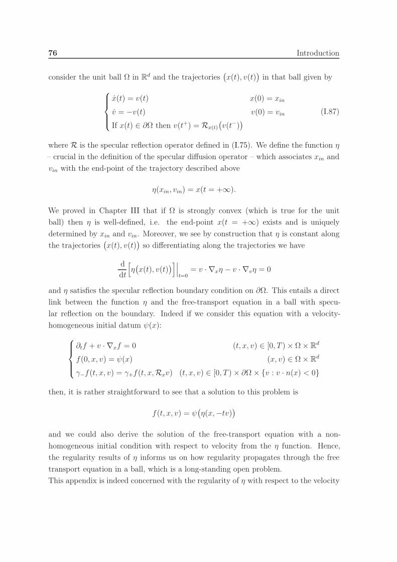
76 Introduction
consider the unit ball Ω in Rd and the trajectories(x(t), v(t)
)in that ball given by
x(t) = v(t) x(0) = xin
v = −v(t) v(0) = vin
If x(t) ∈ ∂Ω then v(t+) = Rx(t)
(v(t−)
)(I.87)
where R is the specular reflection operator defined in (I.75). We define the function η
– crucial in the definition of the specular diffusion operator – which associates xin and
vin with the end-point of the trajectory described above
η(xin, vin) = x(t = +∞).
We proved in Chapter III that if Ω is strongly convex (which is true for the unit
ball) then η is well-defined, i.e. the end-point x(t = +∞) exists and is uniquely
determined by xin and vin. Moreover, we see by construction that η is constant along
the trajectories(x(t), v(t)
)so differentiating along the trajectories we have
d
dt
[η(x(t), v(t)
)]∣∣∣t=0
= v · ∇xη − v · ∇vη = 0
and η satisfies the specular reflection boundary condition on ∂Ω. This entails a direct
link between the function η and the free-transport equation in a ball with specu-
lar reflection on the boundary. Indeed if we consider this equation with a velocity-
homogeneous initial datum ψ(x):
∂tf + v · ∇xf = 0 (t, x, v) ∈ [0, T )× Ω× Rd
f(0, x, v) = ψ(x) (x, v) ∈ Ω× Rd
γ−f(t, x, v) = γ+f(t, x,Rxv) (t, x, v) ∈ [0, T )× ∂Ω × v : v · n(x) < 0
then, it is rather straightforward to see that a solution to this problem is
f(t, x, v) = ψ(η(x,−tv)
)
and we could also derive the solution of the free-transport equation with a non-
homogeneous initial condition with respect to velocity from the η function. Hence,
the regularity results of η informs us on how regularity propagates through the free
transport equation in a ball, which is a long-standing open problem.
This appendix is indeed concerned with the regularity of η with respect to the velocity
I.4 List of works presented in this thesis and perspectives 77
variable. We show that in the unit ball, η has an explicit formulation as a function of
xin, vin and the number k of reflections on the boundary undergone by the trajectory
from (xin, vin), which is always finite when Ω is strongly convex. Through careful
manipulations of the explicit expression and elaborate differential computations, we
are able to show the following regularity results:
Lemma I.4.1. Consider the unit ball Ω. The associated function η defined above
satisfies
‖∇vη(x, v)‖∈ L∞(Ω× Rd) (I.88)
and for all ψ ∈ DT (Ω) defined as
DT (Ω) =ψ ∈ C∞([0, T )× Ω) s.t. ψ(T, ·) = 0 and ∀x ∈ ∂Ω : ∇xψ(t, x) · n(x) = 0
we have
∥∥∥D2v
[ψ(η(x, v)
)]∥∥∥ ∈ LpF (v)(Ω× Rd) (I.89)
for any p < 3 where ‖·‖ is a matrix norm. Moreover,
supv∈Rd
∥∥∥D2v
[ψ(η(x, v)
)]∥∥∥ ∈ L2−δ(Ω) (I.90)
for any δ > 0 and finally, if we write v = rθ with r ∈ R+ and θ ∈ Sd−1 then
supr>0
∣∣∣∆[ψ(η(x, ·)
)](rθ)
∣∣∣ ∈ L∞((0, T );L2(Ω× S
d−1)). (I.91)
Results (I.88), (I.89) and (I.90) come from the appendix of [Ces16] and are tailor-made
in order to prove convergence of the weak formulation of the fractional Vlasov-Fokker-
Planck equation with a well-chosen test function. Although we do not pretend that
these results are optimal, our method of proof fails to ensure the bound (I.90) for
δ = 0 and we have strong doubts that any better regularity could be obtained.
Result (I.91) comes from the appendix of [CH16] and is, once again, custom-made
for the proof of the diffusion limit of the Vlasov-Fokker-Planck equation. Note that,
although we still do not claim optimality, our proof fails to give a result uniformly in
v hence the necessity to take the supremum only with respect to the norm r = |v|. If
we took the supremum in v, the Laplacian would belong to L2−δ(Ω) for any δ > 0 like
the second derivative above.
78 Introduction
Perspectives
There are two naturally continuation of this analysis. The first is to obtain a more
general regularity result of η in the unit ball, such as regularity with respect to the
position variable x and up to the boundary. This regularity issues have been inves-
tigate through energy estimates in [GKTT17] by Y. Guo, C. Kim, D. Tonon and A.
Trescases. Together with A. Trescases, we are currently trying to combine these two
approaches in order to derive optimal regularity in the particular case of the unit ball.
The second natural continuation is to extend the results to more general domains.
The fact is that the explicit formula for η, upon which all our analysis rests, only
holds in a ball and there is a strong possibility that explicit formulae cannot be obtain
in more general domains, especially ones without any particular symmetries. This
is a long-standing open problem, on which we are working. Note that deriving such
results would allow, almost immediately, to derive the specular diffusion equation in
general domains through a very minor modification of the method presented in [Ces16].

Chapter II
Anomalous diffusion limit with an
external electric field
Joint work with Pedro Aceves-Sanchez
Fractional diffusion limit for a fractional Vlasov-Fokker-Planck equation,arXiv:1606.07939, (2016).
Contents
II.1 Introduction . . . . . . . . . . . . . . . . . . . . . . . . . . . 79
II.1.1 The fractional Vlasov-Fokker-Planck equation . . . . . . . . 79
II.1.2 Preliminaries on the Fractional Fokker-Planck operator . . . 81
II.1.3 Main results . . . . . . . . . . . . . . . . . . . . . . . . . . . 83
II.2 Existence of solution . . . . . . . . . . . . . . . . . . . . . . 85
II.3 A priori estimates . . . . . . . . . . . . . . . . . . . . . . . . 90
II.4 Anomalous diffusion limit . . . . . . . . . . . . . . . . . . . 96
II.4.1 The non-critical case: 1/2 < s < 1 . . . . . . . . . . . . . . 97
II.4.2 The critical cases s = 1/2 and s = 1 . . . . . . . . . . . . . 101
II.1 Introduction
II.1.1 The fractional Vlasov-Fokker-Planck equation
In this chapter we investigate the long-time/small mean-free-path asymptotic be-
haviour in the low-field case of the solution of a Vlasov equation with a fractional

80 External electric field
Fokker-Planck operator (VFFP) equation
∂tf + v · ∇xf + E · ∇vf = ∇v · (vf)−(−∆v
)sf in [0,∞)× R
d × Rd, (II.1a)
f(0, x, v) = f in(x, v) in Rd × R
d, (II.1b)
where s ∈ [1/2, 1]. This equation describes the evolution of the density of an ensemble
of particles denoted as f(t, x, v) in phase space, where t ≥ 0, x ∈ Rd and v ∈ Rd
stand for, respectively, time, position and velocity. The operator(−∆
)sdenotes the
fractional Laplacian and is defined by (II.5). Let us recall that, at a microscopic level,
equation (II.1a)-(II.1b) is related to the Langevin equation
dx(t) = v(t) dt,
dv(t) = −v(t) dt+ E dt+ dL2st , (II.2)
where L2st is a Lévy process with generator −
(−∆
)sand (x(t), v(t)) describe the po-
sition and velocity of a single particle (see [JR11] and [Ris96]). Therefore, this models
describes the position and velocity of a particle that is affected by three mechanisms:
a dragging force, an acceleration and a pure jump process.
In the particular case when s = 1 the fractional operator(− ∆
)stakes the form of
a Laplace operator −∆ and (II.1a)-(II.1b) reduces to the usual Vlasov-Fokker-Planck
equation. In this case the Fokker-Planck operator is known to have an equilibrium
distribution function given by a Maxwellian M(v) = C exp (−|v|2) where C > 0
is a normalization constant. The Vlasov-Fokker-Planck equation has been used in
the modeling of many physical phenomena, in particular, for the description of the
evolution of plasmas [Ris96]. However, there are some settings in which particles may
have long jumps and an 2s-stable distribution process is more suitable to describe the
phenomenon, see for instance [SLD+01]. The classical Vlasov-Fokker-Planck equation
for a given external field is related to the Vlasov-Poisson-Fokker-Planck system (VPFP)
in the case in which the electric field is self-consistent. Questions such as existence of
solutions, hydrodynamic limits and long time behaviour for the VPFP system has been
extensively studied by many authors, see for instance [BD95], [Pfa92], and [GNPS05].
In particular, in [EGM10] the low field limit is studied for the VPFP system and a
Drift-Diffusion-Poisson system is obtained in a rigorous manner.
Let us note that, although it is classical in the framework of kinetic theory to consider
a self-consistence electric fields that expresses how particles repulse one another, one
can also, in the VPFP system, consider the case in which particles are attracted by
each other and this model is used in the description of galactic dynamics.

II.1 Introduction 81
In the rest of the chapter we shall need the following notation: The fractional (or
Lévy) Fokker-Planck operator denoted by Ls and defined as
Lsf = ∇v ·(vf)−(−∆v
)sf. (II.3)
In order to investigate the asymptotic behaviour of the system, we introduce the
Knudsen number ε which represent the ratio between the mean-free-path and the
observation length scale. In the case when E = 0 it was observed in [CMT12] that the
time rescaling t′ → ε2s−1t and introducing a factor 1/ε in front of Ls is the appropriate
scaling at which diffusion will be observed in the limit as ε goes to zero. Moreover,
we introduce the factor 1/ε2−2s in front of the force field term E corresponding to
a low-field limit scaling since we shall consider the case 1/2 ≤ s ≤ 1 and thus the
scaling of the collision operator 1/ε is much greater than the scaling of the electric
field 1/ε2−2s. We shall study in this paper the asymptotic behaviour as ε tends to zero
of the solutions of following rescaled VLFP equation
ε2s−1∂tfε + v · ∇xf
ε + ε2s−2E(t, x) · ∇vfε =
1
ε
(∇v · (vf)−
(−∆v
)sf). (II.4)
II.1.2 Preliminaries on the Fractional Fokker-Planck operator
In this chapter we denote by f or F(f) the Fourier transform of f and define it as
f(k) =
∫
Rd
e−ik·xf(x) dx.
There are several equivalent definitions of the fractional Laplacian in the whole domain
(see [Kwa15] or [DPV12]). It can be defined via a Fourier multiplier as
F((
−∆)s(f))(k) = |k|2sF(f)(k).
On the other hand, assuming that f is a rapidly decaying function we can define the
fractional Laplacian in terms of a hypersingular integral as
(−∆v
)s(f)(v) = cd,s P.V.
∫
Rd
f(v)− f(w)
|v − w|d+2sdw (II.5)
where P.V. denotes the Cauchy principal value and the constant cd,s is given by
cd,s =22sΓ
(d+2s2
)
2πd/2|Γ (−s) | , (II.6)

82 External electric field
and Γ(·) denotes the Gamma function. In [DPV12] it is proven that for any d > 1,
cd,s → 0 as s → 1. Thus (II.5) does not make sense if we take s = 1. However, we
have the following result.
Proposition II.1.1. Let d > 1. Then for any f ∈ C∞0 (Rd) we have
lims→1
(−∆
)sf = −∆f.
For an account of the properties of the fractional Laplacian consult [DPV12], [V14],
[Ste70] or [Lan72]. Let us note that due to its dependence on the whole domain,
the fractional Laplacian is a nonlocal operator and it has the scaling property(−
∆v
)s(fλ)(v) = λ2s
(−∆v
)sf(λv), for any λ > 0 where fλ(v) = f(λv). Since it will be
useful later on in our analysis, we also mention that since the fractional Laplacian is
an integro-differential operator it satisfies:
∫ (−∆
)sf dv = 0.
In [BK03] it is proved that the Lévy-Fokker-Planck operator Ls defined by (II.3) has
a unique normalized equilibrium distribution that we shall denote F (which depends
on s). Therefore, the Fourier transformation of F denoted as F and defined as
F (ξ) :=
∫
Rd
e−iξ·vF (v) dv,
satisfies
ξ · ∇ξF + |ξ|2sF = 0.
Thus yielding
F (ξ) = e−|ξ|2s/2s. (II.7)
In the jargon of stochastic analysis, random variables having a characteristic function
of the form (II.7) are called symmetric 2s-stable random variables, consult [App09].
Using the notation of [BJ07] let us note that setting t = 1/2s, x = v, and y = 0, we
obtain the identity F (v) = p(1/2s, v, 0). Thus Lemma 3 of [BJ07] states that there
exists C1 = C1(d, s) > 0 such that
C−11
(1
2s|v|d+2s∧ 1
(2s)d/2s
)≤ F (v) ≤ C1
(1
2s|v|d+2s∧ 1
(2s)d/2s
), (II.8)
II.1 Introduction 83
for all v ∈ Rd, where a∧ b denotes the minimum between a and b. On the other hand,
Lemma 5 of [BJ07] states the existence of a positive constant C2 = C2(d, s) such that
|v|C2
(1
2s|v|d+2+2s∧ (2s)(d+2)/2
)≤∣∣∇vF (v)
∣∣ ≤ C2|v|(
1
2s|v|d+2+2s∧ (2s)(d+2)/2
). (II.9)
II.1.3 Main results
As usually in the framework of fractional Vlasov-Fokker-Planck equations, we use the
following definition of weak solutions:
Definition II.1.1. Consider f in in L2(Rd × Rd) and E ∈(W 1,∞([0, T )× Rd)
)d. We
say that f is a weak solution of (II.1a)-(II.1b) if, for any φ ∈ C∞c ([0, T )× Rd × Rd)
∫∫∫
QT
f(∂tφ+ v · ∇xφ+
(E(t, x)− v
)· ∇vφ−
(−∆
)sφ)dtxv
+
∫∫
Rd×Rd
f in(x, v)φ(0, x, v) dxv = 0
(II.10)
where QT := [0, T )×Rd×R
d. Section 2 of this chapter is devoted to a well-posedness
result for the fractional Vlasov-Fokker-Planck with an external electric field E in the
following sense.
Theorem II.1.2. For f in in L2(Rd × Rd) and E ∈
(W 1,∞([0, T )× R
d))d
there exists
a unique weak solution f of (II.1a)-(II.1b) in the sense of Definition II.1.1 and it
satisfies
f(t, x, v) ≥ 0 on QT , (II.11a)
f ∈ X :=
f ∈ L2(QT ) :
|f(t, x, v)− f(t, x, w)||v − w| d+2s
2
∈ L2(QT × Rd)
. (II.11b)
Remark II.1.3. The assumption E ∈(W 1,∞([0, T )×Rd)
)din Theorem II.1.2 is not
optimal in the sense that we could replace it by E ∈(L∞([0, T ) × Rd)
)dor maybe
it could be replaced by even weaker assumptions on E, however, finding the optimal
regularity of E is out of the scope of this chapter.
The proof of this existence result relies on using the Lax-Milgram theorem for a well
chosen associated problem, in the spirit of the proof in [Deg86] and in [Car98] for
the existence of weak solutions of the Vlasov-Fokker-Planck equation. The proof of
84 External electric field
positivity (II.11a) is given in details as it involves the non-local nature of the fractional
operator and, therefore, differs from the classical proof.
In Section 3, we consider the electric field as a perturbation of the fractional Fokker-
Planck operator and as such we introduce Tε:
Tε(f) := ∇v ·[(v − ε2s−1E(t, x)
)f]−(−∆v
)sf.
We prove existence and uniqueness of a normalized equilibrium Fε for this perturbed
operator in Proposition II.3.1. Then, following the strategy introduced in [ASS17], we
investigate the decay properties of this equilibrium and its convergence to the equilib-
rium of the unperturbed operator, F , as ε goes to 0, in Proposition II.3.2. Finally, we
prove that Tε is dissipative with regards to the quadratic entropy, Proposition II.3.3,
which allows us to establish uniform boundedness results for fε, the solution of the
rescaled equation (II.4)-(II.1b), as well as its macroscopic density ρε =∫fε dv and its
distance to the kernel of Tε we which write rε defined by the expansion fε = ρεFε+εsrε.
In the last section, we turn to the proof of our main result which is the anomalous
advection-diffusion limit of our kinetic model. We follow the method introduced in
[CMT12] which consist in choosing a test function φε(t, x, v) which is solution, for
some ψ ∈ C∞c ([0, T )× Rd) of the auxiliary problem:
εv · ∇xφε − v · ∇vφε = 0 in [0,∞)× Rd × Rd,
φε(t, x, 0) = ψ(t, x) in [0,∞)× Rd,
and show that the weak formulation of our problem, (II.14), with such test functions
converges to the weak formulation of the advection fractional diffusion equation. We
first prove this convergence in the non-critical case, i.e. when 1/2 < s < 1 and then we
turn to the critical cases s = 1/2 and s = 1. The outline of the proof remains the same
in both critical cases but a few differences appear. For s = 1, although the nature of
the collision operator changes noticeably since it becomes local, the only difference in
the proof is a technical one in the study of the dissipative property of the perturbed
operator whereas, in the case s = 1/2, we show that the equilibrium of the perturbed
operator is independent of ε and as such it stays perturbed by the electric field E(t, x)
even in the macroscopic limit. In all cases, our main result reads:
Theorem II.1.4. Let s be in (1/2, 1] and fε be the weak solution of (II.4)-(II.1b)
in the sense of Definition II.1.1 on [0, T ) × Rd × Rd for some T > 0 and with
f in ∈ L2F−1(v)(R
d × Rd) ∩ L1
+(Rd × R
d). Then, fε converges weak-∗ to ρ(t, x)F (v)

II.2 Existence of solution 85
in L∞(0, T ;L2F−1(v)(R
d × Rd)), where ρ is the solution in the distributional sense of
∂tρ+∇ · (Eρ) +(−∆
)sρ = 0 in [0, T )× Rd,
ρ(0, x) = ρin(x) in Rd,(II.12)
where ρin =∫f in dv. In the case s = 1/2 the same anomalous advection-diffusion
limit holds but instead of F (v) the equilibrium distribution of velocity becomes
FE(t, x, v) = F(v −E(t, x)
)(II.13)
The advection fractional-diffusion equation (II.12) describes the evolution of the macro-
scopic density ρ under the effect of a drift, consequence of the kinetic electric field,
and a fractional diffusion phenomenon. The regularity of the solutions of this type
of equations has been studied for instance in [Sil11], [Sil12], and [DI06]. We refer
the interested reader to those articles and references within for more details on this
macroscopic model.
II.2 Existence of solution
We recall that, throughout this paper, for any T > 0 we write QT = [0, T )× Rd × Rd
and C∞c (QT ) the set of smooth function compactly supported in QT . This section
is devoted to the proof of the following result of existence and regularity of weak
solutions:
Theorem II.2.1. Consider f in in L2(Rd × Rd). There exists a unique weak solution
f of (II.1a)-(II.1b) on QT in the sense that for any φ ∈ C∞c (QT ):
∫∫∫
QT
f(∂tφ+ v · ∇xφ+
(E(t, x)− v
)· ∇vφ−
(−∆
)sφ)dtxv
+
∫∫
Rd×Rd
f in(x, v)φ(0, x, v) dxv = 0
(II.14)
and this solution satisfies:
f(t, x, v) ≥ 0 on QT ,
f ∈ X :=
f ∈ L2(QT ) :
|f(t, x, v)− f(t, x, w)||v − w| d+2s
2
∈ L2(QT × Rd)
. (II.15)

86 External electric field
Remark II.2.2. Note that this definition of X is equivalent to saying that it is the
set of functions which are in L2([0, T )× Rd) with respect to time and position and in
Hs(Rd) with respect to velocity.
Proof. We follow the method in [Deg86] and in [Car98] for the proof of existence and
uniqueness of solutions to the linear Vlasov-Fokker-Planck equation. The first part
of the proof consists in solving our linear problem in a variational setting, applying
the well-known Lax-Milgram theorem of functional analysis. We consider the Hilbert
space X provided with the norm
||f ||X =
(||f ||2L2(QT ) + 2c−1
d,s||(−∆)s2 f ||2L2(QT )
) 12
(II.16)
where cd,s is defined in (II.6). We refer the reader to [DPV12] for properties of this
functional space. Let us denote T the transport operator, given by
T f = ∂tf + v · ∇xf −(v − E(t, x)
)· ∇vf.
We define the Hilbert space Y as:
Y =
f ∈ X : T f ∈ X ′
(II.17)
where X ′ is the dual of X . (·, ·)X ,X ′ stands for the dual relation between X and its
dual. Y is provided with the norm:
||f ||2Y = ||f ||2X + ||T f ||2X ′. (II.18)
In order to apply the Lax-Milgram theorem we consider the associated problem
∂tf + e−tv · ∇xf + etE(t, x) · ∇vf + e2st(−∆
)sf + λf = 0 (t, x, v) ∈ QT
f(0, x, v) = f in(x, v) (x, v) ∈ Rd × R
d
(II.19)
which comes formally by deriving (II.1a) for f = e−(λ+d)tf(t, x, e−tv
)and f in(x, v) =
f in(x, e−tv) for some λ ≥ 0. A weak solution of (II.19) is a function f ∈ X such that

II.2 Existence of solution 87
for any φ in C∞c (QT ):
∫∫∫
QT
(− f∂tφ− e−tf v · ∇xφ− etfE(t, x) · ∇vφ+ e2stf
(−∆
)sφ+ λfφ
)dt dx dv
−∫∫
Rd×Rd
f inφ(0, x, v) dx dv = 0.
(II.20)
We first prove existence of a solution in X of equation (II.19) and we will prove after-
wards how this implies existence of a solution of the fractional Vlasov-Fokker-Planck
equation with the electric field E.
We know that C∞c (QT ) is a subspace of X with a continuous injection (see, e.g.
[DPV12]) and we define the prehilbertian norm:
|φ|2C∞c (QT ) = ||φ||2X +
1
2||φ(0, ·, ·)||2L2(Ω×Rd).
Now, we can introduce the bilinear form a : X × C∞c (QT ) → R as:
a(f , φ) =
∫∫∫
QT
(− f∂tφ−e−tf v ·∇xφ−etfE(t, x)·∇vφ+e
2stf(−∆
)sφ+λfφ
)dt dx dv
and the continuous bounded linear operator L on C∞c (QT ) given by:
L(φ) = −∫∫
Rd×Rd
f in(x, v)φ(0, x, v) dx dv.
To find a solution f in X of equation (II.20) is equivalent to finding a solution f in Xof a(f , φ) = L(φ) for any φ ∈ C∞
c (QT ). Since f belongs to X it is easy to check that
a(·, φ) is continuous. To verify the coercivity of a we write:
−∫∫∫
QT
(φ∂tφ+ e−tφv · ∇xφ− etφE(t, x) · ∇vφ
)dt dx dv =
1
2
∫∫
Rd×Rd
|φ(0, x, v)|2 dx dv
and also:∫∫∫
QT
e2stφ(−∆
)sφ dt dx dv =
∫∫∫
QT
e2st|(−∆)s2φ|2 dt dx dv.

88 External electric field
Hence, we see that
a(φ, φ) =
∫∫∫
QT
(λφ2 + e2st|(−∆)
s2φ|2
)dt dx dv +
1
2
∫∫
Ω×Rd
|φ(0, x, v)|2 dt dx dv
which can be bounded from below as a(φ, φ) ≥ min(1, λ)|φ|2C∞c (QT ). Thus, the Lax-
Milgram theorem implies the existence of f in X satisfying (II.20). Now, we want to
show that this yields existence of a solution of (II.14). To that end, we first consider
φ in C∞c (QT ) such that φ(t, x, v) = eλtφ(t, x, e−tv). Equation (II.20) becomes (writing
φ(e−tv) instead of φ(t, x, e−tv))
∫∫∫
QT
eλt(− f∂tφ(e
−tv)− fe−tv · ∇xφ(e−tv) + f e−tv · ∇vφ(e
−tv)
− fE(t, x) · ∇vφ(e−tv) + f
(−∆
)sφ(e−tv)
)dtxv −
∫∫
Rd×Rd
finφ(0, x, v) dxv = 0.
Hence, if we define f(t, x, v) = e(λ+d)tf(t, x, etv) and change the variable v → e−tv, we
recover equation (II.14). It is straightforward to check that f is in X and it satisfies
(II.14) for any φ in C∞c (QT ). Moreover, since f 7→ df −
(−∆
)sf is a linear bounded
operator from X to X ′, the transport term T f is in X ′, hence f ∈ Y and (II.14) is
verified in X ′.
Since the VLFP equation is linear, to show uniqueness it is enough to show that the
unique solution with zero initial data is the null function f ≡ 0. Let f be a solution
of this problem on Y . As before, we define f = e−(λ+d)tf(t, x, e−tv), which satisfies
equation (II.19) with fin null. Since f ∈ Y , we know that f belongs to X and,
moreover, that if we define T as
T f = ∂tf + e−tv · ∇xf + etE(t, x) · ∇vf (II.21)
then T f belongs to X ′. Through integration by parts we have
2(T f , f
)X ′,X
=
∫∫
Rd×Rd
(f)2(T, x, v) dx dv ≥ 0.

II.2 Existence of solution 89
On the other hand, since f satisfies (II.19), T f = −λf −(− ∆
)sf in the sense of
distributions which yields
(T f , f
)X ′,X
= −∫∫∫
QT
(λf 2 + e2st
∣∣(−∆)s2 f∣∣2)dt dx dv ≤ 0. (II.22)
Hence both expression are null, in particular this means that the integral λf 2 is null,
hence f = f ≡ 0 a.e. on QT : the solution is unique. In order to prove the positivity
of the solution consider once again the associated problem (II.19) and its solution f
for some f in ∈ L2(Rd ×Rd) with f in ≥ 0. Next, we define f+ and f− the positive and
negative parts of f given by:
f+(t, x, v) = max(f(t, x, v), 0); f−(t, x, v) = max(−f(t, x, v), 0)
so that f = f+ − f− and we denote by A+ and A− the respective supports of f+ and
f−. Using T defined in (II.21) we have through integration by parts
(T f , f−
)=
∫∫∫
QT
(f−∂t
(f+ − f−
)+ e−tf−v · ∇x
(f+ − f−
)
+ etf−E(t, x) · ∇v
(f+ − f−
))dt dx dv
= −1
2
∫∫
Rd×Rd
(f 2−(T, x, v)− f 2
−(0, x, v))dx dv
+
∫∫∫
QT
(f−∂tf+ + e−tf−v · ∇xf+ + etf−E(t, x) · ∇vf+
)dt dx dv.
By definition of f+ and f− we know that A+ ∩A− = ∅, hence wherever f− is not zero,
both ∂tf+, ∇xf+ and ∇vf+ are naught, and vice-versa. Moreover, we assume f in ≥ 0
which means f−(0, x, v) = 0 so that
(T f , f−
)= −1
2
∫∫
Rd×Rd
f 2−(T, x, v) dx dv ≤ 0.
90 External electric field
Since f is solution of (II.19) we know that T f = −λf −(− ∆
)sf in the sense of
distributions which yields
(T f , f−
)=
∫∫∫
QT
(− λf−
(f+ − f−
)− f−
(−∆
)s(f+ − f−
))dt dx dv
where
∫
Rd
f−(−∆
)s(f+) dv =
∫
Rd
f−(v) cd,s P.V.∫
Rd
f+(v)− f+(w)
|v − w|d+2sdw dv
=
∫
A−
f−(v) cd,s P.V.∫
A+
f+(v)− f+(w)
|v − w|d+2sdw dv
= −cd,s∫
A−
P.V.∫
A+
f−(v)f+(w)
|v − w|d+2sdw dv ≤ 0.
Note that this integral is well defined because f ∈ X . Hence, we have:
(T f , f−
)=
∫∫∫
QT
(λf 2
− − f−(−∆
)sf+ +
∣∣(−∆)s/2f−∣∣2)dtxv ≥ 0.
This proves that(T f , f−
)= 0 which, in particular, means λf 2
− = 0 and concludes the
proof of positivity, and consequently the proof of Theorem II.2.1.
II.3 A priori estimates
Let us consider the operator Tε: a perturbation of the fractional Fokker-Planck oper-
ator with an electric field E(t, x) ∈(W 1,∞([0, T )× Rd)
)ddefined as
Tε(fε) = ∇v ·[(v − ε2s−1E(t, x)
)fε
]−(−∆v
)sfε. (II.23)
We will prove the following:
Proposition II.3.1. For any ε > 0 fixed, there exists a unique positive equilibrium
distribution Fε solution of:
Tε(Fε) = ∇v ·[(v − ε2s−1E(t, x)
)Fε
]−(−∆v
)sFε = 0,
∫
Rd
Fε dv = 1. (II.24)
II.3 A priori estimates 91
Proof. The Fourier transform in velocity of the equilibrium equation (II.24) reads
ξ · ∇ξFε = −(iξ · ε2s−1E(t, x) + |ξ|2s
)Fε,
for which we can compute the explicit solution:
Fε(t, x, ξ) = κe−iε2s−1ξ·E(t,x)−|ξ|2s/2s, (II.25)
where κ is a positive constant which ensures the normalisation of the equilibrium. Now,
although the inverse Fourier transform F−1(Fε)(t, x, v) is not explicit let us note that
Fε can be expressed as a translation of the equilibrium distribution F of the fractional
Fokker-Planck operator:
Fε(t, x, v) = F(v − ε2s−1E(t, x)
). (II.26)
Hence, the positivity and normalization of Fε follows from the properties of F .
Proposition II.3.2. Let Fε be the unique normalized equilibrium distribution of (II.23).
Then there exist positive constants µ, c1, c2 and c3 such that:
(i) c1F ≤ Fε ≤ c2F ,
(ii)
∥∥∥∥∂tFεFε
∥∥∥∥L∞( dv dx dt)
,
∥∥∥∥v · ∇xFεFε
∥∥∥∥L∞( dv dxdt)
≤ ε2s−1µ,
(iii) |Fε − F | ≤ ε2s−1c3F .
for ε > 0 small enough.
Proof. We shall start by proving part (i). Let us assume that L is an arbitrary vector
in Rd such that |L| ≤ 1, then is easy to see that there exists R1 > 0 big enough such
that for all |v| > R1
1
21
d+2s
≤∣∣∣∣1−
|L||v|
∣∣∣∣ ≤∣∣∣∣v
|v| −L
|v|
∣∣∣∣.
Hence, it follows that
1
|v − L|d+2s≤ 2
|v|d+2s,
for all |v| > R1. Thus, using (II.8) we obtain that there exists C > 0 and R > 0 big
enough such that

92 External electric field
F (v − L) ≤ CF (v),
for all |v| > R and all L ∈ Rd with L ≤ 1. Now, let us consider C2 > 0 such that
C2
(min
v∈B(0,R)F (v)
)≥ ‖F‖∞,
where B(0, R) ⊂ Rd, is the ball of radius R centered at the origin. Let us note that
the minimum exists since F is continuous. Thus choosing µ2 = C ∨ C2, where a ∨ bdenotes the maximum between a and b, we obtain
F (v − L) ≤ µ2F (v).
Next, writing w = v + L where L ∈ Rd with |L| ≤ 1 we obtain
F (w) ≤ µ1F (w − L),
Thus, taking µ1 = 1/µ2 we obtain
µ1F (v) ≤ F (v − L),
for all v ∈ Rd and |L| ≤ 1.
On the other hand, for part (ii), let us start by noting that thanks to (II.26), Fεsatisfies the following identities:
∂tFεFε
= −ε2s−1∂tE(t, x) ·∇v F
(v − ε2s−1E(t, x)
)
F(v − ε2s−1E(t, x)
) ,
andv · ∇xFεFε
= −ε2s−1∇xE(t, x)v · ∇v F
(v − ε2s−1E(t, x)
)
F(v − ε2s−1E(t, x)
) .
Hence, thanks to the assumption E ∈(W 1,∞([0, T ) × Rd)
)dwe only need to prove
that there exists a C > 0 such that
|v · ∇v F (v − L)| ≤ CF (v − L), (II.27)
for all v ∈ Rd, and all L ∈ Rd with |L| ≤ 1. This follows via a similar line of reasoning
as in the proof of part (i) around the control (II.9).
Finally we prove part (iii). Since F is smooth by the mean value theorem we obtain

II.3 A priori estimates 93
|Fε(v)− F (v)| = |F (v − ε2s−1E)− F (v)|= ε2s−1|E||∇v F (v − ϑ ε2s−1E)|,
where ϑ ∈ (0, 1). Thus, the result follows thanks to (II.27) and since E ∈(W 1,∞([0, T )×
Rd))d
.
The key ingredient in order to obtain the a priori estimates needed to pass to the limit
in (II.4) is the positivity of the dissipation which we state in the following result.
Proposition II.3.3. Let us consider the operator Tε defined by (II.23). The associated
dissipation, defined bellow, satisfies
Dε(f) := −∫∫
Tε(f)f
Fεdv dx =
∫∫∫ (f(v)
Fε(v)− f(w)
Fε(w)
)2Fε(v)
|v − w|d+2sdw dv dx,
(II.28)
and if we write ρ(t, x) =∫f(t, x, v) dv, then for all f ∈ L2
F−1ε(Rd × R
d) we have
Dε(f) ≥∫(f − ρFε)
2 dx dv
Fε(v). (II.29)
Proof. The Poincaré type inequality (II.29) is a particular case of the so-called Φ-
entropy inequalites introduced in [GI08]. For the sake of completeness we shall give a
sketch of the proof adapted to the case that we need.
We shall first start proving (II.28). Writing Φε = v − ε2s−1E(t, x) and g = f/Fε, and
since Fε satisfies (II.24) we have:
Dε(f) = −∫∫ (
∇v · (ΦεgFε) g −(−∆v
)s(gFε) g
)dv dx
= −∫∫ (
ΦεFε1
2∇v(g
2) +∇v · (ΦεFε)g2 −(−∆v
)s(g)gFε
)dv dx
=
∫∫ (12g2(−∆v
)s(Fε)− g2
(−∆v
)s(Fε) + g
(−∆v
)s(g)Fε
)dv dx
=
∫∫ (g(−∆v
)s(g)− 1
2
(−∆v
)s(g2)
)Fε dv dx.

94 External electric field
Hence, using (II.5) we see that:
∫∫ (g(−∆v
)s(g)− 1
2
(−∆v
)s(g2)
)Fε dv dx
=
∫∫∫ (g(v)
(g(v)− g(w)
)
|v − w|d+2s− 1
2
g2(v)− g2(w)
|v − w|d+2s
)Fε(t, x, v) dw dv dx
=1
2
∫∫∫ (g(v)− g(w)
)2
|v − w|d+2sFε(t, x, v) dw dv dx.
Recall that Fε(t, x, v) = F(v − ε2s−1E(t, x)
), therefore through a simple change of
variable, if we call h(t, x, v) = g(v − ε2s−1E(t, x)
)we have:
Dε(f) =1
2
∫∫∫ (h(t, x, v)− h(t, x, w)
)2
|v − w|d+2sF (v) dw dv dx.
In order to prove the control (II.29) we consider the semigroup associated with(−∆
)s
d
dtPt(h)(v) = −
(−∆
)s(Pt(h)
)(v) (II.30)
with P0(h)(v) = h(v) and we see, using (II.25), that if we introduce the kernel
Kt(v) = F−1(κe−t|ξ|
2s/2s)(v)
where κ is a constant normalizing K1, then we have explicitly Pt(h) = Kt ∗ h. For
s ∈ [0, t] we consider
ψ(s) = Ps(H2)(v) (II.31)
with H = Pt−s(h). We then have for s ∈ [0, t]:
ψ′(s) =d
ds
[Ks ∗
(Kt−s ∗ h
)2]
=( d
dsKs
)∗(Kt−s ∗ h
)2+Ks ∗
d
ds
[(Kt−s ∗ h
)2]
= Ps
(−(−∆
)sH2)+ 2Ps
(H(−∆
)sH)
= Ps
(∫ (H(v)−H(w)
)2
|v − w|d+2sdw
).
Using the integral expression of the convolution and Jensen’s inequality it is straight-
forward to see that(Pt−s(h)(v)−Pt−s(h)(w)
)2 ≤ Pt−s(h(v)−h(w)
)2. Therefore, using

II.3 A priori estimates 95
Fubini’s theorem, we have:
ψ′(s)(v) ≤ Ps
(Pt−s
(∫ (h(v)− h(w)
)2
|v − w|d+2sdw
))= Pt
(∫ (h(v)− h(w)
)2
|v − w|d+2sdw
).
Integrating over s ∈ [0, t] one gets
Pt(h2)(v)−
(Pt(h)(v)
)2≤ tPt
(∫ (h(v)− h(w)
)2
|v − w|d+2sdw
).
Finally, taking t = 1 and evaluating at v = 0 we get:
∫h2(w)F (w) dw−
(∫h(w)F (w) dw
)2
≤∫∫ (
h(v)− h(w))2
|v − w|d+2sF (v) dv dw. (II.32)
Through a simple change of variables, inverse of the one we did earlier, we obtain
∫g2(w)Fε(w) dw−
(∫g(w)Fε(w) dw
)2
≤∫∫ (
g(v)− g(w))2
|v − w|d+2sFε(v) dv dw. (II.33)
Finally, replacing g by f/Fε, since Fε is normalized, we recover (II.29).
Since the operator Tε is negative semidefinite in L2F−1ε(Rd) it is natural to look for
bounds of the quadratic entropy associated to solutions fε of (II.4). We gather the
appropriate a priori estimates that we shall need to pass to the limit in (II.4) in the
following Proposition.
Proposition II.3.4. Let the assumptions of Theorem II.1.4 be satisfied and let fε be
the solution of (II.4). We introduce the residue rε through the macro-micro decompo-
sition fε = ρεFε + εsrε. Then, uniformly in ε ∈ (0, 1), we have:
(i) (fε) is bounded in L∞([0, T );L2F−1(v)(R
d × Rd)) and in L∞([0, T );L1(Rd × Rd)),
(ii) (ρε) is bounded in L∞([0, T );L2(Rd)),
(iii) (rε) is bounded in L2([0, T );L2F−1(v)(R
d × Rd)).
Proof. Multiplying (II.4) by fε/Fε, integrations by parts yield

96 External electric field
ε2s−1
2
d
dt
∫∫
Rd×Rd
f 2ε
Fεdv dx+
ε2s−1
2
∫∫
Rd×Rd
f 2ε
Fε
∂tFεFε
dv dx
− 1
2
∫∫
Rd×Rd
f 2ε
Fε
v · ∇xFεF 2ε
dv dx+1
εDε(f
ε) = 0.
Thus, thanks to Proposition II.3.2, part (i) and (ii), and (II.29) we obtain
ε2s
2
d
dt
∫∫
Rd×Rd
f 2ε
Fεdv dx+
∫∫
Rd×Rd
(fε − ρεFε)2
Fεdv dx ≤ ε2sµ
∫∫
Rd×Rd
f 2ε
Fεdv dx. (II.34)
Whence, part (i) follows by Gronwall’s lemma and the fact that the weights 1/F and
1/Fε are equivalent uniformly in ε which follows from Proposition II.3.2, part (i). On
the other hand, part (ii) follows thanks to the inequality
ρε ≤(∫
f 2ε
Fεdv
)1/2
,
which is an immediate consequence of Cauchy-Schwarz and the fact∫Fε dv = 1.
Finally, part (iii) follows from (II.48) after integrating with respect to t over (0, T )
and thanks to Proposition II.3.2 part (ii).
II.4 Anomalous diffusion limit
We shall follow the method introduced in [CMT12]. Let us start by introducing the
following auxiliary problem: for ψ ∈ C∞c ([0, T )×Rd), define φε the unique solution of
εv · ∇xφε − v · ∇vφε = 0 in [0,∞)× Rd × R
d,
φε(t, x, 0) = ψ(t, x) in [0,∞)× Rd(II.35)
The function φε can be obtained readily via the method of characteristics and can be
expressed in an explicit manner as follows:
φε(t, x, v) = ψ(t, x+ εv). (II.36)
Next, since φε is in C∞c (QT ) we can use it as a test function in (II.14) and we obtain
II.4 Anomalous diffusion limit 97
∫∫∫
QT
fε
(ε2s−1 ∂tφε + v · ∇xφε −
1
ε(v − ε2s−1E) · ∇vφε −
1
ε
(−∆v
)sφε
)dv dx dt
+ ε2s−1
∫∫
Rd×Rd
f in(x, v)φε(0, x, v) dv dx = 0 . (II.37)
Let us note the following
(−∆v
)sφε(t, x, v) = ε2s
(−∆
)sψ(t, x+ εv), (II.38)
∇vφε(t, x, v) = ε∇ψ(t, x+ εv), (II.39)
which follows after a simple computation using the definition (II.5) of the fractional
Laplacian. Thus using the auxiliary equation (II.35) and plugging (II.38) into (II.37)
yields
∫ ∞
0
∫∫fε
(∂tψ(t, x+ εv) + E · ∇xψ(t, x+ εv)−
(−∆
)sψ(t, x+ εv)
)dv dx dt
+
∫∫f in(x, v)ψ(0, x+ εv) dv dx = 0 .
(II.40)
II.4.1 The non-critical case: 1/2 < s < 1
In order to pass to the limit in this weak formulation, we introduce the following two
results.
Lemma II.4.1. Let (fε) be the sequence of solutions of (II.4), and ρ be the limit of
(ρε) which exists thanks to Proposition II.3.4 part (ii), then
fε(t, x, v) ρ(t, x)F (v) weakly in L∞([0, T );L2F−1(v)(R
d × Rd))
Proof. This lemma follows directly from Proposition II.3.4. Since fε is uniformly
bounded, it converges weakly in L∞([0, T );L2F−1(v)(R
d×Rd)). From the bounds on Fεestablished in Proposition II.3.2 and the boundedness of ρε in L∞([0, T );L2(Rd)) we
see that ρε(t, x)Fε(v) converges to ρ(t, x)F (v) weakly in L∞([0, T );L2F−1(v)(R
d × Rd))
where ρ is the weak limit of ρε. Finally, since the residue rε is bounded, it follows
from the micro-macro decomposition fε = ρεFε + εsrε that the limit of fε is the same
as the limit of ρεFε.

98 External electric field
Lemma II.4.2. For all test functions ψ in C∞c ([0,∞)× Rd) we have:
limε→0
∫∫∫
QT
f ε(t, x, v)ψ(t, x+ εv) dt dx dv =
∫∫
[0,T )×Rd
ρ(t, x)ψ(t, x) dx dt. (II.41)
Moreover, if E(t, x) ∈(W 1,∞([0, T )×R
d))d
then for all Ψ ∈ C∞c ([0,∞)×R
d;Rd) the
following convergence holds:
limε→0
∫∫∫
QT
f ε(t, x, v)E(t, x) ·Ψ(t, x+ εv) dt dx dv =
∫∫
[0,T )×Rd
ρ(t, x)E(t, x) ·Ψ(t, x) dx dt.
(II.42)
Proof. We will give a detailed proof of the convergence in (II.42), the convergence in
(II.41) follows as a consequence of (II.42) by taking ψ(t, x+εv) = E(t, x) ·Ψ(t, x+εv),
with a smooth E, and Lemma II.4.1. For (II.42), we write:
∫∫∫
QT
fεE(t, x) ·Ψ(t, x+ εv) dv dx dt =
∫∫
[0,T )×Rd
ρ(t, x)E(t, x) ·Ψ(t, x) dx dt
+
∫∫∫
QT
(fε − ρ(t, x)F (v)
)E(t, x) ·Ψ(t, x) dv dx dt
+
∫∫∫
QT
fεE(t, x) ·(Ψ(t, x+ εv)−Ψ(t, x)
)dv dx dt. (II.43)
The second term in the right hand side of (II.43) converges to zero since fε converges
to ρF weakly in L∞([0, T );L2F−1(v)(R
d × Rd)) thanks to Lemma II.4.1. For the third
term on the right hand side of (II.43) thanks to Cauchy-Schwarz and Hölder we obtain
∣∣∣∣∫∫∫
QT
fεE(t, x) · (Ψ(t, x+ εv)−Ψ(t, x)) dv dx dt
∣∣∣∣
≤∫ T
0
( ∫∫
Rd×Rd
f 2ε
Fdv dx
)1/2( ∫∫
Rd×Rd
[E(t, x) · (Ψ(t, x+ εv)−Ψ(t, x))
]2F dv dx
)1/2
dt
≤ ‖fε‖L∞([0,T );L2F−1(v)
(Rd×Rd))
×∫ T
0
( ∫∫
Rd×Rd
[E(t, x) · (Ψ(t, x+ εv)−Ψ(t, x))]2F dv dx
)1/2
dt. (II.44)

II.4 Anomalous diffusion limit 99
Next, let R be an arbitrary positive real number and let us consider the following
splitting
∫∫
Rd×Rd
[E · (Ψ(t, x+ εv)−Ψ(t, x))
]2F (v) dv dx
=
∫
Rd
∫
|v|≤R
[E · (Ψ(t, x+ εv)−Ψ(t, x))
]2F (v) dv dx
+
∫
Rd
∫
|v|>R
[E · (Ψ(t, x+ εv)−Ψ(t, x))
]2F (v) dv dx. (II.45)
We will use the regularity of Ψ to bound the integral on |v| < R. To that end, let us
consider the εR neighborhood of the support of Ψ denoted as Ω(εR) which consists
of the union of all the balls of radius εR having as center a point in suppΨ. Next,
let Λ denote the diameter of suppΨ defined as the maximum over all the distances
between two points in suppΨ. Then it is clear that Ω(εR) ⊆ B(x0;Λ + εR) where
B(x0;Λ + εR) denotes the ball with center at x0 and radius Λ + εR and x0 is any
arbitrary fix point in suppΨ. Then for the integral over |v| < R we have the following
∫
Rd
∫
|v|≤R
[E · (Ψ(t, x+ εv)−Ψ(t, x))]2F (v) dv dx
≤ ‖F‖L∞(Rd)
∫
Rd
∫
|v|≤R
( d∑
j=1
|Ej |∣∣εv · ∇xΨj(t, x+ θjεv)
∣∣)2
dv dx
≤ 2ε2‖F‖L∞(Rd)
∫
Rd
∫
|v|≤R
|v|2( d∑
j=1
|Ej|2∣∣∇xΨj(t, x+ θjεv)
∣∣2)dv dx
≤ 2ε2‖F‖L∞(Rd)‖E‖2W 1,∞([0,T )×Rd)‖∇xΨ‖L∞(Rd)
∫
|v|≤R
∫
B(x0,δ+εR)
|v|2 dx dv
≤ ε2C2(Λ+ εR)dRd+2, (II.46)
where C2 is a constant depending on ‖E‖2W 1,∞([0,T )×Rd), ‖F‖L∞(Rd) and ‖D2xφ‖L∞(Rd)
but not on ε, and θj ∈ (0, 1) for j = 1, . . . , d is such that Ψj(t, x + εv) − Ψj(t, x) =
εv · ∇xΨj(t, x+ θjεv). For the integral on |v| > R we use the decay of the equilibrium
100 External electric field
F (v) to derive the following upper bound:
∫
Rd
∫
|v|>R
[E · (Ψ(t, x+ εv)−Ψ(t, x))
]2F (v) dv dx
≤ ‖E‖2W 1,∞([0,T )×Rd)
∫
|v|>R
(∫
Rd
(2|Ψ(t, x+ εv)|2 + 2|Ψ(t, x)|2
)dx
)F (v) dv
≤ 4‖E‖2W 1,∞([0,T )×Rd)
∫
Rd
|Ψ(t, x)|2 dx∫
|v|>R
F (v) dv
≤ C
∫
|v|>R
F (v) dv.
Thanks to Proposition II.3.1, for any η > 0 we can choose R > 0 big enough such that
∣∣∣∣F (v)−ϑ
|v|d+2s
∣∣∣∣ ≤η
|v|d+2s, for all |v| ≥ R.
Thus choosing η = ϑ we have the following estimate:
∫
|v|>R
F (v) dv ≤∫
|v|>R
∣∣∣∣F (v)−ϑ
|v|d+2s
∣∣∣∣ dv +∫
|v|>R
ϑ
|v|d+2sdv
≤ 2
∫
|v|>R
ϑ
|v|d+2sdv
≤ C
R2s.
From which we conclude∫
Rd
∫
|v|>R
[E · (Ψ(t, x+ εv)−Ψ(t, x))
]2F (v) dv dx ≤ C2
R2s. (II.47)
Next let us note that for any δ > 0 we can choose R > 0 such that C2/R2s < δ/2 for
all R > R and then choose ε > 0 so that ε2C1(Λ+ εR)dRd+2 < δ/2. And thus deduce
that for ε small enough we have
ε2C1(Λ+ εR)dRd+2 +C2
R2s< δ.
II.4 Anomalous diffusion limit 101
Therefore, plugging (II.46) and (II.47) into (II.44) and using Proposition II.3.4, part
(i), we obtain that there exists a fixed C > 0 such that
∣∣∣∣∫∫∫
QT
fεE · (Ψ(t, x+ εv)−Ψ(t, x)) dv dx dt
∣∣∣∣
≤ C
(ε2C1(Λ+ εR)dRd+2 +
C2
R2s
)
≤ Cδ,
for any δ > 0, hence concluding that the third term on the right hand side of (II.43)
goes to zero as ε→ 0.
Using Lemma II.4.2 we can now take the limit in (II.40) and conclude that ρ satisfies
∫∫
[0,T )×Rd
ρ(∂tφ+ E · ∇xφ−
(−∆x
)sφ)dx dt +
∫
Rd
ρin(x)φ(0, x) dx = 0,
for all φ ∈ C∞c ([0, T )× Rd). Thus concluding the proof of Theorem II.1.4.
II.4.2 The critical cases s = 1/2 and s = 1
In the critical case s = 1 we recover the classical Fokker-Planck operator which means,
in particular, as mentioned in the Introduction, that its equilibrium is a Maxwellian
M(v) = C exp (−|v|2) instead of the heavy-tail distribution F . We can still consider
the perturbed operator Tε of Proposition II.3.1 and its equilibrium will also be a
translation of the unperturbed one:
Fε(t, x, v) = Ce−|v−εE(t,x)|2
and since the decay of the Maxwellian is much faster than the decay of the heavy-tail
distributions, Proposition II.3.2 holds. The dissipative properties of the Fokker-Planck
operator are well known, see e.g. [CH16] [GNPS05] or [BG08], and it is straightforward
to check the boundedness results of Proposition II.3.4. Hence, Lemma II.4.1 holds and
we can take the limit in the weak formulation (II.40) to prove that Theorem II.1.4 holds
in the case s = 1.

102 External electric field
In the critical case s = 1/2, the perturbed operator Tε of (II.23) and its equilibrium
Fε (II.26) lose their dependence with respect to ε:
Tε(fε) = TE(fε) := ∇v ·[(v − E(t, x)
)fε
]−(−∆v
)sfε,
Fε(t, x, v) = FE(t, x, v) := F(v −E(t, x)
)
where F is the normalized equilibrium of L1/2. In particular, the equilibrium FE will
remain unchanged in the limit as ε goes to 0 and Proposition II.3.2 will hold with
s = 1/2 which, in particular, means that the bounds in (ii) and (iii) do not go to zero.
The operator is still dissipative since the dependence on ε does not matter in the proof
of Proposition II.3.3, hence we still have (II.33) and multiplying (II.4) by fε/FE and
integrating by parts yields:
ε
2
d
dt
∫∫
Rd×Rd
f 2ε
FEdv dx+
∫∫
Rd×Rd
(fε − ρεFE)2
FEdv dx ≤ εµ
∫∫
Rd×Rd
f 2ε
FEdv dx. (II.48)
Since E is in(W 1,∞([0, T )× Rd)
)d, if fε(t, ·, ·) is in L2
FE(t,x,v)(Rd × Rd) and bounded
independently of time, then it is also in L2F (v)(R
d×Rd). As a consequence, from (II.48)
we still have the uniform in ε boundedness of fε, ρε =∫fε dv and the residue rε in
L∞([0, T );L2F (v)(R
d × Rd)) as stated in Proposition II.3.4. This yields the following
modified version of Lemma 1:
Lemma II.4.3. Let s = 1/2, (fε) be the sequence of solutions of (II.4), and ρ be the
limit of (ρε) which exists thanks to Proposition II.3.4 part (ii), then
fε(t, x, v)⋆ ρ(t, x)FE(t, x, v) in L∞([0, T );L2
F−1(v)(Rd × R
d)).
Finally, for the proof of convergence of the weak formulation (II.40), i.e. the proof of
Lemma II.4.2, we proceed essentially the same way. The only slight difference is that
in order to control the third term of (II.43) we will use Cauchy-Schwarz as in (II.44)
but we multiply and divide by F (v)1/2 instead of the natural equilibrium FE . The rest
of the proof remains the same and we can then take the limit in the weak formulation,
which concludes the proof of Theorem II.1.4 with s = 1/2.

Chapter III
Anomalous diffusion limit in spatially
bounded domains
Contents
III.1 Introduction . . . . . . . . . . . . . . . . . . . . . . . . . . . 104
III.1.1 Preliminaries on the fractional Fokker-Planck operator . . . 109
III.1.2 Main Results . . . . . . . . . . . . . . . . . . . . . . . . . . 111
III.2 A priori estimates . . . . . . . . . . . . . . . . . . . . . . . . 117
III.3 Absorption in a smooth convex domain . . . . . . . . . . . 120
III.3.1 Auxiliary problem . . . . . . . . . . . . . . . . . . . . . . . 121
III.3.2 Macroscopic Limit . . . . . . . . . . . . . . . . . . . . . . . 122
III.4 Specular Reflection in a smooth strongly convex domain . 123
III.4.1 Auxiliary problem . . . . . . . . . . . . . . . . . . . . . . . 124
III.4.1.1 Construction of η . . . . . . . . . . . . . . . . . . 125
III.4.1.2 φε solution of the auxiliary problem . . . . . . . . 128
III.4.2 Macroscopic limit . . . . . . . . . . . . . . . . . . . . . . . . 129
III.4.2.1 Lemma III.4.1 in a half-space . . . . . . . . . . . . 130
III.4.2.2 Lemma III.4.1 in a ball . . . . . . . . . . . . . . . 135
III.5 Well posedness of the specular diffusion equation . . . . . 137
III.5.1 Properties and estimates of the specular diffusion operator . 137
III.5.1.1 (−∆)sSR
on the half-space . . . . . . . . . . . . . . 137
III.5.1.2 (−∆)sSR
on a ball . . . . . . . . . . . . . . . . . . . 141
104 Anomalous diffusion limit in spatially bounded domains
III.5.1.3 The Hilbert space HsSR(Ω) . . . . . . . . . . . . . . 143
III.5.2 Existence and uniqueness of a weak solution for the macro-
scopic equation . . . . . . . . . . . . . . . . . . . . . . . . . 144
III.5.3 Identifying the macroscopic density as the unique weak solu-
tion . . . . . . . . . . . . . . . . . . . . . . . . . . . . . . . 146
III.1 Introduction
Because of the non-local nature of fractional diffusion, it is not clear how it should in-
teract with a boundary. In an effort to understand this interaction, we present in this
chapter the derivation of fractional diffusion equations on spatially bounded domain
from kinetic equations with a fractional Fokker-Planck collision operator. This setting
is particularly relevant due the fact that, in those kinetic equations, the non-local
collision operator acts solely on the velocities of the particles which are unbounded,
hence the interaction between the non-local phenomena in position and the spatial
boundary will only arise as we look at the anomalous diffusion limit.
We investigate the long time/small mean-free-path asymptotic behaviour of the solu-
tion of the fractional Vlasov-Fokker-Planck (VFP) equation:
∂tf + v · ∇xf = ∇v · (vf)− (−∆v)sf in R
+ × Ω× Rd, (III.1a)
f(0, x, v) = fin(x, v) in Ω× Rd, (III.1b)
for s ∈ (0, 1) on a smooth convex domain Ω. We introduce the oriented set:
Σ± = (x, v) ∈ Σ;±n(x) · v > 0 with Σ = ∂Ω× Rd (III.2)
where n(x) is the outgoing normal vector and we denote by γf the trace of f on
R+ × ∂Ω×Rd. The boundary conditions then take the form of a balance between the
values of the traces of f on these oriented sets γ±f := 1Σ±γf . We will consider two
types of conditions introduced by J. C. Maxwell in the appendix of [Max79] in 1879:
• The absorption boundary condition : for all (x, v) ∈ Σ−
γ−f(t, x, v) = 0 (III.3)
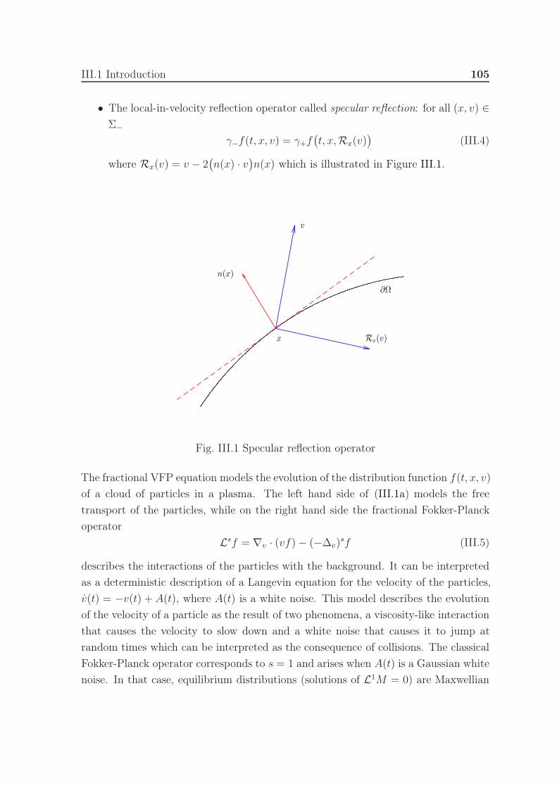
III.1 Introduction 105
• The local-in-velocity reflection operator called specular reflection: for all (x, v) ∈Σ−
γ−f(t, x, v) = γ+f(t, x,Rx(v)
)(III.4)
where Rx(v) = v − 2(n(x) · v
)n(x) which is illustrated in Figure III.1.
v
Rx(v)x
n(x)
∂Ω
Fig. III.1 Specular reflection operator
The fractional VFP equation models the evolution of the distribution function f(t, x, v)
of a cloud of particles in a plasma. The left hand side of (III.1a) models the free
transport of the particles, while on the right hand side the fractional Fokker-Planck
operator
Lsf = ∇v · (vf)− (−∆v)sf (III.5)
describes the interactions of the particles with the background. It can be interpreted
as a deterministic description of a Langevin equation for the velocity of the particles,
v(t) = −v(t) + A(t), where A(t) is a white noise. This model describes the evolution
of the velocity of a particle as the result of two phenomena, a viscosity-like interaction
that causes the velocity to slow down and a white noise that causes it to jump at
random times which can be interpreted as the consequence of collisions. The classical
Fokker-Planck operator corresponds to s = 1 and arises when A(t) is a Gaussian white
noise. In that case, equilibrium distributions (solutions of L1M = 0) are Maxwellian

106 Anomalous diffusion limit in spatially bounded domains
(or Gaussian) velocity distributions M = C exp(−|v|2/2). However, some experimen-
tal measurements of particles and heat fluxes in confined plasma point to non-local
features and non-Gaussian distribution functions. The introduction of Lévy statistic
in the velocity equation (replacing the Gaussian white noise by Lévy white noise in the
Langevin equation) can be seen as an attempt at taking into account these non-local
effects in plasma turbulence.
In order to study the long time/small mean free path asymptotic behaviour of the
solutions of the fractional VFP equation, we introduce the Knudsen number ε which
represents the ratio of the mean-free-path to the macroscopic length scale, or equiva-
lently the ratio of the mean time between two collisions to the macroscopic time scale.
We use this ε to rescale the time variable as
t′ = ε2s−1t. (III.6)
Moreover, we also introduce 1/ε as a factor of the fractional Fokker-Planck operator to
model the mean-free-path growing smaller as a consequence of the number of collisions
per unit of time increasing. Hence, we consider the following scaling of (III.1a)-(III.1b):
ε2s−1∂tfε + v · ∇xf
ε =1
εLs(f ε)
in R+ × Ω× R
d, (III.7a)
f ε(0, x, v) = fin(x, v) in Ω× Rd. (III.7b)
and investigate the behaviour of the solution f ε when ε goes to 0.
In the non-fractional framework, the diffusion limits under parabolic scaling of the
Vlasov-Fokker-Planck equations, which is exactly (III.7a) with s = 1, have been estab-
lished on the whole space in 2000 by Poupaud-Soler in [PS00] for a small enough time
interval. They actually studied the more complicated Vlasov-Poisson-Fokker-Planck
system but it is easy to see that their results imply, for the VFP equation, that the
solution f ε converges, as ε goes to 0, to ρ(t, x)M(v) where M is the Maxwellian equilib-
rium of the Fokker-Planck operator and ρ is the limit of the density ρε =∫f ε dv and
satisfies a Heat-equation. Their results were then extended (still in the Poisson case)
in 2005 by Goudon [Gou05] to a global in time convergence in dimension 2 with bounds
on the entropy and energy of the initial data as to ensure that they don’t develop sin-
gularities in the limit system, and later in 2010 by El Ghani-Masmousi [EGM10] who
proved the global in time convergence in higher dimensions with similar initial bounds.

III.1 Introduction 107
In the fractional framework, Biler-Karch [BK03] and Gentil-Imbert [GI08] investigate
the long-time behaviour of Lévy-Fokker-Planck equations
∂tf = div (f∇φ) + I[f]
(III.8)
where I is the infinitesimal generator of a Lévy process. This family of operators
includes the fractional Fokker-Planck operator since the fractional Laplacian of order s
is the generator of a particular 2s-stable Lévy process whose characteristic exponent is
|ξ|2s. Biler-Karch prove convergence of the solution of (III.8) to the unique normalised
equilibrium of the Lévy-Fokker-Planck operator, later improved by Gentil-Imbert to
exponential convergence in a weighted L2 space where the weight is prescribed by the
equilibrium. Their proofs use entropy production methods and a modified logarithmic
Sobolev inequality which we will use later on to establish a priori estimates on the
solutions of the fractional VFP equation in a similar weighted L2 space. In [GM06]
and references within, Guan-Ma give a description of this equilibrium and proofs that
it is, in particular, heavy-tailed, as stated below in Proposition III.1.1.
This characterisation of the equilibrium of the fractional Fokker-Planck operator and
the entropy production method allowed the author with A.Mellet and K. Trivisa to
establish in [CMT12] the anomalous diffusion limit of the fractional VFP equation.
More precisely, we proved the following result:
Theorem (Theorem 1.2 in [CMT12]). Assume that f0 ∈ L2F−1(Rd × Rd) where F (v)
is the normalised heavy-tailed equilibrium of the fractional Fokker-Planck operator.
Then, up to a subsequence, the solution f ε of the rescaled fractional VFP equation
on the whole space (III.7a)-(III.7b) converges weakly in L∞(0, T ;L2F−1(Rd × Rd)), as
ε → 0 to ρ(t, x)F (v) where ρ(t, x) solves
∂tρ+ (−∆x)sρ = 0 in (0,∞)× R
d (III.9a)
ρ(0, x) = ρ0(x) in Rd (III.9b)
with ρ0(x) =∫f0(x, v) dv.
We can see how this result compares to the aforementioned diffusion limit of the
classical Vlasov-Fokker-Planck. However, the method used in [CMT12] to derive this
asymptotic behaviour is quite different from what is done is the non-fractional case,
and rests upon the particular structure of the fractional VFP equation. Indeed, and
this will be essential for the rest of this paper, if we consider the Fourier transform
108 Anomalous diffusion limit in spatially bounded domains
of (III.1a) in x and v (respective Fourier variables k and ξ) on Rd × Rd we get the
following PDE:
∂tf(t, k, ξ) + (k − ξ)∇ξf(t, k, ξ) = −|ξ|2sf(t, k, ξ). (III.10)
This PDE is scalar-hyperbolic so if we follow well-chosen characteristic lines, it be-
comes an ODE which can be solved explicitly. The main idea of [CMT12] is to trans-
pose these characteristic lines in a non-Fourier setting in order to derive fractional
diffusion. The method presented in the present work consists in adapting these same
characteristic lines to a bounded domain in order to handle the interaction with a
boundary.
Kinetic equations on bounded domains, because of their obvious physical relevance,
have always received a lot of attention. There have been many works concerning exis-
tence of global weak solutions on bounded domains with absorbing-type or reflection-
type boundary conditions. We would like to mention the work of Carrillo [Car98] on
the VPFP system, as well as the work of Mellet-Vasseur [MV07] for the VFP equa-
tion coupled to compressible Navier-Stokes via drag force, because their techniques
could be applied to the fractional VFP equation with some adaptations to handle the
non-local property of the diffusion operator and we will indeed follow the line of reason-
ing of [Car98] to prove well-posedness of the specular diffusion equation in section III.5.
Hydrodynamical and diffusion limits in bounded domains have also been the subject
of many works. For instance, in 1987, Degond-Mas-Gallic [DMG87] established the
first rigorous diffusion limit for the (classical) VFP equation in 1 dimension on a
bounded domain. This result has been improved many times (cf. references within
[WLL15b]), and in 2015 Wu-Lin-Lui proved in [WLL15b] that the diffusion limit of
a VPFP system for multiple species charged particles with reflection boundary condi-
tions is a Poisson-Nernst-Planck system with homogeneous Neumann boundary condi-
tions. Other examples of macroscopic limits are the work Masmoudi-Saint-Raymond
who, in 2003, showed in [MSR03] that the Boltzmann equation with Maxwell boundary
conditions converges to the Stokes-Fourier system with Navier boundary conditions,
or, more recently, the work of Jiang-Levermore-Masmoudi who established in [JLM09]
the acoustic limit for DiPerna-Lions solutions and recovered impermeable boundaries
for the acoustic system.
III.1 Introduction 109
Before stating our main results, let us present properly the fractional Laplacian and
give some well-known properties of this operator and the associated fractional Fokker-
Planck operator.
III.1.1 Preliminaries on the fractional Fokker-Planck operator
The fractional Laplacian can be defined as a pseudo-differential operator of symbol
|ξ|2s which can be written in Fourier transform as:
F[(
−∆)sf(ξ)
]= |ξ|2sF [f ](ξ). (III.11)
Much like the Laplace operator is the infinitesimal generator of a Brownian motion,
the fractional Laplacian is the generator of a Lévy process. More precisely, it is the
generator of a Lévy process Vt whose transition density ρ(t, y − x) relative to the
Lebesgue measure is given in Fourier by:
∫
Rd
eiv·ξρ(t, v) dv = e−t|ξ|2s
.
The fractional Laplacian can also be written as a singular integral, which will be most
useful in the PDE framework:
(−∆
)sf(v) = cs,dP.V.
∫
Rd
f(v)− f(w)
|v − w|d+2sdw (III.12)
where cs,d is a constant depending on s and the dimension d given by:
cd,s =
(∫
Rd
1− cos(ζ1)
|ζ |d+2sdζ
)−1
. (III.13)
The properties of this operator have been studied in 2007 by Silvestre in [Sil07] and
more recently by DiNezza-Palatucci-Valdinoci in [DPV12] where they focus on the
link between(−∆
)sand the fractional Sobolev spaces Hs(Rd).
The interaction between the non-locality of the fractional Laplacian and the boundary
of a domain raises a lot of questions. In 2003, Bogdan-Burdzy-Chen introduced in
[BBC03] the notion of reflected 2s-stable processes, which are the restriction of a 2s-
stable process, such as Vt defined above, to a open set Ω in Rd. In particular, they
define the killed process, constructed by adding a coffin state ∂ to Rd and defining Wt,
110 Anomalous diffusion limit in spatially bounded domains
the killed process associated with Vt, as:
Wt(ω) =
∣∣∣∣∣Vt(ω) for t ≤ tΩ(ω)
∂ for t > tΩ(ω)
where tΩ = inft > 0 : Vt /∈ Ω is the first exit time. The Dirichlet form of this process
on L2(Ω, dx) is (C,FΩ) defined as:
FΩ =
f ∈ L2(Rd) :
∫∫
Rd×Rd
(f(x)− f(y)
)2
|x− y|d+2sdx dy <∞ and f = 0 q.e. on R
d \ Ω
C(f, g) = 1
2cd,s
∫∫
Ω×Ω
(f(x)− f(y)
)(g(x)− g(y)
)
|x− y|d+2sdx dy +
∫
Ω
f(x)g(x)κΩ(x) dx
where q.e. means quasi everywhere and κΩ is the density of the killing measure of Wt
given by:
κΩ(x) = cd,s
∫
Rd\Ω
1
|x− y|d+2sdy.
They also define more general reflected processes by extending the lifetime of the
process beyond tΩ. The killed process has a direct link with the PDE approach to
fractional Laplacian on bounded domain. Indeed, in 2014, Felsinger-Kassmann-Voigt
considered in [FKV13], the Dirichlet problem for non-local operators which, in case of
the fractional Laplacian, reads:
(−∆
)sf = u in Ω
f = g on Rd \ Ω. (III.14)
They introduced the Hilbert space HΩ
(Rd; 1
|x−y|d+2s
), which is exactly the space FΩ
defined above, provided with the norm ||f ||L2(Rd) + C(f, f). They wrote a variational
formulation of the Dirichel problem (III.14) in that Hilbert space and proved existence
and uniqueness of solutions. Note that their results actually include a large family of
non-local operators, we stated it here for the fractional Laplacian since it is the subject
of this paper, but their work goes far beyond. For regularity results on the solutions of
the homogeneous dirichlet problem with fractional Laplacian inside the domain and up
to the boundary, we refer the reader to Grubb [Gru13] and Ros-Oton-Serra [ROS14].
The fractional Fokker-Planck operator Ls has been introduced as a generalization
of the classical Fokker-Planck operator for general Lévy stable processes in 2000 by

III.1 Introduction 111
Yanovsky-Chechkin-Schertzer-Tur [YCST00] and the following year it was derived
from the wider class of non-linear Langevin-type equation driven by a Lévy stable noise
by Schertzer-Larchevêque-Duan-Yanovsky-Lovejoy in [SLD+01]. In the present paper,
the most crucial property of the fractional Fokker-Planck operator will be the fact
that its thermodynamical equilibrium is a Lévy stable distribution i.e. a heavy-tailed
distribution, instead of the Maxwellian distribution that arise in the non-fractional
setting. The explicit solution in Fourier transform of the equation LsF = 0 yields the
following result
Proposition III.1.1. For s ∈ (0, 1) and ν > 0, there exists a unique normalized
equilibrium distribution function F (v), solution of
Ls(F ) = ν∇v · (vF )− (−∆v)sF = 0,
∫
Rd
F (v) dv = 1. (III.15)
Furthermore, F (v) > 0 for all v, and F is a heavy-tailed distribution function satisfying
F (v) ∼ C
|v|d+2sas |v| → ∞.
For a more detailed presentation of the equilibrium of Ls we refer the reader to [ASC16]
and references within.
III.1.2 Main Results
Throughout this paper, for any T > 0 we write QT = [0, T )× Ω×Rd and Σ = ∂Ω×Rd
as mentioned in (V.2). Also, we will write Lp(Σ±) the Lebesgue space associated with
the norm:
‖γ±f‖Lp(Σ±)=
(∫∫
Σ±
|γ±f |p(n(x) · v
)dσ(x) dv
)1/p
(III.16)
As usually in the framework of fractional Vlasov-Fokker-Planck equations we use the
following definitions of weak solutions
Definition III.1.1. We say that f is a weak solution of the fractional VFP equation
with Dirichlet type boundary conditions (III.1a)-(III.1b)-(III.3) on [0, T ) if
f(t, x, v) ≥ 0 ∀(t, x, v) ∈ [0, T )× Ω× Rd
f ∈ L2t,xH
sv(QT ) =
f ∈ L2(QT ),
f(t, x, v)− f(t, x, w)
|v − w| d+2s2
∈ L2(QT × Rd)
(III.17)

112 Anomalous diffusion limit in spatially bounded domains
satisfies
γ±f ∈ L1(0, T ;L1(Σ±)
), and γ−f = 0 (III.18)
and (III.1a) holds in the sense that for any φ such that
φ ∈ C∞(QT ) φ(T, ·, ·) = 0
γ+φ(t, x, v) = 0 ∀(t, x, v) ∈ [0, T )× Σ+
(III.19)
we have: ∫∫∫
QT
f(∂tφ+ v · ∇xφ− v · ∇vφ−
(−∆v
)sφ)dt dx dv
−∫∫
Ω×Rd
fin(x, v)φ(0, x, v) dx dv = 0.
(III.20)
In the case of specular reflection, it is well known that reflective boundaries are often
responsible for a loss of regularity of the traces of f . Hence, we define the following
notion of weak solutions:
Definition III.1.2. We say that f is a weak solution of (III.1a)-(III.1b)-(III.4) on
[0, T ) if
f(t, x, v) ≥ 0 ∀(t, x, v) ∈ [0, T ]× Ω× Rd
f ∈ L2t,xH
sv(QT ) =
f ∈ L2(QT ),
f(t, x, v)− f(t, x, w)
|v − w| d+2s2
∈ L2(QT × Rd)
(III.21)
and (III.1a) holds in the sense that for any φ such that:
φ ∈ C∞(QT ) φ(T, ·, ·) = 0
γ+φ(t, x, v) = γ−φ(t, x,Rx(v)
)∀(t, x, v) ∈ [0, T )× Σ+
(III.22)
we have:∫∫∫
(0,T )×Ω×Rd
f(∂tφ+ v · ∇xφ− v · ∇vφ−
(−∆v
)sφ)dt dx dv
−∫∫
Ω×Rd
fin(x, v)φ(0, x, v) dx dv = 0.
(III.23)
The existence and uniqueness of such weak solutions that satisfy appropriate esti-
mates can be established through an adaptation of the methods of Carrillo in [Car98]
III.1 Introduction 113
or Mellet-Vasseur [MV07] in order to handle the non-local property of the diffusion
operator. We do not dwell on this issue since it is not the focus of this paper.
In the first part of this paper, section III.2, we establish a priori estimates on the weak
solutions, in both the absorption and the specular reflection case, using the dissipative
property of the fractional Fokker-Planck operator. We then use those estimates to
prove convergence of the weak solution of the rescaled fractional VFP equation:
Proposition III.1.2. Let fin be in L2F−1(v)(Ω × Rd) and s be in (0, 1). The weak
solution f ε of the rescaled fractional VFP equation (III.7a)-(III.7b) with absorption
(III.3) or specular reflections (III.4) on the boundary satisfies
f ε(t, x, v) ρ(t, x)F (v) weakly in L∞(0, T ;L2
F−1(v)(Ω× Rd))
(III.24)
where ρ(t, x) is the limit of the macroscopic densities ρε =∫Rd f
ε dv.
In sections 3 and 4, we establish the anomalous diffusion limits, i.e. we identify the
limit ρ as solution of a diffusion equation. The main idea of these proofs is to take ad-
vantage of the aforementioned scalar-hyperbolic structure of the fractional VFP equa-
tion in Fourier space (III.10). To that end, we introduce an auxiliary problem whose
purpose is to construct, from any test function ψ(t, x), a function φε(t, x, v) which
will be constant along the characteristic lines of the fractional VFP equation modi-
fied to take into account the boundary conditions, and such that limεց0 φε(t, x, v) =
ψ(t, x). For the absorption boundary condition, the auxiliary problem reads for
ψ ∈ D([0, T )× Ω):
εv · ∇xφε − v · ∇vφ
ε = 0 ∀(t, x, v) ∈ R+ × Ω× R
d, (III.25a)
φε(t, x, 0) = ψ(t, x) ∀(t, x) ∈ R+ × Ω, (III.25b)
γ+φε(t, x, v) = 0 ∀(t, x, v) ∈ R
+ × Σ+. (III.25c)
We construct a solution of this problem and use it as a test function in the weak
formulation of (III.7a)-(III.7b)-(III.3). We then show that we can take the limit in
the weak formulation to prove:
Theorem III.1.3. Assume that fin is in L2F−1(v)(Ω × Rd) and s is in (0, 1). Then
the solution f ε of (III.7a)-(III.7b)-(III.3), converges weakly in the sense of Proposition
III.1.2 to ρ(t, x)F (v) where the extension of ρ(t, x) by 0 outside of Ω is a weak solution

114 Anomalous diffusion limit in spatially bounded domains
of
∂tρ+(−∆
)sρ = 0 (t, x) ∈ [0, T )× Ω (III.26a)
ρ(x, 0) = ρin(x) x ∈ Ω (III.26b)
ρ(t, x) = 0 t ∈ [0, T ), x ∈ Rd \ Ω (III.26c)
where ρin(x) =∫fin dv, in the sense that for all ψ ∈ D([0, T )×Rd) compactly supported
in Ω:∫∫
(0,T )×Rd
ρ(t, x)(∂tψ(t, x)−
(−∆
)sψ(t, x)
)dt dx+
∫
Rd
ρin(x)ψ(0, x) dx = 0. (III.27)
In this macroscopic equation, the extension by 0 of the function ρ can be interpreted as
an extension of (III.3), the homogeneous Dirichlet boundary condition in the kinetic
equation, to the whole complementary of the domain Ω as a consequence of the non-
local nature of the fractional Laplacian operator.
For the specular reflection boundary condition, if we want follow the characteristic
lines as they reflect on the boundary, we need to reduce (when s ≥ 1/2) the set of test
functions to DT (Ω) defined as:
DT (Ω) =ψ ∈ C∞([0, T )× Ω) s.t. ψ(T, ·) = 0 and ∀x ∈ ∂Ω : ∇xψ(t, x) · n(x) = 0
.
(III.28)
The auxiliary problem reads for ψ ∈ DT :
εv · ∇xφε − v · ∇vφ
ε = 0 ∀(t, x, v) ∈ R+ × Ω× R
d, (III.29a)
φε(t, x, 0) = ψ(t, x) ∀(t, x) ∈ R+ × Ω, (III.29b)
γ+φε(t, x, v) = γ−φ
ε(t, x,Rx(v)
)∀(t, x, v) ∈ R
+ × Σ+. (III.29c)
In order to construct a solution of this auxiliary problem we study geodesic trajectories
in a Hamiltonian billiard. These trajectories are given by, parametrised with s ∈ [0,∞)
x(s) = εv(s) x(0) = xin ∈ Ω,
v(s) = −v(s) v(0) = vin ∈ Rd,
If x(s) ∈ ∂Ω then v(s+) = Rx(s)(v(s−)),
(III.30)
as illustrated in Figure III.2 for example when Ω is a ball. We construct a function
η : Ω×Rd 7→ Ω that will be constant along those trajectories, defined as η(xin, vin) =
lims→∞ x(s) which obviously, strongly depends on the geometry of the domain and
III.1 Introduction 115
we will show that it is well defined when Ω is a half-space or a ball. This η function
allows us to find a solution of the auxiliary problem:
Proposition III.1.4. If Ω is either a half-space or smooth and strongly convex, then
there exists a function η : Ω× Rd → Ω such that
φε(t, x, v) = ψ(t, η(x, εv)
)(III.31)
is a solution of the auxiliary problem (III.29a)-(III.29b)-(III.29c).
Although the regularity of this η function is rather simple to study in the half-space,
it is much harder to understand in the ball and we will devote Appendix A to this
investigation. In fact, it is strongly linked with the free transport equation. Indeed, if
we consider the following free transport equation in a ball with specular reflection on
the boundary and a homogeneous-in-velocity initial condition:
∂tf + v · ∇xf = 0 (t, x, v) ∈ [0, T )× Ω× Rd
f(0, x, v) = ψ(x) (x, v) ∈ Ω× Rd
γ−f(t, x, v) = γ+f(t, x,Rxv) (t, x, v) ∈ [0, T )× ∂Ω× v : v · n(x) < 0
then, using (III.29a)-(III.29b)-(III.29c) and Proposition III.1.4 we can show that a
solution of this problem is
f(t, x, v) = ψ(η(x,−tv)
).
As a consequence, the regularity properties of η we establish in Appendix A can
also be interpreted as a propagation of regularity with respect to the velocity for the
previous free transport equation. We are then able to establish the following anomalous
diffusion limit.
Theorem III.1.5. Let Ω be either a half-space or a ball in Rd and assume that finis in L2
F−1(v)(Ω × Rd) and s is in (0, 1). Then the solution f ε of (III.7a)-(III.7b)-
(III.3), converges weakly in the sense of Proposition III.1.2 to ρ(t, x)F (v) where ρ(t, x)
satisfies, for any ψ ∈ DT (Ω):
∫∫
(0,T )×Ω
ρ(t, x)(∂tψ(t, x)− (−∆)s
SRψ(t, x)
)dt dx+
∫
Ω
ρin(x)ψ(0, x) dx = 0. (III.32)
116 Anomalous diffusion limit in spatially bounded domains
where ρin(x) =∫fin dv and (−∆)s
SRis defined as:
(−∆)sSRψ(x) = cd,sP.V.
∫
Rd
ψ(x)− ψ(η(x, w)
)
|w|d+2sdw (III.33)
This new operator, which we call specular diffusion operator, can be seen as a modified
version of the fractional Laplacian where the particles can jump from a position x to
a position y in Ω not only through a straight line but also through trajectories that
are specularly reflected when they hit the boundary, and the probability of this jump
is 1/|w|d+2s where |w| is the length of the trajectory. Note that when Ω is Rd, by
definition we have η(x, w) = x + w so that (−∆)sSR
coincides with the full fractional
Laplacian(−∆
)son Rd.
Theorem III.1.5 can also be proved when Ω is a strip x = (x′, xd) ∈ Rd : −1 < xd < 1
or a cube using arguments from the half-space case in order to handle locally the inter-
action with the boundary, and from the ball case to handle the multitude of reflections
a trajectory in a strip or a cube may undergo in a finite time. Moreover, in order to
extend this theorem to general smooth and strongly convex domains, one only needs to
prove that the trajectories described by η in that domain satisfy appropriate controls,
similar to the ones we state in Lemma III.4.2 in the case of the ball which we prove
in Appendix A. The rest of the proof would remain the same.
Finally, in the last section of this paper, we focus on the macroscopic equation (III.57)
which we name specular diffusion equation. First, we establish properties of the spec-
ular diffusion operator (−∆)sSR
. Namely, in the half-space we show that it can be
written as a kernel operator with a symmetric kernel:
(−∆)sSRψ(x) = P.V.
∫
Ω
(ψ(x)− ψ(y)
)KΩ(x, y) dy with KΩ(x, y) = KΩ(y, x).
(III.34)
and such that the kernel is 2s-singular. Then, in both the half-space and the ball,
we show that the operator is symmetric and admits a integration by parts formula.
From this formula we derive a scalar product and defined the associated Hilbert space
HsSR(Ω) in the spirit of the fractional Sobolev spaces in their relation with the fractional
Laplacian operators as is presented for instance in [DPV12]. We conclude this paper
by studying the specular diffusion equation in this setting:
Theorem III.1.6. Let Ω be a half-space or a ball in Rd, uin be in L2((0, T )×Ω) and
s be in (0, 1). For any T > 0, there exists a unique weak solution u ∈ L2(0, T ;HsSR(Ω))

III.2 A priori estimates 117
of
∂tu+ (−∆)sSRu = 0 (t, x) ∈ [0, T )× Ω (III.35a)
u(0, x) = uin(x) x ∈ Ω (III.35b)
in the sense that for any ψ ∈ C∞([0, T )× Ω), u satisfies if Ω is a half-space:
∫∫
(0,T )×Ω
u∂tψ dt dx−∫
Ω
uin(x)ψ(0, x) dx
− 1
2
∫∫∫
(0,T )×Ω×Ω
(u(t, x)− u(t, y)
)(ψ(t, x)− ψ(t, y)
)K(x, y) dt dx dy = 0.
(III.36)
and if Ω is the unit ball
∫∫
(0,T )×Ω
u∂tψ dt dx−∫
Ω
uin(x)ψ(0, x) dx
− 1
2
∫∫∫
(0,T )×Ω×Rd
(u(t, x)− u
(t, η(x, v)
))(ψ(t, x)− ψ
(t, η(x, v)
)) dt dx dv|v|d+2s
= 0.
(III.37)
Moreover, if Ω is a half-space or a ball, then the macroscopic density ρ who satisfies
(III.32) for all ψ ∈ DT (Ω) is the unique weak solution of (III.35a)-(III.35b).
This theorem highlights the fact that the interaction with the boundary in (III.35a)-
(III.35b) is contained in the definition of the diffusion operator (−∆)sSR
since we don’t
need to add a boundary condition in order to have well-posedness.
Here again, although we only look at the half-space and the ball, other geometries can
be handled by our method such as a strip or a cube for example. Furthermore, the
only obstacle to considering more general domains lies in understanding the function η
is those domains in order to establish the symmetry of the specular diffusion operator
and estimates on its singularity.
III.2 A priori estimates
In order to study the asymptotic behaviour of the weak solution of (III.7a)-(III.7b)
with (III.3) or (III.4) boundary condition, we need a priori estimates. Those estimates
will rely on the following dissipation property of the fraction Fokker-Planck operator
Ls

118 Anomalous diffusion limit in spatially bounded domains
Proposition III.2.1. For all f smooth enough, if we define the dissipation as:
Ds(f) := −∫
Rd
Ls(f) fF
dv (III.38)
then there exists θ > 0 such that
Ds(f) =
∫∫
Rd×Rd
(f(v)− f(w)
)2
|v − w|d+2s
dv dw
F (v)≥ θ
∫
Rd
∣∣f(v)− ρF (v)∣∣2 dv
F (v)(III.39)
where ρ =∫Rd f(v) dv. Note, in particular, that Ds(f) ≥ 0.
Proof. We introduce the notation g = f/F (v) and notice by expending the divergence
and integrating by parts that:
∫
Rd
∇v · (vFg)g dv =1
2
∫
Rd
∇v · (vF )g2 dv.
We recall that F satisfies Ls(F ) = 0, which means ∇v · (vF ) = (−∆)s(F ). By
symmetry of the fractional Laplacian and the previous remark we have:
Ds(f) = −∫
Rd
(∇v · (vgF )g − (−∆)s(gF )g
)dv
= −∫
Rd
(∇v · (vF )g2/2− (−∆)s(gF )g
)dv
= −∫
Rd
((−∆)s(F )g2/2− (−∆)s(gF )g
)dv
=
∫
Rd
(− 1
2F (−∆)s(g2) + Fg(−∆)s(g)
)dv.
Inputting the definition (III.12) of the fractional Laplacian we get:
Ds(f) = cs
∫
Rd
P.V.
∫
Rd
−1
2[g(v)2 − g(w)2] + g(v)2 − g(w)g(v)
F (v)
|v − w|d+2sdw dv
=cs2
∫∫
Rd×Rd
F (v)[g(v)− g(w)]2
|v − w|d+2sdv dw.
=cs2
∫∫
Rd×Rd
(f(v)
F (v)− f(w)
F (w)
)2F (v)
|v − w|d+2sdv dw.

III.2 A priori estimates 119
Since v and w play the same role in the integral, we can write
Ds(f) =cs4
∫∫
Rd×Rd
[(f(v)
F (v)− f(w)
F (w)
)2
F (v) +
(f(v)
F (v)− f(w)
F (w)
)2
F (w)
]dv dw
|v − w|d+2s.
Expending the integrand and grouping the terms adequately, it is not difficult to show
that:
Ds(f) =
∫∫
Rd×Rd
(f(v)− f(w)
)2
|v − w|d+2s
dv dw
F (v). (III.40)
Finally, the second inequality in (III.39) comes from the modified logarithmic Sobolev
inequality of Gentil-Imbert (Theorem 3 in [GI08]) which we can use here because F (v)
is the infinitely divisible law associated with the Lévy measure 1/|v|d+2s. We refer the
interested reader to [ASC16] for a proof of this functional inequality in the fractional
Laplacian case.
The dissipation property of Ls allows us to prove the following:
Proposition III.1.2. Let fin be in L2F−1(v)(Ω × Rd) and s be in (0, 1). The weak
solution f ε of the rescaled fractional VFP equation (III.7a)-(III.7b) with absorption
(III.3) or specular reflections (III.4) on the boundary satisfies
f ε(t, x, v) ρ(t, x)F (v) weakly in L∞(0, T ;L2
F−1(v)(Ω× Rd))
(III.24)
where ρ(t, x) is the limit of the macroscopic densities ρε =∫Rd f
ε dv.
Proof. Multiplying (III.7a) by f ε/F (v) and integrating over x and v one gets, after
integrations by parts, for the absorption boundary condition:
ε2s−1 ddt
∫∫
Ω×Rd
(f ε)2 dx dvF (v)
+
∫∫
Σ+
|γ+f ε|2|n(x) · v|dσ(x) dv
F (v)+
1
ε
∫
Ω
Ds(f ε) dx = 0
and in the specular reflections case:
ε2s−1 ddt
∫∫
Ω×Rd
(f ε)2 dx dvF (v)
+1
ε
∫
Ω
Ds(f ε) dx = 0.
120 Anomalous diffusion limit in spatially bounded domains
In both cases, since the dissipation in non-negative, we see that d
dt‖f ε‖L2
F−1(v)(Ω×Rd)≤ 0
so f ε(t, ·, ·) is bounded in L2F−1(v)(Ω× R
d). Moreover, we have
∫∫
(0,T )×Ω
Ds(f ε) dt dx ≤ ε2s(‖fin‖L2
F−1(v)(Ω×Rd)−‖f ε(T, x, v)‖L2
F−1(v)(Ω×Rd)
)−→ε→0
0
and furthermore, by definition of ρε, we see that
ρε ≤(∫
Rd
(f ε)2 dv
F (v)
)1/2(∫∫
Rd
F (v) dv
)1/2
= ‖f ε‖L2F−1(v)
(Rd)
so that ρε is also bounded in L∞(0, T ;L2(Ω)). The boundedness of f ε in L∞(0, T ;L2
F−1(v)(Ω×Rd))
gives us the existence of a weak limit f . Since the dissipation goes to 0, (III.39)
implies that the limit is in the kernel of the fractional Fokker-Planck operator, i.e.
there exists a function ρ such that f(t, x, v) = ρ(t, x)F (v). And finally, the bounded-
ness of ρε gives us existence of a weak limit ρ and by uniqueness of the limit ρ = ρ,
which concludes the proof.
III.3 Absorption in a smooth convex domain
We focus in this section on the absorption boundary condition (III.3) and show how
we can easily adapt the method developed in [CMT12] for the anomalous diffusion
limit of the fractional Vlasov-Fokker-Planck equation to this bounded domain case.
According to Definition III.1.1, if fε is a weak solution of the rescaled equation (III.7a)-
(III.7b) with absorption (III.3) on the boundary then for all φ satisfying (III.19) we
have∫∫∫
QT
f ε(ε2s−1∂tφ− ε−1
(−∆v
)sφ)dt dx dv (III.41a)
+
∫∫∫
QT
f ε(v · ∇xφ− ε−1v · ∇vφ
)dt dx dv (III.41b)
+ ε2s−1
∫∫
Ω×Rd
fin(x, v)φ(0, x, v) dx dv = 0. (III.41c)
III.3 Absorption in a smooth convex domain 121
We recognize, in (III.41b), the characteristic lines of (III.10). In order to take advan-
tage of the scalar-hyperbolic structure of (III.10) we want to consider test functions
which are constant along those lines. This is the purpose of the auxiliary problem.
III.3.1 Auxiliary problem
In the absorption case, it is rather simple to adapt the auxiliary problem introduced
in [CMT12] to the domain Ω. For any ψ ∈ D([0, T )× Ω) we introduce the auxiliary
problem:
εv · ∇xφε − v · ∇vφ
ε = 0 ∀(t, x, v) ∈ R+ × Ω× R
d, (III.25a)
φε(t, x, 0) = ψ(t, x) ∀(t, x) ∈ R+ × Ω, (III.25b)
γ+φε(t, x, v) = 0 ∀(t, x, v) ∈ R
+ × Σ+. (III.25c)
Since the boundary condition (III.25c) is immediately compatible with the assumption
of compactly support in Ω for the test function ψ, the construction of the solution φεis rather straightforward:
Proposition III.3.1. For any ψ ∈ D([0, T )× Ω), φε defined as:
φε(t, x, v) = ψ(t, x+ εv)
where ψ is the extension of ψ by 0 outside Ω, is a solution of (III.25a)-(III.25b)-
(III.25c).
Proof. The proof is almost immediate. For (III.25a) we write:
εv · ∇xφε − v · ∇vφ
ε = εv · ∇x[ψ(t, x+ εv)]− v · ∇v[ψ(t, x+ εv)]
= εv · ∇ψ(t, x+ εv)− εv · ∇ψ(t, x+ εv) = 0.
Moreover, the definition of φε ensures (III.25b) and, thanks to the compact support
of ψ in Ω we also see that φε(t, x, v) = 0 for any (x, v) ∈ Σ+ since it means that
x+ εv /∈ Ω.

122 Anomalous diffusion limit in spatially bounded domains
For such a φε we see that:
(−∆v
)sφε(t, x, v) = cd,sP.V.
∫
Rd
φε(t, x, v)− φε(t, x, w)
|v − w|d+2sdw
= cd,sP.V.
∫
Rd
ψ(t, x+ εv)− ψ(t, x+ εw)
|v − w|d+2sdw
= cd,sP.V.
∫
Rd
ψ(t, x+ εv)− ψ(t, w)
ε−d−2s|x+ εv − w|d+2sε−d dw
= ε2s(−∆
)sψ(t, x+ εv)
(III.43)
so that the weak formulation (III.41a)-(III.41b)-(III.41c) becomes
∫∫∫
QT
f ε(∂tψ −
(−∆
)sψ(t, x+ εv)
)dt dx dv +
∫∫
Ω×Rd
fin(x, v)ψ(0, x+ εv
)dx dv = 0.
(III.44)
III.3.2 Macroscopic Limit
In Section III.2 we proved that f ε converges weakly in L∞(0, T ;L2
F−1(v)(Ω × Rd)).
Hence, in order to pass to the limit in the weak formulation (III.44) we need to show
that
∂tψ(t, x+ εv)−(−∆
)sψ(t, x+ εv) −→
ε→0∂tψ(t, x)−
(−∆
)sψ(t, x) (III.45)
at least strongly in L∞(0, T ;L2
F (v)(Ω × Rd)). The proof of this convergence is rather
similar to its equivalent in the unbounded case presented in [CMT12]. As a conse-
quence we will not give any unnecessary details and instead we briefly recall the main
arguments. First, we note that the continuity of ψ readily implies the convergence of
the second term in (III.44):
∫∫
Ω×Rd
fin(x, v)ψ(0, x+ εv
)dx dv −→
ε→0
∫
Ω
ρin(x)ψ(0, x) dx.
Secondly, the strong convergence of (III.45) follows from the fact that if ψ is in
D([0, T )× Ω) then
∂tψ ∈ D([0, T )× Ω) and(−∆
)sψ ∈ D([0, T )× R
d) ∩ L2([0, T )× Rd)

III.4 Specular Reflection in a smooth strongly convex domain 123
because the pseudo-differential operator(− ∆
)scan be defined as an operator from
the Schwartz space to L2(Rd), see e.g. Proposition 3.3 in [DPV12]. As a consequence,
it is straightforward to use dominated convergence on both terms and prove the strong
convergence of (III.45) in L∞(0, T ;L2
F (v)(Ω× Rd)), noticing that
∫F (v) dv = 1.
Hence, we can take the limit in the weak formulation and find that ρ satisfies:
∫∫
(0,T )×Ω
ρ(t, x)(∂tψ(t, x)−
(−∆
)sψ(t, x)
)dt dx+
∫
Ω
ρin(x)ψ(0, x) dx = 0. (III.46)
Since ρ is the limit of ρε it is only defined on Ω. If we extend it by 0 on the comple-
mentary Rd \ Ω, then we can integrate over Rd instead of Ω and that concludes the
proof of Theorem III.1.3.
III.4 Specular Reflection in a smooth strongly convex
domain
We now turn to the more challenging case of the specular reflection boundary con-
dition (III.4). From Definition III.1.2 we know that if fε is a weak solution of
fractional Vlasov-Fokker-Planck equation with specular reflection on the boundary
(III.7a)-(III.7b)-(III.4) then for any φ satisfying
φ ∈ C∞(QT ) φ(T, ·, ·) = 0
γ+φ(t, x, v) = γ−φ(t, x,Rx(v)
)∀(t, x, v) ∈ [0, T )× Σ+
(III.22)
we have, analogously to the absorption case:
∫∫∫
QT
f ε(ε2s−1∂tφ− ε−1
(−∆v
)sφ)dt dx dv (III.41a)
+
∫∫∫
QT
f ε(v · ∇xφ− ε−1v · ∇vφ
)dt dx dv (III.41b)
+ ε2s−1
∫∫
Ω×Rd
fin(x, v)φ(0, x, v) dx dv = 0. (III.41c)
Once again, we would like to take advantage of the scalar-hyperbolic structure of
(III.10) in order to define a sub-class of test function φ that will allow us to identify

124 Anomalous diffusion limit in spatially bounded domains
the anomalous diffusion limit of this equation. This is the purpose of the following
auxiliary problem.
III.4.1 Auxiliary problem
For a smooth function ψ, we define φε as the solution of
εv · ∇xφε − v · ∇vφ
ε = 0 ∀(t, x, v) ∈ R+ × Ω× R
d, (III.29a)
φε(t, x, 0) = ψ(t, x) ∀(t, x) ∈ R+ × Ω, (III.29b)
γ+φε(t, x, v) = γ−φ
ε(t, x,Rx(v)
)∀(t, x, v) ∈ R
+ × Σ+. (III.29c)
with Rx(v) = v − 2(n(x) · v
)n(x) for x in ∂Ω.
Because of the specular reflection boundary condition (III.29c), it is much more chal-
lenging to construct a solution φε of this problem than it was in the absorption case.
In fact, we will see later on that if we want to have enough regularity estimates on φε in
order to take the limit in the weak formulation of the fractional Vlasov-Fokker-Planck
equation, we will need an additional assumption on the initial condition ψ. Setting
aside these considerations for the moment, let us show how we can construct φε from
smooth function ψ through the definition of a function η : Ω×Rd 7→ Ω in the following
sense:
Proposition III.1.4. If Ω is either a half-space or smooth and strongly convex, then
there exists a function η : Ω× Rd → Ω such that
φε(t, x, v) = ψ(t, η(x, εv)
)(III.48)
is a solution of the auxiliary problem (III.29a)-(III.29b)-(III.29c).
Proof. The proof will consist of two steps. First we construct an appropriate η by iden-
tifying the characteristic lines underlying the hyperbolic problem (III.29a)-(III.29c),
and then we check that φε defined as above is indeed solution of the auxiliary problem.
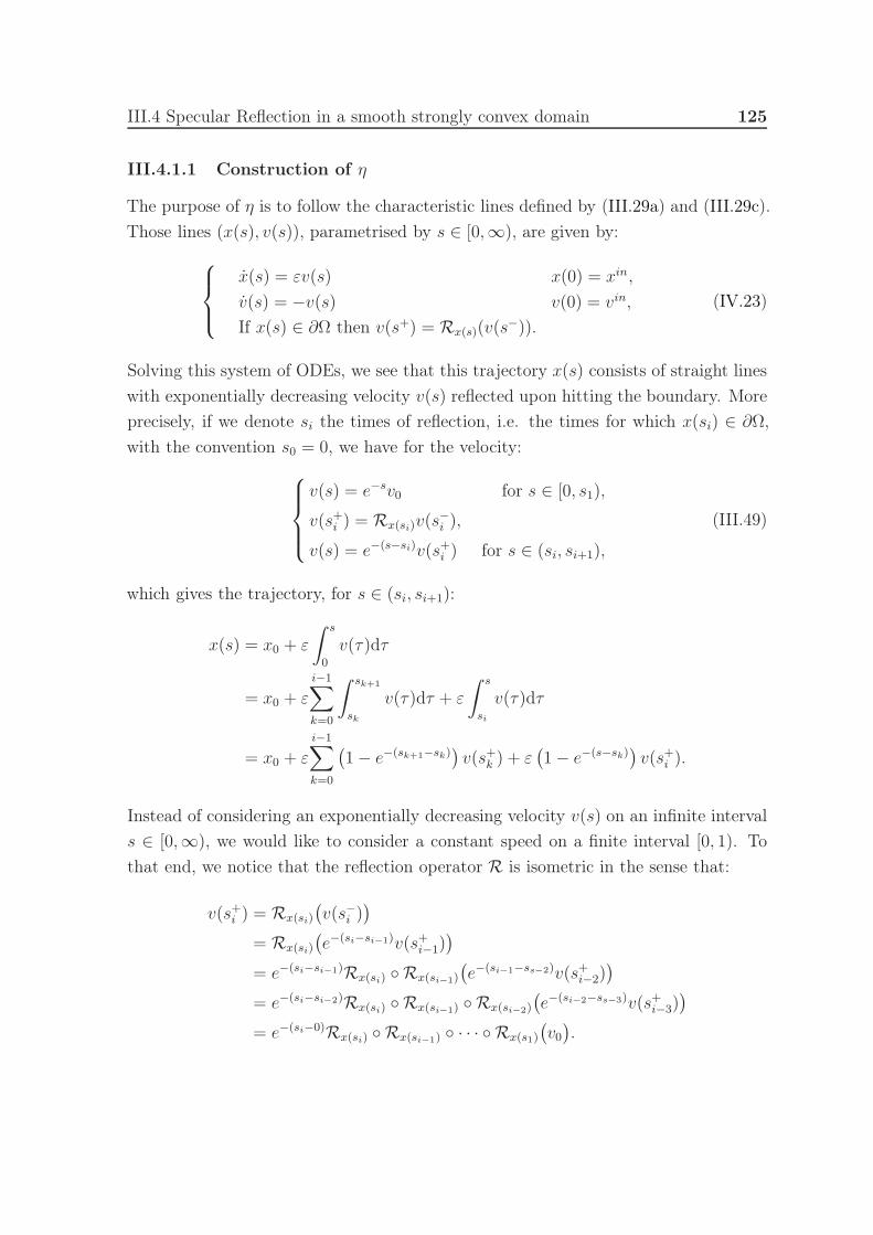
III.4 Specular Reflection in a smooth strongly convex domain 125
III.4.1.1 Construction of η
The purpose of η is to follow the characteristic lines defined by (III.29a) and (III.29c).
Those lines (x(s), v(s)), parametrised by s ∈ [0,∞), are given by:
x(s) = εv(s) x(0) = xin,
v(s) = −v(s) v(0) = vin,
If x(s) ∈ ∂Ω then v(s+) = Rx(s)(v(s−)).
(IV.23)
Solving this system of ODEs, we see that this trajectory x(s) consists of straight lines
with exponentially decreasing velocity v(s) reflected upon hitting the boundary. More
precisely, if we denote si the times of reflection, i.e. the times for which x(si) ∈ ∂Ω,
with the convention s0 = 0, we have for the velocity:
v(s) = e−sv0 for s ∈ [0, s1),
v(s+i ) = Rx(si)v(s−i ),
v(s) = e−(s−si)v(s+i ) for s ∈ (si, si+1),
(III.49)
which gives the trajectory, for s ∈ (si, si+1):
x(s) = x0 + ε
∫ s
0
v(τ)dτ
= x0 + ε
i−1∑
k=0
∫ sk+1
sk
v(τ)dτ + ε
∫ s
si
v(τ)dτ
= x0 + ε
i−1∑
k=0
(1− e−(sk+1−sk)
)v(s+k ) + ε
(1− e−(s−sk)
)v(s+i ).
Instead of considering an exponentially decreasing velocity v(s) on an infinite interval
s ∈ [0,∞), we would like to consider a constant speed on a finite interval [0, 1). To
that end, we notice that the reflection operator R is isometric in the sense that:
v(s+i ) = Rx(si)
(v(s−i )
)
= Rx(si)
(e−(si−si−1)v(s+i−1)
)
= e−(si−si−1)Rx(si) Rx(si−1)
(e−(si−1−ss−2)v(s+i−2)
)
= e−(si−si−2)Rx(si) Rx(si−1) Rx(si−2)
(e−(si−2−ss−3)v(s+i−3)
)
= e−(si−0)Rx(si) Rx(si−1) · · · Rx(s1)
(v0).

126 Anomalous diffusion limit in spatially bounded domains
Furthermore, we introduce the notation Ri denoting:
R0 = Id,
Ri = Rx(si) Ri−1,(III.50)
and a new velocity w(s) := esv(s) which then satisfies:
w(s) = v0 for s ∈ (0, s1),
w(si) = Riv0,
w(s) = Riw(si) for s ∈ [si, si+1).
(III.51)
It is easy to check that for any s, |w(s)| = |v0|. The trajectory x(s) can be written,
with the velocity w(s) as:
x(s) = x0 + ε
∫ s
0
e−τw(τ)dτ
= x0 + εi−1∑
k=0
(e−sk − e−sk+1
)w(sk) + ε
(e−s − e−si
)w(si).
Finally, we introduce a new parametrisation τ = 1−e−s ∈ [0, 1) and the corresponding
reflection times τi := 1− e−si with which we have, for any τ ∈ [τi, τi+1) with i ≥ 1:
x(τ) = x0 + εi−1∑
k=0
(τk+1 − τk)w(τk) + ε (τ − τi)w(τi),
w(τ) = w(τi) = Riw0.
(III.52)
These trajectories can be seen as geodesic trajectory in a Hamiltonian billiard, as
illustrated by Figure III.2. In order to solve (III.29a)-(III.29c) using a characteristic
method we would like to define a function ηε that relates (x0, w0) to x(τ=1) (or
x(s=∞) for the initial parametrization). It is natural to construct ηε by induction
on the number of reflections. Such a construction is already well known in the field
of mathematical billiards. We refer for instance to the Chapter 2 of the monograph
of Chernov-Markarian [CM06] for the construction in dimension 2 and the paper of
Halpern [Hal77] where he defines a function Ft(x, v) which gives the position and
forward direction of motion of a particle in the billiard, in relation to which our ηε(x, v)
is just the first component of Ft=ε(x, v). To make sure Ft, hence ηε, is well defined,
we just need to make sure that there are no accumulation of reflection times, i.e. that
there is only a finite number of reflections occurring during a finite time interval. To

III.4 Specular Reflection in a smooth strongly convex domain 127
w0
x0
x(τ1 )
x(τ2 )
x(τ3 )
x(τ4 )
x(1) = η (x0, w0)
w(τ1)
w(τ2)
w(τ3)
Fig. III.2 Example of trajectory of Ω is a ball of radius 1
that end, we consider the point on the boundary at which these accumulations would
happen. Chernov-Markarian explain that it cannot happen on a flat surface and,
moreover, in dimension two, Halpern gives a result which can be stated as follows
Theorem. Let us call ζ the function such that
Ω = x ∈ Rd/ζ(x) < 0 and ∂Ω = x ∈ R
d/ζ(x) = 0.
If ζ has a bounded third derivative and nowhere vanishing curvature on ∂Ω in the sense
that there exists a constant Cζ > 0 such that for all ξ ∈ Rd:
d∑
i,j=1
ξi∂2ζ
∂xi∂xjξj ≥ Cζ|ξ|2
then Ft(x, v) is well defined for all (x, v) ∈ Ω× Rd.
We call strongly convex such domains, and this result was later extended by Safarov-
Vassilev to higher dimension as stated in Lemma 1.3.17 of [SV97]. We will consider Ω
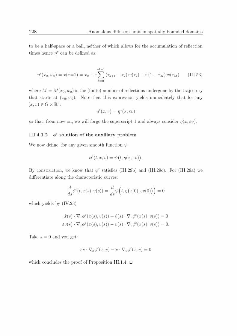
128 Anomalous diffusion limit in spatially bounded domains
to be a half-space or a ball, neither of which allows for the accumulation of reflection
times hence ηε can be defined as:
ηε(x0, w0) = x(τ=1) = x0 + ε
M−1∑
k=0
(τk+1 − τk)w(τk) + ε (1− τM )w(τM) (III.53)
where M =M(x0, w0) is the (finite) number of reflections undergone by the trajectory
that starts at (x0, w0). Note that this expression yields immediately that for any
(x, v) ∈ Ω× Rd:
ηε(x, v) = η1(x, εv)
so that, from now on, we will forgo the superscript 1 and always consider η(x, εv).
III.4.1.2 φε solution of the auxiliary problem
We now define, for any given smooth function ψ:
φε(t, x, v) = ψ(t, η(x, εv)
).
By construction, we know that φε satisfies (III.29b) and (III.29c). For (III.29a) we
differentiate along the characteristic curves:
d
dsφε(t, x(s), v(s)) =
d
dsψ(t, η(x(0), εv(0)
))= 0
which yields by (IV.23)
x(s) · ∇xφε(x(s), v(s)) + v(s) · ∇vφ
ε(x(s), v(s)) = 0
εv(s) · ∇xφε(x(s), v(s))− v(s) · ∇vφ
ε(x(s), v(s)) = 0.
Take s = 0 and you get:
εv · ∇xφε(x, v)− v · ∇vφ
ε(x, v) = 0
which concludes the proof of Proposition III.1.4.
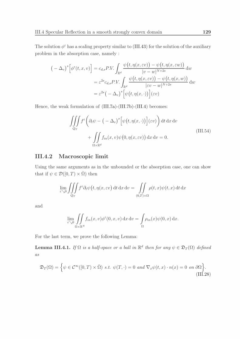
III.4 Specular Reflection in a smooth strongly convex domain 129
The solution φε has a scaling property similar to (III.43) for the solution of the auxiliary
problem in the absorption case, namely :
(−∆v
)s[φε(t, x, v)
]= cd,sP.V.
∫
Rd
ψ(t, η(x, εv)
)− ψ
(t, η(x, εw)
)
|v − w|N+2sdw
= ε2scd,sP.V.
∫
Rd
ψ(t, η(x, εv)
)− ψ
(t, η(x, w)
)
|εv − w|N+2sdw
= ε2s(−∆v
)s[ψ(t, η(x, ·)
)](εv)
Hence, the weak formulation of (III.7a)-(III.7b)-(III.4) becomes:
∫∫∫
QT
f ε(∂tψ −
(−∆v
)s[ψ(t, η(x, ·)
)](εv)
)dt dx dv
+
∫∫
Ω×Rd
fin(x, v)ψ(0, η(x, εv)
)dx dv = 0.
(III.54)
III.4.2 Macroscopic limit
Using the same arguments as in the unbounded or the absorption case, one can show
that if ψ ∈ D([0, T )× Ω) then
limεց0
∫∫∫
QT
f ε∂tψ(t, η(x, εv
)dt dx dv =
∫∫
(0,T )×Ω
ρ(t, x)ψ(t, x) dt dx
and
limεց0
∫∫
Ω×RN
fin(x, v)φε(0, x, v) dx dv =
∫
Ω
ρin(x)ψ(0, x) dx.
For the last term, we prove the following Lemma:
Lemma III.4.1. If Ω is a half-space or a ball in Rd then for any ψ ∈ DT (Ω) defined
as
DT (Ω) =ψ ∈ C∞([0, T )× Ω) s.t. ψ(T, ·) = 0 and ∇xψ(t, x) · n(x) = 0 on ∂Ω
.
(III.28)
130 Anomalous diffusion limit in spatially bounded domains
we have
limεց0
∫∫∫
QT
f ε(−∆v
)s[ψ(t, η(x, ·)
)](εv) dt dx dv =
∫∫
(0,T )×Ω
ρ(t, x)(−∆)sSRψ(t, x) dt dx
(III.55)
where (−∆)sSR
is given in Definition III.33 and can equivalently be written as:
(−∆)sSRψ(t, x) =
(−∆v
)s[ψ(t, η(x, ·)
)](0). (III.56)
Before proving this lemma, which we will do separately for each Ω, let us conclude that
with this convergence we can take the limit in (III.54) and see that for all ψ ∈ DT (Ω)
the macroscopic density ρ(t, x) satisfies
∫∫
(0,T )×Ω
ρ(t, x)(∂tψ(t, x)− (−∆)s
SRψ(t, x)
)dt dx+
∫
Ω
ρin(x)ψ(0, x) dx = 0. (III.57)
which ends the proof of Theorem III.1.5.
III.4.2.1 Lemma III.4.1 in a half-space
Consider the half-space x = (x′, xd) ∈ Rd : xd > 0. The function η associated with
the half-space can be written explicitly as:
η(x, v) =
∣∣∣∣∣x+ v if xd + vd ≥ 0
(x′ + v′,−xd − vd) if xd + vd ≤ 0(III.58)
as illustrated by Figure III.3.
We can differentiate η(x, v) to see that the Jacobian matrix reads
∇vη(x, v) = Id+(H(xd + vd)− 1
)Ed,d (III.59)
where Ed,d is the matrix with 0 everywhere except the last coefficient (of index d, d)
which is 1 and H is the Heaviside function equal to 1 if xd + vd > 0 and −1 if
xd + vd < 0. Furthermore, the second derivative of η(x, v), which we will see as an
element of Md(Rd), i.e. a vector valued matrix, reads
D2vη(x, v) = 2
(n× Ed,d
)δη(x,v)∈∂Ω

III.4 Specular Reflection in a smooth strongly convex domain 131
R+
RN−1
x
(x+ v,−xd − vd)
v
xd + vd
−xd − vd x+ v
Fig. III.3 Example of trajectory in the half-space
where n is the outward unit vector of ∂Ω (which is constant in the half-space), δη(x,v)∈∂Ωis the dirac measure of the boundary surface and × is a multiplication between a vector
u ∈ Rd and a matrix M = (mi,j)1≤i,j≤d ∈ Md(R) whose result is the vector-valued
matrix given by u×M = (mi,ju)1≤i,j≤d ∈ Md(Rd).
Furthermore, a straightforward differentiation yields
D2v
[ψ(t, η(x, v)
)]=(∇vη(x, v)
)TD2ψ
(t, η(x, v)
)(∇vη(x, v)
)+D2
vη(x, v)∇ψ(t, η(x, v)
).
where for any ψ ∈ DT we have
D2vη(x, v)∇ψ
(t, η(x, v)
)= 2(n · ∇ψ
(t, η(x, v)
))Ed,dδη(x,v)∈∂Ω = 0
since for all y = η(x, v) ∈ ∂Ω we have n(y) · ∇ψ(t, y) = 0.
To prove Lemma III.4.1 we will show that(−∆v
)s[ψ(t, η(x, ·)
)](εv) converges strongly
in L∞(0, T ;L2F (v)(Ω × Rd) by a dominated convergence argument. Since f εconverges
weakly in L∞(0, T ;L2F−1(v)(Ω×Rd) we can then pass to the limit in the left-hand-side
of (III.55) and Lemma III.4.1 follows.
We begin by the proof of point-wise convergence. We introduce the function χx :
132 Anomalous diffusion limit in spatially bounded domains
Rd × Rd 7→ R given by (omitting the t variable for the sake of clarity)
χx(v, w) = ψ(η(x, v + w)
)− ψ
(η(x, w)
). (III.60)
For any (t, x, v) ∈ QT we then have
(−∆v
)s[ψ(t, η(x, ·)
)](εv)− (−∆)s
SRψ(x)
= cd,sP.V.
∫
Rd
ψ(t, η(x, εv)
)− ψ
(t, η(x, εv + w)
)
|w|N+2sdw
− cd,sP.V.
∫
Rd
ψ(t, x)− ψ
(t, η(x, w)
)
|w|N+2sdw
= cd,sP.V.
∫
Rd
χx(εv, 0)− χx(εv, w)
|w|d+2sdw. (III.61)
For δ > 0, we split the integral as follow
cd,sP.V.
∫
Rd
χx(εv, 0)− χx(εv, w)
|w|d+2sdw = cd,sP.V.
∫
|w|≤δ
χx(εv, 0)− χx(εv, w)
|w|d+2sdw
+ cd,s
∫
|w|≥δ
χx(εv, 0)− χx(εv, w)
|w|d+2sdw.
On the one hand we see that∣∣∣∣∫
|w|≥δ
χx(εv, 0)− χx(εv, w)
|w|d+2sdw
∣∣∣∣ ≤ 2‖χx(εv, ·)‖L∞(Rd)
∫
|w|≥δ
1
|w|d+2sdw
≤ 2δ−2s‖χx(εv, ·)‖L∞(Rd)
and by definition of χx
supw
|χx(εv, w)| = supw
∣∣∣ψ(η(x, εv + w)
)− ψ
(η(x, w)
)∣∣∣ −→ε→0
0.
so the integral over |w| ≥ δ vanishes. On the other hand, using the symmetry of the
set |w| ≤ δ we write
P.V.
∫
|w|≤δ
χx(εv, 0)− χx(εv, w)
|w|N+2sdw
=1
2P.V.
∫
|w|≤δ
2χx(εv, 0)− χx(εv, w)− χx(εv,−w)|w|d+2s
dw

III.4 Specular Reflection in a smooth strongly convex domain 133
where we can expand χx(εv,±w) using a second-order Taylor-Lagrange expansion
which yields, for some θ and θ in the ball B(δ) centred at the origin with radius δ
2χx(εv, 0)− χx(εv, w)− χx(εv,−w)= −∇wχx(εv, 0) · w − w ·D2χx(εv, θ)w −∇wχx(εv, 0) · (−w)− (−w) ·D2χx(εv, θ)(−w)= −w ·
(D2χx(εv, θ) +D2χx(εv, θ)
)w
therefore
∣∣∣∣P.V.∫
|w|≤δ
χx(εv, 0)− χx(εv, w)
|w|N+2sdw
∣∣∣∣ =1
2
∣∣∣∣∫
|w|≤δ
w(D2χx(εv, θ) +D2χx(εv, θ)
)w
|w|d+2sdw
∣∣∣∣(III.62)
where the P.V. is not needed any more since s < 1. For any fixed θ ∈ B(δ), we have
D2χx(εv, θ) =(∇vη(x, εv + θ)
)TD2ψ
(η(x, εv + θ)
)(∇vη(x, εv + θ)
)
−(∇vη(x, θ)
)TD2ψ
(η(x, θ)
)(∇vη(x, θ)
).
If x+ εv + θ and x+ θ are either both in Ω or both outside Ω then thanks to (III.59)
we know that ∇vη(x, εv + θ) = ∇vη(x, θ). We denote M this matrix and we have
D2χx(εv, θ) =MT(D2ψ
(η(x, εv + θ)
)−D2ψ
(η(x, θ)
))M
in which case the regularity of ψ yields
limε→0
D2χx(εv, θ) = 0.
If x is in the interior of Ω, then for ε and δ small enough, we will obviously have x+ θ
and x + εv + θ inside Ω. Moreover, if x is on the boundary ∂Ω then for any fixed θ
in B(δ), when ε is small enough we will also have x + θ and x + εv + θ either both
inside Ω if w · n(x) < 0 or outside Ω if w · n(x) ≥ 0. As a consequence, we have
point-wise convergence of the integrand in the left side of (III.62) therefore (III.59)
and the regularity of ψ ensure that we can use dominated convergence in L1(B(δ)) to

134 Anomalous diffusion limit in spatially bounded domains
write
limε→0
∣∣∣∣P.V.∫
|w|≤δ
χx(εv, 0)− χx(εv, w)
|w|N+2sdw
∣∣∣∣
=1
2
∣∣∣∣∫
|w|≤δ
limε→0
w(D2χx(εv, θ) +D2χx(εv, θ)
)w
|w|d+2sdw
∣∣∣∣ = 0.
Now that we have proven the point-wise convergence, let us show that
v 7→(−∆v
)s[ψ(t, η(x, ·)
)](εv)
is bounded uniformly in ε by a function in L2F (v)(Ω×Rd). The regularity of ψ and the
above computation of the jacobian matrix of η yield in particular that for all t ∈ [0, T )
supv∈Rd
D2v
[ψ(t, η(x, v)
)]∈ L2(Ω). (III.63)
Therefore, for any t ∈ [0, T ) we introduce Gt(x) given by
Gt(x) = ‖ψ(t, ·)‖L∞(Ω)+∥∥∥D2
v
[ψ(t, η(x, ·)
)]∥∥∥L∞(Rd)
.
As we did before, we can split the integral expression of the fractional Laplacian into a
integral on a ball of radius δ around the singularity and an integral on the complement
of that ball. For the latter, we write for some constant C > 0
∣∣∣∣cd,s∫
Rd\B(δ)
ψ(η(x, εv)
)− ψ
(η(x, εv + w)
)
|w|d+2sdw
∣∣∣∣ ≤ C‖ψ(t, ·)‖L∞(Ω)
∫
Rd\B(δ)
1
|w|d+2sdw
≤ C‖ψ(t, ·)‖L∞(Ω)δ−2s.
For the integral over B(δ), we use a second order Taylor-Lagrange expansion like we
did for χx and write
∣∣∣∣cd,s∫
B(δ)
ψ(η(x, εv)
)− ψ
(η(x, εv + w)
)
|w|d+2sdw
∣∣∣∣
≤ C
∫
B(δ)
w ·(D2[ψ(η(x, ·)
)](εv + θ) +D2
[ψ(η(x, ·)
)](εv + θ)
)w
|w|d+2sdw
≤∥∥∥D2
[ψ(η(x, ·)
)]∥∥∥L∞(Rd)
δ2−2s.
III.4 Specular Reflection in a smooth strongly convex domain 135
Put together we see that for δ = 1 we have for all ε > 0 and v ∈ Rd
∣∣∣∣(−∆v
)s[ψ(t, η(x, ·)
)](εv)
∣∣∣∣ ≤ Gt(x)
and Gt(x) is in L2(Ω) by the previous estimates on the second derivative. Hence, we
have proven that(−∆v
)s[ψ(t, η(x, ·)
)](εv) converges strongly in L∞(0, T ;L2
F (v)(Ω×Rd)) to (−∆)s
SRψ(t, x) and Lemma III.4.1 in the half-space follows.
III.4.2.2 Lemma III.4.1 in a ball
We consider, without loss of generality, that Ω is the unit ball in Rd. For ψ is in
DT (Ω), we will again to prove Lemma III.4.1 by establishing the strong convergence
of(−∆v
)s[ψ(t, η(x, ·)
)](εv) in L∞(0, T ;L2
F (v)(Ω× Rd)) to (−∆)sSRψ(t, x).
First, let us point out that the arguments we presented in the half-space to prove the
point-wise convergence still hold in the ball. Indeed, we can introduce the function
χx defined in (III.60) and split (III.61) over |w| ≤ δ and |w| ≥ δ for some δ > 0. On
the one hand, if we bound the integral over |w| ≥ δ by the L∞-norm of χx in Ω and
the integral of kernel away from its singularity, it follows that this term goes to 0 by
definition of χx and regularity of ψ. On the other hand, the integral over |w| ≤ δ can
be handled exactly the same way as in the half-space. More precisely, if x is away
from the boundary then for δ and ε small enough η(x, εv+w) = x+ εv+w and there
is no issue; and if x is on ∂Ω then we use the fact that locally the boundary of the
ball is isomorphic to the hyperplane xd = 0 so we recover the previous setting and a
dominated convergence argument in L1(B(δ)) will show that the integral over |w| ≤ δ
goes to 0. Together, these two controls and (III.61) prove the point-wise convergence.
The rest of our proof of Lemma III.4.1 requires some estimates on the derivatives of η.
These estimates can be established by a detailed analysis of the trajectories described
by η and we have devoted the Appendix A of this thesis to this analysis. In particular,
in Section A.0.3, we prove the following Lemma:
Lemma III.4.2. For all ψ ∈ DT there exists p > 2 such that
(−∆v
)s[ψ(t, η(x, v)
)]∈ LpF (v)(Ω× R
d).
The strong convergence of(− ∆v
)s[ψ(t, η(x, ·)
)](εv) in L2
F (v)(Ω × Rd) then follows
from the following result
136 Anomalous diffusion limit in spatially bounded domains
Lemma III.4.3. If (hε)ε>0 converges point-wise to h and is bounded in LpF (v)(Ω×Rd)
for some p > 2 uniformly in ε then hε converges strongly to h in L2F (v)(Ω× Rd).
Proof. Consider R > 0 and the ball B(R) of radius R centred at 0 in Rd. The Egorov
theorem states that, since Ω×B(R) is a bounded domain, for any δ > 0 one can find
a subset Aδ ⊂ Ω×B(R) such that |Ω×B(R) \Aδ| ≤ δ and hε converges uniformly
on Aδ which means in particular
∫
Aδ
|hε − h|2F (v) dx dv → 0.
As a consequence, we split the norm as follows
∫∫
Ω×Rd
|hε − h|2F (v) dx dv =∫∫
Aδ
|hε − h|2F (v) dx dv +∫∫
Ω×B(R)\Aδ
|hε − h|2F (v) dx dv
+
∫∫
Ω×Rd\B(R)
|hε − h|2F (v) dx dv.
The first term is handled by Egorov’s theorem. For the second, we write
∣∣∣∣∫∫
Ω×B(R)\Aδ
|hε − h|2F (v) dx dv∣∣∣∣
≤( ∫∫
Ω×B(R)\Aδ
|hε − h|pF (v) dx dv)2/p( ∫∫
Ω×B(R)\Aδ
F (v) dx dv
)1−2/p
≤ C|Ω× B(R) \ Aδ|1−2/p
≤ Cδ1−2/p
and for the third∣∣∣∣
∫∫
Ω×Rd\B(R)
|hε − h|2F (v) dx dv∣∣∣∣
≤( ∫∫
Ω×Rd\B(R)
|hε − h|pF (v) dx dv)2/p( ∫∫
Ω×Rd\B(R)
F (v) dx dv
)1−2/p
≤ C( 1
R2s
)1−2/p
.
III.5 Well posedness of the specular diffusion equation 137
Hence, for any δ > 0 we can find R such that R−2s(1−2/p) ≤ δ/3, δ such that δ1−2/p ≤δ/3 and ε0 such that for all ε ≤ ε0
∫
Aδ
|hε − h|2F (v) dx dv ≤ δ
3
and the lemma follows.
Remark III.4.4. In both the half-space and the ball, when s < 1/2, we do not need to
assume that ∇ψ(x) · n(x) = 0 for all x on the boundary which means we can actually
extend the set of test functions to ψ ∈ C∞([0, T ) × Ω) with ψ(T, ·) = 0. Indeed, in
those cases, η is regular enough to ensure that ψ(t, η(x, v)
)is in H1(Rd) with respect
to the velocity and since H2s(Rd) ⊂ H1(Rd), the fractional Laplacian of order s of
ψ(t, η(x, v)
)will be in L2
F (v)(Ω×Rd). Moreover, in our proof of point-wise convergence
above, if 2s < 1 then we can control the singularity for small w in (III.61) with a first-
order Taylor Lagrange expansion which mean we do not require any assumption on
∇ψ at the boundary.
III.5 Well posedness of the specular diffusion equa-
tion
This last section is devoted to the proof of Theorem III.1.6 and is divided in three steps.
First, we establish some properties of the specular diffusion operator (−∆)sSR
. Secondly,
we handle the first part of Theorem III.1.6 which is the existence and uniqueness of
a weak solution to the specular diffusion equation (III.35a)-(III.35b). Thirdly, we will
show that the distributional solution ρ that we constructed in the previous section is
precisely this unique weak solution when Ω is either the half-space Rd+ = (x, xd) ∈
Rd : xd > 0 or the unit ball B1 in R
d.
Note that although the theorem holds in both domains and the steps are similar in
both cases, the techniques we use at each step often differ so we will have to treat the
cases separately several times.
III.5.1 Properties and estimates of the specular diffusion oper-
ator
III.5.1.1 (−∆)sSR
on the half-space
When Ω is the half-space Rd+, (−∆)s
SRcan be written as a kernel operator
138 Anomalous diffusion limit in spatially bounded domains
Proposition III.5.1. Let us define KRd+
as
KRd+(x, y) = cd,s
(1
|x− y|d+2s+
1
|(x− y, xd + yd)|d+2s
)(III.64)
Then we have
(−∆)sSRψ(x) = P.V.
∫
Rd+
(ψ(x)− ψ(y)
)KRd
+(x, y) dy. (III.34)
Moreover, this kernel is symmetric: KRd+(x, y) = KRd
+(y, x) for all x and y in R
d+ and
satisfies
cd,s1
|x− y|d+2s≤ KRd
+(x, y) ≤ cd,s
2
|x− y|d+2s(III.65)
Proof. The expression for det∇vη(x, v) in the half-space is given by (III.58). Defined
as such, KRd+
is obviously well defined, although singular, and moreover we have:
KRd+(x, y) = cd,s
(1
|x− y|d+2s+
1
|(x− y, xd + yd)|d+2s
)
= cd,s
(1
|y − x|d+2s+
1
|(y − x, yd + xd)|d+2s
)= KRd
+(y, x).
Finally, since 1/|(y − x, yd + xd)|d+2s ≥ 0, the left-hand-side of (III.65) holds and, as
can be seen in Figure III.3, |(x− y, xd+ yd)| ≥ |x− y| which yields the right-hand-side
of (III.65).
In more general domains Ω, we can also try to write (−∆)sSR
as a kernel operator. The
general form of this kernel is given by a generalized change of variable formula, c.f.
[LM95] and reads
KΩ(x, y) = cd,s∑
v∈η−1x (y)
∣∣ det∇vη(x, v)∣∣−1
|v|d+2s. (III.66)
where η−1x (y) = v ∈ Rd : η(x, v) = y. For instance, when Ω is a stripe and a cube,
one can show that the Jacobian determinant of η in those domains is bounded away
from 0, that the sum is infinite but countable and as a consequence that the kernel will
be well defined, symmetric and its singularity will be comparable with the singularity
of(− ∆
)sas expressed in (III.65) for the half-space. Although we won’t dwell on
those domains in this paper, we will make sure not to use the explicit expression of
the kernel in the half-space as long as we can in order to establish results that will
III.5 Well posedness of the specular diffusion equation 139
also hold in any domains where the kernel is well defined, symmetric and 2s-singular.
In particular, we can establish an integration by parts formula for (−∆)sSR
from which
we will deduce its symmetry.
Proposition III.5.2. The operator (−∆)sSR
satisfies an integration by parts formula:
for any ψ and φ smooth enough:
∫
Ω
φ(x)(−∆)sSRψ(x) dx =
1
2
∫∫
Ω×Ω
(φ(x)− φ(y)
)(ψ(x)− ψ(y)
)KΩ(x, y) dx dy. (III.67)
Proof. First, we use the kernel operator expression (III.34) for the (−∆)sSR
operator
and inverse the variables x and y, using the symmetry of the kernel KΩ, in order to
write the following:
∫
Ω
φ(x)(−∆)sSRψ(x) dx =
1
2
∫
x∈Ω
φ(x)P.V.
∫
y∈Ω
(ψ(x)− ψ(y)
)KΩ(x, y) dy dx
− 1
2
∫
y∈Ω
φ(y)P.V.
∫
x∈Ω
(ψ(x)− ψ(y)
)KΩ(x, y) dy dx.
In first integral, we add and subtract (x − y)∇ψ(x)1B(x)(y) where 1B(x)(y) is the
indicator function of a ball around x included in Ω, and we notice that since ψ is
smooth it satisfies for any x ∈ Ω and y ∈ B(x):
ψ(x)− ψ(y)− (x− y)∇ψ(x)1B(x)(y) = O(|x− y|2
)
so that the integral
∫∫
Ω×Ω
φ(x)(ψ(x)− ψ(y)− (x− y)∇ψ(x)1B(x)(y)
)KΩ(x, y) dx dy
is well defined without need of a principal value because the kernel is 2s−singular
with 2s < 2. We do the same in the second integral, adding and subtracting (x −y)∇ψ(y)1B(y)(x) where 1B(y)(x) is the indicator function of a ball around y included

140 Anomalous diffusion limit in spatially bounded domains
in Ω so that we get:
∫
Ω
φ(x)(−∆)sSRψ(x) dx =
1
2
∫∫
Ω×Ω
φ(x)(ψ(x)− ψ(y)− (x− y)∇ψ(x)1B(x)(y)
)KΩ dx dy
+1
2
∫
x∈Ω
φ(x)∇ψ(x)P.V.∫
y∈Ω
(x− y)1B(x)(y)KΩ(x, y) dy dx
− 1
2
∫∫
Ω×Ω
φ(y)(ψ(x)− ψ(y)− (x− y)∇ψ(y)1B(y)(x)
)KΩ(x, y) dx dy
− 1
2
∫
y∈Ω
φ(y)∇ψ(y)P.V.∫
x∈Ω
(x− y)1B(y)(x)KΩ(x, y) dy dx.
Since we can use Fubini’s theorem in the first and the third term, we sum both of
them and notice that(φ(x)− φ(y)
)(ψ(x)− ψ(y)
)= O
(|x− y|2
)in order to write
1
2
∫∫
Ω×Ω
φ(x)(ψ(x)− ψ(y)− (x− y)∇ψ(x)1B(x)(y)
)KΩ(x, y) dx dy
− 1
2
∫∫
Ω×Ω
φ(y)(ψ(x)− ψ(y)− (x− y)∇ψ(y)1B(y)(x)
)KΩ(x, y) dx dy
=1
2
∫∫
Ω×Ω
[(φ(x)− φ(y)
)(ψ(x)− ψ(y)
)− φ(x)∇ψ(x)1B(x)(y)(x− y)
+ φ(y)∇ψ(y)1B(y)(x)(x− y)
]KΩ(x, y) dx dy
=1
2
∫∫
Ω×Ω
(φ(x)− φ(y)
)(ψ(x)− ψ(y)
)KΩ(x, y) dx dy
− 1
2
∫
x∈Ω
φ(x)∇ψ(x)P.V.∫
y∈Ω
(x− y)KΩ(x, y)1B(x)(y) dy dx
+1
2
∫
y∈Ω
φ(y)∇ψ(y)P.V.∫
x∈Ω
(x− y)1B(y)(x)KΩ(x, y) dx dy
which concludes the proof.

III.5 Well posedness of the specular diffusion equation 141
As a direct corollary of this proof, we see that since the kernel KΩ is symmetric, the
operator is symmetric as well:
∫
Ω
φ(x)(−∆)sSRψ(x) dx =
∫
Ω
ψ(x)(−∆)sSRφ(x) dx.
III.5.1.2 (−∆)sSR
on a ball
In the ball, if we wanted to write (−∆)sSR
as a kernel operator using (III.66), the
kernel would only be defined almost everywhere because the determinant of ∇vη is
not bounded away from 0. Indeed, as can be seen in Appendix A, for a fixed x, a fixed
direction θ = v/|v| ∈ Sd−1 and a fixed number of reflections, we can find one and only
one norm |v| such that the determinant of ∇xη(x, |v|θ) is null. This can be seen in the
expression (A.9) because finding this norm is equivalent to solving det∇vη(x, v) = 0
after fixing all the variables except lend and, in that setting, the Jacobian determinant
is a monotonous function of lend that passes through 0. However, for each fixed x, the
set of velocities v such that the determinant is null is a countable sum of curves since
for each fixed number of reflections k there is exactly one v in that set per direction θ
in Sd−1. Therefore, the kernel is defined almost everywhere.
Nevertheless, even if we can’t rigorously write it with a kernel, the specular diffusion
operator still has interesting properties, as for instance:
Proposition III.5.3. When Ω is a ball B, the operator (−∆)sSR
admits the following
integration by parts formula: for all φ and ψ smooth enough
∫
Ω
φ(x)(−∆)sSRψ(x) dx =
1
2cd,s
∫∫
Ω×Rd
(φ(x)− φ
(η(x, v)
))(ψ(x)− ψ(η(x, v)
)) dv dx
|v|d+2s.
(III.68)
From which we readily deduce its symmetry
∫
Ω
φ(x)(−∆)sSRψ(x) dx =
∫
Ω
ψ(x)(−∆)sSRφ(x) dx (III.69)

142 Anomalous diffusion limit in spatially bounded domains
Proof. We write
∫
Ω
φ(x)(−∆)sSRψ(x) dx = cd,s
∫∫
Ω×Rd
(φ(x)− φ
(η(x, v)
))(ψ(x)− ψ(η(x, v)
)) dv dx
|v|d+2s
− cd,sP.V.
∫∫
Ω×Rd
φ(η(x, v)
)(ψ(x)− ψ
(η(x, v)
)) dv dx
|v|d+2s.
In the second term on the right-hand-side we want to do a change of variable F (x, v) =
(y, w) such that the trajectory described by η from (y, w) is exactly the trajectory from
(x, v) backwards. In particular, that means η(y, w) = x and η(x, v) = y. We have the
following result on this change of variable which will be proven in Section A.0.4 of the
appendices:
Lemma III.5.4. The change for variable F given by
F
(x
v
)=
(η(x, v)
−[∇vη(x, v)
]v
)(III.70)
is precisely the change of variable such that η(F (x, v)) = x and the trajectory described
by η starting at η(x, v) with velocity −[∇vη(x, v)
]v is exactly the trajectory from (x, v)
backwards. Moreover, for all (x, v):
det∇F (x, v) = 1. (III.71)
The singularity that requires the principal value is at v = 0 around which we have
explicitly η(x, v) = x + v hence it will become, through the change of variable, a
singularity at w = 0 since we have w = −v in the neighbourhood of 0. The change
of variables yields
∫
Ω
φ(x)(−∆)sSRψ(x) dx = cd,s
∫∫
Ω×Rd
(φ(x)− φ
(η(x, v)
))(ψ(x)− ψ(η(x, v)
)) dv dx
|v|d+2s
− cd,sP.V.
∫∫
Ω×Rd
φ(y)(ψ(η(y, w)
)− ψ(y)
) dw dy
|w|d+2s
and the integration by parts formula follows.
III.5 Well posedness of the specular diffusion equation 143
Finally, in relation with (III.65), one can see immediately from looking at the integra-
tion by part formula in a ball, that the singularity in the operator is of order exactly
2s.
III.5.1.3 The Hilbert space HsSR(Ω)
We conclude the analysis of (−∆)sSR
by introducing the associated Hilbert space
HsSR(Ω). This comes down to interpreting the integration by parts formula as a type of
scalar product and considering the associated semi-norm in the spirit of the Gagliardo
(semi-)norm on the fractional Sobolev space Hs(Rd) and its relation with the fractional
Laplacian as presented e.g. in [DPV12]. The natural semi-norm associated with the
specular diffusion operator reads in the half-space
[ψ]2HsSR
(Rd+) =
1
2
∫∫
Rd+×Rd
+
(ψ(x)− ψ(y)
)2KRd
+(x, y) dx dy.
and in the ball
[ψ]2HsSR
(B) =cd,s2
∫∫
Rd×B
(ψ(x)− ψ
(η(x, v)
))2 1
|v|d+2sdx dv.
Consequently, we introduce a Hilbert space associated with the specular diffusion
operator.
Definition III.5.1. We define the Hilbert space HsSR(Ω) as
HsSR(Ω) =
ψ ∈ L2(Ω) : [ψ]Hs
SR(Ω) <∞
(III.72)
associated with a scalar product which, on a half-space, read
〈ψ|φ〉HsSR
(Rd+) =
∫
Rd+
ψφ dx+1
2
∫∫
Rd+×Rd
+
(φ(t, x)− φ(t, y)
)(ψ(t, x)− ψ(t, y)
)KRd
+(x, y) dx dy
(III.73)

144 Anomalous diffusion limit in spatially bounded domains
and on the ball becomes
〈ψ|φ〉HsSR
(B) =
∫
B
ψφ dx
+cd,s2
∫∫
Rd×B
(φ(t, x)− φ
(t, η(x, v)
))(ψ(t, x)− ψ
(t, η(x, v)
)) dx dv
|v|d+2s
(III.74)
hence the norm associated with HsSR(Ω) is naturally
‖ψ‖2HsSR
(Ω)= ‖ψ‖2L2(Ω)+[ψ]2HsSR
(Ω)
This functional space is strongly linked with the Sobolev space Hs(Ω) and we refer the
interested reader to [DPV12] for more details. We notice right away that (−∆)sSR
is
self-adjoint on the Hilbert space HsSR(Ω) and also, by the estimates on the singularity
of the operator established above, we see that HsSR(Ω) ⊂ Hs(Ω).
III.5.2 Existence and uniqueness of a weak solution for the
macroscopic equation
We now turn to the specular diffusion equation (III.35a)-(III.35b).
Theorem III.1.6 (Part I). Let Ω be a half-space or a ball in Rd, uin be in L2((0, T )×Ω) and s be in (0, 1). For any T > 0, there exists a unique weak solution u ∈L2(0, T ;Hs
SR(Ω)) of
∂tu+ (−∆)sSRu = 0 (t, x) ∈ [0, T )× Ω (III.35a)
u(0, x) = uin(x) x ∈ Ω (III.35b)
in the sense that for any ψ ∈ DT defined in (III.28), u satisfies if Ω is a half-space:
∫∫
(0,T )×Ω
u∂tψ dt dx−∫
Ω
uin(x)ψ(0, x) dx
− 1
2
∫∫∫
(0,T )×Ω×Ω
(u(t, x)− u(t, y)
)(ψ(t, x)− ψ(t, y)
)K(x, y) dt dx dy = 0.
(III.36)

III.5 Well posedness of the specular diffusion equation 145
and if Ω is the unit ball
∫∫
(0,T )×Ω
u∂tψ dt dx−∫
Ω
uin(x)ψ(0, x) dx
− 1
2
∫∫∫
(0,T )×Ω×Rd
(u(t, x)− u
(t, η(x, v)
))(ψ(t, x)− ψ
(t, η(x, v)
)) dt dx dv|v|d+2s
= 0.
(III.37)
Proof of Theorem III.1.6, (Part I). This proof is strongly inspired by the proof of exis-
tence and uniqueness of weak solutions to the Vlasov-Poisson-Fokker-Planck equation
from Carrillo [Car98]. We consider an associated problem which comes formally from
deriving (III.35a) for u(t, x) = e−λtu(t, x) for some λ > 0:
∂tu(t, x) + λu(t, x) + (−∆)sSRu(t, x) = 0 (t, x) ∈ (0, T )× Ω
u(0, x) = uin(x) x ∈ Ω.(III.76)
Note that we do not prescribe any explicit boundary condition on ∂Ω. A weak solution
of (III.76) is a function u ∈ L2(0, T ;HsSR(Ω)) such that for any ψ ∈ DT ,
∫∫
(0,T )×Ω
(− u∂tψ + λuψ + u(−∆)s
SRψ)dt dx+
∫
Ω
uin(x)ψ(0, x) dx = 0.
We first prove existence of weak solutions of this problem using a Lax-Milgram argu-
ment and we will show afterwards that it implies existence for (III.35a)-(III.35b). We
consider on DT the prehilbertian norm
|ψ|2DT
= ‖ψ‖2HsSR
(Ω)+1
2‖ψ(0, ·)‖2L2(Ω).
We then introduce the bilinear form a from L2(0, T ;HsSR(Ω))×DT to R defined as
a(u, ψ) =
∫∫
(0,T )×Ω
(− u∂tψ + λuψ + u(−∆)s
SRψ)dt dx
and the continuous bounded linear operator L on F :
L(ψ) =
∫
Ω
uin(x)ψ(0, x) dx.
146 Anomalous diffusion limit in spatially bounded domains
From Lemma III.4.2 we know in particular that DT is a subset of L2(0, T ;HsSR(Ω))
with a continuous injection. Moreover, it is easy to see that a is continuous and it is
also coercive since:
a(ψ, ψ) =
∫∫
(0,T )×Rd
λψ2 + ψ(−∆)sSRψ dt dx+
1
2
∫
Ω
ψ(0, x)2 dx ≥ min(1, λ)|ψ|2DT
hence, the Lax-Milgram theorem gives us existence of a weak solution of (III.76) in
L2(0, T ;HsSR(Ω)). From this weak solution ψ we define ψ(t, x) = e−λtψ(t, x) which
is obviously in L2(0, T ;HsSR(Ω)) and weak solution of (III.35a)-(III.35b). Since the
equation is linear, to show uniqueness is equivalent to proving that the only weak
solution with initial data uin = 0 is the zero function. Call u0 this weak solution.
Multiplying (III.35a) by u0 and integrating over Ω we have:
∫
Ω
1
2∂t(u20)dx = −
∫
Ω
u0(−∆)sSRu0 dx ≤ 0.
Hence ‖u0(t, ·)‖L2(Ω) is decreasing. Since it was 0 to start with, that means u0 ≡ 0
and that concludes the proof of uniqueness of solution. Finally, we notice that the
integration by parts formula (III.67) concludes the proof existence and uniqueness of
a weak solution of (III.35a)-(III.35b) in the sense given in Theorem III.1.6.
III.5.3 Identifying the macroscopic density as the unique weak
solution
Finally, we turn to the last part of Theorem III.1.6
Theorem III.1.6 (Part II). If Ω is a ball or a half-space, the macroscopic density
ρ who satisfies (III.32) for all ψ ∈ DT (Ω) is the unique weak solution of (III.35a)-
(III.35b).
Proof. In order to prove this theorem we will show that there is a unique distributional
solution of (III.32), i.e. a unique ρ such that (III.32) holds for all ψ ∈ DT (Ω). Indeed,
since it is obvious that the weak solution of (III.35a)-(III.35b) is also a distributional
solution of (III.32), if we prove its uniqueness then Theorem III.1.6 Part II will follow
immediately.
As usual, to prove uniqueness for linear PDEs, we assume that there are two distri-
butional solutions ρ1 and ρ2 or (III.32) and we consider their difference ρ = ρ1 − ρ2

III.5 Well posedness of the specular diffusion equation 147
which satisfies for any ψ in DT
∫∫
[0,T )×Ω
ρ(∂tψ − (−∆)s
SRψ)dt dx = 0 (III.77)
with∫Ωρ dx = 0 thanks to the conservation of mass. We want to prove that ρ is null.
In order to do so, we first introduce the following reverse evolution problem and show
its wellposedness:
Proposition III.5.5. For any ρ ∈ L∞([0, T );L2(Ω)) there exists a unique ψρ weak
solution in L2((0, T )× Ω) of:
∂tψρ − (−∆)s
SRψρ = ρ (t, x) ∈ [0, T )× Ω
ψρ(T, x) = 0 x ∈ Ω(III.78)
Proof. The proof of part 1 of Theorem III.1.6 above can easily be adapted to show
existence of uniqueness of weak solution in L2(0, T ;HsSR(Ω)) of (III.35a)-(III.35b) with
a source term S, namely:
∂tu+ (−∆)sSRu = S(t, x) (t, x) ∈ [0, T )× Ω
u(0, x) = uin(x) x ∈ Ω.
To do so, one only needs to change the continuous bounded linear map L to
L(ψ) =
∫
Ω
uin(x)ψ(0, x) dx+
∫∫
(0,T )×Ω
Sψ dt dx
where S(t, x) = e−λtS(t, x), and the rest of the proof holds. Hence, if we consider
this weak solution u and define ψρ(t, x) = u(T − t, x) as well as choose S such that
ρ(t, x) = −S(T − t, x) and take uin = 0, this gives us the unique ψρ weak solution of
(III.78) in L2(0, T ;HsSR(Ω)).
We see now that if we can use ψρ as a test function in (III.77) then we will have
∫∫
[0,T )×Ω
ρ2 dx dt = 0
which concludes the proof of uniqueness of the distributional solution ρ of (III.57). It
remains to show that ψρ is an admissible test function for (III.32).

148 Anomalous diffusion limit in spatially bounded domains
When Ω is a ball or a half-space and s < 1/2, as stated in Remark III.4.4, we don’t
need to control the second derivative of ψ(t, η(x, v)) in order to take the limit in
the weak formulation (III.54) so we can actually extend the set of test functions to
C∞([0, T )× Ω) which is dense in L∞([0, T );HsSR(Ω)) with respect to the Hs
SR-norm and
the result is immediate.
When s > 1/2, however, the test functions in (III.77) need to be in DT so we need to
understand the behaviour of ψρ on the boundary. Let us recall that DT is defined as:
DT (Ω) =ψ ∈ C∞([0, T )× Ω) s.t. ψ(T, ·) = 0 and ∀x ∈ ∂Ω : ∇xψ(t, x) · n(x) = 0
.
The interaction between the singularity in the specular diffusion operator and the
boundary leads us to believe that ψρ satisfies a rather strong, non-local boundary
condition but we are unable to write this condition explicitly since it is contained in
the action of (−∆)sSR
. As a consequence, we will show instead that ψρ satisfies, in
particular, an homogeneous Neumann condition. To that end, we first regularize with
respect to time the right hand side of (III.78), and call n the regularizing parameter.
For each n, since the operator (−∆)sSR
is self-adjoint and dissipative it generates a
strongly continuous semi-group of contractions and as a consequence one can prove,
see [Paz83] Section 4.2 for more details, that there exists a unique strong solution ψnof (III.78) which, in particular, satisfies for any t
(−∆)sSRψn(t, x) ∈ L∞(Ω). (III.79)
Moreover, we have the following lemma:
Lemma III.5.6. Let Ω be a ball or a half-space and s > 1/2. For any ψ such that
(−∆)sSRψ(x) ∈ L∞(Ω), we have
∇xψ(t, x) · n(x) = 0 ∀x ∈ ∂Ω. (III.80)
Postponing the proof of this lemma, let us conclude the proof of Theorem III.1.6. For
each ψn, since it satisfies (III.80), we know that if it was in H2(Ω) then we could
approach it by functions in DT with respect to the H2-norm. Moreover, ψn is a strong
solution of (III.78) which entails that it belongs at least to H2sSR(Ω) because (−∆)s
SRψn
is in L2(Ω). Further, as stated before, H2sSR(Ω) ⊂ H2s(Ω), and since s < 1 that means
we can approach ψn by functions in DT with respect to the H2sSR(Ω)-norm, which is
strong enough to take the limit in (III.77). Hence, ψρ is an admissible test function
for (III.77), which yields the uniqueness of the distributional solution of (III.57).
III.5 Well posedness of the specular diffusion equation 149
Proof of Lemma III.5.6. For the half-space, we notice that (−∆)sSRψ can be inter-
preted as the fractional Laplacian acting on its mirror-extension ψ defined as:
ψ(t, x) =
∣∣∣∣∣ψ(t, x) if xd ≥ 0
ψ(t, [x′,−xd]) if xd ≤ 0(III.81)
where we wrote x = (x′, xd) with x′ ∈ Rd−1. The boundary behaviours of ψ follows
readily because we know that in order for(− ∆
)sψ to be bounded, ψ has to be at
least C1,2s−1 on Rd. Since it is a mirror-extension that means ψ has to satisfy an
homogeneous Neumann condition on the boundary:
∇xψ(t, x) · n(x) = 0 ∀x ∈ ∂Ω.
Note that the same line of argument would also hold in a stripe or a cube since we can
define in those cases an extension that consists of a composition of mirror extensions
and such that (−∆)sSRψ coincides with the action of
(−∆
)son that extension.
When Ω is a ball, since (−∆)sSRψ(x) ∈ L∞(Ω), we have
∫
Rd
[ψn(x)− ψn
(η(x, v)
)−∇ψn(x) ·
(η(x, v)− x
)] dv
|v|d+2s
+ P.V.
∫
Rd
∇ψn(x) ·(η(x, v)− x
) dv
|v|d+2s
is in L∞(Ω). In the first integral
ψn(x)− ψn(η(x, v)
)−∇ψn(x) ·
(η(x, v)− x
)= O(|x− η(x, v)|2)
which means the integral is finite since 2s < 2. Hence, we have
∇ψn(x) · P.V.∫
Rd
(η(x, v)− x
) dv
|v|d+2s∈ L∞(Ω) (III.82)
Let us show that there is a function f(x) such that
P.V.
∫
Rd
(η(x, v)− x
) dv
|v|d+2s= f(x)n(x) with f(x) →
x→∂Ω−∞ (III.83)

150 Anomalous diffusion limit in spatially bounded domains
where n(x) denotes the extended outward normal vector: n(x) = x/|x| if x 6= 0. We
write the integral in a orthonormal coordinates system that starts with e1 = n(x) and
with the notation η(x, v) =∑ηi(x, v)ei. We have:
P.V.
∫
Rd
(η(x, v)− x
) dv
|v|d+2s=
(P.V.
∫
Rd
(η1(x, v)− |x|
) dv
|v|d+2s
)e1
+∑
2≤i≤d
(P.V.
∫
Rd
ηi(x, v)dv
|v|d+2s
)ei
:= I1n(x) +∑
2≤i≤d
Iiei.
For the coefficient I2 we notice that if we call T2 : y ∈ Rd 7→ y − 2y2e2, the mirror
image of y with respect to the hyperplane y2 = 0, then it is easy to see that the ball
is invariant by T2: T2(B1) = B1 which means that η acts in T2(B1) exactly as it acts
on B1. As a consequence, T2 and η commute: η(x, T2v) = T2η(x, v) which yields:
I2 = limε→0
∫∫
|v1|≥ε×Rd−2
( ∫
v2>0
η2(x, v)dv2
|v|d+2s+
∫
v2<0
η2(x, v)dv2
|v|d+2s
)dv1 dv3 · · · dvd
= limε→0
∫∫
|v1|≥ε×Rd−2
( ∫
v2>0
η2(x, v)dv2
|v|d+2s+
∫
v2>0
(η2(x, Tv))dv2
|v|d+2s
)dv1 dv3 · · · dvd
= limε→0
∫∫
|v1|≥ε×Rd−2
( ∫
v2>0
η2(x, v)dv2
|v|d+2s+
∫
v2>0
(−η2(x, v))dv2
|v|d+2s
)dv1 dv3 · · · dvd
= 0.
The same holds for all Ii, i ≥ 2 so that we can define a function f(x) = I1 with which
P.V.
∫
Rd
(η(x, v)− x
) dv
|v|d+2s=
(P.V.
∫
Rd
(η1(x, v)− |x|
) dv
|v|d+2s
)n(x) := f(x)n(x).
To understand the behaviour of f as x goes to the boundary we split the integral as
follows, for some R > 0 fixed, writing B1−|x| the ball centred at 0 of radius 1−|x| and
III.5 Well posedness of the specular diffusion equation 151
CR the cube centred at 0 of side 2R (assuming w.l.o.g. that R > 1− |x|):
f(x) =P.V.
∫
B1−|x|
((η1(x, v)− |x|
) dv
|v|d+2s
+
∫
CR\B1−|x|
(η1(x, v)− |x|
) dv
|v|d+2s+
∫
Rd\CR
(η1(x, v)− |x|
) dv
|v|d+2s.
For the first term on the right-hand-side, we use the explicit expression of η when
there are no reflections: η(x, v) = x+ v in order to write
P.V.
∫
B1−|x|
((η1(x, v)− |x|
) dv
|v|d+2s= lim
ε→0
∫
ε<|v|<1−|x|
v1dv
|v|d+2s= 0
because the integrand is an odd function and the domain is radially symmetric. For
the last term in the expression of f(x) we write
∣∣∣∣∫
Rd\CR
(η1(x, v)− |x|
) dv
|v|d+2s
∣∣∣∣ ≤∫
|v|>R
|v||v|d+2s
dv =1
2sR2s−1
which is fixed with R. Finally, for the second term in the expression of f(x), we want
to identify a sign in the integrand to which end we introduce
E(x) =(CR \B1−|x|
)∩(
−R ≤ v1 ≤ 0∪2(1− |x|) ≤ v1 ≤ R
)
so that for any v ∈ E(x) we have η1(x, v)−|x| ≤ 0 (note that the set of all velocities such
that η1(x, v) − |x| ≤ 0 is actually a little bigger that E(x) because of the curvature
of ∂Ω, if ∂Ω was a straight line that it would be precisely E(x)). We also write
E c(x) = (CR \B1−|x|) \ E(x) its complement in CR \B1−|x| with which we have
∫
CR\B1−|x|
(η1(x, v)− |x|
) dv
|v|d+2s= −
∫
E(x)
∣∣η1(x, v)− x∣∣ dv
|v|d+2s+
∫
Ec(x)
(η1(x, v)− x
) dv
|v|d+2s.
We introduce the notations
E(x, v1) =(v2, · · · , vd) :
√(1− |x|)2 − v21 ≤ |v2|, · · · , |vd| ≤ R

152 Anomalous diffusion limit in spatially bounded domains
and
E c(x, v1) =(v2, · · · , vd) :
√(1− x)2 − v21 ≤ |v2|, · · · , |vd| ≤ 2(1− |x|)
such that for a fixed v1 the projection of E(x) on w ∈ Rd : w1 = v1 is E(x, v1) if
−R ≤ v1 ≤ 0 and [−R,R]d−1 if 2(1 − |x|) ≤ v1 ≤ R, and the projection of E c(x) is
E c(x, v1). With those, we have on the one hand
∫
E(x)
∣∣η1(x, v)− x∣∣ dv
|v|d+2s=
|x|∫
v1=−R
( ∫
E(x,v1)
∣∣η1(x, v)− x∣∣
|v|d+2sdv2 · · · dvd
)dv1
+
R∫
v1=2(1−|x|)
( ∫
[−R,R]d−1
∣∣η1(x, v)− x∣∣
|v|d+2sdv2 · · · dvd
)dv1
and on the other hand
∣∣∣∣∫
Ec(x)
(η1(x, v)− x
) dv
|v|d+2s
∣∣∣∣ ≤2(1−|x|)∫
v1=0
( ∫
Ec(x,v1)
∣∣η1(x, v)− x∣∣
|v|d+2sdv2 · · · dvd
)dv1.
We see that it is the same integrand but in the integral over E c(x), the volume of the
domain of integration(0, 2(1−|x|)
)×E c(x, v1) goes to 0 as x approaches the boundary
whereas the domains (−R, |x|)×E(x, v1) and(2(1−|x|), R)× (−R,R)2 do not, hence
the first term is negligible in the limit before the second and we have
|f(x)| ∼x→∂Ω
∫
E(x)
∣∣η1(x, v)− x∣∣ dv
|v|d+2s≥
|x|∫
v1=−R
( ∫∫
E(x,v1)
v1|v|d+2s
dv2 dv3
)dv1
≥∫∫
1−|x|≤|v2|,|v3|≤R
(|x|−1∫
−R
v1|v|d+2s
)dv2 dv3
≥∫∫
1−|x|≤|v2|,|v3|≤R
C((1− |x|)2 + v22 + v23
)(d+2s−2)/2dv2 dv3.
As x approaches the boundary, the integrand tends to 1/(v22 + v23)d−1+2s−1 and the
domain to [−R,R]d−1 so the integral diverges since 2s− 1 > 0.
Chapter IV
Classical diffusion limit in spatially
bounded domains
Joint work with Harsha Hutridurga
Diffusion limit for Vlasov-Fokker-Planck equation in bounded domainsarXiv:1604.08388 (2016).
Contents
IV.1 Introduction . . . . . . . . . . . . . . . . . . . . . . . . . . . 154
IV.1.1 The Vlasov-Fokker-Planck equation . . . . . . . . . . . . . . 154
IV.1.2 Main result . . . . . . . . . . . . . . . . . . . . . . . . . . . 156
IV.1.3 Plan of the paper . . . . . . . . . . . . . . . . . . . . . . . . 157
IV.2 Strategy of the proof . . . . . . . . . . . . . . . . . . . . . . 157
IV.2.1 Efficiency of our approach . . . . . . . . . . . . . . . . . . . 159
IV.3 Solutions of the Vlasov-Fokker-Planck equation . . . . . . 160
IV.3.1 Existence of weak solution . . . . . . . . . . . . . . . . . . . 161
IV.3.2 Uniform a priori estimate . . . . . . . . . . . . . . . . . . . 163
IV.4 Auxiliary problem . . . . . . . . . . . . . . . . . . . . . . . . 165
IV.4.1 Geodesic Billiards and Specular cycles . . . . . . . . . . . . 166
IV.4.2 Solution to the auxiliary problem and rescaling . . . . . . . 168
IV.5 Derivation of the macroscopic model . . . . . . . . . . . . . 169

154 Classical diffusion limit
IV.1 Introduction
IV.1.1 The Vlasov-Fokker-Planck equation
In this paper, we study the diffusion limit of Vlasov-Fokker-Planck equation in a
bounded spatial domain with specular reflections on the boundary. The equation we
consider models the behavior of a low density gas in the absence of macroscopic force
field. Introducing the probability density f(t, x, v), i.e., the probability of finding a
particle with velocity v at time t and position x, we consider the evolution equation
∂tf + v · ∇xf = Lf := ∇v ·(∇vf + vf
)for (t, x, v) ∈ (0, T )× Ω× R
d, (IV.1a)
f(0, x, v) = f in(x, v) for (x, v) ∈ Ω× Rd. (IV.1b)
The left hand side of (IV.1a) models the free transport of particles, while the Fokker-
Planck operator L on the right hand side describes the interaction of the particles with
the background. It can be interpreted as a deterministic description of a Langevin
equation for the velocity of the particles:
v(t) = −νv(t) +W (t),
where the friction coefficient ν will be assumed, without loss of generality, equal to
1 and W (t) is a Gaussian white noise. We consider (IV.1a) on a smooth bounded
domain Ω ⊂ Rd in the sense that there exists a smooth function ζ : Rd 7→ R such that
Ω = x ∈ Rd s.t. ζ(x) < 0; ∂Ω = x ∈ R
d s.t. ζ(x) = 0. (IV.2)
In order to define a normal vector at each point on the boundary we assume that
∇xζ(x) 6= 0 for any x such that ζ(x) ≪ 1 and we define the unit outward normal
vector, for any x ∈ ∂Ω, as
n(x) :=∇xζ(x)
|∇xζ(x)|.
Moreover, we also assume that Ω is strongly convex, namely that there exists a constant
Cζ > 0 such that
d∑
i,j=1
ξi∂2ζ
∂xi∂xjξj ≥ Cζ|ξ|2 ∀ ξ ∈ R
d. (IV.3)
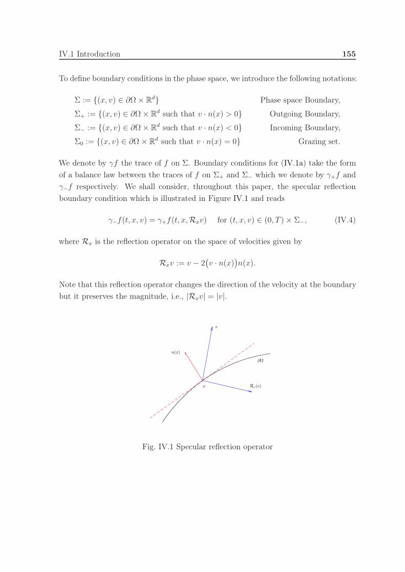
IV.1 Introduction 155
To define boundary conditions in the phase space, we introduce the following notations:
Σ := (x, v) ∈ ∂Ω× Rd Phase space Boundary,
Σ+ := (x, v) ∈ ∂Ω× Rd such that v · n(x) > 0 Outgoing Boundary,
Σ− := (x, v) ∈ ∂Ω× Rd such that v · n(x) < 0 Incoming Boundary,
Σ0 := (x, v) ∈ ∂Ω × Rd such that v · n(x) = 0 Grazing set.
We denote by γf the trace of f on Σ. Boundary conditions for (IV.1a) take the form
of a balance law between the traces of f on Σ+ and Σ− which we denote by γ+f and
γ−f respectively. We shall consider, throughout this paper, the specular reflection
boundary condition which is illustrated in Figure IV.1 and reads
γ−f(t, x, v) = γ+f(t, x,Rxv) for (t, x, v) ∈ (0, T )× Σ−, (IV.4)
where Rx is the reflection operator on the space of velocities given by
Rxv := v − 2(v · n(x)
)n(x).
Note that this reflection operator changes the direction of the velocity at the boundary
but it preserves the magnitude, i.e., |Rxv| = |v|.
v
Rx(v)x
n(x)
∂Ω
Fig. IV.1 Specular reflection operator

156 Classical diffusion limit
IV.1.2 Main result
In order to investigate the diffusion limit of (IV.1a)-(IV.1b), we introduce the Knudsen
number 0 < ε≪ 1 which represents the ratio of the mean free path to the macroscopic
length scale, or equivalently the ratio of the mean time between two kinetic interactions
to the macroscopic time scale. We rescale time as t′ = εt and also introduce a coefficient
ε−1 in front of the Fokker-Planck operator in (IV.1a) to model the number of collision
per unit of time going to infinity. The rescaled equation, thus becomes
ε∂tfε + v · ∇xf
ε =1
ε∇v · (vf ε +∇vf
ε) for (t, x, v) ∈ (0, T )× Ω× Rd, (IV.5a)
f ε(0, x, v) = f in(x, v) for (x, v) ∈ Ω× Rd, (IV.5b)
γ−fε(t, x, v) = γ+f
ε (t, x,Rxv) for (t, x, v) ∈ (0, T )× Σ−. (IV.5c)
In this paper, we investigate the behavior of the solution f ε in the ε → 0 limit. The
characterization of the asymptotic behavior of f ε(t, x, v) is the object of our main
result.
Theorem IV.1.1. Assume the initial datum f in(x, v) satisfies
f in(x, v) ≥ 0 ∀(x, v) ∈ Ω× Rd; f in ∈ L2
(Ω× R
d,M−1(v)dxdv),
where M(v) is the centered Gaussian
M(v) :=1
(2π)d/2e
−|v|2
2 . (IV.6)
Let f ε(t, x, v) be a weak solution to the initial boundary value problem (IV.5a)-(IV.5b)-
(IV.5c). Then
f ε(t, x, v) ρ(t, x)M(v) in L∞(0, T ; L2
(Ω× R
d,M−1(v)dvdx))
weak-*
as ε → 0, for some ρ ∈ L∞(0, T ; L2(Ω)). Furthermore, if the spatial domain Ω is a
ball in Rd then the limit ρ(t, x) is a weak solution to the diffusion equation
∂tρ−∆xρ = 0 for (t, x) ∈ (0, T )× Ω, (IV.7a)
ρ(0, x) = ρin(x) for x ∈ Ω, (IV.7b)
∇xρ(t, x) · n(x) = 0 for (t, x) ∈ (0, T )× ∂Ω, (IV.7c)

IV.2 Strategy of the proof 157
with the initial datum
ρin(x) =
∫
Rd
f in(x, v) dv.
IV.1.3 Plan of the paper
Section IV.2 gives some heuristics with regard to the strategy of proof for Theorem
IV.1.1. In particular, we compare our method of proof with some standard techniques
used to prove the diffusion limit for the kinetic Fokker-Planck equation. In section IV.3,
we define an appropriate notion of weak solution to our initial boundary value problem.
In section IV.4, we develop the theory of constructing a special class of test functions
using an auxiliary problem. Finally, in section IV.5, we arrive at the parabolic limit
equation, thus proving Theorem IV.1.1. In the Appendix, and especially section A.0.5
we give regularity results associated with some Hamiltonian dynamics that we will
need to study the aforementioned auxiliary problem.
Acknowledgments. The authors would like to acknowledge the support of the ERC
grant matkit. H.H. also acknowledges the support of the EPSRC programme grant
“Mathematical fundamentals of Metamaterials for multiscale Physics and Mechanic”
(EP/L024926/1). The authors would like to thank Antoine Mellet for his fruitful
suggestions on a preliminary version of this manuscript. The authors also extend their
humble thanks to Clément Mouhot for interesting discussions on this problem.
IV.2 Strategy of the proof
In this section, we lay out the strategy of our proof for Theorem IV.1.1. We would
like to demonstrate the novelty in our approach by citing some comparisons with
the standard techniques used in the diffusion approximation for the Vlasov-Fokker-
Planck equation. Those techniques were introduced in 1987 by Degond and Mas-
Gallic [DMG87] for the one dimensional case in bounded domains. They were later
improved, in 2000, by Poupaud and Soler [PS00] where they consider the more com-
plicated Vlasov-Poisson-Fokker-Planck equation on the whole space and established
the diffusion limit for a small enough time interval. More recently, improving the
result further, Goudon [Gou05] established in 2005 the global-in-time convergence in
dimension 2 with bounds on the entropy and energy of the initial data so as to ensure
that singularities do not develop in the limit system and finally, in 2010, El Ghani and

158 Classical diffusion limit
Masmoudi proved in [EGM10] the global-in-time convergence in higher dimensions
with similar initial bounds.
In these papers, the analysis with regard to this nonlinear model is quite involved. Let
us simply present the analysis in [PS00] adapted to the linear model (IV.5a). The idea
is to consider the continuity equation for the local densities ρε(t, x) given by
∂ρε
∂t(t, x) +
1
ε∇x · jε(t, x) = 0,
where the current density jε(t, x) is defined as
jε(t, x) :=
∫
Rd
vf ε(t, x, v) dv.
The principal idea is to obtain
ρε ρ weakly in L1((0, T )× Ω),
1
εjε ∇xρ in D′((0, T )× Ω)
(IV.8)
as ε→ 0. The article [PS00] is concerned with the analysis in the full spatial domain
Rd. In order to derive the limit boundary condition – we refer the interested reader
to the paper [WLL15b] of Wu, Lin and Liu for more details – one can multiply the
specular reflection boundary condition (IV.5c) by (v · n(x)) and integrate over the
incoming velocities at the point x ∈ ∂Ω yielding
∫
v·n(x)<0
γ−fε(t, x, v) (v · n(x)) dv =
∫
v·n(x)<0
γ+fε(t, x,Rx(v)) (v · n(x)) dv.
Making the change of variables w = Rx(v) on the right hand side of the above expres-
sion yields
∫
v·n(x)<0
γ−fε(t, x, v) (v · n(x)) dv = −
∫
w·n(x)>0
γ+fε(t, x, w) (w · n(x)) dw.
This implies the following
∫
Rd
γf ε (v · n(x)) dv = 0 =⇒ jε(t, x) · n(x) = 0.
IV.2 Strategy of the proof 159
Taking the limits (IV.8) into consideration, we do have the homogeneous Neumann
condition on the boundary in the ε → 0 limit.
Our strategy is essentially different in the sense that we exploit the hyperbolic structure
of the Vlasov-Fokker-Planck equation that appears in Fourier space, as we will explain
in section IV.4, and which reveals, when coupled with the reflective boundaries, the
underlying Hamiltonian dynamics of the kinetic equation. We will take advantage of
the dynamics by constructing a special class of test functions for the weak formulation
(IV.11) of the initial boundary value problem (IV.5a)-(IV.5c)-(IV.5b) and then passing
to the limit for such test functions, only using the weak L2-compactness result (see
Proposition IV.3.2).
IV.2.1 Efficiency of our approach
To justify the interest of our method, we prove the diffusion limit in full space, i.e.,
when Ω = Rd. It only takes a few lines which shows how efficient our method is in the
Fokker-Planck context. Let us consider the scaled (diffusive scaling) Vlasov-Fokker-
Planck equation for the probability density f ε(t, x, v) in the full space.
ε∂tfε + v · ∇xf
ε =1
ε∇v ·
(∇vf
ε + vf ε)
for (t, x, v) ∈ (0, T )× Rd × R
d,
f ε(0, x, v) = f in(x, v) for (x, v) ∈ Rd × R
d.
This equation has a unique weak solution f ε(t, x, v) which satisfies
f ε ∈ L2((0, T )× R
dx; H
1(Rdv))
and ∂tfε + v · ∇xf
ε ∈ L2((0, T )× R
dx; H
−1(Rdv))
as was proven by Degond in the appendix of [Deg86]. Moreover, the Fokker-Planck
operator is dissipative in the sense that
−∫∫
Rd×Rd
f εL(f ε) dxdvM(v)
≥ 0
from which, as we will prove in section IV.3, we can show that f ε converges weakly∗in L∞
(0, T ; L2
(Ω× Rd,M−1(v)dxdv
))to ρ(t, x)M(v) where ρ(t, x) is the limit of the
local densities ρε(t, x) :=∫Rd f
ε dv.

160 Classical diffusion limit
For any ψ ∈ C∞c ((0, T )× Rd) we construct the test function φε(t, x, v) = ϕ(t, x + εv)
with which the weak formulation of the Vlasov-Fokker-Planck equation reads
∫∫∫
(0,T )×Rd×Rd
f ε(t, x, v)(ε2∂tφ
ε + εv · ∇xφε +∆vφ
ε − v · ∇vφε)(t, x, v) dv dx dt
+ ε2∫∫
Rd×Rd
f in(x, v)φε(0, x, v) dv dx = 0.
Our particular choice of the test functions enables us to have
εv · ∇xφε = v · ∇vφ
ε and ∆vφε = ε2∆xφ
ε.
Thus, we have
∫∫∫
(0,T )×Rd×Rd
f ε(t, x, v)(∂tϕ+∆xϕ
)(t, x+ εv) dv dx dt
+
∫∫
Rd×Rd
f in(x, v)ϕ(0, x+ εv) dv dx = 0.
Passing to the limit in the above expression as ε → 0, using the weak convergence of
f ε and the regularity of ϕ with respect to both its variables, yields
∫∫
(0,T )×Rd
ρ(t, x)(∂tϕ+∆xϕ
)(t, x) dx dt+
∫
Rd
ρin(x)ϕ(0, x) dx = 0
which is the weak formulation of
∂tρ−∆xρ = 0 for (t, x) ∈ (0, T )× Rd,
ρ(0, x) = ρin(x) for x ∈ Rd.
IV.3 Solutions of the Vlasov-Fokker-Planck equation
Several works from the 80’s and 90’s investigate the existence of solution to the Vlasov-
Fokker-Planck equation. We refer the interested reader to [Deg86] for the global
existence of smooth solution in the whole space in space dimensions 1 and 2 and to
[Car98] for global weak solutions on a bounded domain with absorbing-type boundary
IV.3 Solutions of the Vlasov-Fokker-Planck equation 161
condition. More recently, Mellet and Vasseur established existence of global weak
solution with reflection-law on the boundary in [MV07].
IV.3.1 Existence of weak solution
The present work is in a very similar framework and we will therefore use the same
kind of definition for weak solution as in [MV07].
Definition IV.3.1. We say that f(t, x, v) is a weak solution of (IV.1a)-(IV.1b)-(IV.4)
on [0, T ] if
f(t, x, v) ≥ 0 ∀(t, x, v) ∈ [0, T ]× Ω× Rd,
f ∈ C([0, T ]; L1(Ω× R
d))∩ L∞
(0, T ; L1 ∩ L∞(Ω× R
d)) (IV.9)
and (IV.1a) holds in the sense that for any φ(t, x, v) such that
φ ∈ C∞([0, T ]× Ω× R
d), φ(T, ·, ·) = 0,
γ+φ(t, x, v) = γ−φ (t, x,Rx(v)) ∀(t, x, v) ∈ [0, T ]× Σ+,(IV.10)
we have∫∫∫
(0,T )×Ω×Rd
f(t, x, v)(∂tφ+ v · ∇xφ−v · ∇vφ+∆vφ
)(t, x, v) dv dx dt
+
∫∫
Ω×Rd
f in(x, v)φ(0, x, v) dv dx = 0.
(IV.11)
Such a definition is required as it is well-known for kinetic equations that the specular
reflection condition causes a loss in regularity of the solution, in comparison with
absorption type boundary condition, as is explained in detail in [Mis10]. Hence, we
introduce the above formulation where the boundary condition is satisfied in a weak
sense. With such a notion of weak solution, we have the following result of existence
from [MV07].
Theorem IV.3.1. Let the initial data f in(x, v) satisfy
f in(x, v) ≥ 0 ∀(x, v) ∈ Ω× Rd; f in ∈ L2(Ω× R
d,M−1(v)dxdv). (IV.12)

162 Classical diffusion limit
Then there exists a weak solution to (IV.1a)-(IV.1b) satisfying (IV.4) defined globally-
in-time. Moreover, we have the a priori estimate
supt∈(0,T )
∫∫
Ω×Rd
|f(t, x, v)|2 dxdvM(v)+
T∫
0
D(f)(t) dt ≤∫∫
Ω×Rd
|f in(x, v)|2 dxdvM(v), (IV.13)
where the dissipation D is given by:
D(f) = −2
∫∫
Ω×Rd
f(t, x, v)Lf(t, x, v) dxdvM(v). (IV.14)
The proof of the above theorem is similar to the proof of Theorem 2.2 in [MV07]. It
consists of approximating the specular reflection condition (IV.4) through induction
on Dirichlet boundary conditions and showing that regularity (IV.9) and estimates
(IV.13) hold as we pass to the limit in the induction procedure. As it is not the princi-
pal focus of this article, we will not give a detailed proof of Theorem IV.3.1. However,
in an effort to motivate the estimate (IV.13), we present the following, rather formal,
computation.
Assume f has a trace in L2(0, T ; L2(Σ+)). Multiply (IV.1a) by M−1(v)f(t, x, v) and
integrate over the phase space Ω× Rd yielding
d
dt
∫∫
Ω×Rd
|f(t, x, v)|2 dv dx
M(v)+
∫∫
Ω×Rd
v · ∇x (f(t, x, v))2 dv dx
M(v)
= 2
∫∫
Ω×Rd
Lf(t, x, v)f(t, x, v) dv dxM(v).
(IV.15)
For the second term on the left hand side of the above expression, using the assumption
on the trace of f , we write
∫∫
Ω×Rd
v · ∇x (f(t, x, v))2 dv dx
M(v)=
∫∫
Σ
|γf |2 (v · n(x)) dv dx
M(v)
=
∫∫
Σ+
|γ+f(t, x, v)|2 |v · n(x)|dv dσ(x)
M(v)−∫∫
Σ−
|γ−f(t, x, v)|2 |v · n(x)|dv dσ(x)
M(v)

IV.3 Solutions of the Vlasov-Fokker-Planck equation 163
where, using the specular reflection (IV.4) and the fact that M(v) is radial, the change
of variable w = Rx(v) yields
∫∫
Σ−
|γ−f(t, x, v)|2 |v · n(x)|dv dσ(x)
M(v)=
∫∫
Σ+
|γ+f(t, x, w)|2 |w · n(x)| dw dσ(x)
M(w).
This implies that the second term on the left hand side of the expression (IV.15) does
not contribute. Hence, we arrive at the following identity
d
dt
∫∫
Ω×Rd
|f(t, x, v)|2 dv dx
M(v)= −D(f).
Integrating the above identity over the time interval (0, T ) yields the a priori estimate
(IV.13).
IV.3.2 Uniform a priori estimate
The notion of weak solution (Definition IV.3.1) and the theorem of existence (Theorem
IV.3.1) hold for the scaled equation (IV.5a)-(IV.5b)-(IV.5c) for any ε > 0. The scaling
only changes the estimate (IV.13) which becomes
supt∈(0,T )
∫∫
Ω×Rd
|f ε(t, x, v)|2 dv dx
M(v)+
1
ε2
T∫
0
D(f ε)(t) dt ≤∫∫
Ω×Rd
|f in(x, v)|2 dv dx
M(v)(IV.16)
as one can formally see by doing the computation involving (IV.15) with the scaling.
We shall use the estimate (IV.16) to prove the following result.
Proposition IV.3.2. Let f ε(t, x, v) be a weak solution of the scaled Vlasov-Fokker-
Planck equation with specular reflection (IV.5a)-(IV.5b)-(IV.5c) in the sense of Defi-
nition IV.3.1 with an initial datum f in(x, v) which satisfies (IV.12). Then there exists
ρ ∈ L2((0, T )× Ω) such that
f ε ρ(t, x)M(v) weakly in L2(0, T ; L2
(Ω× R
d,M−1(v)dxdv))
(IV.17)
where ρ(t, x) is the weak-* limit of the local densities
ρε(t, x) :=
∫
Rd
f ε(t, x, v) dv (IV.18)
164 Classical diffusion limit
in L∞(0, T ; L2(Ω)).
Proof. The proof relies on the properties of the dissipation (IV.14) in the estimate
(IV.16). Remark that the Fokker-Planck operator can be rewritten as
Lf ε = ∇v ·(M(v)∇v
(f ε
M(v)
)).
This helps us deduce that the dissipation D is positive semi-definite, i.e.,
D(f ε) = −∫∫
Ω×Rd
f ε
M(v)Lf ε dv dx =
∫∫
Ω×Rd
∣∣∣∣∇v
(f ε
M(v)
)∣∣∣∣2
M(v) dv dx ≥ 0.
The non-negativity of D in (IV.16) yields the following uniform (with respect to ε)
bound.
‖f ε‖L∞(0,T ;L2(Ω×Rd,M−1(v)dxdv)) ≤ C. (IV.19)
Hence, we can extract a sub-sequence and there exists a limit f(t, x, v) such that
f ε f in L∞(0, T ; L2
(Ω× R
d,M−1(v)dxdv))
weak-*
as ε→ 0. Moreover, using the Cauchy-Schwarz inequality, we have
|ρε(t, x)| =
∣∣∣∣∣∣
∫
Rd
f ε
M1/2M1/2 dv
∣∣∣∣∣∣≤
∫
Rd
|f ε|2 dv
M(v)
12∫
Rd
M(v) dv
12
.
Since M(v) is normalized (IV.6), integrating the above inequality in the spatial vari-
able and taking supremum over the time interval [0, T ] yields the following estimate
‖ρε‖L∞(0,T ;L2(Ω)) ≤ C, (IV.20)
where we have used the estimate (IV.19). Again, we can extract a sub-sequence and
there exists a limit ρ(t, x) such that
ρε ρ in L∞(0, T ; L2(Ω)
)weak-*.
IV.4 Auxiliary problem 165
Remark that the dissipation can be successively written as
D(f ε) =
∫∫
Ω×Rd
∣∣∣∣∇v
(f ε
M(v)
)∣∣∣∣2
M(v) dv dx =
∫∫
Ω×Rd
∣∣∣∣∇v
(f ε − ρεM(v)
M(v)
)∣∣∣∣2
M(v) dv dx.
Using Poincaré inequality for the Gaussian measure in the velocity variable yields the
existence of a constant θ > 0 such that
D(f ε) ≥ θ
∫∫
Ω×Rd
∣∣∣∣f ε − ρεM(v)
M(v)
∣∣∣∣2
M(v) dv dx = θ
∫∫
Ω×Rd
|f ε − ρεM(v)|2 dvdx
M(v).
Since (IV.16) implies that the dissipation tends to zero as ε tends to zero, we have
f ε − ρεM(v) → 0 strongly in L2(0, T ; L2(Ω× Rd,M−1(v)dxdv)).
This concludes the proof.
IV.4 Auxiliary problem
The auxiliary problem that we consider is inspired by the hyperbolic structure of the
Vlasov-Fokker-Planck equation in Fourier space. Indeed, if we consider (IV.5a) in the
whole space and apply Fourier transform in x and v variables (with respective Fourier
variables p and q), we have
ε∂tf ε +
(p− 1
εq
)· ∇qf ε =
1
ε|q|2f ε
which is a hyperbolic equation, its characteristic lines given by (p − ε−1q) · ∇q. The
motivation behind the auxiliary problem is to choose a test function which will be
constant along those lines (translated in an adequate way to the non-Fourier space)
and satisfy the specular reflection condition (IV.4). This auxiliary problem was first
introduced in [CMT12] in the whole space and then improved in [Ces16] to handle
bounded domains and in particular specular reflection boundary conditions. For the
sake of completeness, let us present the construction of a solution to this problem in
a strongly convex domain with specular reflections on the boundary.

166 Classical diffusion limit
IV.4.1 Geodesic Billiards and Specular cycles
For any ψ ∈ C∞(Ω) we construct ϕ(x, v) through the following boundary value prob-
lem.
v · ∇xϕ− v · ∇vϕ = 0 in Ω× Rd,
γ+ϕ(x, v) = γ−ϕ(x,Rx(v)) on Σ+,
ϕ(x, 0) = ψ(x) in Ω,
(IV.21)
where we impose the initial condition on the hypersurface v = 0. Note that
φε(x, v) = ϕ(x, εv) will be a solution to the following auxiliary problem.
εv · ∇xφε − v · ∇vφ
ε = 0 in Ω× Rd,
γ+φε(x, v) = γ−φ
ε(x,Rx(v)) on Σ+,
φε(x, 0) = ψ(x) in Ω.
(IV.22)
The characteristic curves associated with the boundary value problem (IV.21) solve
the following system of ordinary differential equations.
x(s) = v(s) x(0) = x0,
v(s) = −v(s) v(0) = v0,
If x(s) ∈ ∂Ω then v(s+) = Rx(s)(v(s−)).
(IV.23)
We denote by Ψx0,v0(s) = (x(s), v(s)) to be the flow associated with (IV.23) in the
phase space Ω × Rd starting at (x0, v0). Suppose the base point of the flow is an
arbitrary (x0, v0) ∈ Ω × Rd. With the convention s0 = 0, consider the sequence
sii≥0 ⊂ [0,∞) of forward exit times defined as
si+1(x0, v0) := infℓ ∈ [si,∞) s.t. x(si) + (ℓ− si)v(si) /∈ Ω
. (IV.24)
Solving (IV.23) for the velocity component of the flow, we get
v(s) = e−sv0 for s ∈ [0, s1),
v(s+i ) = Rx(si)v(s−i ),
v(s) = e−(s−si)v(s+i ) for s ∈ (si, si+1),
(IV.25)
IV.4 Auxiliary problem 167
which gives the particle trajectory, for s ∈ (si, si+1),
x(s) = x0 +
s∫
0
v(τ)dτ = x0 +
i−1∑
k=0
sk+1∫
sk
v(τ)dτ +
s∫
si
v(τ)dτ
= x0 +
i−1∑
k=0
(1− e−(sk+1−sk)
)v(s+k ) +
(1− e−(s−sk)
)v(s+i ).
Instead of considering an exponentially decreasing velocity v(s) on an infinite interval
[0,∞), we would like to consider particle trajectories with constant speed on a finite
interval [0, 1). To that end, we notice that the reflection operator R is isometric, which
means
v(s+i ) = Rx(si)
(v(s−i )
)
= Rx(si)
(e−(si−si−1)v(s+i−1)
)
= e−(si−si−1)Rx(si) Rx(si−1)
(e−(si−1−ss−2)v(s+i−2)
)
= e−(si−si−2)Rx(si) Rx(si−1) Rx(si−2)
(e−(si−2−ss−3)v(s+i−3)
)
= e−(si−0)Rx(si) Rx(si−1) · · · Rx(s1)
(v0).
We define the operator Ri as
R0 = Id,
Ri = Rx(si) Ri−1,(IV.26)
and a new velocity w(s) := esv(s) which then satisfies
w(s) = v0 for s ∈ (0, s1),
w(si) = Riv0,
w(s) = Riw(si) for s ∈ [si, si+1).
(IV.27)

168 Classical diffusion limit
It is easy to check that for any s, |w(s)| = |v0|. The trajectory x(s) can be written,
with the new velocity variable w as
x(s) = x0 +
s∫
0
e−τw(τ)dτ
= x0 +i−1∑
k=0
(e−sk − e−sk+1
)w(sk) +
(e−s − e−si
)w(si)
and finally, we introduce a new parametrisation τ = 1 − e−s ∈ [0, 1) and the corre-
sponding reflection times τi = 1− e−si with which we have, for any τ ∈ [τi, τi+1),
x(τ) = x0 +
i−1∑
k=0
(τk+1 − τk)w(τk) + (τ − τi)w(τi),
w(τ) = w(τi) = Riw0.
(IV.28)
We notice that the particle trajectory x(τ) together with the velocity profile w(τ) in
(IV.28) can be seen as the specular cycle associated with our Hamiltonian dynamics.
Next, we record a couple of simple observations on the forward exit times si and the
grazing set Σ0 associated with the specular cycle (IV.28).
Lemma IV.4.1. Let Ω ⊂ Rd be strictly convex. Then, we have
(i) For any (x, v) ∈ Ω× Rd, the trajectory never passes through a grazing set Σ0.
(ii) For any (x, v) ∈ Ω×Rd, there exists a N ∈ N∗ depending on (x, v) such that the
forward exit time sN+1(x, v) does not exist.
The above result is proved in [SV97, Chapter 1, Section 1.3, Lemma 1.3.17], an excel-
lent book of Safarov and Vassiliev, where geodesic billiards on manifolds are extensively
studied.
IV.4.2 Solution to the auxiliary problem and rescaling
Next, we shall define a function on the phase space.
Definition IV.4.1 (End-point function). The end-point function η :(Ω×Rd
)\Σ0 → Ω
is defined such that for every (x0, v0) ∈ Ω× Rd \ Σ0,
η(x0, v0) = x(τ = 1),

IV.5 Derivation of the macroscopic model 169
where the particle trajectory is given in (IV.28).
Using the end-point function η(x, v), we have a solution to the auxiliary problem
(IV.21) for any
ψ ∈ D :=ψ ∈ C∞(Ω) such that ∇ψ · n(x) = 0 for x ∈ ∂Ω
, (IV.29)
which can be explicitly written as
ϕ(x, v) = ψ (η(x, v)) .
Hence we deduce a solution to the auxiliary problem (IV.22) for any ψ ∈ D and for
any ε > 0,
φε(x, v) = ψ (η(x, εv)) . (IV.30)
Indeed, the end-point function ensures not only that φε is constant along the specular
cycles, which in turns implies that the first two equations of (IV.22) are satisfied, but
also that φε(x, 0) = ψ(η(x, 0)
)= ψ(x).
For φε to be a test function in the weak formulation (IV.11) of Vlasov-Fokker-Planck
equation, we need to add a dependency in time. Hence taking ψ(t, x) ∈ D for all
t ∈ [0, T ], we have
φε(t, x, v) = ψ(t, η(x, εv)).
Finally, to conclude this section about the auxiliary problem, let us determine the
limit of the family φε(t, x, v) as ε goes to 0. By the definition of η(x, v), for any
(x, v) ∈ Ω × Rd, there exists ε small enough, namely ε < dist(x, ∂Ω)/|v|, such that
η(x, εv) = x+ εv. Therefore
limε→0
ψ (t, η(x, εv)) = limε→0
ψ (t, x+ εv) = ψ(t, x) ∀(t, x, v) ∈ [0, T ]× Ω× Rd.
IV.5 Derivation of the macroscopic model
We now return to the proof of Theorem IV.1.1. Consider f ε(t, x, v) a weak solution of
(IV.5a)-(IV.5b)-(IV.5c) in the sense of Definition IV.3.1. For any φε satisfying (IV.10)
170 Classical diffusion limit
we have∫∫∫
(0,T )×Ω×Rd
f ε(t, x, v)(ε2∂tφ
ε + εv · ∇xφε − v · ∇vφ
ε +∆vφε)dv dx dt
+ ε2∫∫
Ω×Rd
f in(x, v)φε(0, x, v) dv dx = 0.
(IV.31)
In particular, for φε(t, x, v) = ψ (t, η(x, εv)), where ψ(t, x) ∈ D ∀t ∈ [0, T ], we have
εv · ∇x [ψ (t, η(x, εv))]− v · ∇v [ψ (t, η(x, εv))] = 0
∆v [ψ (t, η(x, εv))] = ε2∆v [ψ (t, η(x, ·))] (εv).
Hence, (IV.31) becomes
∫∫∫
(0,T )×Ω×Rd
f ε (∂tψ +∆v [ψ (t, η(x, ·))] (εv)) dv dx dt (IV.32)
+
∫∫
Ω×Rd
f in(x, v)ψ (0, η(x, εv)) dv dx = 0. (IV.33)
Since f ε converges weakly* in L∞(0, T ; L2(M−1(v)dxdv)) (Proposition IV.3.2), in or-
der to take the limit as ε goes to 0 we need to show that ∆v [ψ (t, η(x, ·))] (εv) converges
strongly in L2(M(v)dxdv). To that end, we write
∆v [ψ (t, η(x, ·))] (εv) = ∇v · ∇v (ψ (t, η(x, ·))) (εv)
=
d∑
i=1
d∑
k=1
∂2ηk∂v2i
(x, εv)∂ψ
∂ηk(t, η(x, εv))
+ ε2d∑
i=1
d∑
k=1
d∑
l=1
∂ηk∂vi
(x, εv)∂2ψ
∂ηk∂ηl(t, η(x, εv))
∂ηl∂vi
(x, εv)
= ∆vη(x, εv) · ∇xψ (t, η(x, εv)) + Tr(∇vη(x, εv)
⊤∇vη(x, εv)Hxψ (t, η(x, εv))),
(IV.34)
where Hxψ denotes the Hessian matrix of ψ. For any (x, v) ∈ Ω×Rd we know that for ε
small enough, i.e. ε < dist(x, ∂Ω)/|v|, η(x, εv) = x+ εv, which means ∇vη(x, εv) = Id
and ∆vη(x, εv) = 0 so that, using the computation above, for such ε we have
∆v [ψ (t, η(x, ·))] (εv) = Tr (Hxψ (t, x+ εv)) = ∆xψ (t, x+ εv) .

IV.5 Derivation of the macroscopic model 171
Since ψ is smooth, this yields a point-wise convergence
∆v [ψ (t, η(x, ·))] (εv) → ∆xψ(t, x) a.e. on [0, T ]× Ω. (IV.35)
This convergence holds up to the boundary, indeed for any x ∈ ∂Ω and v ∈ Rd we see,
by the definition of the end-point function, that for some ε small enough
∇vη(x, εv) =
Id if v · n(x) < 0
Id− 2n(x)⊗ n(x) if v · n(x) > 0
which yields, in turn, that ∆η(x, εv) = 2n(x)δv·n(x)=0. Hence, for any ψ ∈ D and
(x, v) ∈ ∂Ω× Rd we have
∆v [ψ (t, η(x, ·))] (εv) → 2∇ψ(x) · n(x)δv·n(x)=0 +∆ψ(x) = ∆ψ(x).
Finally, we have the following.
Lemma IV.5.1. If Ω is a unit ball in Rd and η is defined as in Definition IV.4.1 on
Ω then we have
supr>0
(∆v [ψ (t, η(x, ·))] (rv)
)∈ L∞
((0, T ); L2(Ω× S
d−1))
(IV.36)
for any ψ ∈ DT , where
DT :=ψ ∈ C∞([0, T )× Ω) s.t. ψ(T, ·) = 0 and n(x) · ∇xψ(t, x) = 0 on (0, T )× ∂Ω
.
To prove this lemma we study the regularity of the end-point function η(x, v), which
is rather technical and will be the subject of Appendix A. Nevertheless, this allows us
to use the Lebesgue’s dominated convergence theorem in L2(M(v)dxdv) and pass to
the limit in the weak formulation (IV.32) as ε goes to 0 to get
∫∫
(0,T )×Ω
ρ(t, x)(∂tψ(t, x) + ∆xψ(t, x)
)dx dt +
∫
Ω
ρin(x)ψ(0, x) dx = 0, (IV.37)
which holds for any ψ ∈ DT . To conclude the proof of Theorem IV.1.1, we need
to show that the solution ρ of (IV.37) is a weak solution to the diffusion equation
(IV.7a)-(IV.7b)-(IV.7c), which is the objective of the following proposition.

172 Classical diffusion limit
Proposition IV.5.2. If ρ satisfies, for every ψ ∈ DT ,
∫∫
(0,T )×Ω
ρ(t, x)(∂tψ +∆xψ
)(t, x) dx dt +
∫
Ω
ρin(x)ψ(0, x) dx = 0, (IV.38)
then ρ is the unique solution of the heat equation with homogeneous Neumann boundary
condition, i.e., for any ψ ∈ L2(0, T ; H1(Ω)
),
T∫
0
〈∂tρ, ψ〉V ′,V dt +
∫∫
(0,T )×Ω
∇xρ(t, x) · ∇xψ(t, x) dx dt = 0, (IV.39)
where V = H1(Ω) and V ′ is its topological dual.
Proof. This proof consists in showing that the solution ρ of (IV.38) is regular enough
for (IV.39) to make sense. Once this is established, a classical density argument will
conclude the proof of the proposition, and therefore the proof of Theorem IV.1.1, by
showing that (IV.39) holds for any ψ in L2(0, T ; H1(Ω)
).
For any u ∈ C∞([0, T );C∞c (Ω)), we consider the unique solution to the boundary-value
problem
∆xψ(t, x) =∂u
∂xi(t, x) in (0, T )× Ω,
∇ψ(t, x) · n(x) = 0 on (0, T )× ∂Ω,∫
Ω
ψ(t, x) dx = 0,
(IV.40)
for any i ∈ 1, · · · , d. Notice that the time variable t in (IV.40) plays the role of a
parameter. It is well known that the solution ψ to (IV.40) will be in DT . To derive
the energy estimate, multiply (IV.40) by ψ and integrate over Ω yielding
∫
Ω
ψ(t, x)∆xψ(t, x) dx =
∫
Ω
ψ(t, x)∂u
∂xi(t, x) dx ∀t ∈ [0, T ]. (IV.41)
On the left-hand side, the homogeneous Neumann condition in (IV.40) yields
∣∣∣∣∣∣
∫
Ω
ψ(t, x)∆xψ(t, x) dx
∣∣∣∣∣∣= ‖∇ψ(t, ·)‖2L2(Ω) ∀t ∈ [0, T ].

IV.5 Derivation of the macroscopic model 173
On the right hand-side of (IV.41), since u is compactly supported in Ω we can write
∣∣∣∣∣∣
∫
Ω
ψ(t, x)∂u
∂xi(t, x) dx
∣∣∣∣∣∣=
∣∣∣∣∣∣
∫
Ω
u(t, x)∂ψ
∂xi(t, x) dx
∣∣∣∣∣∣
≤ ‖u(t, ·)‖L2(Ω)‖∇ψ(t, ·)‖L2(Ω) ∀t ∈ [0, T ].
Together with the Poincaré inequality, this computation shows that ‖ψ(t, ·)‖L2(Ω) ≤‖u(t, ·)‖L2(Ω) for all t ∈ [0, T ]. Taking the thus constructed ψ(t, x) as the test function
in the formulation (IV.38), we get
∣∣∣∣∣∣∣
∫∫
(0,T )×Ω
ρ(t, x)∂u
∂xidx dt
∣∣∣∣∣∣∣≤
∣∣∣∣∣∣
∫
Ω
ρin(x)ψ(0, x) dx
∣∣∣∣∣∣+
∣∣∣∣∣∣∣
∫∫
(0,T )×Ω
ρ(t, x)∂tψ(t, x) dx dt
∣∣∣∣∣∣∣,
which, in particular, implies that for any u ∈ D(Ω), considering ψ that doesn’t depend
on t and with a constant C = ‖ρin‖L2(Ω), we arrive at the following control
∣∣∣∣∣∣
T∫
0
⟨∂ρ
∂xi, u
⟩
D′(Ω),D(Ω)
dt
∣∣∣∣∣∣≤ C‖u‖L2(Ω).
The above observation implies that
ρ ∈ L2(0, T ; H1(Ω)).
It is a classical matter to show that DT is dense in L2(0, T ; H1(Ω)). Using the above
regularity of ρ in (IV.38) and taking ψ ∈ L2(0, T ; H1(Ω)) would yield the following
regularity on the time derivative
∂tρ ∈ L2(0, T ;V ′),
where V ′ is the topological dual of V = H1(Ω). Thus, we have proved that the limit
local density ρ(t, x) is the unique solution of the weak formulation (IV.39).
Remark IV.5.3. Note that the result in Lemma IV.5.1 is given for a particular choice
of the spatial domain – a ball in Rd. We are unable so far to prove a similar regularity
result in more general strictly convex domains.


Chapter V
Anomalous diffusion limit with
diffusive boundary
Joint work with Antoine Mellet and Marjolaine Puel
Contents
V.1 Introduction . . . . . . . . . . . . . . . . . . . . . . . . . . . 175
V.2 Anomalous diffusion limit . . . . . . . . . . . . . . . . . . . 178
V.2.1 Apriori estimates . . . . . . . . . . . . . . . . . . . . . . . . 178
V.2.2 Auxiliary problem . . . . . . . . . . . . . . . . . . . . . . . 180
V.2.3 Formal asymptotics . . . . . . . . . . . . . . . . . . . . . . . 183
V.3 Analysis of the non-local operator . . . . . . . . . . . . . . 186
V.3.1 Integration by parts formula . . . . . . . . . . . . . . . . . . 186
V.3.2 The Hilbert space Hsdiff
(Ω) . . . . . . . . . . . . . . . . . . . 188
V.3.3 A Poincaré-type inequality for L . . . . . . . . . . . . . . . 191
V.1 Introduction
This chapter is based on an on-going project A. Mellet and M. Puel and it may be
interpreted as a continuation of the work presented in Chapter III. Note however that
we are not able, to this day, to give a full rigorous proof of the anomalous diffusion
limit we investigate and as consequence parts of the asymptotic behaviour will only
176 Anomalous diffusion limit with diffusive boundary
be formally derived in Section V.2.3. Nevertheless, we do present in Sections V.3 a
detailed analysis of the non-local diffusion operator we obtain which, combined with
the analysis of the specular diffusion operator presented in Chapter III, highlights the
pertinence of our method and the novelty of our results.
We investigate the long time/small mean-free-path asymptotic behaviour of the solu-
tion of the fractional Vlasov-Fokker-Planck (VFP) equation:
∂tf + v · ∇xf = ∇v · (vf)− (−∆v)sf in R
+ × Ω× Rd, (V.1a)
f(0, x, v) = fin(x, v) in Ω× Rd, (V.1b)
for s ∈ (0, 1) on a smooth convex domain Ω. We introduce the oriented set:
Σ± = (x, v) ∈ Σ;±n(x) · v > 0 with Σ = ∂Ω× Rd (V.2)
where n(x) is the outgoing normal vector and we denote by γf the trace of f on
R+ × ∂Ω × Rd. The boundary conditions then take the form of a balance between
the values of the traces of f on these oriented sets γ±f := 1Σ±γf . We consider in the
chapter the diffusive boundary condition:
γ−f(t, x, v) = B[γ+f ](t, x, v) := c0F (v)
∫
Σx+
γ+f(t, x, w)|w · n(x)| dw (V.3)
with the normalising constant c0 given by
c0 =
( ∫
v·n(x)≤0
F (v)|v · n(x)| dv)−1
. (V.4)
where F is the unique normalised equilibrium of the fractional Fokker-Planck operator:
Ls(F ) := ∇v · (vF )−(−∆
)sF = 0,
∫
Rd
F (v) dv = 1. (V.5)
Note that, although we have an explicit formula for the Fourier transform of F , we do
not have an explicit F is physical variable but we know that it is heavy-tailed:
F (v) ∼ C
|v|d+2s, as |v| → +∞. (V.6)

V.1 Introduction 177
We refer to Chapter III and the introduction of this thesis for a detailed presentation
of the fractional Vlasov-Fokker-Planck equation and the associated bibliography. The
diffusive boundary condition (V.3) was introduced by Maxwell in [Max79] to model
the diffusive properties of the boundary. When considered in a linear combination
with the specular reflection condition (see Chapter III), it gives rise to the Maxwell
boundary condition
γ−f(t, x, v) = αγ+f(t, x,Rx(v)
)+ (1− α)B[γ+f ](t, x, v)
for some α ∈ (0, 1) and we refer to [Cer00] or [Mis10] for more information on this
type of boundary condition.
In order to investigate the long time/small mean-free-path asymptotic behaviour of the
solution of (V.1a)-(V.1b)-(V.3) we introduce the Knudsen number ε and the anoma-
lous rescaling
t′ = ε2s−1t
and multiply the collision operator by 1/ε to model the number of collisions per unit of
time going to infinity. The rescaled fractional VFP equation with diffusive boundary
condition then reads
ε2s−1∂tfε + v · ∇xfε =1
ε
(∇v · (vfε)−
(−∆v
)sfε
)in [0, T )× Ω× R
d (V.7a)
fε(0, x, v) = fin(x, v) in Ω× Rd (V.7b)
γ−fε(t, x, v) = B[γ+fε](t, x, v) on [0, T )× Σ−. (V.7c)
Although the existence of weak solutions to such kinetic equations has been established
in similar situations, see [Car98], [MV07] or [ASC16], the question of regularity of such
solutions, especially up to the boundary, is a challenging issue. It has been investigated,
for instance, by S. Mischler in [Mis10]. Nevertheless, it is common when studying
anomalous limits of kinetic equations, to resort to a definition of weak solutions that
does not involve the trace of that solution in order to avoid such considerations.
Definition V.1.1. We say that fε is a weak solution of (V.7a)-(V.7b)-(V.7c) on
QT = [0, T )× Ω× Rd if for all test function φ ∈ D(QT ) such that
γ+φ(t, x, v) = B∗[γ−φ](t, x, v) ∀(t, x, v) ∈ [0, T )× Σ+ (V.8)

178 Anomalous diffusion limit with diffusive boundary
the following equality holds:
∫∫∫
QT
fε
(∂tφ+ ε−2s
[εv · ∇xφ− v · ∇vφ
]− ε−2s
(−∆v
)sφ)dt dx dv
=
∫∫
Ω×Rd
fin(x, v)φ(0, x, v) dx dv.
(V.9)
Note that the adjoint operator B∗ is defined as
B∗[γ−φ](t, x, v) = c0
∫
Σx−
γ−φ(t, x, w)|w · n(x)|F (w) dw
and it is actually independent of v ∈ Σx+.
V.2 Anomalous diffusion limit
In the spirit of [Mel10], [CMT12] and [Ces16], the method we present here to establish
the anomalous diffusion limit of (V.7a)-(V.7b)-(V.7c) consists of three steps. First,
we establish a priori estimates that we ensure the convergence of fε towards the kernel
of the fractional Fokker-Planck operator. Then, we introduce an auxiliary problem
through which we take advantage of the particular properties of the kinetic model.
And finally, we identify the limit of fε by taking the limit in the weak formulation
(V.9) with the test functions constructed by the auxiliary problem.
V.2.1 Apriori estimates
The a priori estimates we derive for (V.7a)-(V.7b)-(V.7c) are exactly the same as the
ones we established in Chapter III when we considered the same equation with absorp-
tion or specular reflection on the boundary. The key ingredient is the dissipativity of
the fractional Fokker-Planck operator:
Proposition V.2.1. For all f smooth enough, if we define the dissipation as:
Ds(f) := −∫
Rd
Ls(f) fF
dv (V.10)
V.2 Anomalous diffusion limit 179
then there exists θ > 0 such that
Ds(f) =
∫∫
Rd×Rd
(f(v)− f(w)
)2
|v − w|d+2s
dvw
F (v)≥ θ
∫
Rd
∣∣f(v)− ρF (v)∣∣2 dv
F (v)(V.11)
where ρ =∫Rd f(v) dv. Note, in particular, that Ds(f) ≥ 0.
We refer to Chapter III for the proof of this proposition. It allows us to prove the
following:
Proposition V.2.2. Let fin be in L2F−1(v)(Ω × Rd) and s be in (0, 1). The weak
solution f ε of the rescaled fractional Vlasov-Fokker-Planck equation (V.7a)-(V.7b) with
diffusive boundary condition (V.7c), converges when ε goes to 0 as follows
f ε(t, x, v) ρ(t, x)F (v) weakly in L∞(0, T ;L2
F−1(v)(Ω× Rd))
(V.12)
where ρ(t, x) is the limit of the macroscopic densities ρε =∫Rd f
ε dv.
Proof. We follow the same line of reasoning as Chapter III: assuming existence and
uniqueness of a weak solution to (V.7a)-(V.7b)-(V.7c) satisfying appropriate estimates,
we multiply (V.7a) by fε/F (v) and integrate over x and v to get
ε2s−1 d
dt
∫∫
Ω×Rd
(fε)2 dx dv
F (v)+
∫∫
Σ
γf 2ε v · n(x)
dσ(x) dv
F (v)+
1
εDs(fε) = 0 (V.13)
For the boundary term, we write
∫∫
Σ
γf 2ε v · n(x)
dσ dv
F (v)
=
∫∫
Σ+
γ+f2ε n(x) · v
dσ(x) dv
F (v)−∫∫
Σ−
γ−f2ε n(x) · v
dσ(x) dv
F (v)
=
∫∫
Σ+
γ+f2ε n(x) · v
dσ(x) dv
F (v)−∫∫
Σ−
(c0F (v)
∫
Σx+
γ+fεn(x) · w dw
)2
|v · n(x)| dσ(x) dvF (v)
.
180 Anomalous diffusion limit with diffusive boundary
Using Cauchy-Schwartz’ inequality on the second term on the right-hand-side we get:
∫∫
Σ−
(F (v)
∫
Σx+
γ+fεn(x) · w dw
)2
|v · n(x)| dσ(x) dvF (v)
≤ c20
∫
∂Ω
(∫
Σx+
γ+f2ε |n(x) · w|
dw
F (w)
)(∫
Σx+
|n(x) · w|F (w) dw)(∫
Σx−
|n(x) · v|F (v) dv)dσ(x)
≤∫∫
Σ+
γ+f2ε |n(x) · w|
dw
F (w)
hence∫∫
Σ
γf 2ε v · n(x)
dσ dv
F (v)≥ 0.
As a consequence, (V.13) gives us a uniform bound on fε in L2F−1(v)(Ω × Rd). More-
over we know that the dissipation controls the distance between fε and the kernel
of the fractional Fokker-Planck operator. Hence, since the uniform bound of fεimplies the boundedness of ρε, this yields the weak convergence of fε to ρF (v) in
L∞(0, T ;L2F−1(v)(Ω× Rd)) where ρ is the weak limit of ρε.
V.2.2 Auxiliary problem
In the spirit of the method introduced in [CMT12] and [Ces16], we want to introduce
an auxiliary problem through which we build a particular sub-class of test functions
that will allows to take the limit in the weak formulation and establish the anomalous
diffusion limit. The natural auxiliary problem associated with (V.9) reads for ψ ∈D([0, T )× Ω):
εv · ∇xφε − v · ∇vφε = 0 in [0, T )× Ω× Rd (V.14a)
φε(t, x, 0) = ψ(t, x) in [0, T )× Ω (V.14b)
γ+φε(t, x, v) = B∗[γ−φε](t, x) on [0, T )× Σ+. (V.14c)
However, unlike absorption or specular reflection boundary conditions, the diffusive
boundary condition (V.7c) is non-local in velocity. As a consequence, its adjoint form
(V.14b) will interact with the transport-like problem (V.14a)-(V.14b) and induce the
need for extra assumptions on the initial condition ψ in order for the auxiliary problem

V.2 Anomalous diffusion limit 181
to be well-posed. More precisely, we can construct a particular solution of the auxiliary
problem as follows:
Proposition V.2.3. Consider ψ ∈ D([0, T )×Ω) and define its extension ψ : [0, T )×Rd × Rd 7→ R which coincides with ψ on Ω in the sense that
ψ(t, x, v) = ψ(t, x) in [0, T )× Ω× Rd (V.15)
and is defined, for x ∈ Rd \ Ω as the solution of:
v · ∇xψ(t, x, v) = 0 in [0, T )×(Rd \ Ω
)× R
d (V.16a)
ψ(t, x, v) = ψ(t, x) in [0, T )× Σ+. (V.16b)
Moreover, define the operator D2s−1ε as
D2s−1ε [ψ](t, x) = ε1−2s
∫
Rd
[ψ(t, x+ εv, v)− ψ(t, x)
]vF (v) dv. (V.17)
Then, for any ψε ∈ D([0, T )× Ω) such that
D2s−1ε [ψε](t, x) · n(x) = 0 on [0, T )× ∂Ω (V.18)
the function φε given by
φε(t, x, v) = ψε(t, x+ εv, v)
is a solution of the auxiliary problem (V.14a)-(V.14b)-(V.14c).
Before we prove this proposition, let us gives some details on what the extension ψ
entails. First, note that the set Σ+ of outgoing velocities for Ω × Rd is the set of
incoming velocities of (Rd \ Ω) × Rd so the boundary-value-problem (V.16a)-(V.16b)
makes sense in an Analysis of PDE point of view.
Second, one can integrate the equation along lines (x(s), v(x)) satisfying x = v and
v = 0 to get a formula for ψ. Namely, as a consequence of the convexity of Ω, the
value of ψ at x on the boundary is propagated outside Ω along these lines (x+ sv, v)
with v · n(x) ≥ 0 and s > 0:
ψ(t, x+ sv, v) = ψ(t, x). (V.19)
182 Anomalous diffusion limit with diffusive boundary
However, for x /∈ Ω, there are lines (x + sv, v) with v ∈ Rd and s > 0 that do not
intersect the domain Ω which means that the problem (V.15)-(V.16a)-(V.16b) does not
have a unique solution. This will not be of great importance in our analysis because
we will systematically consider x ∈ Ω but we can set ψ to be 0 along those lines, which
amounts formally to taking a homogeneous Dirichlet condition at infinity.
Finally, since the boundary condition (V.16b) does not depend on v, note that the
function s 7→ ψ(t, x, sv) is constant for any x ∈ Rd and v ∈ Rd hence
d
ds
[ψ(t, x, sv)
]∣∣∣s=1
= v · ∇vψ(t, x, v) = 0 for all x ∈ Rd and v ∈ R
d. (V.20)
Proof of Proposition V.2.3. Given the expression of φε, (V.14b) is immediate and it
is easy to check that (V.14a) is satisfied:
εv · ∇xφε − v · ∇vφε = εv · ∇xψε − v ·[ε∇xψε +∇vψε
]
= −v · ∇vψε
= 0
using (V.20). Furthermore, for the boundary condition (V.14c), we see on the one
hand that thanks to (V.19) for all (x, v) ∈ Σ+
γ+φε(t, x, v) = ψε(t, x+ εv, v) = ψ(t, x)
and on the other hand, we have
B∗[γ−φε](t, x) = c0
∫
Σx−
ψε(t, x+ εw, w)|w · n(x)|F (w) dw
so that the boundary condition (V.14c) actually reads
ψ(t, x) = c0
∫
Σx−
ψε(t, x+ εw, w)|w · n(x)|F (w) dw.
Since c0 is the normalising constant (V.4) we can place ψ(t, x) under the integral and
multiply the equality by ε1−2s to recover
ε1−2s
∫
Σx−
[ψε(t, x+ εw, w)− ψ(t, x)
]|w · n(x)|F (w) dw = 0.

V.2 Anomalous diffusion limit 183
Finally, noticing that for v ∈ Σx+ the relation (V.19) ensures that the integrand is null,
we can actually integrate over v ∈ Rd and recover (V.18) which concludes the proof.
This auxiliary problem differs significantly from the ones we introduced in the absorp-
tion or the specular reflection case because it requires assumption on the test function
ψ. In order to close our method, we would need to be able, from any ψ in a well-chosen
sub-space of D([0, T )× Ω), to define a sequence ψε such that for any ε > 0, ψε satis-
fies (V.18) and ψε converges to ψ in a sense that needs to be defined carefully. The
construction of this sequence ψε is a non-trivial problem, in particular because of the
non-local nature of the boundary condition (V.18) and we are still not sure how to do
it. However, unlike the specular reflection case where the function φε was much less
regular that ψ, here we see that the regularity of ψ, or more precisely the regularity
of its extension ψ, transfers immediately to φε.
V.2.3 Formal asymptotics
Since we have not been able, so far, to construct the test functions ψε appropriately,
we cannot derive the macroscopic equation on ρ rigorously from the rescaled kinetic
equation. However, we can formally identify the non-local diffusion operator that
should arise in the limit.
The weak formulation (V.9) with test function φε solution of the auxiliary problem
reads∫∫∫
QT
fε(∂tφε − ε−2s
(−∆v
)sφε)dt dx dv =
∫∫
Ω×Rd
fin(x, v)φε(0, x, v) dx dv (V.21)
In the spirit of [Mel10], and keeping in mind that we proved in Section V.2.1 the
convergence of fε towards ρ(t, x)F (v), we introduce the operator Lε defined as
Lε[ψ](t, x) = ε−2s
∫
Rd
(−∆v
)s[ψε(t, x+ εv, v)
]F (v) dv. (V.22)
This operator is directly related to the operator D2s−1ε defined in (V.17) as follows:
Proposition V.2.4. For all function ψ ∈ D(Ω) we have
Lε[ψ](x) = −∇x · D2s−1ε [ψ](x). (V.23)
184 Anomalous diffusion limit with diffusive boundary
Proof. Using the fact that F is the equilibrium of the fractional Fokker-Planck opera-
tor, an integration by parts in the definition of Lε yields
Lε[ψ](x) = ε−2s
∫
Rd
ψ(x+ εv, v)(−∆v
)sF (v) dv
= ε−2s
∫
Rd
ψ(x+ εv, v)∇v · (vF ) dv
= −ε−2s
∫
Rd
[εv · ∇xψ(x+ εv, v) + v · ∇vψ(x+ εv, v)
]F (v) dv.
Further, using (V.20) and the fact that∫Rd
vF (v) dv = 0, we deduce
Lε[ψ](x) = −ε1−2s∇x ·∫
Rd
ψ(x+ εv, v)vF (v) dv
= −ε1−2s∇x ·∫
Rd
[ψ(x+ εv, v)− ψ(t, x)
]vF (v) dv
= −∇x · D2s−1ε [ψ](x).
We now investigate formally the limit of the operators Lε and D2s−1ε as ε goes to 0.
For Lε, with the integral definition of the fractional Laplacian, the change of variable
w = εz and the fact that ψ(x, tw) = ψ(x, w) for all t > 0 we have
Lε[ψ](x) = ε−2scd,sP.V.
∫∫
Rd×Rd
ψ(x+ εv, εv)− ψ(x+ εz, εz)
|v − z|d+2sF (v) dw dv
= cd,sP.V.
∫∫
Rd×Rd
ψ(x+ εv, v)− ψ(x+ w,w)
|εv − w|d+2sF (v) dv dw,
hence the formal limit
Lε[ψ](x) −→ε→0
L[ψ](x) := cd,sP.V.
∫∫
Rd×Rd
ψ(x)− ψ(x+ w,w)
|w|d+2sF (v) dw dv, (V.24)

V.2 Anomalous diffusion limit 185
which can be written, after the change of variable y = x + w and using the fact that
F is normalised, as
L[ψ](x) = cd,sP.V.
∫
Rd
ψ(x)− ψ(y, y − x)
|y − x|d+2sdy. (V.25)
Furthermore, we use the change of variable y = x+εv in the definition (V.17) of D2s−1ε
to write
D2s−1ε [ψ](x) =
∫
Rd
[ψ(y, y − x)− ψ(x)
]y − x
εd+2sF(y − x
ε
)dy
and since F (z/ε) ∼ εd+2s/|z|d+2s for small ε, we have formally
D2s−1ε [ψ](x) −→
ε→0D2s−1[ψ](x) := cd,sP.V.
∫
Rd
[ψ(y, y − x)− ψ(x)
] y − x
|y − x|d+2sdy.
(V.26)
Finally, passing to the limit in (V.23) we get
L[ψ](x) = −∇x · D2s−1[ψ]. (V.27)
Assuming all the necessary convergence hold, we would obtain in the limit of the weak
formulation (V.21) the following non-diffusion equation and the associated notion of
weak solution:
Definition V.2.1. We say that ρ is a weak solution of the non-local diffusion equation
∂tρ+ L[ρ] = 0 in [0, T )× Ω (V.28a)
ρ(0, x) = ρin(x) in Ω (V.28b)
D2s−1[ρ](t, x) · n(x) = 0 on [0, T )× ∂Ω (V.28c)
if, for all test function ψ ∈ D([0, T )× Ω) satisfying (V.28c) we have
∫∫
[0,T )×Ω
ρ(t, x)(∂tψ(t, x)− L[ψ](t, x)
)dt dx =
∫
Ω
ρin(x)ψ(0, x) dx (V.29)
186 Anomalous diffusion limit with diffusive boundary
V.3 Analysis of the non-local operator
This section is devoted to the analysis of the non-local operator L defined in (V.25).
Our purpose is to give some intuition as to what the non-local diffusion problem
(V.28a)-(V.28b)-(V.28c) models and also to sketch some of the differences between
this operator and the specular diffusion operator (−∆)sSR
. Indeed, one of our primary
motivation in this chapter is to highlight one of the most crucial difference between
classical and anomalous diffusion limits in bounded domain which is the fact that the
limit equation that identify the particle density ρ is not the same, in the anomalous
case, if we consider specular reflections on the boundary or the diffusive boundary
conditions. This also highlights the pertinence of our method to derive non-diffusion
equations in bounded domain from kinetic equations and its ability to define non-local
operators, physically relevant by construction, and that seem new to the best of our
knowledge. different from any operators previously defined such as those we have
introduced in the introduction of this thesis.
We focus on three crucial results concerning the operator L. First, an integration by
parts formula which justifies Definition V.2.1 of a weak solution to (V.28a)-(V.28b)-
(V.28c). Second, the construction of a Hilbert norm associated with this operator, in
the same way the fractional Laplacian is related to the fractional Sobolev space, or
the specular diffusion operator (−∆)sSR
is related to HsSR(Ω). Third, a Poincaré-type
inequality on a sub-space of the Hilbert space we construct, generalising the classical
Poincaré inequality of H10 (Ω).
V.3.1 Integration by parts formula
The integration by parts formula we derive for L rests upon its relation with D2s−1:
Proposition V.3.1. For any smooth functions φ and ψ
∫
Ω
ψL[φ] dx−∫
Ω
φL[ψ] dx = −∫
∂Ω
(ψD2s−1[φ] · n(x)− φD2s−1[ψ] · n(x)
)dσ(x).
(V.30)
Note that this expression is a natural generalisation of the integration by parts formula
for the (non-fractional) Laplacian :
∫
Ω
ψ(−∆x)φ dx−∫
Ω
φ(−∆x)ψ dx = −∫
∂Ω
(ψ∇xφ · n(x)− φ∇xψ · n(x)
)dσ(x).
V.3 Analysis of the non-local operator 187
so (V.30) justifies the fact that (V.29) is the weak formulation of (V.28a)-(V.28b)-
(V.28c).
Proof. Using (V.27), we have
∫
Ω
ψL[φ] dx =
∫
Ω
∇ψ · D2s−1[φ] dx−∫
∂Ω
ψD2s−1[φ] · n(x) dσ(x).
The rest of the proof rests upon the following lemma:
Lemma V.3.2. For all φ and ψ smooth enough
∫
Ω
D2s−1[φ] · ∇ψ dx =
∫
Ω
D2s−1[ψ] · ∇φ dx. (V.31)
Postponing the proof of the lemma, we see that it entails
∫
Ω
ψL[φ] dx =
∫
Ω
∇φ · D2s−1[ψ] dx−∫
∂Ω
ψD2s−1[φ] · n(x) dσ(x)
=
∫
Ω
φL[ψ] dx+∫
∂Ω
φD2s−1[ψ] · n(x) dσ(x)−∫
∂Ω
ψD2s−1[φ] · n(x) dσ(x)
where we recognise is the integration by parts formula (V.30).
Proof of Lemma V.3.2. In order to prove (V.31), we will show that
∫
Ω
D2s−1ε [φ] · ∇xψ dx =
∫
Ω
D2s−1ε [ψ] · ∇xφ dx (V.32)
and the result then follows by passing to the limit in ε. From the definition (V.17) of
D2s−1ε where we notice that
∫vF (v) dv = 0, we write
∫
Ω
D2s−1ε [φ] · ∇xψ dx = ε1−2s
∫∫
Ω×Rd
φ(x+ εv, v)v · ∇xψ(x)F (v) dv dx
= ε1−2s
∫∫
Rd×Rd
φ(x+ εv, v)v · ∇xψ(x,−v)F (v) dv dx

188 Anomalous diffusion limit with diffusive boundary
where we used the definition of the extension ψ, and more precisely (V.16a). With an
integration by parts and a change of variable y = x+ εv this yields
∫
Ω
D2s−1ε [φ] · ∇xψ dx = −ε1−2s
∫∫
Rd×Rd
ψ(x,−v)v · ∇xφ(x+ εv, v)F (v) dv dx
= −ε1−2s
∫∫
Rd×Rd
ψ(y − εv,−v)v · ∇xφ(y, v) dv dy.
Finally, using (V.16a) again and the change of variable w = −v this yields
∫
Ω
D2s−1ε [φ] · ∇xψ = ε1−2s
∫∫
Ω×Rd
ψ(y + εw, w)w · ∇xφ(y)F (w) dw dy
=
∫
Ω
D2s−1ε [ψ] · ∇xφ dx
which is (V.32).
V.3.2 The Hilbert space Hsdiff(Ω)
As a consequence of the integration by parts formula (V.30) we see that if φ and ψ
functions satisfying the boundary condition (V.28c) then we have
∫
Ω
ψL[φ] dx =
∫
Ω
φL[ψ] dx (V.33)
and we would like to see if we can deduce a semi-norm from L. To that end, use the
divergence form (V.27) and Lemma V.3.2 to write
∫
Ω
ψL[φ] dx+∫
Ω
φL[ψ] dx =
∫
Ω
(∇xψ · D2s−1[φ] +∇xφ · D2s−1ψ
)dx
= cd,sP.V.
∫∫
Ω×Rd
([φ(y, y − x)− φ(x)
](y − x) · ∇xψ(x)
+[ψ(y, y − x)− ψ(x)
](y − x) · ∇xφ(x)
) dx dy
|x− y|d+2s.
Moreover, we know that for any x ∈ Ω and y ∈ Rd, (y−x)·∇xψ(y, y−x) = 0 because on
the one hand if y ∈ Ω then ψ(y, y−x) = ψ(y) does not depend on x, and on the other
hand if y /∈ Ω then with v = y−x we have (y−x) ·∇xψ(y, y−x) = −v ·∇vψ(y, v) = 0

V.3 Analysis of the non-local operator 189
thanks to (V.20). Hence
∫
Ω
ψL[φ] dx+∫
Ω
φL[ψ] dx
= cd,sP.V.
∫∫
Ω×Rd
([φ(y, y − x)− φ(x)
](y − x) · ∇x
[ψ(x)− ψ(y, y − x)
]
+[ψ(y, y − x)− ψ(x)
](y − x) · ∇x
[φ(x)− φ(y, y − x)
]) dx dy
|x− y|d+2s
= −cd,sP.V.∫∫
Ω×Rd
(y − x)∇x
([ψ(x)− ψ(y, y − x)
][φ(x)− φ(y, y − x)
]) dx dy
|x− y|d+2s.
Integrating by parts, this yields
∫
Ω
ψL[φ] dx+∫
Ω
φL[ψ] dx
= cd,sP.V.
∫∫
Ω×Rd
[ψ(x)− ψ(y, y − x)
][φ(x)− φ(y, y − x)
]∇x ·
(y − x
|y − x|d+2s
)dx dy
− cd,sP.V.
∫∫
Σ
[ψ(x)− ψ(y, y − x)
][φ(x)− φ(y, y − x)
](y − x) · n(x)|y − x|d+2s
dy dσ(x).
Here, we can compute the divergence of (y−x)/|y−x|d+2s and notice that the integral
over Σ+ in the second term is null thanks to (V.19) which gives us, using (V.33)
∫
Ω
ψLφ dx =2scd,s2
P.V.
∫∫
Ω×Rd
[ψ(x)− ψ(y, y − x)
][φ(x)− φ(y, y − x)
] 1
|y − x|d+2sdx dy
+cd,s2P.V.
∫∫
Σ−
[ψ(x)− ψ(y, y − x)
][φ(x)− φ(y, y − x)
]∣∣(y − x) · n(x)
∣∣|y − x|d+2s
dy dσ(x).
(V.34)
190 Anomalous diffusion limit with diffusive boundary
As a consequence, we see now that we can indeed define a semi-norm, which we denote
[·]Hsdiff
(Ω) as:
[ψ]2Hsdiff
(Ω) := cd,sP.V.
∫∫
Ω×Rd
(ψ(x)− ψ(y, y − x)
)2
|y − x|d+2sdx dy (V.35)
+cd,s2P.V.
∫∫
Σ−
(ψ(x)− ψ(y, y − x)
)2∣∣(y − x) · n(x)
∣∣|y − x|d+2s
dy dσ(x) (V.36)
and the associated Hilbert space Hsdiff(Ω) can then be defined as
Hsdiff(Ω) =
ψ ∈ L2(Ω) : [ψ]Hs
diff(Ω) <∞
. (V.37)
Note that [·]Hsdiff
(Ω) is indeed a semi-norm, in the spirit of the Gagliardo semi-norm for
the fractional Sobolev spaces, since any constant function cancels it. This is why the
norm we use on Hsdiff(Ω) is
‖ψ‖2Hsdiff
(Ω):= ‖ψ‖2L2(Ω)+[ψ]2Hsdiff
(Ω) (V.38)
and the scalar product is the sum of the scalar product of L2(Ω) and (V.34).
Remark V.3.3. The space X defined as
X =ψ ∈ L2(0, T ;Hs
diff(Ω)) : D2s−1[ψ](x) · n(x) = 0 on ∂Ω
is the natural setting to find weak solutions of (V.28a)-(V.28b)-(V.28c) in the sense
of Definition V.2.1. To establish well-posedness of such diffusion equations, a classi-
cal line of reasoning, see for instance [Car98] and the previous chapters of this the-
sis, consists in considering an associated equation formally derived from (V.28a) for
u(t, x) = e−λtρ(t, x) for some λ > 0, which reads
∂tu+ λu+ L[u] = 0.
with initial condition and boundary condition resulting from (V.28b) and (V.28c). In-
deed, existence of solution for this problem in X is equivalent to existence for (V.28a)-
(V.28b)-(V.28c). Moreover, this associated problem has the right structure for a Lax-
V.3 Analysis of the non-local operator 191
Milgram argument: we can define the bilinear form
a(u, ϕ) =
∫∫
[0,T )×Ω
(− u∂tϕ+ λuϕ+ uL[ϕ]
)dt dx
and the continuous bounded linear form
L(ϕ) =
∫
Ω
ρin(x)ϕ(0, x) dx.
However, in order to close this Lax-Milgram argument and prove existence of solu-
tion in the sense of Definition V.2.1 we would need a dense subspace of X of smooth
functions (such as the test functions φ in the weak formulation) and defining such a
functional space is still an open problem.
V.3.3 A Poincaré-type inequality for LWe introduce the space Hs
diff,0(Ω) defined by
Hsdiff,0(Ω) :=
u ∈ Hs
diff(Ω) :
∫
Ω
u dx = 0
(V.39)
and note that on this space the semi-norm [·]Hsdiff
(Ω) is actually a norm. We want to
prove the following Poincaré-type inequality on Hsdiff,0(Ω):
Lemma V.3.4. If Ω is a smooth bounded open set of Rd then there exists a constant
C = C(d, s,Ω) such that for all ψ ∈ Hsdiff,0(Ω):
‖ψ‖L2(Ω)≤ C[ψ]Hsdiff,0(Ω) (V.40)
where [·]Hsdiff,0(Ω) is the norm induced on the subspace Hs
diff,0(Ω) of Hsdiff
(Ω) by the semi-
norm [·]Hsdiff
(Ω)
Proof of Lemma V.3.4. This proof will use results from [DPV12] by E. Di Nezza, G.
Palatucci and E. Valdinoci. Namely, from [DPV12, Theorem 5.4] we know that if we
consider the Gagliardo seminorm on Hs(Ω) given by
[ψ]2Hs(Ω) := cd,sP.V.
∫∫
Ω×Ω
(ψ(x)− ψ(y))2
|x− y|d+2sdx dy
192 Anomalous diffusion limit with diffusive boundary
on the smooth bounded domain Ω, then Hs(Ω) is continuously embedded in Hs(Rd)
i.e. we can define an extension ψ of ψ to Rd such that ψ(x)∣∣Ω= ψ(x) and
‖ψ‖Hs(Rd)≤ C‖ψ‖Hs(Ω). (V.41)
In their paper, they construct this extension explicitly (see [DPV12, Section 5, Lemmas
1, 2 and 3 and the proof of Theorem 5.4]) and it is compactly supported in Rd (although
its support extends beyond Ω). Furthermore, [DPV12, Theorem 6.5] states that if ψ
is measurable and compactly supported in Rd then there exists a constant C = C(d, s)
such that
‖ψ‖L2⋆(Rd)≤ C[ψ]Hs(Rd) (V.42)
where 2⋆ is the "fractional critical exponent" given by 2⋆ = 2d/(d− 2s).
Now, adapting the line of reasoning from the paper [SV12] of R. Servadei and E.
Valdinocci, we consider ψ ∈ Hsdiff,0(Ω) and write for some constant C = C(d, s,Ω)
(which may change along the computation but remains independent of ψ)
‖ψ‖L2(Ω)≤ C‖ψ‖L2⋆(Ω)≤ C‖ψ‖L2⋆(Ω)
where ψ is the extension of ψ to Rd mentioned above. The first inequality holds
because 2⋆ ≥ 2 and |Ω| <∞, and the second inequality holds because ψ(x)∣∣Ω= ψ(x).
Then, from [DPV12, Theorem 6.5] since ψ is compactly supported and measurable
‖ψ‖L2⋆ (Ω)≤ C‖ψ‖L2⋆ (Rd)≤ C[ψ]Hs(Rd) ≤ C[ψ]Hs(Ω)
where the third inequality is a consequence of [DPV12, Theorem 5.4]. Finally, we con-
clude the proof of the Poincaré inequality by noticing from the definition of [·]Hsdiff,0(Ω)
that
[ψ]Hs(Ω) ≤ C[ψ]Hsdiff,0(Ω)
V.3 Analysis of the non-local operator 193
since
[ψ]2Hsdiff,0(Ω) =s[ψ]
2Hs(Ω) + cd,s
∫∫
Ω×(Rd\Ω)
(ψ(x)− ψ(y, y − x)
)2
|y − x|d+2sdx dy
+cd,s2
∫∫
Σ−
(ψ(x)− ψ(y, y − x)
)2∣∣(y − x) · n(x)
∣∣|y − x|d+2s
dy dσ(x)
where the extra terms are positive.


Appendix A
Free transport equation in a sphere
Contents
A.0.1 Explicit expression of the trajectories . . . . . . . . . . . . . 196
A.0.2 First and second derivatives . . . . . . . . . . . . . . . . . . 197
A.0.3 Fractional Laplacian along the trajectories . . . . . . . . . . 208
A.0.4 Change of variable . . . . . . . . . . . . . . . . . . . . . . . 210
A.0.5 Control of the Laplacian of η . . . . . . . . . . . . . . . . . 212
In this appendix, we call Ω the unit ball in Rd and we consider the trajectories in
Ω described by (IV.28) and the associated η function. We recall that what we name
"trajectory that starts from x ∈ Ω with velocity v ∈ Rd" the trajectory that consists
of straight lines, specularly reflected upon hitting the boundary, and that stops when
the length of the trajectory is |v|, as illustrated by Figure III.2 in Section III.4.
We first note that a trajectory in Ω is necessarily included in a plane of dimension 2.
Indeed, by definition of the specular reflection, when the trajectory hits the boundary,
the reflected velocity is a linear combination of the initial velocity and the normal
vector: for t ∈ [0, 1] such that |x+ tv| = 1, Rv = v − 2(n(x + tv) · v)n(x + tv) where
is n(x + tv) = x + tv because Ω is the unit ball. Since the normal vector belongs to
the plane generated by x and v we see that the reflected velocity also belongs to that
same plane, and every reflected velocities along this trajectory. As a consequence, we
restrict the study of the regularity of η in a ball to the case of a disk in dimension d = 2.

196 Free transport equation in a sphere
A.0.1 Explicit expression of the trajectories
Consider (x, v) in Ω×R2, we call k the number of reflections that the trajectory which
starts at x with velocity v undergoes. We also introduce
• θ such that [cos θ, sin θ] is the first point of reflection,
• A the angle between the vector v and the outward normal to ∂Ω at [cos θ, sin θ]
(which, in the unit ball, is [cos θ, sin θ] itself),
• zj =[cos(θ + j(π − 2A)
), sin
(θ + j(π − 2A)
)]for any j ∈ Z. Note that z0 is
the first point of reflection.
Proposition A.0.1. For any k ≥ 0 we have
η(x, v) = k(zk−1 − zk
)+Rk(π−2A)(x+ v) (A.1)
where Rk(π−2A) is the matrix of the rotation of angle k(π − 2A).
Fig. A.1 Trajectory with 1 reflection in the circle
x
η(x, v)
η0
z0 = [cos θ, sin θ]A
A
z−1

197
Proof. We will prove the expressions (A.1) by induction on the number of reflections.
When k = 0, by definition of η we have η(x, v) = x+ v so that (A.1) holds.
Let us assume (IV.28) holds for some k ≥ 0. Then, if we write ηk = k(zk−1 − zk) +
Rk(π−2A)(x+ v), we can compute η(x, v) after k + 1 reflections using the relation
η(x, v)− zk = Rπ−2A(ηk − zk)
as illustrated in Figure A.1 in the case k = 0. By definition of zj we notice that
Rπ−2A zj = zj+1 hence:
η(x, v) = zk +Rπ−2A
(k(zk−1 − zk) +Rk(π−2A)(x+ v)− zk
)
= zk + k(zk − zk+1) +R(k+1)(π−2A)(x+ v)− zk+1
= (k + 1)(zk − zk+1) +R(k+1)(π−2A)(x+ v)
which is exactly (A.1).
A.0.2 First and second derivatives
We recall that DT is defined in Chapter III as:
DT (Ω) =ψ ∈ C∞([0, T )× Ω) s.t. ψ(T, ·) = 0 and ∀x ∈ ∂Ω : ∇xψ(t, x) · n(x) = 0
.
This section is devoted to the proof of the following estimates on the Jacobian matrix
and the second derivative of η:
Lemma A.0.2. Consider the unit ball Ω. The associated function η, defined in Section
III.4.1, satisfies
‖∇vη(x, v)‖∈ L∞(Ω× Rd) (A.2)
and for all ψ is in DT
∥∥∥D2v
[ψ(η(x, v)
)]∥∥∥ ∈ LpF (v)(Ω× Rd). (A.3)
for p < 3 where ‖·‖ is a matrix norm. Moreover,
supv∈Rd
∥∥∥D2v
[ψ(η(x, v)
)]∥∥∥ ∈ L2−δ(Ω). (A.4)
for any δ > 0.
198 Free transport equation in a sphere
Proof. When k = 0, we have immediately ∇vη = Id and controls (A.2) and (A.3)
follow. When k ≥ 1 we notice that for all j, zj = Rk(π−2A)[zj−k] so that we have
η(x, v) = Rk(π−2A)
(x+ v − k(z0 − z−1)
)
where z0 and z−1 are illustrated in Figure A.1. Also, we introduce the matrix S =(0 −1
1 0
)which is the equivalent of the multiplication by i in complex coordinates –
note that it commutes with the rotation matrix Rk(π−2A) – and with which the Jacobian
matrix of η with respect to v takes the form
∇vη(x, v) =[SRk(π−2A)
(x+ v − k(z0 − z−1)
)]
⊗(k∇v(π − 2A)
)+Rk(π−2A)∇v
(x+ v − k(z0 − z−1)
)
=[SRk(π−2A)
(x+ v − k(z0 − z−1)
)]
⊗(− 2k∇vA
)− kRk(π−2A)∇v
(z0 − z−1
)+Rk(π−2A).
Now, to differentiate the angles θ and A with respect to v = (v1, v2), let us recall for
t such that |x+ tv| = 1 we have
x1 + tv1 = cos θ
x2 + tv2 = sin θ
so that v2(cos θ − x1) = v1(sin θ − x2), hence:
∂θ
∂v1=
x2 − sin θ
v1 cos θ + v2 sin θ=
−tv2|v| cosA,
∂θ
∂v2=
cos θ − x1v1 cos θ + v2 sin θ
=tv1
|v| cosA.
Moreover, t satisfies |v| cosA = (x+ tv) · v = x · v + t|v|2 which means
∂θ
∂v1=
−v2|v|
1
|v| cosA
(cosA− x · v
|v|
),
∂θ
∂v2=v1|v|
1
|v| cosA
(cosA− x · v
|v|
).
(A.5)
Also, by definition of A we have: |v| sinA = (x+ tv)× v = x1v2 − x2v1 therefore:
∂A
∂v1=
−v1(x1v2 − x2v1)− x2(v21 + v22)
|v|3 cosA ,∂A
∂v2=
−v2(x1v2 − x2v1) + x1(v21 + v22)
|v|3 cosA
=−v2|v|
1
|v| cosA
(x · v|v|
)=v1|v|
1
|v| cosA
(x · v|v|
). (A.6)

199
We now introduce the notations lin, L and lend defined as follows and illustrated in
Figure A.2
• lin is the distance between x and the first point of reflection z0:
lin = t|v| = cosA− x · v|v| .
• L is the length between two consecutive reflections (note that it is constant
because Ω is a ball):
L = 2 cosA
• lend is the length between the last point of reflection and the end of the trajectory,
η(x, v):
lend = |v| − (k − 1)L− lin.
Fig. A.2 Notations lin, L and lend
v
x lin
lend
A
A
A
L = 2 cosA
η(x, v)
Rk(π−2A)[v]

200 Free transport equation in a sphere
With these notations, the gradients of θ and A read
∇vθ =
(2lin|v|L
)Sv
|v| , ∇vA =
(L− 2lin|v|L
)Sv
|v| (A.7)
hence the Jacobian matrices of z0 and z1 as functions of v are
∇vz0 = Sz0 ⊗∇vθ =
(2lin|v|L
)Sz0 ⊗ S
v
|v| ,
∇vz−1 = Sz−1 ⊗∇v
(θ − (π − 2A)
)=
(2(L− lin)
|v|L
)Sz−1 ⊗ S
v
|v| .
Therefore, we have
∇vη(x, v) = SRk(π−2A)
[(2k(2lin − L)
|v|L
)(x+ v − k(z0 − z−1)
)]⊗ S
v
|v|
− kSRk(π−2A)
[(2lin|v|L
)z0 −
(2(L− lin)
|v|L
)z−1
]⊗ S
v
|v| +Rk(π−2A)
=2k
|v|LSRk(π−2A)
[(2lin − L)
(x+ v − k(z0 − z−1)
)− (lin −
L
2)(z0 + z−1)
− L
2(z0 − z−1)
]⊗ S
v
|v| +Rk(π−2A)
=2k
|v|LSRk(π−2A)
[1
2(2lin − L)(2x− z0 − z−1) + (2lin − L)
(v − k(z0 − z−1)
)
− L
2(z0 − z−1)
]⊗ S
v
|v| +Rk(π−2A).
Finally, by definition of z0 and z−1 we see that
z0 − z−1 = Lv
|v| ,
x− z0 = −linv
|v| ,
x− z−1 = (L− lin)v
|v|
(A.8)
which yields
∇vη(x, v) =2kL
|v|
[2linL
lendL
− lin + lendL
]SRk(π−2A)
v
|v| ⊗ Sv
|v| +Rk(π−2A). (A.9)
201
Introducing the notation
v =v
|v|
as well as the angular function Θ : S1 7→ M2(R) and the function µx : R2 7→ R as
Θ(v) = SRk(π−2A)v ⊗ Sv. (A.10)
µx(v) =2kL
|v|
[2linL
lendL
− lin + lendL
]. (A.11)
we have
∇vη(x, v) = µx(v)Θ(v) +Rk(π−2s). (A.12)
Now, since |v| = lin + (k − 1)L+ lend we see that when k > 1:
kL
|v| =|v|+ L− lin − lend
|v| ≤ 1 +|L− lin − lend|
|v| ≤ 2
and also, since 0 ≤ lin, lend ≤ L we have
−1 ≤ 2linL
lendL
− lin + lendL
≤ 0
so that
− 4 ≤ −2 − 2|L− lin − lend|
|v| ≤ µx(v) ≤ 0. (A.13)
Since ‖Rk(π−2A)‖= ‖S‖= 1, ∇vη is bounded uniformly in x and v which concludes the
proof of the control of ∇vη stated in Proposition A.0.2. Notice that it also yields an
explicit expression for the determinant:
det∇vη((x, v) = 1 +2kL
|v|
[2linL
lendL
− lin + lendL
](A.14)
from which is it easy to see that
−3 ≤ −1− 2|L− lin − lend|
|v| ≤ det∇vη(x, v) ≤ 1.
For the second derivative, we first notice that the expression of the Jacobian matrix
above depends strongly on k and is not continuous when we go from k to k+1 which
is equivalent to lend going to 0 and lin going to L. Hence, we introduce the sets Ek
202 Free transport equation in a sphere
defined as
Ek = (x, v) ∈ Ω× Rd s.t. the trajectory from (x, v) undergoes exactly k reflections
and the Jacobian of η actually reads
∇vη(x, v) =∑
k∈N
∇vηk(x, v)1Ek
where ηk is the expression (A.9). The second derivative of η will involve a derivative
of the indicator functions of the Ek sets, i.e. the dirac measure of the boundary ∂Ekin the direction of the discontinuity. However, the boundary of Ek corresponds, by
definition, to the (x, v) such that η(x, v) is on ∂Ω. Hence, similarly to the half-space
case (see Section III.4.2.1) if we consider ψ ∈ DT then the direction of the jump will
be orthogonal to ∇ψ at that point on ∂Ω and their product will be naught.
For the rest of this proof, we omit the dependence of ηk with respect to k. Before
computing D2vη which we define as usual as:
D2vη(x, v) =
(∂211η ∂212η
∂221η ∂222η
)(A.15)
where ∂2ij means the second order partial derivative with respect to vi and vj , we feel
it is simpler, given the form of the Jacobian matrix, to compute ∇v ×∇vη where we
define the product × between a vector u in R2 and a matrix M = (mij)1≤i,j≤2 in
M2(R) as
u×M =
(m11u m12u
m21u m22u
)
which means the product u × M is a vector valued matrix in M2(R2). We write
∇vη = (∂jηi)i,j and have
∇v ×∇vη =
(∇v∂1η1 ∇v∂2η1
∇v∂1η2 ∇v∂2η2
). (A.16)
Using expression (A.9) we have:
∇v ×∇vη(x, v) = ∇vµx(v)×Θ(v) + µx(v)∇v ×Θ(v) + 2k∇vA× SRk(π−2A) (A.17)
203
Let us look at each of the terms individually and focus on singularities that might cause
trouble for the integrability in L2F (v)(Ω×R2), which in fact will arise when we get close
to the grazing set, i.e. when L (as well as lin and lend) goes to 0 or, equivalently, when
k goes to infinity. The simplest term to handle is the last one since we have, using
(A.7):
2k∇vA =1
L
(2k(L− 2lin
)
|v|
)Sv (A.18)
so that
2k∇vA× SRk(π−2A) :=αALSv × SRk(π−2A)
where αA is uniformly bounded in x and v. For the second term,
∇v ×Θ(v) = ∇v ×(SRk(π−2A)v ⊗ Sv
)
we introduce the extension of the dyadic product defined, for u ∈ R2 and M ∈ M2(R)
as:
u⊗M =
u1
[m11
m12
]u1
[m21
m22
]
u2
[m11
m12
]u2
[m21
m22
]
which is rather natural if one notices that for two vectors u and v, u⊗ v = u vT , and
we also define its commuted form M ⊗ u = (u⊗M)T . With these notation, we have
∇v ×Θ(v) =(∇vSRk(π−2A)v
)⊗ Sv + SRk(π−2A)v ⊗
(∇vSv
)
where on the one hand
∇vSv =−1
|v| v ⊗ Sv
and on the other hand
∇v
(SRk(π−2A)v
)= S
(SRk(π−2A)v ⊗∇v
(k(π − 2A)
)+Rk(π−2A)∇vv
)
=1
L
(2k(L− 2lin)
|v| − L
|v|
)Rk(π−2A)v ⊗ Sv.

204 Free transport equation in a sphere
We get
∇v ×Θ(v) =1
L
(2k(L− 2lin)
|v| − L
|v|
)(Rk(π−2A)v ⊗ Sv
)⊗ Sv
− 1
|v|SRk(π−2A)v ⊗(v ⊗ Sv
)(A.19)
so that
µx(v)∇v ×Θ(v) =αθL(Rk(π−2A)v ⊗ Sv)⊗ Sv +O(1)
when we are close to the grazing where, once again, αθ is uniformly bounded in x and
v. Note, in fact, that αθ = αA + O(L). Let us also note that the extension of the
dyadic we defined is not quite associative in the sense that if u, v and w are vectors
then
(u⊗ v)⊗ w = u⊗ (w ⊗ v)
which we will keep in mind when we compute D2η(x, v). Finally, for the first term in
(A.17) we notice that since lin = |x− z0| =√1 + |x|2 − 2x · z0 we have
∇vlin =−2∇v(x · z0)
lin=
−2x · Sz0lin
∇vθ =−4x · Sz0
|v|L Sv
where x · Sz0 = x · S(x+ tv) = t|v|x · Sv/|v| = lin sinA so that in fact
∇vlin =−4lin sinA
|v|L Sv.
Moreover, L = 2 cosA so we have
∇vL =−2(L− 2lin) sinA
|v|L Sv
and finally, lend = |v| − (k − 1)L− lin therefore
∇vlend = v +1
|v|L(2(k − 1)(L− 2lin) sinA+ 4lin sinA
)Sv
= v +2 sinA
L
((k − 1)(L− 2lin)
|v| +2lin|v|
)Sv.
205
Note that unlike ∇vL and ∇vlin, the gradient of lend diverges in norm for small L (i.e.
close to the grazing set) because the coefficient sinA/L goes to infinity. Differentiating
µx(v) we get
∇vµx(v) = ∇v
(2kL
|v|
)[2linL
lendL
− lin + lendL
]
+2kL
|v|
[∇vlend
(2linL2
− 1
L
)+∇vlin
(2lendL2
− 1
L
)+∇vL
( lin + lendL2
− 4linlendL3
)]
=−1
|v|Lµx(v)(2(1− 2
linL
)Sv − Lv
)
+1
L2
(2kL
|v|
)(2linL
− 1
)[Lv + 2 sinA
((k − 1)(L− 2lin)
|v| +2lin|v|
)Sv
]
+1
L
2kL
|v|2[4lin sinA
L
(1− 2
lendL
)− 2 sinA
(1− 2
linL
)(lin + lend
L− 4
linlendL2
)]Sv.
(A.20)
Introducing uniformly bounded functions αiµ, i ∈ 1, 2, 3 we get
∇vµx(v)×Θ(v) =1
L
(α1µSv + α2
µv)× (SRk(π−2A)v ⊗ Sv)
+1
L2α3µSv × (SRk(π−2A)v ⊗ Sv).
Together, all three terms yields
∇v ×∇vη(x, v) =1
L
(α1µSv + α2
µv)× (SRk(π−2A)v ⊗ Sv)
+1
L2α3µSv × (SRk(π−2A)v ⊗ Sv)
+αθL(Rk(π−2A)v ⊗ Sv)⊗ Sv +
αALSv × SRk(π−2A) +O(1)
Identifying the terms in (A.15) with those of (A.16) we get
D2η(x, v) =1
LSRk(π−2A)v ×
(α1µ(Sv ⊗ Sv) + α2
µ(v ⊗ Sv) +1
Lα3µ(Sv ⊗ Sv)
)
+1
L
(αθRk(π−2A)v × (Sv ⊗ Sv) + αASv ⊗ SRk(π−2A)C
)+O(1) (A.21)
where C is the conjugation matrix: C =
(1 0
0 −1
). Now, if we want to integrate 1/L
in LpF (v)(Ω×R2) for some p > 0 we first write L in terms of x and v using the relations

206 Free transport equation in a sphere
L = 2 cosA, |v| cosA = x · v + t|v|2 and the fact that t solve |x+ tv|2 = 1 which yield
L = 2
√(x · v
)2+(1− |x|2
). (A.22)
Therefore using polar change of variables
∫∫
Ω×R2
( 2L
)pF (v) dxv =
∫∫
Ω×R2
1((x · v)2 + (1− |x|2)
)p/2F (v) dxv
=
∫ 1
0
∫ 2π
0
∫ 2π
0
ρx(1− ρ2x sin
2(θv − θx))p/2 dρx dθx dθv
∫
R+
F (ρv)ρvdρv
where, since F is radial and normalized,∫R2 F (v) dv = 2π
∫RρvF (ρv)dρv = 1. Note, in
fact, that since L does not depend on the norm of |v|, the integrability in L2F (v)(Ω×R2)
is equivalent to the integrability in L2(Ω × S1) where S1 is the unit circle in R2.
Expanding the denominator, we have
∫∫
Ω×R2
( 2L
)pF (v) dxv (A.23)
=1
2π
∫ 1
0
∫ 2π
0
∫ 2π
0
ρx(1− ρx| sin(θv − θx)|
)p/2(1 + ρx| sin(θv − θx)|
)p/2 dρx dθx dθv
≤ C
∫ 1
0
∫ 2π
0
∫ 2π
0
ρx(1− ρx| sin(θv − θx)|
)p/2 dρx dθx dθv
≤ 2πC
∫ 1
0
∫ 2π
0
ρx(1− ρx| sinα|
)p/2 dρx dα
≤ C
∫ 1
0
∫ √1−x22
0
1(1− x2)p/2
dx1 dx2
≤ C
∫ 1
0
1
(1− x2)p/2−1/2dx2 (A.24)
hence 1/L will be in LpF (v)(Ω× R2) if p < 3.
Moreover, if we take ψ in DT (defined in beginning of this section) then we have
D2v
[ψ(η(x, v)
)]= D2η(x, v)∇ψ
(η(x, v)
)+∇vη(x, v)
TD2vψ(η(x, v)
)∇vη(x, v).
The second term is uniformly bounded in x and v by (A.2) so it belongs to LpF (v)(Ω×R2)
for any p ≤ ∞. Furthermore, for the first term, we notice that for any u ∈ R2 and
207
M ∈ M2(R) we have
u×M∇ψ = (u · ∇ψ)M.
Thus the first term reads
D2η(x, v)∇ψ(η(x, v)
)
=1
L
(αA(Sv ⊗ SRk(π−2A)C)∇ψ
(η(x, v)
)+ αθ
[Rk(π−2A)v · ∇ψ
(η(x, v)
)]Sv ⊗ Sv
)
+1
L
[SRk(π−2A)v · ∇ψ
(η(x, v)
)](α1µ(Sv ⊗ Sv) + α2
µ(v ⊗ Sv) +1
Lα3µ(Sv ⊗ Sv)
)
+O(1).
Recall that on the boundary, ∇ψ(x, v) · n(x) = 0 hence, by the regularity of ψ, when
η(x, v) is close the boundary we have
∇ψ(η(x, v)
)= τ(η(x, v)
)+O
(dist
(η(x, v), ∂Ω
))
where τ is the extension of the tangent τ(x) of ∂Ω at x ∈ ∂Ω which, since we are in the
unit ball, is explicitly τ(η(x, v)
)= τ
(η(x, v)/|η(x, v)|
)when |η(x, v)| 6= 0. Moreover,
when we start close to the grazing set the trajectory stays close to the grazing set
(because A is constant close to π/2), which means Rk(π−2A)v stays close to τ(η(x, v))
and in fact it will be furthest from the tangent when η(x, v) is on the boundary where
we have
Rk(π−2A)v =(cosA
)n(η(x, v)
)+(sinA
)τ(η(x, v)
)
=(12L)n(η(x, v)
)+(1− L2
4
)1/2τ(η(x, v)
)
so that we have
SRk(π−2A)v = n(η(x, v)
)+O(L).
Finally, we can bound the distance between η(x, v) and the boundary in terms of L
because we are in a circle so the η(x, v) is furthest from the boundary when lend = L/2
and the Pythagorean theorem tells us in that case
(1− dist
(η(x, v), ∂Ω
))2+(L2
)2= 1
208 Free transport equation in a sphere
so that we have all along the trajectory
dist(η(x, v), ∂Ω
)= 1−
√1− L2
4=L≪1
L2
4+ o(L2).
All together, these estimates yields
SRk(π−2A)v · ∇ψ(η(x, v)
)=L≪1
O(L)
so that
D2η(x, v)∇ψ(η(x, v)
)=L≪1
1
L
(αA(Sv ⊗ SRk(π−2A)C)∇ψ
(η(x, v)
)(A.25)
+ αθ
(Rk(π−2A)v · ∇ψ
(η(x, v)
))Sv ⊗ Sv + α3
µSv ⊗ Sv)+O(1).
and from (A.24) it follows in particular that∥∥D2η(x, v)∇ψ
(η(x, v)
)∥∥ ∈ LpF (v)(Ω×R2)
for all p < 3 where ‖·‖ is any matrix norm.
However that this integrability does not hold uniformly in v. Indeed, if we take the
supremum over v in Rd of the second derivative then, close to the boundary, it behave
like 1/L = 1/√1− |x|2 which is in L2−δ(Ω) for any δ > 0 but not in the limit when
δ = 0, as stated in (A.4).
A.0.3 Fractional Laplacian along the trajectories
This section of the Appendix is devoted to the proof of the following Lemma which
follows from Lemma A.0.2:
Lemma III.4.2. There exists p > 2 such that
(−∆v
)s[ψ(t, η(x, v)
)]∈ LpF (v)(Ω× R
d).
Proof. As we did several times before in this paper, we can split the integral formula-
tion of the fractional Laplacian, for R > 0, as follows
(−∆v
)s[ψ(t, η(x, v)
)]= cd,sP.V.
∫
|w|≤R
ψ(η(x, v)
)− ψ
(η(x, v + w)
)
|w|d+2sdw
+ cd,s
∫
|w|≥R
ψ(η(x, v)
)− ψ
(η(x, v + w)
)
|w|d+2sdw

209
and the integral over |w| ≥ R is immediately integrable in LpF (v)(Ω × Rd) for any p
thanks to the boundedness of ψ in L∞(Ω) and the fact that F is normalized. For the
integral over w ≤ R we do a second order Taylor-Lagrange expansion, as we did for
χx in section III.4.2.1, in order to write for some z and z in the ball centred at v of
radius |w|:
P.V.
∫
|w|≤R
ψ(η(x, v)
)− ψ
(η(x, v + w)
)
|w|d+2sdw
=1
2
∫
|w|≤R
w ·(D2[ψ(η(x, ·))
](z) +D2
[ψ(η(x, ·))
](z))w
|w|d+2sdw.
Let us focus on the term with z, the one with z can obviously be handled similarly.
Using (A.25) we have through straightforward computation
w ·D2[ψ(η(x, ·)
)](z)w =
1
L
[αA(w · Sz)
(∇ψ(η(x, z)) · SRk(π−2A)w
)
+(αθRk(π−2A)z · ∇ψ
(η(x, z)
)+ α3
µ
)(Sz · w)2
]+ C|w|2
where z = z/|z| and C = C(x, z) is uniformly bounded in x and z. Introducing
w = w/|w| as well as λ1 and λ2 to simplify the notations, this yields
w ·D2[ψ(η(x, ·)
)](z)w
=|w|2L
(w · Sz
)(λ1(Sz · w) + λ2(SRk(π−2A)w · ∇ψ
(η(x, z)
))+ C|w|2.
Therefore, using (A.22) we have
∣∣∣∣∫
|w|≤R
w ·D2[ψ(η(x, ·))
](z)w
|w|d+2sdw
∣∣∣∣
=
∣∣∣∣∫
|w|≤R
(w · Sz)(λ1(w · Sz) + λ2
(SRw · ∇ψ
(η(x, z)
))√x · z + 1− |x|2
dw
|w|d+2s−2
∣∣∣∣
≤ R2s
∫
S1
Cψ√x · z + 1− |x|2
dz

210 Free transport equation in a sphere
where Cψ = sup|w|≤R
((w · Sz)
(λ1(w · Sz) + λ2
(SRw · ∇ψ
(η(x, z)
)))is uniformly
bounded in x and z. Thus, we have for p > 0:
∫∫
Ω×Rd
∣∣∣(−∆v
)s[ψ(t, η(x, v)
)]∣∣∣p
F (v) dxv ≤∫∫
Ω×Rd
∣∣∣∣∫
S1
2R2sCψ√x · z + 1− |x|2
dz
∣∣∣∣p
F (v) dxv
≤(2R2sCψ
)p∫∫∫
Ω×Rd×S1
1
(x · z + 1− |x|2)p/2F (v)dz dxv
which we know to be finite if p < 3 by (A.24) since F is radial.
A.0.4 Change of variable
Lemma III.5.4. The change for variable F given by
F
(x
v
)=
(η(x, v)
−[∇vη(x, v)
]v
)(A.26)
is precisely the change of variable such that η(F (x, v)) = x and the trajectory described
by η starting at η(x, v) with velocity −[∇vη(x, v)
]v is exactly the trajectory from (x, v)
backwards. Moreover, for all (x, v):
det∇F (x, v) = 1. (A.27)
Proof. From the explicit expression of ∇vη(x, v) given above in (A.9), we see
−[∇vη(x, v)
]v = −Rk(π−2A)v
and by construction, see (A.1), we know the ending velocity of the trajectory is
Rk(π−2A)v, see Figure A.2 for a representation, so the trajectory from F (x, v) is indeed
the backward trajectory from (x, v) which in particular implies that η(F (x, v)) = x.
In order to compute the determinant of F we need the Jacobian with respect to x of
η. Following the same line of arguments as for the Jacobian in v we write
∇xη(x, v) =[SRk(π−2A)
(x+ v − k(z0 − z−1)
)]⊗(− 2k∇xA
)
− kRk(π−2A)∇x
(z0 − z−1
)+Rk(π−2A).
211
where, from the relations we used to derive (A.5) and (A.6) we have
∇xθ =2
LSv
|v| , ∇xA =−2
LSv
|v| (A.28)
which yields
∇xz0 =2
LSz0 ⊗ S
v
|v| , ∇xz−1 =−2
LSz−1 ⊗ S
v
|v| . (A.29)
As a consequence
∇xη(x, v) = SRk(π−2A)
[4k
L
(v − k(z0 − z−1)
)+
2k
L
(2s− z0 − z−1
)]⊗ S
v
|v| +Rk(π−2A)
and using (A.8) we get
∇xη(x, v) = 2k
(2lendL
− 1
)SRk(π−2A)
v
|v| ⊗ Sv
|v| +Rk(π−2A). (A.30)
We also need the Jacobian matrices of −[∇vη(x, v)
]v which are
∇x
(−[∇vη(x, v)
]v
)=
−4k|v|L
SRk(π−2A)v
|v| ⊗ Sv
|v| , (A.31)
∇v
(−[∇vη(x, v)
]v
)= 2k
(1− 2
linL
)SRk(π−2A)
v
|v| ⊗ Sv
|v| −Rk(π−2A). (A.32)
With appropriate coefficient αx, αv, βx, βv (which are functions of x and v), using the
angular function Θ defined in (A.10) and writing R instead of Rk(π−2A) we can then
write the Jacobian of F as the following sum of block matrices
∇F (x, v) =
∇xη(x, v) ∇vη(x, v)
∇x
(−[∇vη(x, v)
]v
)∇v
(−[∇vη(x, v)
]v
)
=
(αxΘ αvΘ
βxΘ βvΘ
)+
(R R
0 −R
).
Now, notice that R−1Θ = S v|v|
⊗ S v|v|
:= N which yields the relation
det
((R−1 R−1
0 −R−1
)∇F (x, v)
)= det
(((αx + βx)N (αv + βv)N
−βxN −βvN
)+
(Id 0
0 Id
))
212 Free transport equation in a sphere
where we also notice that
det
(R−1 R−1
0 −R−1
)= det
(− R−2
)= 1
because it is a rotation matrix in dimension 2. Therefore,
det∇F (x, v) = det
((αx + βx)N + Id (αv + βv)N
−βxN −βvN + Id
).
Finally, it is rather simple to find the eigenvalues of this matrix. Indeed, since Nv =
(v · S v|v|)S v
|v|= 0 we see that the 4-dimensional vectors (v, 0) and (0, v) are both
eigenvectors associated with the eigenvalue 1. Moreover, we notice that NSv = Sv so
we solve for λ and µ the equation
((αx + βx)N + Id (αv + βv)N
−βxN −βvN + Id
)(Sv
λSv
)= µ
(Sv
λSv
)
and find the two remaining eigenvalues:
µ1 = 1− 2k(k +
√k2 − 1
)
µ2 = 1− 2k(k −
√k2 − 1
).
Note that in order to find those values we used the relations αx + βx − βv = −4k2
and βvαx − βxαv = −4k2 which are deduced easily from the expressions (A.9) (A.30)
(A.31) and (A.32). In the end, we get the determinant of ∇F (x, v):
det∇F (x, v) =(1− 2k
(k +
√k2 − 1
))(1− 2k
(k −
√k2 − 1
))= 1.
A.0.5 Control of the Laplacian of η
The purpose of this section is to prove Lemma IV.5.1 from Chapter IV which reads
Lemma IV.5.1. For all ψ ∈ DT we have
supr>0
(∆v [ψ (t, η(x, ·))] (rv)
)∈ L∞
((0, T ); L2(Ω× S
d−1))
(IV.36)
213
Proof. First, let us recall that
∆v [ψ (t, η(x, v))] = ∆vη(x, v) · ∇xψ (t, η(x, v))
+ Tr(∇vη(x, v)
⊤∇vη(x, v)Hxψ (t, η(x, v))).
From the previous sections of this appendix, we recall that ∇vη(x, v) is uniformly
bounded in x and v, so the second term in the above expression is immediately handled.
For the first term, from the previous expression of D2η(x, v), it is easy to see that the
Laplacian of η can be written as
∆η(x, v) =1
L2λSRk(π−2A)
v
|v| + C
where λ = λ(x, v) and C = C(x, v), both uniformly bounded in x and v, S is the
symmetry matrix: S =(0 1;−1, 0
), and Rk(π−2A) is the rotation matrix of angle
k(π − 2A).
Moreover, when we start close to the grazing set, the trajectory stays close to the
grazing set (because A is a constant close to π/2), which means Rk(π−2A)v/|v| stays
close to τ(η(x, v)), then tangent of Ω at η(x, v)/|η(x, v)| ∈ ∂Ω. In fact it will be
furthest from the tangent when η(x, v) is on the boundary where we have
Rk(π−2A)v
|v| =(cosA
)n(η(x, v)
)+(sinA
)τ(η(x, v)
)
=(12L)n(η(x, v)
)+(1− L2
4
)1/2τ(η(x, v)
)
so that
SRk(π−2A)v
|v| = n(η(x, v)
)+O(L)
where n(η(x, v)) is the outward normal at η(x, v)/|η(x, v)| ∈ ∂Ω.
Furthermore, if we consider ψ ∈ DT then on the boundary, ∇ψ(x, v) · n(x) = 0 hence,
by the regularity of ψ, when η(x, v) is close the boundary we have
∇ψ(η(x, v)
))= τ(η(x, v)
)+O
(dist(η(x, v), ∂Ω
)).
We can bound the distance between η(x, v) and the boundary in terms of L because
we are in a circle so the η(x, v) is furthest from the boundary when it is in the middle
214 Free transport equation in a sphere
between two reflections and the Pythagorean theorem tells us in that case
(1− dist
(η(x, v), ∂Ω
))2+(L2
)2= 1
so that we have all along the trajectory
dist(η(x, v), ∂Ω
)= 1−
√1− L2
4=L2
4+ o(L2).
All together, this yields
∆η(x, v) · ∇ψ(η(x, v)
)=λ
LSRk(π−2A)
v
|v| · ∇ψ(η(x, v)
)+O(1)
= O( 1L
).
The integrability of 1/L that we established at the end of Section A.0.2 concludes the
proof. Note, as a remark, that the bound is note uniform in v, as we explained in
Section A.0.2, which is why the bound we write is only homogeneous with respect to
the norm |v|, and if we took the supremum in v instead then 1/L would be equivalent
to 1/√1− |x|2 which is in L2−δ(Ω) for all δ > 0 but not for δ = 0.
References
[AC93] L. Arkeryd and C. Cercignani. A global existence theorem for theinitial-boundary-value problem for the Boltzmann equation when theboundaries are not isothermal. Archive for Rational Mechanics andAnalysis, vol. 125, no. 3, pp. 271–287 (1993). ISSN 1432-0673. doi:10.1007/BF00383222.
[AM94] L. Arkeryd and N. Maslova. On diffuse reflection at the boundary for theBoltzmann equation and related equations. Journal of Statistical Physics,vol. 77, no. 5, pp. 1051–1077 (1994). ISSN 1572-9613. doi:10.1007/BF02183152.
[AMY+96] F. Amblard, A. C. Maggs, B. Yurke, A. N. Pargellis and S. Leibler.Subdiffusion and anomalous local viscoelasticity in actin networks. Phys.Rev. Lett., vol. 77, pp. 4470–4473 (1996). doi:10.1103/PhysRevLett.77.4470.
[App09] D. Applebaum. Lévy processes and stochastic calculus. Cambridge uni-versity press (2009).
[ARMAG00] J. M. Angulo, M. D. Ruiz-Medina, V. V. Anh and W. Grecksch. Frac-tional diffusion and fractional heat equation. Advances in Applied Prob-ability, vol. 32, no. 4, pp. 1077–1099 (2000). ISSN 00018678.
[Aro68] D. Aronson. Non-negative solutions of linear parabolic equations. Annalidella Scuola Normale Superiore di Pisa, vol. 22, pp. 607–694 (1968).
[Aro71] D. G. Aronson. Non-negative solutions of linear parabolic equations. An-nali della Scuola Normale Superiore di Pisa, vol. 25, pp. 221–228 (1971).
[ASC16] P. Aceves-Sánchez and L. Cesbron. Fractional diffusion limit for a frac-tional Vlasov-Fokker-Planck equation. preprint arXiv:1606.07939 (2016).
[ASS17] P. Aceves-Sánchez and C. Schmeiser. Fractional diffusion limit of alinear kinetic equation in bounded domain. Kinetic and Related Models,vol. 10, no. 3, pp. 541–551 (2017).
[Bac00] L. Bachelier. Théorie de la spéculation. Annales scientifiques de l’ENS,vol. 17, pp. 21–86 (1900).
216 References
[Bar70] C. Bardos. Problèmes aux limites pour les équations aux dérivées par-tielles du premier ordre à coefficients réels; théorèmes d’approximation;application à l’équation de transport. Annales scientifiques de l’ÉcoleNormale Supérieure, vol. 3, no. 2, pp. 185–233 (1970).
[BBC03] K. Bogdan, K. Burdzy and Z.-Q. Chen. Censored stable processes.Probab. Theory Relat. Fields, vol. 127, pp. 89–152 (2003). doi:10.1007/s00440-003-0275-1.
[BC16] R. M. Balan and D. Conus. Intermittency for the wave and heat equationswith fractional noise in time. Ann. Probab., vol. 44, no. 2, pp. 1488–1534(2016). doi:10.1214/15-AOP1005.
[BCS97] L. Bonilla, J. Carrillo and J. Soler. Asymptotic behavior of an initial-boundary value problem for the Vlasov-Fokker-Poisson-Planck system.SIAM Journal on Applied Mathematics, vol. 57, no. 5, pp. 1343–1372(1997). doi:0.1137/S0036139995291544.
[BD95] F. Bouchut and J. Dolbeault. On long time asymptotics of the Vlasov-Fokker-Planck equation and of the Vlasov-Poisson-Fokker-Planck systemwith Coulombic and Newtonian potentials. Differential and Integral Equa-tions, vol. 8, no. 3, pp. 487–514 (1995).
[BG08] M. Bostan and T. Goudon. Low field regime for the relativistic Vlasov-Maxwell-Fokker-Planck system; the one and one half dimensional case.Kinetic and Related Models, vol. 1, no. 1, pp. 139–169 (2008).
[BGP03] F. Bouchut, F. Golse and C. Pallard. Classical solutions and the glassey-strauss theorem for the 3d vlasov-maxwell system. Archive for RationalMechanics and Analysis, vol. 170, no. 1, pp. 1–15 (2003). ISSN 1432-0673.doi:10.1007/s00205-003-0265-6.
[BJ07] K. Bogdan and T. Jakubowski. Estimates of heat kernel of fractionalLaplacian perturbed by gradient operators. Communications in mathe-matical physics, vol. 271, no. 1, pp. 179–198 (2007).
[BK03] P. Biler and G. Karch. Generalized Fokker-Planck equations and con-vergence to their equilibria. Banach Center Publications, vol. 60, pp.307–318 (2003).
[BMP03] Y. Brenier, N. Mauser and M. Puel. Incompressible euler and e-mhd asscaling limits of the vlasov-maxwell system. Commun. Math. Sci., vol. 1,no. 3, pp. 437–447 (2003).
[Bol95] L. Boltzmann. Lectures on Gas Theory. Dover Books on Physics. DoverPublications (1995). ISBN 9780486684550.
[Bou93] F. Bouchut. Existence and uniqueness of a global smooth solution forthe Vlasov-Poisson-Fokker-Planck system in three dimensions. Journalof Functional Analysis, vol. 111, no. 1, pp. 239 – 258 (1993). ISSN0022-1236. doi:http://dx.doi.org/10.1006/jfan.1993.1011.
References 217
[Bro28] R. Brown. Microscopical observations on the particles contained in thepollen of plants and on the general existence of active molecules in or-ganic and inorganic bodies. Edinburgh Philosophical Journal, pp. 358–371 (1828).
[BS99] E. Barkai and R. Silbey. Distribution of single-molecule line widths.Chemical Physics Letters, vol. 310, no. 3–4, pp. 287 – 295 (1999). ISSN0009-2614. doi:http://doi.org/10.1016/S0009-2614(99)00797-6.
[BV16] C. Bucur and E. Valdinoci. Nonlocal Diffusion and Applications.Springer International Publishing, Cham (2016). ISBN 978-3-319-28739-3. doi:10.1007/978-3-319-28739-3_2.
[Car97] B. A. Carreras. Progress in anomalous transport research in toroidalmagnetic confinement devices. IEEE Transactions on Plasma Science,vol. 25, no. 6, pp. 1281–1321 (1997). ISSN 0093-3813. doi:10.1109/27.650902.
[Car98] J. A. Carrillo. Global weak solutions for the initial-boundary value prob-lems to the Vlasov-Poisson-Fokker-Planck system. Math. Meth. Appl.Sci., vol. 21, pp. 907–938 (1998).
[CC91] M. Cannone and C. Cercignani. A trace theorem in kinetic theory. Ap-plied Mathematics Letters, vol. 4, no. 6, pp. 63 – 67 (1991). ISSN0893-9659. doi:http://dx.doi.org/10.1016/0893-9659(91)90077-9.
[Cer88] C. Cercignani. The Boltzmann Equation, pp. 40–103. Springer NewYork, New York, NY (1988). ISBN 978-1-4612-1039-9. doi:10.1007/978-1-4612-1039-9_2.
[Cer00] C. Cercignani. Rarefied Gas Dynamics: From Basic Concepts to ActualCalculations. Cambridge Texts in Applied Mathematics. Cambridge Uni-versity Press (2000). ISBN 9780521650083.
[Ces84] M. Cessenat. Théorèmes de trace Lp pour les espaces de fonctions de laneutronique. Note Compte Rendu de l’Academie des Sciences de Paris,vol. 299, no. 16, pp. 831–834 (1984).
[Ces85] M. Cessenat. Théorèmes de trace pour des espaces de fonctions de laneutronique. Note Compte Rendu de l’Academie des Sciences de Paris,vol. 300, no. 3, pp. 89–92 (1985).
[Ces16] L. Cesbron. Anomalous diffusion limit of kinetic equations on spatiallybounded domains. preprint arXiv:1611.06372 (2016).
[CH16] L. Cesbron and H. Hutridurga. Diffusion limit for Vlasov-Fokker-Planckequation in bounded domains. preprint arXiv:1604.08388 (2016).
[Che01] P. Cheridito. Mixed fractional Brownian motion. Bernoulli, vol. 7, no. 6,pp. 913–934 (2001). ISSN 13507265.

218 References
[Cho13] A. Chorin. Vorticity and Turbulence. Applied Mathematical Sciences.Springer New York (2013). ISBN 9781441987280.
[CHS+96] B. Carreras, C. Hidalgo, E. Sánchez, M. Pedrosa, R. Balbín, I. G. Cortéz,B. V. Milligen, D. Newman and V. Lynch. Fluctuation-induced flux atthe plasma edge in toroidal devices. Physics of Plasmas, vol. 3, no. 7, pp.2664–2672 (1996). doi:10.1063/1.871523.
[CHS12] X. Chen, Y. Hu and J. Song. Feynman-Kac formula for fractional heatequation driven by fractional white noise. ArXiv e-prints (2012).
[CK02] Z.-Q. Chen and P. Kim. Green function estimate for censored stableprocesses. Probability Theory and Related Fields, vol. 124, no. 4, pp.595–610 (2002). ISSN 1432-2064. doi:10.1007/s00440-002-0226-2.
[CKS09] Z.-Q. Chen, P. Kim and R. Song. Two-sided heat kernel estimatesfor censored stable-like processes. Probability Theory and RelatedFields, vol. 146, no. 3, p. 361 (2009). ISSN 1432-2064. doi:10.1007/s00440-008-0193-3.
[CKW96] W. Coffey, Y. Kalmykov and J. Waldron. The Langevin Equation:With Applications in Physics, Chemistry and Electrical Engineering. Se-ries in Contemporary Chemical Physics. World Scientific (1996). ISBN9789810216511.
[CL06] J. A. Carrillo and S. Labrunie. Global solutions for the one-dimensionalVlasov-Maxwell system for laser-plasma interaction. Mathematical Mod-els and Methods in Applied Sciences, vol. 16, pp. 19–57 (2006).
[CM06] N. Chernov and R. Markarian. Chaotic Billiards, vol. 127. MathematicalSurveys and Monographs (2006). ISBN 978-0-8218-4096-7.
[CMT12] L. Cesbron, A. Mellet and K. Trivisa. Anomalous transport of particlesin plasma physics. Applied Mathematics Letters, vol. 25, no. 12, pp.2344–2348 (2012). doi:10.1016/j.aml.2012.06.029.
[CP16] W. Chen and G. Pang. A new definition of fractional Laplacian with ap-plication to modeling three-dimensional nonlocal heat conduction. Jour-nal of Computational Physics, vol. 309, pp. 350 – 367 (2016). ISSN0021-9991. doi:http://doi.org/10.1016/j.jcp.2016.01.003.
[CS95] J. A. Carrillo and J. Soler. On the initial value problem for the Vlasov-Poisson-Fokker-Planck system with initial data in Lp spaces. Mathemat-ical Methods in the Applied Sciences, vol. 18, no. 10, pp. 825–839 (1995).ISSN 1099-1476. doi:10.1002/mma.1670181006.
[CS07] L. Caffarelli and L. Silvestre. An extension problem related to the frac-tional Laplacian. Comm. in Partial Differential Equations, vol. 32, pp.1245–1260 (2007).

References 219
[CSV96] J. Carrillo, J. Soler and J. L. Vázquez. Asymptotic behaviour and self-similarity for the three dimensional Vlasov-Fokker-Poisson-Planck sys-tem. Journal of Functional Analysis, vol. 141, no. 1, pp. 99 – 132 (1996).ISSN 0022-1236. doi:http://dx.doi.org/10.1006/jfan.1996.0123.
[CT14] E. Capelas and J. A. Tenreiro. A review of definitions for fractionalderivatives and integral. Mathematical Problems in Engineering (2014).doi:10.1155/2014/238459.
[CVMP+98] B. Carreras, B. P. Van Milligen, M. Pedrosa, R. Balbín, C. Hidalgo,D. Newman, E. Sanchez, M. Frances, I. García Cortés, J. Bleuel et al.Self-similarity of the plasma edge fluctuations. Physics of Plasmas, vol. 5,no. 10, pp. 3632–3643 (1998).
[Deg86] P. Degond. Global existence for the Vlasov-Fokker-Planck equation in1 and 2 space dimensions. Ann. Sci. de l’E.N.S., vol. 19, pp. 519–542(1986). ISSN 0012-9593.
[DI06] J. Droniou and C. Imbert. Fractal first-order partial differential equa-tions. Archive for Rational Mechanics and Analysis, vol. 182, no. 2, pp.299–331 (2006).
[DMG87] P. Degond and S. Mas-Gallic. Existence of solutions and diffusionapproximation for a model Fokker-Planck equation. Transport The-ory and Statistical Physics, vol. 16, pp. 589–636 (1987). doi:10.1080/00411458708204307.
[DPV12] E. DiNezza, G. Palatucci and E. Valdinoci. Hitchhiker’s guide to thefractional Sobolev spaces. Bull. des Sci. Math., vol. 136, no. 5, pp. 521–573 (2012). ISSN 0007-4497. doi:http://dx.doi.org/10.1016/j.bulsci.2011.12.004.
[DROV17] S. Dipierro, X. Ros-Oton and E. Valdinoci. Nonlocal problems with Neu-mann boundary conditions. Revista Matemática Iberoamericana, vol. 33,pp. 377–416 (2017).
[DSU08] A. A. DUBKOV, B. SPAGNOLO and V. V. UCHAIKIN. Lévy flightssuperdiffusion : an introduction. International Journal of Bifurca-tion and Chaos, vol. 18, no. 09, pp. 2649–2672 (2008). doi:10.1142/S0218127408021877.
[EGM10] N. El Ghani and N. Masmoudi. Diffusion limit of the Vlasov-Poisson-Fokker-Planck system. Commun. Math. Sci., vol. 8, no. 2, pp. 463–479(2010).
[Ein05] A. Einstein. On the movement of small particles suspended in stationaryliquids required by the molecular-kinetic theory of heat. Annalen derPhysik, vol. 17, pp. 549–560 (1905).
[Eva10] L. Evans. Partial differential equations: second edition, vol. 19. Graduatestudies in Mathematics (2010).
220 References
[EVDH03] R. J. Elliott and J. Van Der Hoek. A general fractional white noisetheory and applications to finance. Mathematical Finance, vol. 13, no. 2,pp. 301–330 (2003). ISSN 1467-9965. doi:10.1111/1467-9965.00018.
[Fel51] W. Feller. The asymptotic distribution of the range of sums of indepen-dent random variables. Ann. Math. Statist., vol. 22, no. 3, pp. 427–432(1951). doi:10.1214/aoms/1177729589.
[FG02] F. Flandoli and M. Gubinelli. The gibbs ensemble of a vortex filament.Probability Theory and Related Fields, vol. 122, no. 3, pp. 317–340(2002). ISSN 1432-2064. doi:10.1007/s004400100163.
[Fic55] D. A. Fick. On liquid diffusion. Philosophical Magazine Series 4, vol. 10,no. 63, pp. 30–39 (1855). doi:10.1080/14786445508641925.
[FKB+99] E. Fischer, R. Kimmich, U. Beginn, M. Möller and N. Fatkullin. Seg-ment diffusion in polymers confined in nanopores: A fringe-field nmrdiffusometry study. Phys. Rev. E, vol. 59, pp. 4079–4084 (1999). doi:10.1103/PhysRevE.59.4079.
[FKV13] M. Felsinger, M. Kassmann and P. Voigt. The Dirichlet problem fornonlocal operators. arXiv preprint (2013).
[Fla02] F. Flandoli. On a probabilistic description of small scale structures in3d fluids. Annales de l’I.H.P. Probabilités et statistiques, vol. 38, no. 2,pp. 207–228 (2002).
[Fok14] A. Fokker. Die mittlere energie rotierender elektrischer dipole imstrahlungsfeld. Annalen der Physik, vol. 348, pp. 810–820 (1914). doi:10.1002/andp.19143480507.
[Fou22] J. Fourier. Théorie analytique de la chaleur. Chez Firmin Didot, Pèreet fils (1822). ISBN 2-87647-046-2.
[FS02] S. Friedlander and D. Serre. Handbook of Mathematical Fluid Dynamics.Elsevier Science (2002). ISBN 9780080532929.
[GI08] I. Gentil and C. Imbert. The Lévy-Fokker-Planck equation: Phi-entropiesand convergence to equilibrium. Asymptotic Analysis, vol. 59, no. 3-4,pp. 125–138 (2008).
[GKTT17] Y. Guo, C. Kim, D. Tonon and A. Trescases. Regularity of the Boltzmannequation in convex domains. Inventiones mathematicae, vol. 207, no. 1,pp. 115–290 (2017). ISSN 1432-1297. doi:10.1007/s00222-016-0670-8.
[GM05] Q.-Y. Guan and Z.-M. Ma. Boundary problems for fractional Laplacian.Stochastics and Dynamics, vol. 5, pp. 385–424 (2005).
[GM06] Q.-Y. Guan and Z.-M. Ma. Reflected symmetric α-stable processes andregional fractional Laplacian. Probability Theory Relat. Fields, vol.134(4), p. 649 (2006). doi:http://dx.doi.org/10.1007/s00440-005-0438-3.

References 221
[GNPS05] T. Goudon, J. Nieto, F. Poupaud and J. Soler. Multidimensionalhigh-field limit of the electrostatic Vlasov-Poisson-Fokker-Planck system.Journal of Differential Equations, vol. 213, no. 2, pp. 418–442 (2005).
[Gou05] T. Goudon. Hydrodynamic limit for the Vlasov-Poisson-Fokker-Plancksystem: Analysis of the two dimensional case. Math. Models MethodsAppl. Sci., vol. 15, pp. 737–752 (2005).
[Gru13] G. Grubb. Fractional Laplacians on domains, a development of Hor-mander’s theory of mu-transmission pseudodifferential operators. arXivpreprint (2013).
[GS86] R. T. Glassey and W. A. Strauss. Singularity formation in a collision-less plasma could occur only at high velocities. Archive for Rational Me-chanics and Analysis, vol. 92, no. 1, pp. 59–90 (1986). ISSN 1432-0673.doi:10.1007/BF00250732.
[GSG+96] Q. Gu, E. A. Schiff, S. Grebner, F. Wang and R. Schwarz. Non-gaussian transport measurements and the Einstein relation in amor-phous silicon. Phys. Rev. Lett., vol. 76, pp. 3196–3199 (1996). doi:10.1103/PhysRevLett.76.3196.
[Gua06] Q.-Y. Guan. Integration by parts formula for regional fractional Lapla-cian. Communications in Mathematical Physics, vol. 266, pp. 289–329(2006). doi:10.1007/s00220-006-0054-9.
[Hal77] B. Halpern. Strange billiard tables. Transactions of the American math-ematical society, vol. 232, pp. 297–305 (1977).
[Hen81] D. Henry. Geometric Theory of Semilinear Parabolic Equations, vol. 840of Lectures notes in Mathematics. Springer-Verlag Berlin Heidelberg(1981). doi:10.1007/BFb0089647.
[HM75] G. J. Habetler and B. J. Matkowsky. Uniform asymptotic expansions intransport theory with small mean free paths, and the diffusion approxi-mation. J. Math. Phys., vol. 16, no. 4, p. 846 (1975). ISSN 00222488.doi:10.1063/1.522618.
[HMTW85] S. Havlin, D. Movshovitz, B. Trus and G. H. Weiss. Probability densitiesfor the displacement of random walks on percolation clusters. Journal ofPhysics A: Mathematical and General, vol. 18, no. 12, p. L719 (1985).
[Hu05] Y. Hu. Integral Transformations and Anticipative Calculus for FractionalBrownian Motions. No. n.º 825 in Integral transformations and anticipa-tive calculus for fractional Brownian motions. American MathematicalSociety (2005). ISBN 9780821837047.
[Hur52] H. E. Hurst. The Nile: A general account of the river and the utilizationof its waters. Constable (1952).
222 References
[Hur56] H. E. Hurst. The problem of long-term storage in reservoirs. internationAssociation of Scientific Hydrology Bulletin, vol. 1, no. 3, pp. 13–27(1956). doi:10.1080/02626665609493644.
[INW66] N. Ikeda, M. Nagasawa and S. Watanabe. A construction of Markovprocesses by piecing out. Proc. Japan Acad., vol. 42, no. 4, pp. 370–375(1966). doi:10.3792/pja/1195522037.
[JLM09] N. Jiang, C. D. Levermore and N. Masmoudi. Remarks on the acousticlimit for the Boltzmann equation. ArXiv e-prints (2009).
[JR11] B. Jourdain and R. Roux. Convergence of a stochastic particle approxi-mation for fractional scalar conservation laws. Stochastic Processes andtheir Applications, vol. 121, no. 5, pp. 957–988 (2011).
[Kim97] R. Kimmich. NMR Tomography, Diffusometry, Relaxometry. Springer(1997).
[KMK97] A. Klemm, H.-P. Müller and R. Kimmich. Nmr microscopy of pore-space backbones in rock, sponge, and sand in comparison with randompercolation model objects. Phys. Rev. E, vol. 55, pp. 4413–4422 (1997).doi:10.1103/PhysRevE.55.4413.
[Kol93] A. Kolmogorov. Selected works of A.N. Kolmogoroff (3 volumes) editedby A.N. Shiryayev, vol. 25-27 of Mathematics and its applications.Springer Netherlands (1993).
[Kom95] T. Komatsu. Uniform estimates for fundamental solutions associatedwith non-local Dirichlet forms. Osaka J. Math, vol. 32, pp. 833–860(1995).
[Kra40] H. Kramers. Brownian motion in a field of force and the diffusion modelof chemical reactions. Physica, vol. 7, no. 4, pp. 284 – 304 (1940). ISSN0031-8914. doi:http://dx.doi.org/10.1016/S0031-8914(40)90098-2.
[Kro02] J. A. Krommes. Fundamental statistical descriptions of plasma turbu-lence in magnetic fields. Physics Reports, vol. 360, no. 1–4, pp. 1 – 352(2002). ISSN 0370-1573. doi:http://dx.doi.org/10.1016/S0370-1573(01)00066-7.
[Kwa15] M. Kwaśnicki. Ten equivalent definitions of the fractional Laplace oper-ator. ArXiv e-prints (2015).
[Lan08] P. Langevin. Sur la théorie du mouvement Brownien. Comptes Rendusde l’Académie des Sciences de Paris, vol. 146, pp. 530–533 (1908).
[Lan72] N. S. Landkof. Foundations of modern potential theory. Springer-Verlag, New York-Heidelberg (1972). Translated from the Russian by A.P. Doohovskoy, Die Grundlehren der mathematischen Wissenschaften,Band 180.
References 223
[Lév80] P. Lévy. Oeuvres de Paul Lévy (6 volumes): publiées sous sa direction parPaul Dugué, avec la collab. de Paul Deheuvels et Michel Ibero. Gauthier-Villars (1973-80).
[LK74] E. Larsen and J. Keller. Asymptotic solution of neutron transport pro-cesses for small free paths. J. Math. Phys., vol. 15, no. 1, pp. 53–157(1974). ISSN 00222488. doi:10.1063/1.522618.
[LL99] W. D. Luedtke and U. Landman. Slip diffusion and Lévy flights ofan adsorbed gold nanocluster. Phys. Rev. Lett., vol. 82, pp. 3835–3838(1999). doi:10.1103/PhysRevLett.82.3835.
[LM95] J. Lukeš and J. Malý. Measure and Integral. Prague: Matfyzpress (1995).ISBN 80-85863-06-5.
[Man65] B. Mandelbrot. Une classe de processus stochastique homothetiques asoi application a la loi climatologique de Hurst. Compte Rendu del’Academie des Sciences de Paris, vol. 260, pp. 3274–3277 (1965).
[Max79] J. C. Maxwell. On stresses in rarefied gases arising from inequalities oftemperature. Phil. Trans. Roy. Soc. London, vol. 170, pp. 231–256 (1879).doi:10.1098/rstl.1879.0067.
[Max67] J. C. Maxwell. On the Dynamical theory of Gases. Philosophical trans-actions of the Royal Society of London, vol. 157, pp. 49–88 (1967).
[MDM80] G. Matheron and G. De Marsily. Is transport in porous media alwaysdiffusive? a counterexample. Water Resources Research, vol. 16, no. 5,pp. 901–917 (1980). ISSN 1944-7973. doi:10.1029/WR016i005p00901.
[Mel10] A. Mellet. Fractional diffusion limit for collisional kinetic equations: amoments method. Indiana Univ. Math. J., vol. 59, no. 4, pp. 1333–1360(2010). ISSN 0022-2518. doi:10.1512/iumj.2010.59.4128.
[Mis10] S. Mischler. Kinetic equations with Maxwell boundary conditions. An-nales scientifiques de l’ENS, vol. 43, no. 5, pp. 719–760 (2010).
[MMM11] A. Mellet, S. Mischler and C. Mouhot. Fractional diffusion limit forcollisional kinetic equations. Arch. Ration. Mech. Anal., vol. 199, no. 2,pp. 493–525 (2011). ISSN 0003-9527. doi:10.1007/s00205-010-0354-2.
[MMR92] Z. Ma, Z. Ma and M. Röckner. Introduction to the theory of (non-symmetric) Dirichlet forms. Universitext (1979). Springer-Verlag (1992).ISBN 9780387558486.
[Moy49] J. E. Moyal. Stochastic processes and statistical physics. Journal of theRoyal Statistical Society. Series B (Methodological), vol. 11, no. 2, pp.150–210 (1949). ISSN 00359246.
[MRS11] C. Mouhot, E. Russ and Y. Sire. Fractional Poincaré inequalities forgeneral measures. Journal of Math. Pures and Appl., vol. 95, pp. 72–84(2011).

224 References
[MSR03] N. Masmoudi and L. Saint-Raymond. From the Boltzmann equation tothe Stokes-Fourier system in a bounded domain. Communications onPure and Applied Mathematics, vol. 56, no. 9, pp. 1263–1293 (2003).ISSN 1097-0312. doi:10.1002/cpa.10095.
[MV07] A. Mellet and A. Vasseur. Global weak solutions for a Vlasov-Fokker-Planck/Navier-Stokes system of equations. Math. Models Methods Appl.Sci., vol. 17, no. 7, pp. 1039–1063 (2007).
[MY15] C. Mou and Y. Yi. Interior regularity for regional fractional Laplacian.Communications in Mathematical Physics, vol. 340, no. 1, pp. 233–251(2015). ISSN 1432-0916. doi:10.1007/s00220-015-2445-2.
[Nar99] T. N. Narasimhan. Fourier’s heat conduction equation: History, influ-ence, and connections. Reviews of Geophysics, vol. 37, no. 1, pp. 151–172(1999). ISSN 1944-9208. doi:10.1029/1998RG900006.
[NGNR04] V. Naulin, O. Garcia, A. Nielsen and J. Rasmussen. Statistical propertiesof transport in plasma turbulence. Physics Letters A, vol. 321, pp. 355– 365 (2004). ISSN 0375-9601. doi:http://dx.doi.org/10.1016/j.physleta.2003.12.019.
[Nos83] R. Nossal. Stochastic aspects of biological locomotion. Journal of Sta-tistical Physics, vol. 30, no. 2, pp. 391–400 (1983). ISSN 1572-9613.doi:10.1007/BF01012313.
[OBLU90] A. Ott, J. P. Bouchaud, D. Langevin and W. Urbach. Anomalous dif-fusion in “living polymers”: A genuine Lévy flight? Phys. Rev. Lett.,vol. 65, pp. 2201–2204 (1990). doi:10.1103/PhysRevLett.65.2201.
[Ohm27] G. S. Ohm. The galvanic circuit investigated mathematically (trans-lation in 1969 by W.Francis of "Die galvanische Kette, mathematischbearbeitet". Kraus repring compagny (1827).
[Paw67] R. F. Pawula. Approximation of the linear Boltzmann equation by theFokker-Planck equation. Phys. Rev., vol. 162, pp. 186–188 (1967). doi:10.1103/PhysRev.162.186.
[Paz83] A. Pazy. Semigroups of linear operators and applications to partial dif-ferential equations, vol. 44 of Applied Mathematical Sciences. SpringerNew York (1983). doi:10.1007/978-1-4612-5561-1.
[PBHR97] M. Porto, A. Bunde, S. Havlin and H. E. Roman. Structural and dynam-ical properties of the percolation backbone in two and three dimensions.Phys. Rev. E, vol. 56, pp. 1667–1675 (1997). doi:10.1103/PhysRevE.56.1667.
[Pfa92] K. Pfaffelmoser. Global classical solutions of the Vlasov-Poisson sys-tem in three dimensions for general initial data. Journal of DifferentialEquations, vol. 95, no. 2, pp. 281–303 (1992).
References 225
[Pla17] M. Planck. Zur theorie des rotationsspektrums. Annalen der Physik,vol. 358, no. 11, pp. 241–256 (1917). ISSN 1521-3889. doi:10.1002/andp.19173581107.
[Poz16] C. Pozrikidis. The Fractional Laplacian. CRC Press (2016). ISBN9781498746168.
[PS00] F. Poupaud and J. Soler. Parabolic limit and stability of the Vlasov-Fokker-Planck system. Mathematical Models and Methods in Ap-plied Sciences, vol. 10, no. 07, pp. 1027–1045 (2000). doi:10.1142/S0218202500000525.
[Ric26] L. F. Richardson. Atmospheric diffusion shown on a distance-neighbourgraph. Proceedings of the Royal Society of London A: Mathematical,Physical and Engineering Sciences, vol. 110, no. 756, pp. 709–737 (1926).ISSN 0950-1207. doi:10.1098/rspa.1926.0043.
[Ris96] H. Risken. The Fokker-Planck equation: methods of solution and appli-cations, vol. 104. springer (1996). ISBN 0027-8424. doi:10.1073/pnas.0703993104.
[ROS14] X. Ros-Oton and J. Serra. The Dirichlet problem for fractional Laplacian:regularity up to the boundary. J. Math. Pures Appl, vol. 101, pp. 275–302(2014).
[RW59] P. Rosenbloom and D. Widder. Expansions in terms of heat polynomialsand associated functions. Transactions of the American MathematicalSociety, vol. 92, pp. 220–266 (1959).
[RW92] G. Rein and J. Weckler. Generic global classical solutions of the Vlasov-Fokker-Planck-Poisson system in three dimensions. Journal of Differ-ential Equations, vol. 99, no. 1, pp. 59 – 77 (1992). ISSN 0022-0396.doi:http://dx.doi.org/10.1016/0022-0396(92)90135-A.
[SGL+04] U. Stroth, F. Greiner, C. Lechte, N. Mahdizadeh, K. Rahbarnia andM. Ramisch. Study of edge turbulence in dimensionally similar laboratoryplasmas. Physics of Plasmas, vol. 11, no. 5, pp. 2558–2564 (2004). doi:10.1063/1.1688789.
[Sil74] M. Silverstein. Symmetric Markov Processes, vol. 426 of Lecture Notesin Mathematics. Springer-Verlag Berlin Heidelberg (1974). doi:10.1007/BFb0073683.
[Sil07] L. Silvestre. Regularity of the obstacle problem for a fractional power ofthe Laplace operator. Communication in Pure and Applied Mathematics,vol. 60, pp. 67–112 (2007).
[Sil11] L. Silvestre. Holder estimates for advection fractional-diffusion equations.Annali della Scuola Normale Superiore di Pisa, Classe di Scienze (2011).Accepted for publication.
226 References
[Sil12] L. Silvestre. On the differentiability of the solution to an equation withdrift and fractional diffusion. Indiana University Mathematical Journal,vol. 61, no. 2, pp. 557–584 (2012).
[SKS95] S. Stapf, R. Kimmich and R.-O. Seitter. Proton and deuteron field-cycling nmr relaxometry of liquids in porous glasses: Evidence for Lévy-walk statistics. Phys. Rev. Lett., vol. 75, pp. 2855–2858 (1995). doi:10.1103/PhysRevLett.75.2855.
[SLD+01] D. Schertzer, M. Larchevêque, J. Duan, V. Yanovsky and S. Lovejoy.Fractional Fokker-Planck equation for nonlinear stochastic differentialequations driven by non-Gaussian Lévy stable noises. Journal of Mathe-matical Physics, vol. 42, no. 1, pp. 200–212 (2001).
[Smo16] M. V. Smoluchowski. Über brownsche molekularbewegung unter ein-wirkung äuβerer kräfte und deren zusammenhang mit der verallgemein-erten diffusionsgleichung. Annalen der Physik, vol. 353, no. 24, pp. 1103–1112 (1916). ISSN 1521-3889. doi:10.1002/andp.19163532408.
[SSY99] S. Schaufler, W. P. Schleich and V. P. Yakovlev. Keyhole look at Lévyflights in subrecoil laser cooling. Phys. Rev. Lett., vol. 83, pp. 3162–3165(1999). doi:10.1103/PhysRevLett.83.3162.
[ST94] G. Samorodnitsky and M. S. Taqqu. Stable non-Gaussian random pro-cesses: stochastic models with infinite variance. Chapman and Hall Ltd,London; New York (1994).
[Ste70] E. M. Stein. Singular integrals and differentiability properties of func-tions, vol. 2. Princeton university press (1970).
[SV97] Y. Safarov and D. Vassilev. The asymptotic distribution of eigenvaluesof partial differential operators, vol. 155. American Mathematical Soc.(1997).
[SV12] R. Servadei and E. Valdinoci. Mountain pass solutions for non-localelliptic operators. Journal of Mathematical Analysis and Applications,vol. 389, no. 2, pp. 887 – 898 (2012). ISSN 0022-247X. doi:http://dx.doi.org/10.1016/j.jmaa.2011.12.032.
[SVV04] F. Sattin, N. Vianello and M. Valisa. On the probability distributionfunction of particle density at the edge of fusion devices. Physics ofPlasmas, vol. 11, no. 11, pp. 5032–5037 (2004). doi:10.1063/1.1797671.
[SWK87] M. F. Shlesinger, B. J. West and J. Klafter. Lévy dynamics of enhanceddiffusion: Application to turbulence. Phys. Rev. Lett., vol. 58, pp. 1100–1103 (1987). doi:10.1103/PhysRevLett.58.1100.
[SWS94] T. H. Solomon, E. R. Weeks and H. L. Swinney. Chaotic advection in atwo-dimensional flow: Lévy flights and anomalous diffusion. Physica D,vol. 76, no. 1-3, pp. 70–84 (1994). doi:10.1016/0167-2789(94)90251-8.

References 227
[Tay11] M. Taylor. Partial Differential Equations I, second edition, vol. 115 ofApplied Mathematical Sciences. Springer-Verlag New York (2011). doi:10.1007/978-1-4419-7055-8.
[Tyc35] A. Tychonoff. Théorèmes d’unicité pour l’équation de la chaleur. Matem-aticheskii Sbornik, vol. 42, pp. 199–216 (1935).
[V14] J.-L. Vázquez. Recent progress in the theory of nonlinear diffusion withfractional Laplacian operators. DCDS-S, vol. 7, no. 4, pp. 857–885 (2014).ISSN 1937-1632. doi:10.3934/dcdss.2014.7.857.
[VAB+96] G. M. Viswanathan, V. Afanasyev, S. V. Buldyrev, E. J. Murphy,P. A. Prince and H. E. Stanley. Levy flight search patterns of wan-dering albatrosses. Nature, vol. 381, no. 6581, pp. 413–415 (1996). doi:10.1038/381413a0.
[VIKH08] L. Vlahos, H. Isliker, Y. Kominis and K. Hizanidis. Normal and anoma-lous diffusion: A tutorial. arXiv preprint arXiv:0805.0419 (2008).
[VO90] H. Victory and B. O’Dwyer. On classical solutions of Vlasov-Poisson-Fokker-Planck systems. Indiana University Mathematics Journal, vol. 39,no. 1 (1990).
[VTPV11] L. Vázquez, J. J. Trujillo and M. Pilar Velasco. Fractional heat equationand the second law of thermodynamics. Fractional Calculus and AppliedAnalysis, vol. 14, no. 3, pp. 334–342 (2011). ISSN 1311-0454. doi:10.2478/s13540-011-0021-9.
[War15] M. Warma. The fractional relative capacity and the fractional Laplacianwith Neumann and Robin boundary conditions on open sets. PotentialAnalysis, vol. 42, no. 2, pp. 499–547 (2015). ISSN 1572-929X. doi:10.1007/s11118-014-9443-4.
[War16] M. Warma. The fractional Neumann and Robin type boundary conditionsfor the regional fractional p-Laplacian. Nonlinear Differential Equationsand Applications NoDEA, vol. 23, no. 1, p. 1 (2016). ISSN 1420-9004.doi:10.1007/s00030-016-0354-5.
[Wid44] D. Widder. Positive temperatures on an infinite rod. Transactions of theAmerican Mathematical Society, vol. 55, pp. 85–95 (1944).
[Wie23] N. Wiener. Differential-space. Journal of Mathematics and Physics,vol. 2, no. 1-4, pp. 131–174 (1923). ISSN 1467-9590. doi:10.1002/sapm192321131.
[Wie24] N. Wiener. Un problème de probabilité dénombrables. Bulletin de laSociété Mathématique de France, vol. 52, pp. 569–578 (1924).
[Wig61] E. Wigner. Nuclear Reactor Theory. AMS (1961).

228 References
[WLL15a] H. Wu, T.-C. Lin and C. Liu. Diffusion limit of kinetic equations formultiple species charged particles. Archive for Rational Mechanics andAnalysis, vol. 215, no. 2, pp. 419–441 (2015). ISSN 1432-0673. doi:10.1007/s00205-014-0784-3.
[WLL15b] H. Wu, T.-C. Lin and C. Liu. Diffusion limit of kinetic equations formultiple species charged particles. Arch. Rational Mech. Anal., vol. 215,pp. 419–441 (2015). doi:10.1007/s00205-014-0784-3.
[WSL+01] B. Wan, M. Song, B. Ling, G. Xu, Y. Zhao, J. Luo, J. Li and H.-. Team.Turbulence and transport studies in the edge plasma of the ht-7 tokamak.Nuclear Fusion, vol. 41, no. 12, p. 1835 (2001).
[WUS96] E. R. Weeks, J. S. Urbach and H. L. Swinney. Anomalous diffusion inasymmetric random walks with a quasi-geostrophic flow example. Phys-ica D, vol. 97, no. 1-3, pp. 291–310 (1996). doi:10.1016/0167-2789(96)00082-6.
[YCST00] V. Yanovsky, A. Chechkin, D. Schertzer and A. Tur. Lévy anomalous dif-fusion and fractional Fokker-Planck equation. Physica A: Statistical Me-chanics and its Applications (2000). doi:10.1016/S0378-4371(99)00565-8.
[YPP89] W. Young, A. Pumir and Y. Pomeau. Anomalous diffusion of tracer inconvection rolls. Physics of Fluids A: Fluid Dynamics, vol. 1, no. 3, pp.462–469 (1989). doi:10.1063/1.857415.
[ZKB91] G. Zumofen, J. Klafter and A. Blumen. Trapping aspects in enhanceddiffusion. Journal of Statistical Physics, vol. 65, no. 5, pp. 991–1013(1991). ISSN 1572-9613. doi:10.1007/BF01049594.


![High order schemes for the tempered fractional diffusion ... · PDF filearXiv:1402.0064v2 [ ] 25 Sep 2014 High order schemes for the tempered fractional diffusion equations CanLia,b,∗,](https://static.fdocuments.net/doc/165x107/5a72a5e57f8b9aa2538dcf76/high-order-schemes-for-the-tempered-fractional-diusion-nbsppdf.jpg)


![downloads.hindawi.comnonlinear diffusion equations [22–32]. CLBSs and symmetry reductions of nonintegrable equations can be referred to in [9, 33–35]. The reduction of initial-value](https://static.fdocuments.net/doc/165x107/60cdfd28ad0b3e6bc34723d4/nonlinear-diiusion-equations-22a32-clbss-and-symmetry-reductions-of-nonintegrable.jpg)


