On the coverage bound problem of empirical likelihood ...zhangxiany/CB-2015.pdf · 2 X.Zhang and...

© 2015 Royal Statistical Society 1369–7412/16/78000

J. R. Statist. Soc. B (2016)

On the coverage bound problem of empiricallikelihood methods for time series

Xianyang Zhang

University of Missouri—Columbia, USA

and Xiaofeng Shao

University of Illinois at Urbana-Champaign, Champaign, USA

[Received January 2014. Final revision February 2015]

Summary. The upper bounds on the coverage probabilities of the confidence regions basedon blockwise empirical likelihood and non-standard expansive empirical likelihood methodsfor time series data are investigated via studying the probability of violating the convex hullconstraint.The large sample bounds are derived on the basis of the pivotal limit of the blockwiseempirical log-likelihood ratio obtained under fixed b asymptotics, which has recently been shownto provide a more accurate approximation to the finite sample distribution than the conventionalχ2-approximation. Our theoretical and numerical findings suggest that both the finite sampleand the large sample upper bounds for coverage probabilities are strictly less than 1 and theblockwise empirical likelihood confidence region can exhibit serious undercoverage when thedimension of moment conditions is moderate or large, the time series dependence is positivelystrong or the block size is large relative to the sample size. A similar finite sample coverageproblem occurs for non-standard expansive empirical likelihood.To alleviate the coverage boundproblem, we propose to penalize both empirical likelihood methods by relaxing the convex hullconstraint. Numerical simulations and data illustrations demonstrate the effectiveness of ourproposed remedies in terms of delivering confidence sets with more accurate coverage. Sometechnical details and additional simulation results are included in on-line supplemental material.

Keywords: Convex hull constraint; Coverage probability; Fixed b asymptotics; Heteroscedasti-city–auto-correlation robustness; Moment condition

1. Introduction

Empirical likelihood (EL) (Owen, 1988, 1990) is a non-parametric methodology for derivingestimates and confidence sets for unknown parameters, which shares some of the desirable prop-erties of parametric likelihood (see DiCiccio et al. (1991) and Chen and Cui (2006)). Because ofits effectiveness and flexibility, it has advanced in many branches in statistics, such as regressionmodels, time series and censored data; see Owen (2001) for a nice treatment of the subject.

The EL-based confidence sets inherit some good features from their parametric likelihoodcounterparts, but there is a finite sample upper bound for the coverage of the EL ratio confidenceregion (see Owen (2001), page 209, and Tsao (2004)) due to the convex hull constraint, whichmay limit its applicability and make it less appealing. For example, the EL confidence region forthe mean of a random sample is nested within the convex hull of the data and its coverage level isnecessarily smaller than that of the convex hull itself. The upper bound can be much smaller than

Address for correspondence: Xianyang Zhang, Department of Statistics, University of Missouri—Columbia,Columbia, MO 65211, USA.E-mail: [email protected]

2 X. Zhang and X. Shao

nominal coverage level 1 −α in the small sample and multi-dimensional situations. Followingthe terminology in Tsao and Wu (2013), the finite sample coverage bound problem is due to themismatch between the domain of the EL and the parameter space, so it is also called a mismatchproblem. There have been a few recent proposals to alleviate or resolve the mismatch problem;see, for example adjusted EL (Chen et al., 2008; Emerson and Owen, 2009; Liu and Chen, 2010;Chen and Huang, 2012), penalized EL (Bartolucci, 2007; Lahiri and Mukhopadhyay, 2012) andthe domain expansion approach (Tsao and Wu, 2013, 2014). However, all these works deal withindependent estimation equations, and their direct applicability to the important time seriescase is not clear.

In this paper, our interest concerns the coverage bound problems for EL methods tailoredto stationary and weakly dependent time series. Although many variants have been proposedto extend EL to the time series setting (see Nordman and Lahiri (2014) for a recent review), itseems that no investigation has been conducted regarding the coverage bound problem, whichis expected to exist but its effect in the time series setting is unknown. We focus on two ELmethods: blockwise EL (BEL), proposed by Kitamura (1997), and non-standard expansive BEL(EBEL), recently proposed by Nordman et al. (2013). BEL applies EL to the blockwise-averagedmoment conditions to accommodate the dependence in time series non-parametrically and ithas some useful properties of EL, such as Wilks’s theorem. In Kitamura (1997), the limitingχ2-distribution for the empirical log-likelihood ratio (up to a multiplicative constant) was shownunder traditional small b asymptotics, in which b, the fraction of block size relative to samplesize, goes to 0 as the sample size n→∞. Adopting fixed b asymptotics (Kiefer and Vogelsang,2005), in which b ∈ .0, 1/ is held fixed as n →∞, Zhang and Shao (2014) derived the pivotallimit of the empirical log-likelihood ratio at the true parameter value and used that as the basisfor confidence region construction. The pivotal limit depends on b and the simulations showthat the fixed-b-based confidence set has more accurate coverage than the small b counterpart,indicating that the approximation by the fixed b pivotal limit is more accurate than the small b

counterpart (i.e. χ2).Since this paper is related to our previous work in Zhang and Shao (2014), it pays to highlight

the difference. The focus of this paper is rather different from that of Zhang and Shao (2014),and we investigate the coverage upper bound problem of the block-based EL methods for timeseries. The technique that we use to derive the large sample bound, which depends on b, iscompletely different from that involved in the derivation of the fixed b limit of the EL ratiostatistic in Zhang and Shao (2014). The main contribution of the current paper is

(a) to identify the coverage bound problem for block-based EL methods in time series settingsand to study the factors (e.g. sample size, block size, joint distribution of time series andthe form of moment conditions) that determine its magnitude (the large sample boundthat we derive under fixed b asymptotics provides an approximation to its finite samplecounterpart and the approximation is accurate for large n and

(b) to propose penalized BEL and EBEL methods as remedies of the coverage bound problem,and to show their effectiveness through theory and simulations.

Let 1 −βn denote the probability that the convex hull of the moment conditions at the trueparameter value contains the origin as an interior point and it is a natural upper bound onthe coverage probability of the BEL ratio confidence region (with any finite critical values)regardless of its confidence level. In Tsao (2004), a finite sample upper bound was derivedfor independent estimation equations and the EL method. Tsao’s technique is tailored to theindependent case and seems not applicable to time series data. The calculation of the finitesample bound in the dependent and BEL case is challenging since it depends on the sample

Coverage Bound Problem of Empirical Likelihood Methods 3

size, block size, dimension and form of moment conditions as well as the joint distribution oftime series. To shed some light on the coverage bound 1−βn, we approximate 1−βn by its largesample counterpart 1 −β, where β is shown to be the probability that the pivotal limit (underfixed b asymptotics) equals ∞. We further provide an analytical formula for β as a function ofb in the case k =1, and we derive an upper bound for 1−β in the case k>1, where k denotes thedimension of moment conditions. Interestingly, we discover that β =β.b/> 0 for any b> 0 andβ can be close to 1 for fixed b ∈ .0, 1/ if the dimension of moment conditions k is moderatelylarge. Compared with Tsao (2004) and Kitamura (1997), the large sample bound problem (i.e.β > 0) is a unique feature that is associated with BEL under fixed b asymptotics and it does notoccur under the traditional small b asymptotic approximation or for independent estimationequations. It is also worth pointing out that the large sample bound is always 1 under small b

asymptotics regardless of the choice of block size, and it provides an inaccurate approximationof the finite sample bound and could lead to an overoptimistic and thus misleading inference. Incorroboration with our theoretical results, our simulations show that the finite sample coveragebound can deviate substantially from 1 when

(a) the block size is large relative to the sample size (i.e. b is large),(b) the dimension of moment conditions is moderate or high and(c) the time series dependence is positively strong.

In any one of these cases, constructing a confidence set of a conventional nominal level (say,95% or 99%) is likely to lead to undercoverage. Thus our finding represents a cautionary noteon the recent (theoretical) extension of BEL in the high dimensional setting (see Chang et al.(2015)), where the dimension of moment conditions can also grow to ∞ as the sample size n

grows to ∞.EBEL uses a sequence of nested blocks with growing sizes so no choice of block size is involved,

and the empirical log-likelihood ratio at the true parameter value converges to a pivotal but non-standard limit. Unlike BEL, there is no large sample bound problem for EBEL as the probabilitythat the pivotal limit of EBEL equals ∞ is 0. However, the finite sample bound can be far belowthe nominal level as shown in our simulations and results in a severe undercoverage. To alleviatethe finite sample undercoverage problem that is caused by the convex hull constraint, we proposeto penalize BEL and EBEL by dropping the convex hull constraint. Penalized EL (PEL) wasfirst introduced by Bartolucci (2007) for the inference of the mean of independent and identicallydistributed (IID) data, and our generalization to the time series context requires a non-trivialmodification. In particular, we introduce a new normalization matrix that takes the dependenceinto account and we derive the limit of log-EL ratio at the true value under fixed b asymptotics.Our numerical results in the on-line supplementary material suggest that fixed b asymptotics notonly provide better approximation for the original BEL (see Zhang and Shao (2014)) but alsotends to provide a better finite sample approximation for its penalized counterpart. Our newPEL ratio test statistic can be viewed as an intermediate between the empirical log-likelihoodratio test statistic and the self-normalized score test statistic (see expression (21) in Section 4.1)with the tuning parameter in the penalization term determining the amount of relaxation of theconvex hull constraint. Our numerical results show the effectiveness of the two penalization-based EL methods in terms of delivering more accurate confidence sets for a range of tuningparameters. It is worth noting that the undercoverage problem that is associated with BELmethods may be alleviated by applying a block bootstrap approximation, as pointed out by areferee. However, the block bootstrap does not completely solve the coverage bound problem.In particular, when the finite sample bound is below the nominal level, the undercoverage isbound to occur for any finite critical values, including bootstrap based. By contrast, the finite


sample bounds for our penalized BEL and EBEL are always 1, so they are free of the coveragebound problem; see remark 2 in Section 3.1 for more discussions.

A word on notation: let D[0, 1] be the space of functions on [0, 1] which are right continuousand have left limits, endowed with the Skorokhod topology (Billingsley, 1999). Weak conver-gence in D[0, 1] or more generally in the Rq-valued function space Dq[0, 1] is denoted by ‘⇒’,where q ∈ N. Convergence in probability and convergence in distribution are denoted by ‘→p’and ‘→d’ respectively. Let �a� be the integer part of a ∈ R. The notation N.v, Σ/ is used todenote the multivariate normal distribution with mean v and covariance Σ. Technical detailsand some simulation results are gathered in the on-line supplementary material. The data setsand R code that are used for this paper can be found at the second author’s personal web pagehttps://publish.illinois.edu/xshao/publications-full-list/.

2. Blockwise empirical likelihood and expansive blockwise empirical likelihood

Suppose that we are interested in the inference of a p-dimensional parameter vector θ, whichis identified by a set of moment conditions. Denote by θ0 the true parameter of θ which is aninterior point of a compact parameter space Θ ⊆ Rp. Let {zt}n

t=1 be n observations from anRl-valued stationary time series and assume that the moment conditions

E[f.zt , θ0/]=0, t =1, 2, : : : , n, .1/

hold, where f.zt , θ/ : Rl ×Θ→Rk is a map which is differentiable with respect to θ and

rank{E[@f.zt , θ0/=@θ′]}=p

with k �p. To deal with time series data, we consider the fully overlapping smoothed momentcondition (Kitamura, 1997) which is given by

ftn.θ/= 1m

t+m−1∑j=t

f.zj, θ/

with t = 1, 2, : : : , n − m + 1 and m =�nb� for b ∈ .0, 1/. The overlapping data blocking schemeaims to preserve the underlying dependence between neighbouring time observations. Considerthe profile empirical log-likelihood function based on the fully overlapping smoothed momentconditions,

Ln.θ/= sup{

N∑t=1

log.πt/ :πt �0,N∑

t=1πt =1,

N∑t=1

πt ftn.θ/=0}

, N :=n−m+1: .2/

Standard Lagrange multiplier arguments imply that the maximum is attained when

πt = 1N{1+λ′ftn.θ/} ,

N∑t=1

ftn.θ/

1+λ′ftn.θ/=0,

where λ is the Lagrange multiplier. By duality, the empirical log-likelihood ratio function (upto a multiplicative constant) is given by

elr.θ/= 2nb

maxλ∈Rk

N∑t=1

log{1+λ′ftn.θ/}, θ ∈Θ: .3/

Under traditional small b asymptotics, i.e. nb2 + 1=.nb/ → 0 as n → ∞, and suitable weakdependence assumptions (Kitamura (1997); also see theorem 1 of Nordman and Lahiri (2014)),it can be shown that


elr.θ0/d→χ2

k: .4/

As pointed out by Nordman et al. (2013), the coverage accuracy of BEL can depend crucially onthe block length m=�nb� and appropriate choices can vary with respect to the joint distributionof the series. To capture the choice of block length in the asymptotics, Zhang and Shao (2014)adopted the fixed b approach that was proposed by Kiefer and Vogelsang (2005) in the context ofheteroscedasticity–auto-correlation robust testing and derived the non-standard limit of elr.θ0/.To proceed, we make the following assumption which can be verified under suitable momentand weak dependence assumptions on f.zj, θ0/ (see for example Phillips (1987)).

Assumption 1. Assume that Σ�nr�j=1f.zj, θ0/=

√n ⇒ ΛWk.r/ for r ∈ [0, 1], where ΛΛ′ = Ω =

Σ∞j=−∞ Γj with Γj =E[f.zt+j, θ0/f.zt , θ0/′] and Wk.r/ is a k-dimensional vector of independent

standard Brownian motions.

Under assumption 1, Zhang and Shao (2014) showed that, when n→∞ and b is held fixed,

elr.θ0/d→Uel,k.b/ := 2

bmaxλ∈Rk

∫ 1−b

0log[1+λ′{Wk.r +b/−Wk.r/}]dr, .5/

where we define log.x/ =−∞ for x � 0: The asymptotic distribution Uel,k.b/ is non-standardyet pivotal for a given b, and its critical values can be obtained via simulation or the bootstrap.Given b∈ .0, 1/, a 100.1−α/% confidence region for the parameter θ0 is then given by

CI.1−α; b/={

θ ∈Θ :elr.θ/

1−b�uel,k.b; 1−α/

}, .6/

where uel,k.b; 1−α/ denotes the 100.1−α/% quantile of the distribution P{Uel,k.b/=.1−b/�x}.It was demonstrated in Zhang and Shao (2014) that the confidence region based on the fixedb approximation has more accurate coverage than the traditional counterpart. Our analysis inthe next section reveals an interesting coverage upper bound problem associated with the fixedb approach in the BEL framework. This result provides some insight on the use of fixed-b-basedcritical values as suggested in Zhang and Shao (2014). It also sheds some light on the finitesample coverage bound problem that can occur as long as the BEL ratio statistic is used toconstruct the confidence region. Moreover, we propose a penalized version of the fixed-b-basedBEL, which improves the finite sample performance of the method in Zhang and Shao (2014).

To avoid the choice of block length and also to improve the finite sample coverage, Nordmanet al. (2013) proposed a new version of BEL which uses a non-standard data blocking rule. Todescribe their approach, we let

f tn.θ/= ω.t=n/

n

t∑j=1

f.zj, θ/

for t =1, 2, : : : , n, where ω.·/ : [0, 1]→ [0, ∞/ denotes a non-negative weight function. The blockcollection, which constitutes a type of forward scan in the block subsampling language ofMcElroy and Politis (2007), contains a data block of every possible length for a given samplesize n. It is worth noting that this non-standard data blocking rule bears some resemblance torecursive estimation in the self-normalization approach of Shao (2010). Following Nordmanet al. (2013), we define the EBEL ratio function as

elr.θ/= 1n

maxλ∈Rk

n∑t=1

log{1+λ′ f tn.θ/}: .7/


For the smooth function model, Nordman et al. (2013) showed that

elr.θ0/d→Uebel,k.ω/=max

λ∈Rk

∫ 1

0log{1+λ′ω.r/Wk.r/}dr: .8/

The numerical studies in Nordman et al. (2013) indicate that EBEL generally exhibits compa-rable (or in some cases even better) coverage accuracy than BEL with χ2-approximation andsuitable block size. Though the fixed-b-based BEL and EBEL provide an improvement overtraditional χ2-based BEL, our study in the next section reveals that both fixed-b-based BELand EBEL can suffer seriously from the coverage upper bound problem in finite samples. Tothe best of our knowledge, this is the first time that the coverage upper bound problem has beenrevealed for EL methods in time series.

3. Bounds on the coverage probabilities

3.1. Large sample boundsIn the framework of BEL, asymptotic theory is typically established under small b asymptotics,where the large sample bound problem does not occur as the empirical log-likelihood ratiostatistic converges to a χ2-limit. However, in finite samples, the coverage upper bound 1−βn candeviate significantly from 1. To shed some light on the finite sample coverage bound, we derive alimiting upper bound on the coverage probabilities of the BEL ratio confidence region based onthe fixed b limiting distribution given in expression (5). The fixed b method that is adopted herereflects the coverage upper bound problem in the asymptotics, whereas the original BEL underthe small b asymptotics is somewhat ‘overoptimistic’ as the corresponding upper bound in thelimit is always 1 regardless of what the finite sample bound is. Define Dk.r; b/=Wk.r+b/−Wk.r/

and A=Ab ={λ∈Rk : minr∈.0,1−b/{1+λ′Dk.r; b/}�0}: Let

tk.r; b/= Dk.r; b/

|Dk.r; b/| I{|Dk.r; b/|> 0}

be the direction of Dk.r; b/ on the (k − 1)-dimensional sphere Sk−1, where | · | denotes theEuclidean norm and I{·} denotes the indicator function. We first present the following lemmaregarding the unboundedness of A.

Lemma 1. Define the convex hull H.Dk/={Σsj=1αj Dk.rj; b/ : s∈N, αj �0, Σs

j=1αj =1, rj ∈.0, 1 − b/}. Then the set A is unbounded if and only if the origin is not an interior point ofH.Dk/.

From the proof of lemma 1 (which is given in the on-line supplementary material) and thefact that the components of Dk.r; b/ are linearly independent (with probability 1), we knowthat {A is unbounded} implies that {Uel,k.b/ = ∞}. However, when Uel,k.b/ = ∞, it is easyto see that A cannot be bounded. Therefore we have P.A is unbounded/ = P{Uel,k.b/ = ∞}.Let Hn.θ0; b/ = {ΣN

t=1 αt ftn.θ0/ : αt � 0, ΣNt=1 αt = 1} and denote by Ho

n.θ0; b/ the interior ofHn.θ0; b/. By lemma 1 and strong approximation, we have, for large n, P{the origin is notcontained in Ho

n.θ0; b/}≈P.A is unbounded/=P{Uel,k.b/=∞}:

It was conjectured in Zhang and Shao (2014) that P.A is unbounded/ > 0, which impliesthat P.Uel,k.b/=∞/ > 0. In what follows, we give an affirmative answer to this conjecture andprovide an explicit formula for the probability P.A is unbounded/ when k=1: For k=1, we musthave {A is unbounded}= {D1.r; b/ � 0, ∀ r ∈ .0, 1 − b]}∪ {D1.r; b/ � 0, ∀ r ∈ .0, 1 − b]}. By thesymmetry of a Wiener process, we have P.A is unbounded/=2P{D1.r; b/�0, ∀ r ∈ .0, 1−b]}:

For β > 0, we let φβ.·/ =φ.·=√β/=√

β with φ.x/ = {1=.√

2π/} exp.−x2=2/ being the standard


normal density. For two vectors x = .x1, x2, : : : , xL/′ and y = .y1, y2, : : : , yL/′ of real numberswith L∈N, define the matrix Qβ,L.x, y/= .φβ.xi −yj//L

i,j=1. Let qβ,L.x, y/ be the determinant ofQβ,L.x, y/. For a vector x= .x1, x2, : : : , xL/′, denote by xs1:s2 = .xs1 , xs1+1, : : : , xs2/′ the subvectorof x for 1� s1 � s2 �L: Using similar arguments to those in Shepp (1971) (also see Karlin andMcgregor (1959)), we prove the following result.

Theorem 1. If L=1=b is a positive integer, we have

P{D1.r; b/�0, ∀ r ∈ .0, 1−b]/=∫

0=x1<x2<x3<:::<xL+1

q1,L.x1:L, x2:.L+1//dx2 dx3: : : dxL+1, .9/

where x= .x1, : : : , xL+1/′. If bL+ τ =1 with L being a positive integer and 0 < τ <b, we have

P{D1.r; b/�0, ∀ r ∈ .0, 1−b]}=∫

: : :

∫S

qξ,L+1.x, y/q1−ξ,L.x2:.L+1/, y1:L/dy1 dx2 dy2

: : : dxL+1dyL+1, 0 < ξ = τ=b< 1, .10/

where x= .x1, : : : , xL+1/′ with x1 = 0, y = .y1, : : : , yL+1/′ and the integral is over the set S :={.y1, x2, y2, : : : , xL+1, yL+1/∈R2L+1 : 0 <x2 <: : :<xL+1, y1 <y2 <: : :<yL+1}.

Theorem 1 provides an exact formula for the probability P.A is unbounded/ when k =1. Theprobability can be manually calculated when L is small. In particular, if b = 1

2 (i.e. L = 2), wehave

P.A is unbounded/=2∫

0<x2<x3

{φ.−x2/φ.x2 −x3/−φ.−x3/φ.0/}dx2 dx3

=2{

Φ2.0/−φ.0/

∫ 0

−∞Φ.x/dx

}=0:18169,

where Φ.·/ denotes the distribution function of the standard normal random variable. Whenb= 1

3 (i.e. L=3), direct calculation yields that

P.A is unbounded/=2{

Φ3.0/+ φ2.0/

4+

∫0<x2<x3

φ.−x3/φ.x3 −x2/Φ.x2 −x3/dx2 dx3

}

−2{∫

0<x2<x3

φ2.x3 −x2/Φ.−x3/dx2 dx3 +φ2.0/Φ.0/

+∫

0<x2<x3

φ.−x2/φ.0/Φ.x2 −x3/dx2 dx3

}

=2{

18

+ φ2.0/

4+

∫ 0

−∞φ.u/Φ2.u/du+ φ2.0/

2√

2

− 1√.4π/

∫ ∞

0Φ.−x3/Φ.

√2x3/dx3 −φ2.0/

}=0:03635:

The calculation for larger L is still possible but is more involved. An alternative way is toapproximate the probabilities in expression (9) and (10) by using Monte Carlo simulation; seeTable 1 and Fig. 1. Utilizing the result in theorem 1, we can derive a (conservative) upper boundon P.A is bounded/ (i.e. 1−β) in the multi-dimensional case. For k> 1, we let D

.j/k .r; b/ be the


020

4060

8010

0

L

cove

rage

per

cent

age

2 3 4 5 6 7 8 9 10 11 12 13 14 15 16 17 18 19 20 30 40 50EBEL

Fig. 1. Bounds on the coverage probabilities for the BEL and EBEL (the data are generated from a mul-tivariate standard normal distribution with n D 5000 and the number of Monte Carlo replications is 10000):�, k D5I 4, k D10I C, k D15I �, k D20I }, k D50

jth element of Dk.r; b/ and Vj ={D.j/k .r; b/�0, ∀ r ∈ .0, 1−b]}∪{D

.j/k .r; b/�0, ∀ r ∈ .0, 1−b]}

with 1� j �k: By the independence of the components of Dk.r; b/, it is easy to derive that

P.A is unbounded/�P.∪kj=1 Vj/=1−P.∩k

j=1 Vcj /=1−Pk.Vc

1/

=1− [1−2P{D.j/k .r; b/�0, ∀ r ∈ .0, 1−b]}]k:

Therefore, we obtain the following result.

Proposition 1. When L=1=b is a positive integer, we have

P{Uel,k.b/<∞/�{

1−2∫

0=x1<x2<x3<:::<xL+1

q1,L.x1:L, x2:.L+1//dx2 dx3: : : dxL+1

}k

, .11/

where x = .x1, : : : , xL+1/′. When bL + τ = 1 with L being a positive integer and 0 < τ < b, wehave

P{Uel,k.b/<∞}

�{

1−2∫

: : :

∫S

qξ,L+1.x, y/q1−ξ,L.x2:.L+1/, y1:L/dy1dx2 dy2: : : dxL+1 dyL+1

}k

,

0 < ξ = τ=b< 1, .12/

where x = .x1, : : : , xL+1/′ with x1 = 0, y = .y1, : : : , yL+1/′ and the integral is over the set S :={.y1, x2, y2, : : : , xL+1, yL+1/∈ R2L+1 : 0 < x2 <: : : < xL+1, y1 < y2 <: : : < yL+1}. When k = 1, theinequality becomes equality in expressions (11) and (12).

If the (asymptotic) critical value based on the fixed b pivotal limit Uel,k.b/ is used to constructa 100.1−α/% confidence region, then the following several cases can occur.


Table 1. Bounds on the coverage probabilities for BEL†

n ρ k Bounds (%) for the following values of L=1=b:

2 3 4 5 6 7 8 9 10 15 20

50 0.0 1 73.61 93.61 98.07 99.30 99.83 99.93 99.98 99.99 99.99 100.00 100.000.0 2 37.22 75.83 90.47 95.71 98.80 99.52 99.82 99.97 99.97 100.00 100.000.2 1 71.20 92.26 97.36 98.92 99.70 99.87 99.94 99.99 99.99 100.00 100.000.2 2 33.45 71.65 87.90 93.80 97.89 99.02 99.68 99.91 99.91 100.00 100.000.5 1 66.47 89.26 95.61 97.83 99.21 99.57 99.80 99.93 99.93 100.00 100.000.5 2 26.73 63.07 81.76 89.19 95.31 97.20 98.60 99.43 99.43 99.98 100.000.8 1 56.83 80.69 89.45 92.89 95.82 96.93 97.91 98.63 98.63 99.62 99.840.8 2 15.98 44.42 62.81 72.30 81.15 85.25 89.09 92.53 92.53 97.24 98.84

−0.5 1 80.16 96.44 99.24 99.80 99.98 99.99 100.00 100.00 100.00 100.00 100.00−0.5 2 48.66 85.17 95.78 98.61 99.84 99.90 100.00 100.00 100.00 100.00 100.00

100 0.0 1 76.36 94.13 98.34 99.57 99.90 99.97 99.99 99.99 99.99 100.00 100.000.0 2 40.72 76.22 91.04 96.94 99.13 99.76 99.90 99.97 99.99 100.00 100.000.2 1 74.59 93.17 97.86 99.40 99.85 99.95 99.98 99.99 99.99 100.00 100.000.2 2 37.51 73.02 89.00 95.91 98.68 99.47 99.80 99.90 99.97 100.00 100.000.5 1 71.16 91.01 96.77 98.92 99.65 99.84 99.95 99.98 99.99 100.00 100.000.5 2 32.39 67.18 84.64 93.24 97.33 98.54 99.47 99.69 99.85 100.00 100.000.8 1 63.71 85.58 93.20 96.71 98.53 99.08 99.49 99.64 99.76 99.98 99.990.8 2 22.53 53.78 72.08 83.59 91.28 94.11 96.37 97.40 98.21 99.78 99.90

−0.5 1 80.78 96.27 99.21 99.82 99.99 99.99 100.00 100.00 100.00 100.00 100.00−0.5 2 48.77 83.68 95.10 98.70 99.67 99.99 100.00 100.00 100.00 100.00 100.00

500 0.0 1 79.87 95.51 98.96 99.79 99.96 99.98 100.00 100.00 100.00 100.00 100.000.0 2 45.60 80.19 93.63 98.12 99.57 99.87 99.95 99.99 100.00 100.00 100.000.2 1 79.16 95.11 98.83 99.74 99.95 99.98 99.99 100.00 100.00 100.00 100.000.2 2 44.10 79.22 92.90 97.75 99.44 99.83 99.94 99.98 99.99 100.00 100.000.5 1 77.50 94.37 98.52 99.63 99.92 99.97 99.98 100.00 100.00 100.00 100.000.5 2 41.33 76.71 91.50 96.83 99.10 99.68 99.86 99.96 99.98 100.00 100.000.8 1 73.91 92.43 97.65 99.25 99.75 99.90 99.95 99.98 99.99 100.00 100.000.8 2 35.56 70.69 87.36 94.58 97.81 99.13 99.58 99.84 99.92 100.00 100.00

−0.5 1 81.92 96.36 99.30 99.86 99.97 100.00 100.00 100.00 100.00 100.00 100.00−0.5 2 49.76 83.39 95.42 98.87 99.74 99.91 99.97 100.00 100.00 100.00 100.00

1000 0.0 1 80.06 95.67 99.05 99.78 99.96 99.99 100.00 100.00 100.00 100.00 100.000.0 2 45.25 80.59 94.01 98.16 99.54 99.87 99.97 99.99 100.00 100.00 100.000.2 1 79.49 95.43 98.97 99.77 99.95 99.99 100.00 100.00 100.00 100.00 100.000.2 2 44.09 79.60 93.50 98.02 99.39 99.84 99.97 99.98 100.00 100.00 100.000.5 1 78.40 94.94 98.79 99.72 99.94 99.99 100.00 100.00 100.00 100.00 100.000.5 2 42.06 77.83 92.50 97.55 99.23 99.73 99.89 99.95 100.00 100.00 100.000.8 1 76.01 93.68 98.27 99.48 99.86 99.95 100.00 100.00 100.00 100.00 100.000.8 2 37.93 73.21 89.65 96.21 98.57 99.49 99.76 99.90 99.97 100.00 100.00

−0.5 1 81.64 96.30 99.24 99.85 99.98 100.00 100.00 100.00 100.00 100.00 100.00−0.5 2 48.21 82.96 95.11 98.76 99.74 99.92 99.98 100.00 100.00 100.00 100.00

∞ 0.0 1 81.70 96.26 99.23 99.85 99.97 99.99 100.00 100.00 100.00 100.00 100.000.0 2 48.58 82.93 95.04 98.72 99.70 99.91 99.99 100.00 100.00 100.00 100.00

†The number of Monte Carlo replications is 50000 for k =1 (10000 for k =2). For the last row n=∞, we approx-imate the probability P.A is bounded/ by simulating independent Wiener processes, where the Wiener processis approximated by a normalized partial sum of 50000 for k = 1 (10000 for k = 2) IID standard normal randomvariables and the number of replications is 100000 for k =1 (50000 for k =2).

(a) P{Uel,k.b/<∞}=1−β �1−α; then the fixed-b-based critical value is ∞. In this case, itis impossible to construct a meaningful confidence region as {θ ∈Θ|elr.θ/�∞}=Θ. Inthe case k=1, the value of β is known but, in the case k=2 or higher, only an upper boundfor 1−β is provided in proposition 1. Thus, if the upper bound is no greater than 1−α,then we cannot construct a sensible confidence region based on fixed b critical values.


(b) P{Uel,k.b/ < ∞} = 1 − β > 1 − α; then the fixed-b-based critical value is finite. The100.1 − α/% quantile of the distribution of Uel,k.b/=.1 − b/ (i.e. uel,k.b; 1 − α/) is the100γ% quantile of the conditional distribution P{Uel,k.b/=.1 − b/ � x|Uel, k.b/ < ∞},where γ = .1 −α/=.1 −β/. In the simulation experiment of Zhang and Shao (2014), the100.1−α/% quantile of the conditional distribution was used as the critical value. Notethat the largest b considered in Zhang and Shao (2014) was 0:2, which corresponds toβ ≈1−0:9985=0:0015 when k =1 and β ≈1−0:9872=0:0128 when k =2, as seen fromTable 1. This suggests that the critical values that were used in Zhang and Shao (2014)are wrong, but not by much.

(c) In the event that uel,k.b; 1−α/ is finite, which occurs in case (b) above or when the χ2-basedcritical values are used,

P{θ0 ∈CI.1−α; b/}�P{the origin is contained in Hon.θ0; b/}=1−βn,

which is a finite sample bound. The quantity βn depends on joint distributions of timeseries, the form of f , the block size and the sample size, so it is in general difficult tocalculate. We present some numerical results on βn in Section 3.2 below. If 1−βn �1−α,then the confidence region is bound to undercover and the amount of undercoveragebecomes severe when βn is further from 0.

Proposition 1 shows that, for any fixed b ∈ .0, 1/, the bound decays exponentially to zeroas the dimension k grows. This result suggests that caution needs to be taken in the recentextension of the BEL to the high dimensional setting (see Chang et al. (2015)), where thedimension of moment condition k can grow with respect to sample size n. In Chang et al.(2015), small b asymptotics were adopted, and no discussion on such a coverage bound issue(either finite sample or large sample) seems provided. It would be interesting to extend thefixed b asymptotic approach to BEL in the high dimensional setting and we leave it for futureinvestigation.

The large sample bound on the coverage probabilities depends crucially on how the smoothedmoment conditions are constructed. By lemma 1 of Nordman et al. (2013), we know that, forEBEL, the set Aω = {λ∈ Rk : minr∈.0,1/{1 +λ′ω.r/Wk.r/}� 0} is bounded with probability 1,

Table 2. Bounds on the coverage probabilities for EBEL†

ρ k Bounds (%) for the following values of n:

50 100 500 1000 5000

0.0 1 84.02 89.51 94.64 96.18 98.300.0 2 52.45 62.66 78.48 84.22 92.090.2 1 82.20 87.93 93.99 95.74 98.120.2 2 48.95 59.47 76.50 82.55 91.510.5 1 77.57 84.31 92.35 94.57 97.720.5 2 41.24 52.96 72.31 79.09 89.840.8 1 65.99 75.78 88.32 91.91 96.520.8 2 26.56 39.06 62.10 71.32 85.62

−0.5 1 87.42 91.75 95.89 96.83 98.70−0.5 2 60.24 69.35 82.52 87.16 93.87

†The number of Monte Carlo replications is 10000. The bounds onthe coverage probabilities for EBEL do not depend on the choiceof the weight function ω.·/.


which implies that P{Uebel,k.ω/ < ∞}= 1. Thus, for large samples, no upper bound problemoccurs for EBEL. However, the numerical results in Table 2 show that the finite sample boundson the coverage probabilities of the EBEL ratio confidence regions can be significantly lowerthan 1, which indicates that the convergence of the EBEL ratio statistic elr.θ0/ to its limitUebel,k.ω/ is in fact slow and substantial undercoverage can be associated with EBEL-basedconfidence regions in any one of the following three cases:

(a) the dependence is positively strong;(b) the sample size n is small;(c) k is moderate, say k �3.

Remark 1. The convex hull constraint is related to the underlying distance measure betweenπ = .π1, : : : , πN/ and .1=N, : : : , 1=N/ in EL. If we consider alternative non-parametric likeli-hood such as the Euclidean likelihood or, more generally, members of the Cressie–Read powerdivergence family of discrepancies, then the origin is allowed to be outside the convex hull of thesmoothed moment conditions as long as the weights are allowed to be negative. No coverageupper bound problem occurs for these alternative non-parametric likelihoods but, since EL hasa certain optimality property (Kitamura, 2006; Kitamura et al., 2013), it is still a worthwhileeffort to seek remedies of the coverage bound problem based on EL.

Remark 2. An alternative way to calibrate the sampling distribution is the block bootstrap.To illustrate the idea, consider the linear model, i.e. yt = x′

tθ + ut , where xt and θ are .l − 1/-dimensional vectors (p = l − 1 in this case), and the stationary time series {xt} and {ut} areuncorrelated. Define ft.θ/=xt.yt −x′

tθ/ and zt = .x′t , yt/

′: Assume that n=dnln, where dn denotesthe block size in the bootstrap and ln is the number of blocks. Let M1, : : : , Mln be independent andidentically distributed (IID) uniform random variables on {0, : : : , n − dn} and let zÅ

.j−1/dn+i =zMj+i with 1� j � ln and 1� i�dn: Let fÅ

tn.θ/ be the smoothed moment condition based on thebootstrap sample {zÅ

i }, where θ is the ordinary least squares estimator based on the originalsample. The naive bootstrap version of elr.θ0/ is given by

elrÅ.θ/= 2nb

maxλ∈Rk

N∑t=1

log.1+λ′[fÅtn.θ/−EÅ{fÅ

tn.θ/}]/,

where EÅ denotes the expectation conditional on {zi}ni=1. Alternatively, θ may be replaced by

EÅ.Σnt=1xÅ

t xÅ′t /−1EÅ.Σn

t=1xÅt yÅ

t /. The bootstrap critical value obtained from this procedure isexpected to provide a better finite sample approximation compared with the χ2-calibration. Theintuition is that, besides the time series dependence (which is captured by the blocking strategyin the block bootstrap) and the effect of sample size, the choice of block size �bn� is also reflectedin the bootstrap statistic through the construction of fÅ

tn. This is essentially the rationale behindthe fixed b approach. On the basis of the arguments in Goncalves and Vogelsang (2011), it isexpected that the bootstrap test statistic elrÅ.θ/ has the same limiting distribution (condition-ally on the data) as that of elr.θ0/ derived under fixed b asymptotics. Therefore, the bootstrapcalibration indeed has a deep connection with the fixed b approach. Investigation along thisdirection is very interesting and will be pursued in the future.

However, a remedy to the coverage bound problem seems necessary when the (finite sample)bound is less than the nominal level, which could happen in the case of high dimension, smallsample size, strong dependence or large b. In this case, a naive application of the above bootstrapmethod to calibrate may not work as there is an intrinsic coverage upper bound for whatevercritical values (including bootstrap based). This motivates us to develop the penalized approachin the next section, which is free of the coverage bound problem.


3.2. Finite sample results on coverage boundsTo evaluate the upper bounds on the coverage probabilities for BEL and EBEL, we simulate timeseries from auto-regressive (AR(1)) models with AR(1) coefficient ρ=−0:5, 0, 0:2, 0:5, 0:8, andIID standard normal errors. The sample size n = 50, 100, 500, 1000, 5000, ∞. We approximatethe probability P.A is bounded/ by simulating independent Wiener processes, where the Wienerprocess is approximated by the normalized partial sum of 50000 IID standard normal randomvariables and the number of Monte Carlo replications is 100000. When k > 1, we simulatevector AR (VAR(1)) processes with the coefficient matrix A1 =ρIk for ρ =−0:5, 0, 0:2, 0:5, 0:8,and standard multivariate normal errors. Table 1 summarizes the upper bounds on the coverageprobabilities for BEL with b = 1=L for L = 2, 3, : : : , 10, 15, 20, and Table 2 provides the finitesample upper bounds on the coverage probabilities for EBEL. For BEL, it is seen from Table 1that the upper bound on the coverage probability decreases as the block size increases andthe positive dependence strengthens. The bound in the multi-dimensional case is lower thanits counterpart in the univariate case, which is consistent with our theoretical finding. It isinteresting that negative dependence (corresponding to ρ=−0:5) tends to bring the upper boundhigher. In practice, if the dependence is expected to be positively strong, a large block size ispreferable. However, our result indicates that the corresponding upper bound on the coverageprobabilities will be lower for larger block size. It is also worth noting that the upper bounds onthe coverage probabilities generally increase as the sample size grows and the result in proposition1 provides conservative bounds on 1−β when k=2. For EBEL, though its large sample bound is1, its finite sample bound can be significantly lower than 1 as seen from Table 2. To assess the effectof the dimensionality k further, we present the coverage upper bounds for k = 5, 10, 15, 20, 50and L=2, 3, : : : , 20, 30, 40, 50 in Fig. 1, where data are generated from a multivariate standardnormal distribution with sample size n=5000. We observe that

(a) as k grows, a smaller b (or larger L) is required to deliver meaningful finite sample upperbounds (say, larger than nominal level) and

(b) the coverage upper bound for EBEL can be close to zero for k =15 or larger.

We expect that the bound can grow worse when we increase the positive dependence in theobservations. On the basis of the numerical results for this specific setting, we suggest thatspecial attention is paid to the potential coverage bound problem for the following cases:

(i) the nominal level is close to 1 (such as 99%);(ii) the dimension of moment conditions k is moderate or high;(iii) the (positive) dependence is strong;(iv) b is large.

4. Penalized blockwise empirical likelihood and expansive blockwiseempirical likelihood

The convex hull constraint violation underlying the mismatch is well known in the EL litera-ture (see Owen (1990, 2001)). Various methods have been proposed to bypass this constraint,such as PEL (Bartolucci, 2007; Lahiri and Mukhopadhyay, 2012), adjusted EL (Chen et al.,2008; Emerson and Owen, 2009; Liu and Chen, 2010; Chen and Huang, 2012) and extendedEL (Tsao and Wu, 2013, 2014). Motivated by the theoretical findings as well as the finitesample results in Section 3.2, we propose a remedy based on penalization to circumvent thecoverage bound problem which leads to improved coverage accuracy under fixed b asymp-totics.


4.1. Penalized blockwise empirical likelihoodTo overcome the convex hull constraint violation problem, Bartolucci (2007) dropped the convexhull constraint in the formulation of EL for the mean of a random sample and defined thelikelihood by penalizing the unconstrained EL by using the Mahalanobis distance. Recently,Lahiri and Mukhopadhyay (2012) introduced a modified version of Bartolucci’s (2007) PEL inthe mean case. Under the assumption that the observations are IID and the components of eachobservation are dependent, Lahiri and Mukhopadhyay (2012) derived asymptotic distributionsof the PEL ratio statistic in the high dimensional setting. Other variants of PEL where a penaltyfunction is added to the standard EL were considered by Otsu (2007) for efficient estimationin semiparametric models and Tang and Leng (2010) for consistent parameter estimation andvariable selection in linear models. Otsu (2007) and Tang and Leng (2010) either penalizedhigh dimensional parameters or roughness of unknown non-parametric functions, and theirPELs still suffer from the same convex hull constraint violation problem as standard EL does.In what follows, we shall consider a penalized version of the BEL ratio test statistic in themoment condition models, which allows weak dependence within the moment conditions andmay be computed even when the origin does not belong to the convex hull of the smoothedmoment conditions. Compared with existing penalization methods in the literature, our methodis different in three aspects. First, our method is designed for dependent data where existingmethods are applicable only to independent moment conditions. Second, our theoretical resultis established under fixed b asymptotics, which are expected to provide a better approximationto the finite sample distribution. And we suggest the use of the fixed-b-based critical values thatcapture the choice of tuning parameters (also see the simulations in the on-line supplementarymaterial). Third, our formulation produces a new class of statistic between the empirical log-likelihood ratio statistic and the self-normalized score statistic which is of interest in its ownright. To illustrate the idea, we first consider the case k =p, i.e. the moment condition is exactlyidentified (see remark 3 for the general overidentified case). Define the simplex �N = {π =.π1, : : : , πN/ :πt �0, ΣN

t=1 πt =1} and the quadratic distance measure δn.μ/ := δΨn.μ/=μ′Ψ−1n μ

for μ ∈ Rk, where Ψn ∈ Rk×k is an invertible normalization matrix. Let μπ.θ/ = ΣNt=1 πt ftn.θ/

with π = .π1, : : : , πN/∈�N . We consider penalized BEL (PBEL) as follows:

Lpbel,n.θ/= maxπ∈�N

N∏t=1

πt exp[

− nτ

2δn{μπ.θ/}

]: .13/

The PBEL ratio test statistic is then defined as

elrpbel.θ/=− 2nb

log{NN Lpbel,n.θ/}= minπ∈�N

[− 2

nb

N∑t=1

log.Nπt/+ τ

bδn{μπ.θ/}

]:

Under the constraint that μ=ΣNt=1 πt ftn.θ/, it is not difficult to derive that

πt = 1N[1+λ′{ftn.θ/−μ}]

,N∑

t=1

ftn.θ/−μ

1+λ′{ftn.θ/−μ} =0,

by using standard Lagrange multiplier arguments. Denote by Hn.θ; b/ = {ΣNt=1 πt ftn.θ/ : π ∈

�N}: Thus we deduce that

elrpbel.θ/= minμ∈Hn.θ;b/

(2nb

maxλ∈Rk

N∑t=1

log[1+λ′{ftn.θ/−μ}]+ τ

bδn.μ/

), .14/

where μ is minimized to balance the empirical log-likelihood ratio and the penalty term.


Proposition 2. If the space that is spanned by {ftn.θ/}Nt=1 is of k dimension, we have

elrpbel.θ/= minμ∈Rk

(2nb

maxλ∈Rk

N∑t=1

log[1+λ′{ftn.θ/−μ}]+ τ

bδn.μ/

): .15/

The condition that the space that is spanned by {ftn.θ/}Nt=1 is of k dimension is fairly mild

because k is fixed and N grows with n. Note that the minimizer μÅ of equation (15) is necessarilycontained in Hn.θ; b/, which implies that the origin of Rk is contained in the convex hull of{ftn.θ/ −μÅ}N

t=1. In addition, since the empirical log-likelihood ratio and the penalty term inequation (15) are both convex functions of μ, it is not difficult to obtain μÅ in practice. Letτ = cÅn with cÅ being a non-negative constant which controls the magnitude of the penaltyterm, and suppose that Ψ−1

n →d .ΛΦkΛ′/−1 as n→∞, where Φk ∈ Rk×k is a pivotal limit. Forexample, if we let Q.·, ·/ : [0, 1]2 →R be a positive semidefinite kernel, then one possible choiceof the normalization matrix Ψn is given by

Ψn.θn/= 1n

n∑t=1

n∑j=1

Q

(t

n,

j

n

)f.zt , θn/f ′.zj, θn/, .16/

where θn is a preliminary estimator obtained by solving the equationΣnj=1f.zj, θ/=0. In practice,

one can choose Q.r, s/=κ.r − s/ with κ.·/ being the kernels that are used in the heteroscedas-ticity and auto-correlation consistent estimation, such as the Bartlett kernel or the quadraticspectral kernel. Under appropriate conditions (see, for example, Kiefer and Vogelsang (2005)and Sun (2013)), it can be shown that

Ψn.θn/d→Λ

∫ 1

0

∫ 1

0Q.r, s/dBk.r/dB′

k.s/Λ′ :=ΛΦkΛ′, .17/

where Φk = ∫ 10

∫ 10 Q.r, s/dBk.r/dB′

k.s/ with Bk.r/=Wk.r/− r Wk.1/. Therefore, under assump-tion 1, we have

elrpbel.θ0/d→Upbel,k.b/

= minμ∈H.b/

(2b

maxλ∈Rk

∫ 1−b

0log

[1+λ′

{Λ

Dk.r; b/

b−μ

}]dr + cÅ

bμ′.ΛΦkΛ′/−1μ

), .18/

where H.b/ denotes the convex hull of {ΛDk.r; b/=b : r∈ .0, 1−b/}. When μ is outside the convexhull of {ΛDk.r; b/=b : r ∈ .0, 1−b/}, the separating hyperplane theorem (see for example section11 of Rockafellar (1970)) implies that maxλ∈Rk

∫ 1−b0 log[1+λ′{ΛDk.r; b/=b−μ}]dr =∞. Thus

we have the simplified expression

Upbel,k.b/= minμ∈Rk

(2b

maxλ∈Rk

∫ 1−b

0log

[1+λ′

{Λ

Dk.r; b/

b−μ

}]dr + cÅ

bμ′.ΛΦkΛ′/−1μ

)

= minμ∈Rk

(2b

maxλ∈Rk

∫ 1−b

0log

[1+ λ

′{

Dk.r; b/

b− μ

}]dr + cÅ

bμ′Φ−1

k μ

), .19/

where λ = Λ′λ and μ = Λ−1μ: Note that the limiting distribution Upbel,k.b/ is pivotal and itscritical values can be simulated by approximating the Brownian motion with the standardizedor normalized partial sum of IID standard normal random variables. As to the pivotal limitUpbel,k.b/, we have the following result.

Proposition 3. For b∈ .0, 1/ and cÅ > 0, P{Upbel,k.b/<∞}=1.

Thus, compared with BEL, PBEL is well defined and does not suffer from the convex hull


violation problem in both large sample and finite sample cases, though it involves the choice ofadditional tuning parameters such as cÅ and Ψn.

When cÅ =∞, we have μÅ =0 and the PBEL ratio statistic reduces to the BEL ratio statistic.In contrast,

elrpbel.θ/= cÅ minμ∈Rk

(2

cÅnbmaxλ∈Rk

N∑t=1

log[1+λ′{ftn.θ/−μ}]+ n

bδn.μ/

), .20/

and

maxλ∈Rk

N∑t=1

log[

1+λ′{

ftn.θ/− 1N

N∑t=1

ftn.θ/

}]=0:

Thus, for small cÅ, the minimizer μÅ should be close to ΣNt=1ftn.θ/=N. In this case, the penalty

term dominates and the PBEL ratio statistic evaluated at the true parameter value behaves likethe self-normalized score statistic which is defined as

Sn.θ0/=nδn

(N∑

t=1

ftn.θ0/

N

)=n

(N∑

t=1

ftn.θ0/

N

)′Ψ−1

n .θn/

(N∑

t=1

ftn.θ0/

N

): .21/

We callSn.θ0/ the self-normalized score statistics as ftn.θ/ plays the role of the score in likelihood-based inference and the self-normalizer Ψn.θn/ is an inconsistent estimator of the asymptoticvariance matrix Ω in the spirit of the self-normalized approach of Shao (2010). Therefore, onthe basis of the quadratic distance measure, the penalized BEL ratio statistic can be viewed asa combination of the BEL ratio statistic and the self-normalized score statistic.

Remark 3. When the moment condition is overidentified (i.e. k > p), we shall consider thenormalization matrix Ψn =Ψn.θn/ with θn being a preliminary estimator such as the one-stepgeneralized method-of-moments estimator with the weighting matrix Wn →p W0, where W0 is ak ×k positive definite matrix. To illustrate the idea, define

Gt.θ/= 1n

t∑j=1

@f.zj, θ/

@θ′

and G0 =E{Gn.θ0/}. Let uj ={G′n.θn/Wn Gn.θn/}−1G′

n.θn/Wnf.zj, θn/: Consider the normal-ization matrix

Ψn.θn/= 1n

n∑t=1

n∑j=1

Q

(t

n,

j

n

)ut u

′j:

Under suitable conditions (see Kiefer and Vogelsang (2005)), it can be deduced that

Ψn.θn/→d Δ∫ 1

0

∫ 1

0Q.r, s/dBp.r/dBp.s/Δ′,

whereΔ∈Rp×p is an invertible matrix such thatΔΔ′ =.G′0W0G0/−1G′

0W0ΩW0G0.G′0W0G0/−1:

In this case, the PBEL ratio test statistic can be defined as

elrpbel.θ/= minμ∈Rp

(2nb

maxλ∈Rp

N∑t=1

log[1+λ′ {gtn.θ/−μ}]+ τ

bμ′Ψ−1

n .θn/μ

),

where gtn.θ/={G′n.θn/WnGn.θn/}−1 G′

n.θn/Wn ftn.θ/ is the transformed smooth moment con-dition. Following the arguments above, it can be shown that elrpbel.θ0/ admits the same pivotallimit,


elrpbel.θ0/d→Upbel,p.b/= min

μ∈Rp

{2b

maxλ∈Rp

∫ 1−b

0log

[1+λ

′{

Dp.r; b/

b− μ

}]dr + cÅ

bμ′Φ−1

p μ

}:

.22/

4.2. Penalized expansive blockwise empirical likelihoodAs demonstrated in Section 3.2, EBEL suffers seriously from the convex hull violation problemin finite samples. To deal with the convex hull condition, we introduce penalized EBEL (PEBEL)which is shown to provide significant finite sample improvement in Section 5. We describe theidea for exactly identified moment condition models. The results below can be extended to moregeneral cases following the discussion in remark 3. Recall that

f tn.θ/= ω.t=n/

n

t∑j=1

f.zj, θ/

for t =1, 2, : : : , n. We consider the PEBEL ratio test statistic which is defined as

elrpebel.θ/=−1n

log{nn Lpebel,n.θ/}= minπ∈�n

[− 1

n

n∑t=1

log.nπt/+ τ δn{μπ.θ/}]

, τ = cÅn,

where

Lpebel,n.θ/=maxπ∈�n

n∏t=1

πt exp[−nτ δn{μπ.θ/}], .23/

and μπ.θ/=Σnt=1πt f tn.θ/ with π = .π1, : : : , πn/∈�n. Following similar derivations in the proof

of proposition 3, we deduce that

elrpebel.θ/= minμ∈Hn.θ/

(1n

maxλ∈Rk

n∑t=1

log[1+λ′{f tn.θ/−μ}]+ τ δn.μ/

)

= minμ∈Rk

(1n

maxλ∈Rk

n∑t=1

log[1+λ′{f tn.θ/−μ}]+ τ δn.μ/

), .24/

where Hn.θ/ denotes the convex hull of {f tn.θ/}nt=1. Under suitable assumptions (see Nordman

et al. (2013)), it can be shown that

elrpebel.θ0/d→ min

μ∈Rk

(maxλ∈Rk

∫ 1

0log[1+ λ

′{ω.r/Wk.r/− μ}]dr + cÅμ′Φ−1k μ

): .25/

Note that PEBEL is free of b, but again it requires the choice of a tuning parameter cÅ. For largecÅ, we have μÅ ≈0 and δn.μÅ/≈0 with μÅ being the minimizer in equation (24). Thus PEBELbehaves like EBEL when cÅ is large. Following the discussion in Section 4.1, as cÅ grows closeto 0, μÅ approaches Σn

t=1ftn.θ/=n which satisfies that

maxλ∈Rk

n∑t=1

log[

1+λ′{

f tn.θ/−n∑

t=1

f tn.θ/

n

}]=0:

Thus, for small cÅ, the behaviour of the PEBEL ratio statistic evaluated at the true parametervalue is closely related to the self-normalized score statistic given by

Sn.θ0/=nδn

(n∑

t=1

f tn.θ0/

n

)=n

(n∑

t=1

f tn.θ0/

n

)′Ψ−1

n .θn/

(n∑

t=1

f tn.θ0/

n

): .26/


Remark 4. To resolve the coverage upper bound problem, we may consider adjusted versionsof BEL and EBEL, which retain the formulation of BEL and EBEL but add one or two pseudo-observations to the sample (see Chen et al. (2007) and Emerson and Owen (2009)). However, adirect extension to the current setting may not work because of temporal dependence in momentconditions. A possible strategy is to add a small fraction of artificial data points instead of oneor two pseudo-observations, and to derive the limiting distributions under fixed b asymptotics.This approach also requires the choice of additional tuning parameters such as the fraction ofpoints being added. The extended EL method (Tsao and Wu, 2013, 2014) is a nice alternative tothe original EL, and it has been shown to enjoy the Bartlett correctability in the IID data case.Nevertheless, an extension to the time series setting seems very non-trivial. We shall investigatethese alternative solutions in future research.

5. Numerical results

In this section, we conduct simulation studies to evaluate the finite sample performance of thepenalization methods that were proposed in Section 4. We shall focus on the confidence regionfor the mean of univariate or multivariate time series. In the univariate case, we consider theAR(1) process zt =ρzt−1 +"t with ρ=−0:5, 0:2, 0:5, 0:8, and the moving average MA(1) processzt =θεt−1 +εt with θ=−0:5, 0:2, 0:5, 0:95, where {"t} and {εt} are two sequences of IID standardnormal errors. In the multi-dimensional case (i.e. k>1), we generate multivariate time series witheach component being independent AR(1) or MA(1) processes. The sample sizes considered aren = 100 and n = 400. In the on-line supplementary material, we present additional simulationresults for time series regression models, where the results are qualitatively similar to those forthe mean.

5.1. Penalized blockwise empirical likelihoodTo implement PBEL, we consider the self-normalization matrix Ψn (Shao, 2010), which isdefined as

Ψn.θn/= 1n

n∑i=1

n∑j=1

(1−

∣∣∣∣ i− j

n

∣∣∣∣)

.zi − zn/.zj − zn/′, .27/

where θn = zn =Σnj=1 zj=n: The tuning parameter cÅ is chosen between 0.01 and 2. As pointed

out in Section 4.1, the limiting distribution of PBEL under the fixed b asymptotics is pivotal andit can be approximated numerically. Table 1 in the on-line supplementary material summarizesthe simulated critical values for the limiting distributions of BEL and PBEL. Selected simulationresults are presented in Figs 2 and 3. In the univariate case, the performances of PBEL withcÅ = 2 and BEL are generally comparable in terms of the coverage probability and intervalwidth. PBEL with cÅ =0:01 delivers more accurate coverage compared with the two alternativesespecially when the positive dependence is strong, although the corresponding interval width isslightly wider for relatively small b. This finding is presumably because the finite sample boundsfor BEL do not deviate much from 1 for k =1 and not quite large b (see Table 1). The simulationresults for the MA models are quantitatively similar and thus are not presented here for brevity.In the case k =2, PBEL tends to provide better coverage uniformly over b compared with BEL(when the dependence is positive). The improvement becomes more significant as the block sizegrows. Also PBEL with cÅ =0:01 delivers the most accurate coverage in most cases. Unreportednumerical results show that, for k =1, 2 and cÅ between 0:01 and 2, the performance of PBELis generally between the two cases reported here. To assess the effect of dimensionality, we


0.05 0.10 0.15 0.20 0.25 0.30 0.35

8890

9294

9698

100

b(a) (e)

(b) (f)

(c) (g)

(d) (h)

0.05 0.10 0.15 0.20 0.25 0.30 0.35b

0.05 0.10 0.15 0.20 0.25 0.30 0.35b

0.05 0.10 0.15 0.20 0.25 0.30 0.35b

0.05 0.10 0.15 0.20 0.25 0.30 0.35b

0.05 0.10 0.15 0.20 0.25 0.30 0.35b

0.05 0.10 0.15 0.20 0.25 0.30 0.35b

0.05 0.10 0.15 0.20 0.25 0.30 0.35b

cove

rage

per

cent

age

inte

rval

wid

th

cove

rage

per

cent

age

inte

rval

wid

th

cove

rage

per

cent

age

inte

rval

wid

th

cove

rage

per

cent

age

0.2

0.3

0.4

0.5

0.6

8085

9095

100

0.2

0.4

0.6

0.8

1.0

6070

8090

100

0.5

1.0

1.5

2.0

8890

9294

9698

100

0.0

0.1

0.2

0.3

0.4

inte

rval

wid

th

Fig. 2. (a)–(d) Coverage probabilities and (e)–(h) interval widths for the mean delivered by PBELwith Q.r , s/ D .1 � jr � sj/I.jr � sj � 1/ and BEL, where k D 1 (the nominal level is 95% and the num-ber of Monte Carlo replications is 1000) (�, PBEL, fixed b asymptotics, c* D 0.01, n D 100I 4, PBEL, fixed basymptotics, c* D0.01, nD400I C, PBEL, fixed b asymptotics, c* D2, nD100I �, PBEL, fixed b asymptotics,c* D 2, n D 400I }, BEL, fixed b asymptotics, n D 100I r, BEL, fixed b asymptotics, n D 400/ : (a), (e) AR.1/,ρD0.2I (b), (f) AR.1/,ρD0.5I (c), (g) AR.1/,ρD0.8I (d), (h) AR.1/,ρD�0.5


0.05

0.10

0.15

0.20

8085

9095

100

b(a)

cove

rage

per

cent

age

7580

8590

9510

0

c*(e)

b(b)

c*(f)

b(c)

c*(g)

b(d)

c*(h)

cove

rage

per

cent

age

0.001

0.001

0.001

0.01

0.05 0.1 0.2 0.4 0.6 0.8 1 2

0.05

0.10

0.15

0.20

0.01

0.05 0.1 0.2 0.4 0.6 0.8 1 2

0.05

0.10

0.15

0.20

0.001 0.0

10.0

5 0.1 0.2 0.4 0.6 0.8 1 2

0.05

0.10

0.15

0.20

0.01

0.05 0.1 0.2 0.4 0.6 0.8 1 2

cove

rage

per

cent

age

cove

rage

per

cent

age

cove

rage

per

cent

age

cove

rage

per

cent

age

cove

rage

per

cent

age

7075

8085

9095

100

6070

8090

100

4050

6070

8090

100

3040

5060

7080

90

9092

9496

9810

0

9092

9496

9810

0

cove

rage

per

cent

age

Fig. 3. Coverage probabilities for the mean delivered by PBEL with Q.r , s/ D .1 � jr � sj/I.jr � sj � 1/,and BEL, where (a)–(d) k D 2 (�, PBEL, fixed b asymptotics, c* D 0.01, n D 100I 4, PBEL, fixed basymptotics, c* D0.01, nD400I C, PBEL, fixed b asymptotics, c* D2, nD100I �, PBEL, fixed b asymptotics,c* D2, nD400I }, BEL, fixed b asymptotics, nD100I r, BEL, fixed b asymptotics, nD400/ and (e)–(h) k D5.�, PBEL, fixed b asymptotics, b* D 0.05, n D 100I 4, PBEL, fixed b asymptotics, c* D 0.05, n D 400/I C,PBEL, fixed b asymptotics, b D 0.1, n D 100I �, PBEL, fixed b asymptotics, b D 0.1, n D 400/ (the nominallevel is 95% and the number of Monte Carlo replications is 1000): (a), (e) AR(1), ρ D 0.2; (b), (f) AR(1),ρD0.5; (c), (g) AR(1), ρD0.8; (d), (h) AR(1), ρD�0.5


Table 3. Coverage probabilities for the mean delivered by BEL†

n b Coverage probabilities (%) for the following values of ρ:

0.2 0.5 0.8 −0.5

100 0:05 88.5 (97.8) 76.1 (86.7) 34.3 (24.1) 98.6 (99.9)100 0:10 84.7 (37.3) 74.6 (17.6) 42.4 (1.4) 97.5 (80.9)400 0:05 93.8 (99.9) 91.8 (99.6) 80.3 (92.6) 97.2 (100.0)400 0:10 93.0 (68.0) 90.2 (55.8) 78.7 (26.1) 96.5 (87.2)

†The data are generated from the VAR(1) process with the coefficientmatrix being ρIk for k = 5 or k = 10. The numbers in parentheses are thecoverage upper bounds for the case k =10.

present the coverage probabilities for PBEL with b = 0:05 and b = 0:1, and various cÅ whenk =5 (see Figs 3(e)–3(h)). Along with Table 3, which also shows the coverage bound for the casek =10, we see that PBEL with suitable cÅ offers improvement over the unpenalized counterpart.The coverage upper bound problem clearly shows up for BEL especially when the dependenceis strong and dimension k is large. We also note that the choice of cÅ (that delivers the mostaccurate coverage) is delicate in this case as it depends on b, the sample size n and the underlyingdependence structure. Overall, the finite sample performance of PBEL is satisfactory in terms ofdelivering better coverage (especially when the bound is substantially below 1) compared withBEL under fixed b asymptotics.

5.2. Penalized expansive blockwise empirical likelihoodWe implement PEBEL with Ψn being the self-normalization matrix in equation (27) and var-ious choices of cÅ. The simulated critical values for PEBEL are summarized in Table 2 in theon-line supplementary material. We present the coverage probabilities and interval widths forunweighted EBEL and PEBEL (i.e. w.t/= 1) in Figs 4 and 5. Compared with EBEL, PEBELsignificantly improves coverage probabilities in all the cases considered here. Figs 4(e)–4(h) sug-gest that PEBEL can also deliver smaller interval widths for the range of cÅ being considered.In the univariate case, the choice of small cÅ seems to provide both better coverage and shorterinterval width. In the case of k =2, a relatively large cÅ tends to provide good coverage as well,and the performance of PEBEL is not affected much by the choice of cÅ. It is worth noting that,when k = 5, the performance of PEBEL deteriorates for cÅ = 2, which, along with the abovefindings in the cases k =1 and k =2, suggests that the optimal cÅ that delivers the most accuratecoverage and the sensitivity of the coverage with respect to cÅ can very much depend on theunderlying dimensionality k. To sum up, the numerical results demonstrate the usefulness ofPEBEL as it provides significant improvement over EBEL provided that cÅ is suitably chosen.

In view of Figs 5(e)–5(h), there seems to be an optimal cÅ in terms of delivering the mostaccurate coverage when ρ= 0:5 and ρ= 0:8. Below we present a simple block-bootstrap-basedmethod for choosing the tuning parameter cÅ. Suppose that n=dnln where dn, ln ∈Z. Condition-ally on the sample {zl}n

l=1, we let M1, : : : , Mln be IID uniform random variables on {0, : : : , ln −1}and define zÅ

.j−1/dn+i = zMjdn+i with 1� j � ln and 1� i�dn: In other words, {zÅt }n

t=1 is a non-overlapping block bootstrap sample with block size dn. For each cÅ, we can compute the timesthat the sample mean zn is contained in the confidence region constructed on the basis of thebootstrap sample {zÅ

l }nl=1 and then compute the empirical coverage probabilities based on B


c*(a) (e)

(b) (f)

(c) (g)

(d) (h)

cove

rage

per

cent

age

0.001 0.0

10.0

5 0.1 0.2 0.4 0.6 0.8 1 2

c*0.001 0.0

10.0

5 0.1 0.2 0.4 0.6 0.8 1 2

c*0.001 0.0

10.0

5 0.1 0.2 0.4 0.6 0.8 1 2

c*0.001 0.0

10.0

5 0.1 0.2 0.4 0.6 0.8 1 2

c*0.001 0.0

10.0

5 0.1 0.2 0.4 0.6 0.8 1 2

c*0.001 0.0

10.0

5 0.1 0.2 0.4 0.6 0.8 1 2

c*0.001 0.0

10.0

5 0.1 0.2 0.4 0.6 0.8 1 2

c*0.001 0.0

10.0

5 0.1 0.2 0.4 0.6 0.8 1 2

inte

rval

wid

th

cove

rage

per

cent

age

inte

rval

wid

th

cove

rage

per

cent

age

inte

rval

wid

th

cove

rage

per

cent

age

8590

9510

0

0.2

0.4

0.6

0.8

1.0

8085

9095

100

0.4

0.6

0.8

1.0

1.2

7075

8085

9095

100

1.0

1.2

1.4

1.6

1.8

2.0

8890

9294

9698

100

0.1

0.2

0.3

0.4

0.5

0.6

0.7

0.8

inte

rval

wid

th

Fig. 4. (a)–(d) Coverage probabilities and (e)–(h) interval widths for the mean delivered by PEBELwith various c* and Q.r , s/ D .1 � jr � sj/I.jr � sj � 1/ and EBEL, where k D 1 (the nominal level is95% and the number of Monte Carlo replications is 1000) (�, PEBEL, fixed b asymptotics, n D 100I 4,PEBEL, fixed b asymptotics, n D 400; , EBEL, fixed b asymptotics, n D 100; , EBEL, fixed basymptotics, n D 400/: (a), (e) AR(1), ρ D 0.2; (b), (f) AR(1), ρ D 0.5; (c), (g) AR(1), ρ D 0.8; (d), (h) AR(1)ρD�0.5


c*(a) (e)

(b) (f)

(c) (g)

(d) (h)

cove

rage

per

cent

age

0.001 0.0

10.0

5 0.1 0.2 0.4 0.6 0.8 1 2

c*0.001 0.0

10.0

5 0.1 0.2 0.4 0.6 0.8 1 2

c*0.001 0.0

10.0

5 0.1 0.2 0.4 0.6 0.8 1 2

c*0.001 0.0

10.0

5 0.1 0.2 0.4 0.6 0.8 1 2

c*0.001 0.0

10.0

5 0.1 0.2 0.4 0.6 0.8 1 2

c*0.001 0.0

10.0

5 0.1 0.2 0.4 0.6 0.8 1 2

c*0.001 0.0

10.0

5 0.1 0.2 0.4 0.6 0.8 1 2

c*0.001 0.0

10.0

5 0.1 0.2 0.4 0.6 0.8 1 2

cove

rage

per

cent

age

cove

rage

per

cent

age

cove

rage

per

cent

age

cove

rage

per

cent

age

cove

rage

per

cent

age

cove

rage

per

cent

age

6070

8090

100

6070

8090

100

5060

7080

9010

0

6070

8090

100

4050

6070

8090

100

5060

7080

9010

0

7075

8085

9095

100

7075

8085

9095

100

cove

rage

per

cent

age

Fig. 5. Coverage probabilities for the mean delivered by PEBEL with various c* and Q.r , s/ D.1 � jr � sj/I.jr � sj � 1/ and EBEL, where (a)–(d) k D 2 and (e)–(h) k D 5 (the nominal level is95% and the number of Monte Carlo replications is 1000) (�, PEBEL, fixed b asymptotics, n D 100I4, PEBEL, fixed b asymptotics, n D 400; , EBEL, fixedb asymptotics, n D 100; , EBEL, fixed basymptotics, n D 400/: (a), (e) AR(1), ρ D 0.2; (b), (f) AR(1), ρ D 0.5; (c), (g) AR(1), ρ D 0.8; (d), (h) AR(1),ρD�0.5


bootstrap samples. This is based on the notion that zn is the true mean for the bootstrap sampleconditionally on the data and the cÅ that delivers the most accurate coverage for bootstrapsamples is an estimate of the optimal cÅ for the original series. Specifically, we consider the casen= 100 and dn = 5, and set B = 100 and the number of Monte Carlo replications to be 100 tosee whether this scheme works well. For the VAR(1) model with coefficient matrix 0:5I5, thecoverage probability based on the above tuning parameter selection procedure is 98% and themost frequently chosen cÅ is 0.4 (33%). When the coefficient matrix is 0:8I5, the correspondingcoverage probability is 90% and the most frequently chosen cÅ is 0.1 (51%), which is identicalto the empirically optimal cÅ as seen from Fig. 5(g). Hence the method of choosing the tuningparameter cÅ seems to perform quite well. We shall leave a more detailed examination of thisbootstrap-based tuning parameter selection method to a separate work.

6. Records of hemispheric temperatures

To illustrate the finite sample performance further, we apply the penalization methods (PBELand PEBEL) and their unpenalized counterparts to the so-called hemisphere temperatureanomaly time series HadCRUT3v that is available from the Climate Research Unit (UK).The data, consisting of adjusted monthly temperature averages from 1850 to 2010, combinethe land and marine gridded temperature anomalies, after correcting for non-climatic (e.g. in-strumental) errors and adjusting the variance (see for example Rayner et al. (2006) and Joneset al. (2011) and references therein for more details about the data set). Following Kim et al.(2013), we consider the annual average anomalies for months December–January–February andJune–July–August over the years 1850–2009 in both northern and southern hemispheres; theDecember–February values are means of average temperature anomalies of December of the

Table 4. Confidence intervals CI and coverage probabilities for the hemispheric temperatures records†

Method m cÅ Results for northern hemisphere Results for southern hemisphere

CI CP4 (%) CP8 (%) CI CP4 (%) CP8 (%)

PBEL 4 0.05 [1:012, 1:336] 90.6 82.2 [0:862, 0:949] 93.5 91.34 0.1 [0:961, 1:431] 98.5 95.6 [0:833, 0:977] 99.0 99.44 0.2 [0:983, 1:404] 98.0 94.5 [0:837, 0:973] 98.7 99.14 1 [1:028, 1:330] 93.2 86.0 [0:854, 0:957] 95.5 95.14 2 [1:031, 1:326] 93.1 85.5 [0:854, 0:956] 95.1 94.8

BEL 4 — [1:033, 1:323] 92.7 85.0 [0:855, 0:955] 95.0 94.8PBEL 8 0.05 [0:983, 1:417] 91.5 84.8 [0:858, 0:948] 93.7 92.5

8 0.1 [1:022, 1:377] 90.3 83.0 [0:860, 0:946] 92.1 89.28 0.2 [0:974, 1:481] 98.1 95.1 [0:838, 0:976] 98.6 99.18 1 [1:029, 1:383] 93.9 87.5 [0:853, 0:956] 95.5 94.68 2 [1:034, 1:374] 93.0 86.2 [0:855, 0:955] 95.2 94.3

BEL 8 — [1:039, 1:365] 92.3 84.9 [0:856, 0:953] 94.7 93.6PEBEL — 0.05 [0:738, 1:825] 93.7 90.5 [0:868, 0:952] 95.2 95.1

— 0.1 [0:742, 1:830] 93.6 90.6 [0:869, 0:955] 95.2 95.3— 0.2 [0:746, 1:832] 93.6 90.8 [0:871, 0:962] 95.0 95.5— 1 [0:800, 1:786] 92.8 90.5 [0:876, 0:988] 94.6 94.8— 2 [0:831, 1:760] 92.3 89.7 [0:877, 1:002] 94.6 94.6

EBEL — — [1:059, 1:538] 87.0 84.4 [0:880, 1:133] 89.6 93.3

†The columns CP4 and CP8 correspond to the coverage probabilities based on the bootstrap samples with blocksize dn =4 and dn =8 respectively.


1850 1900 1950 2000

−0.2

−0.1

0.0

0.1

0.2

year

Fig. 6. Plot of f.Zt, θ/ D Xt.Yt � Xtθ/ with Zt D .Xt, Yt/: , northern hemisphere; , southernhemisphere

current year and January and February of the next year. We consider fitting a simple linearregression model

Yt =Xtθ + εt , t =1, : : : , 160,

for predicting the December–February temperature anomalies {Yt} from the June–Augustanomalies {Xt}. Define the estimating equation f.Zt , θ/ = Xt.Yt − Xtθ/ with Zt = .Xt , Yt/

′. Ifthe model is correctly specified and E.Xtεt/ = 0, then E{f.Zt , θ0/} = 0 with θ0 being the trueparameter. We apply the penalization methods and their unpenalized versions to compute 95%confidence intervals for θ0 (Table 4). Since θ0 is unknown to us, it makes a fair comparison ofvarious EL methods difficult as we do not really know whether the constructed confidence inter-val covers θ0 or not. For this, we propose to apply the EL methods to non-overlapping bootstrapsamples which mimic the dependence structure of the original time series, and to make a faircomparison. In particular, let n=dnln where n=160 and dn, ln ∈Z. Let M1, : : : , Mln be IID uni-form random variables on {0, : : : , ln − 1} and let .XÅ

.j−1/dn+i, YÅ.j−1/dn+i/ = .XMjdn+i, YMjdn+i/

with 1� j � ln and 1� i�dn: It is not difficult to verify that EÅ{Σnt=1X

Åt .YÅ

t −XÅt θ/}=0, where

θ = Σ160t=1XtYt=Σ160

t=1X2t is the ordinary least square estimator and EÅ denotes the expectation

conditional on the sample {Xt , Yt}160t=1: Thus, for the bootstrap sample, the true θ is θ condi-

tional on the data and we can compute the empirical coverage probabilities for θ based on 1000bootstrap samples, where the block size dn is chosen to be 4 or 8. It is seen from Table 4 that, forthe northern hemisphere, undercoverage occurs for BEL, whereas PBEL with suitable choiceof cÅ can deliver better coverage. In such cases, the corresponding interval widths delivered byPBEL based on the original data are wider. For the southern hemisphere, BEL provides quiteaccurate coverage and PBEL with cÅ = 1, 2 is comparable with BEL in terms of the coverageaccuracy based on the bootstrap samples and the confidence intervals based on the originaldata. In view of Table 4, PEBEL provides better coverage compared with the unpenalized ver-sion for all cases that are considered here. For the northern hemispheric temperature anomalies,the PEBEL-based confidence intervals are wider whereas, for the southern anomalies, PEBEL


delivers shorter interval widths. On the basis of 1000 bootstrap samples, we can compute thepercentages of convex hull violation for EBEL. For the northern hemisphere, the upper boundsare 90.1% and 88.2% for dn =4 and dn =8 respectively; for the southern hemisphere, the upperbounds are 93.2% and 96.5%, showing a serious deficiency of the EBEL method. It is worthpointing out that the penalized methods generally deliver wider interval widths for the northernhemispheric data (in particular, PEBEL seems quite conservative in this case). This finding mightbe due to the following facts. First, the June–August temperature anomalies appear to be worsepredictors for the December–February anomalies in the northern hemisphere (with adjusted R2

0.6234) than in the southern hemisphere (with adjusted R2 0.8768). Second, the plot of f.Zt , θ/

in the northern hemisphere (Fig. 6) tends to exhibit certain non-stationarity features (e.g. inthe second-order property), which may pose difficulty in constructing a confidence interval forθ.

7. Conclusion

In this paper, we studied the upper bounds on the coverage probabilities of the BEL- and EBEL-based confidence regions via theory and simulations. Our theoretical results, which are derivedfor the pivotal limit of the BEL ratio obtained under fixed b asymptotics, suggest that the largesample coverage upper bound for BEL is strictly less than 1 for any b ∈ .0, 1/. This result is insharp contrast with those corresponding to EL for independent moment conditions, where thelarge sample bound is always equal to 1 because of the χ2-limit. By numerical simulations, wediscover that the finite sample coverage bounds for both BEL and EBEL can be far below thenominal level in the cases when

(a) the dimension of moment condition k is moderate or high,(b) the dependence of moment conditions is positively strong or(c) b is large for BEL.

The deterioration in the coverage for the EBEL-based confidence region with respect to k isespecially noticeable. These phenomena appear to be discovered for the first time for these twoimportant EL methods in the time series context, which will hopefully lead to a new researchdirection on EL methods for dependent data.

To overcome the convex hull constraint and related undercoverage problem, we introducethe penalization-based BEL and EBEL methods, which drop the convex hull constraint andpenalize the original EL by using the quadratic distance measure, and derive their limitingdistributions under fixed b asymptotics. Interestingly, the penalization generates a new class ofstatistics which lies in between the empirical log-likelihood ratio statistic and the self-normalizedscore statistic through the choice of a tuning parameter cÅ. Our simulation studies show thatthe penalization-based methods can outperform their unpenalized counterparts in terms ofcoverage accuracy especially when the coverage bound is below the nominal level. In addition,we propose a method of choosing the tuning parameter and demonstrate its effectiveness througha simulation example. It is worth mentioning that our techniques (i.e. fixed b asymptotics andpenalization) are expected to be extendable to other variants of EL methods for time series orspatial data, such as tapered blockwise EL (Nordman, 2009) and spatial EL (Nordman andCaragea, 2008). We shall leave these for future investigation.

Acknowledgements

The authors thank the Joint Editor, the Associate Editor and two reviewers for their construc-


tive comments, which substantially improved the paper. Shao’s research is supported in part byNational Science Foundation grant DMS-11-04545.

References

Bartolucci, F. (2007) A penalized version of the empirical likelihood ratio for the population mean. Statist. Probab.Lett., 77, 104–110.

Billingsley, P. (1999) Convergence of Probability Measures, 2nd edn. New York: Wiley.Chang, J., Chen, S. and Chen, X. (2015) High dimensional empirical likelihood for generalized estimating equa-

tions with dependent data. J. Econmetr., 185, 283–304.Chen, S. X. and Cui, H. J. (2006) On Bartlett correction of empirical likelihood in the presence of nuisance

parameters. Biometrika, 93, 215–220.Chen, J. and Huang, Y. (2012) Finite-sample properties of the adjusted empirical likelihood. J. Nonparam. Statist.,

25, 147–159.Chen, J., Variyath, A. M. and Abraham, B. (2008) Adjusted empirical likelihood and its properties. J. Computnl

Graph. Statist., 17, 426–443.Diciccio, T. J., Hall, P. and Romano, J. P. (1991) Empirical likelihood is Bartlett-correctable. Ann. Statist., 19,

1053–1061.Emerson, S. C. and Owen, A. B. (2009) Calibration of the empirical likelihood method for a vector mean. Electron.

J. Statist., 3, 1161–1192.Goncalves, S. and Vogelsang, T. J. (2011) Block bootstrap HAC robust tests: the sophistication of the naive

bootstrap. Econmetr. Theor., 27, 745–791.Jones, P. D., Parker, D. E., Osborn, T. J. and Briffa, K. R. (2011) Global and hemispheric temperature anomalies-

land and marine instrumental records. In Trends: a Compendium of Data on Global Change. Oak Ridge: OakRidge National Laboratory.

Karlin, S. and Mcgregor, J. (1959) Coincidence probabilities. Pacif. J. Math., 9, 1141–1164.Kiefer, N. M. and Vogelsang, T. J. (2005) A new asymptotic theory for heteroskedasticity-autocorrelation robust

tests. Econmetr. Theor., 21, 1130–1164.Kim, Y. M., Lahiri, S. N. and Nordman, D. J. (2013) A progressive block empirical likelihood method for time

series. J. Am. Statist. Ass., 108, 1506–1516.Kitamura, Y. (1997) Empirical likelihood methods with weakly dependent processes. Ann. Statist., 25, 2084–2102.Kitamura, Y. (2006) Empirical likelihood methods in econometrics: theory and practice. Cowles Foundation Dis-

cussion Paper 1569. Department of Economics, Yale University, New Haven.Kitamura, Y., Santos, A. and Shaikh, A. (2013) On the asymptotic optimality of empirical likelihood for testing

moment restrictions. Econometrica, 80, 413–423.Lahiri, S. N. and Mukhopadhyay, S. (2012) A penalized empirical likelihood method in high dimensions. Ann.

Statist., 40, 2511–2540.Liu, Y. and Chen, J. (2010) Adjusted empirical likelihood with high-order precision. Ann. Statist., 38,

1341–1362.McElroy, T. and Politis, D. N. (2007) Computer-intensive rate estimation, diverging statistics, and scanning. Ann.

Statist., 35, 1827–1848.Nordman, D. J. (2009) Tapered empirical likelihood for time series data in time and frequency domains. Biometrika,

96, 119–132.Nordman, D. J., Bunzel, H. and Lahiri, S. N. (2013) A non-standard empirical likelihood for time series. Ann.

Statist., 4, 3050–3073.Nordman, D. J. and Caragea, P. C. (2008) Point and interval estimation of variogram models using spatial empir-

ical likelihood. J. Am. Statist. Ass., 103, 350–361.Nordman, D. J. and Lahiri, S. N. (2014) A review of empirical likelihood methods for time series. J. Statist. Planng

Inf., 155, 1–18.Otsu, T. (2007) Penalized empirical likelihood estimation of semiparametric models. J. Multiv. Anal., 98,

1923–1954.Owen, A. (1988) Empirical likelihood ratio confidence intervals for a single functional. Biometrika, 75, 237–249.Owen, A. B. (1990) Empirical likelihood confidence regions. Ann. Statist., 18, 90–120.Owen, A. B. (2001) Empirical Likelihood. London: Chapman and Hall.Phillips, P. C. B. (1987) Time series regression with unit roots. Econometrica, 55, 277–301.Rayner, N. A., Brohan, P., Parker, D. E., Folland, C. K., Kennedy, J. J., Vanicek, M., Ansell, T. and Tett, S. F.

B. (2006) Improved analyses of changes and uncertainties in marine temperature measured in situ since themid-nineteenth century: the HadSST2 dataset. J. Clim., 19, 446–469.

Rockafellar, T. R. (1970) Convex Analysis. Princeton: Princeton University Press.Shao, X. (2010) A self-normalized approach to confidence interval construction in time series. J. R. Statist. Soc.

B, 72, 343–366.Shepp, L. A. (1971) First passage time for a particular Gaussian process. Ann. Math. Statist., 42, 946–951.


Sun, Y. (2013) Fixed-smoothing asymptotics in a two-step GMM framework. Working Paper. Department ofEconomics, University of California at San Diego, San Diego.

Tang, C. Y. and Leng, C. (2010) Penalized high-dimensional empirical likelihood. Biometrika, 97, 905–919.Tsao, M. (2004) Bounds on coverage probabilities of the empirical likelihood ratio confidence regions. Ann.

Statist., 32, 1215–1221.Tsao, M. and Wu, F. (2013) Empirical likelihood on the full parameter space. Ann. Statist., 41, 2176–2196.Tsao, M. and Wu, F. (2014) Extended empirical likelihood for estimating equations. Biometrika, 101, 703–710.Zhang, X. and Shao, X. (2014) Fixed-b asymptotics for blockwise empirical likelihood. Statist. Sin., 24,

1179–1194.

Supporting informationAdditional ‘supporting information’ may be found in the on-line version of this article:

‘Supplement to “On the coverage bound problem of empirical likelihood methods for time series”’.

Supplement to “On the Coverage Bound Problem of Empirical

Likelihood Methods For Time Series”

Xianyang Zhang∗and Xiaofeng Shao

University of Missouri-Columbia and University of Illinois at Urbana-Champaign

February 17, 2015

1 Proofs of the main results

Proof of Lemma 3.1. Suppose A is unbounded. We note that A = ∩r∈(0,1−b){λ ∈ Rk :

λ′Dk(r; b) ≥ −1} which is the intersection of a set of closed half-spaces. The recession cone

of A is then given by 0+A = ∩r∈(0,1−b){λ ∈ Rk : λ′Dk(r; b) ≥ 0} [see Section 8 of Rockafellar

(1970)]. By Theorem 8.4 of Rockafellar (1970), there exists a nonzero vector λ ∈ 0+A, that

is λ′Dk(r; b) ≥ 0 for all r ∈ (0, 1− b). Thus we know {tk(r; b) : |Dk(r; b)| > 0, r ∈ (0, 1− b)}lie on the same hemisphere of the unit sphere Sk−1 [see e.g. Wendel (1962)], and the origin

is not an interior point of the convex hull H(Dk). On the other hand, if the origin is not an

interior point of the convex hull H(Dk). Then {tk(r; b) : |Dk(r; b)| > 0, r ∈ (0, 1− b)} lie on

the same hemisphere. By the supporting/separating hyperplane theorem [see e.g. Section

11 of Rockafellar (1970)], we can find a nonzero vector λ ∈ Rk such that λ′Dk(r; b) ≥ 0 for

all r ∈ (0, 1 − b). It is easy to see that aλ ∈ A for any a > 0, which implies that A is

unbounded. ♦

Proof of Theorem 3.1. Because P (D1(r; b) ≥ 0, ∀ r ∈ (0, 1 − b]) = lima↓0 P (D1(r; b) >

−a, ∀ r ∈ (0, 1 − b]), we shall derive a formula for P (D1(r; b) > −a, ∀ r ∈ (0, 1 − b])

with a > 0. We first consider the case where bL = 1 with L being a positive integer. Note

that

B := B(a) = {D1(r; b) > −a, ∀ r ∈ (0, 1− b]} = {W1(r) < W1(r + b) + a, ∀ r ∈ (0, 1− b]}={W1(r) < W1(r + b) + a < W1(r + 2b) + 2a < · · · < W1(r + (L− 1)b) + (L− 1)a, ∀ r ∈ (0, b]}={W1(r) < W2(r) < · · · < WL(r), ∀ r ∈ (0, b]},

∗Address: Department of Statistics, University of Missouri-Columbia, Columbia, MO 65211, USA. E-mail:[email protected]. Tel: +1 (573) 882-4455. Fax: +1 (573) 884-5524.

1

where Wi(r) = Wi(r; a) = W1(r + (i − 1)b) + (i − 1)a with i = 1, . . . , L. Thus we deduce

that

P (D1(r; b) > −a, ∀ r ∈ (0, 1− b])

=

∫· · ·

∫

C(a)P (B,W1((i− 1)b) ∈ dxi, i = 1, 2, . . . , L+ 1)

=

∫· · ·

∫

C(a)P (B|Wi(0) = xi + (i− 1)a,Wi(b) = xi+1 + (i− 1)a, i = 1, 2, . . . , L)

P (W1((i− 1)b) ∈ dxi, i = 1, 2, . . . , L+ 1),

(1)

where C(a) = {(x2, . . . , xL+1) ∈ RL : −a < x2 < x3 + a < · · · < xL+1 + (L − 1)a} and

x1 = 0. For the first term under the integral (1), the conditioned Wiener processes Wis are

independent. Therefore, by equation (2.12) of Shepp (1971) [also see Karlin and Mcgregor

(1959)], we obtain

P (B|Wi(0) = xi + (i− 1)a,Wi(b) = xi+1 + (i− 1)a, i = 1, 2, . . . , L)

=qb,L(v1(x; a), v2(x; a))/L∏

i=1

φb(xi+1 − xi),

where v1(x; a) = (x1, x2+a, . . . , xL+(L−1)a)′ and v2(x; a) = (x2, x3+a, . . . , xL+1+(L−1)a)′

with x1 = 0, and φb(·) = φ(·/√b)/

√b with φ(x) = 1√

2πexp(−x2/2). By the property of

Wiener process, the second term under the integral (1) is simply given by

P (W1((i− 1)b) ∈ dxi, i = 1, 2, . . . , L+ 1) =

L∏

i=1

φb(xi+1 − xi)dx2dx3 · · · dxL+1.

Combing the above results, we have

P (D1(r; b) > −a, ∀ r ∈ (0, 1− b)) =

∫

C(a)qb,L(v1(x; a), v2(x; a))dx2dx3 · · · .dxL+1. (2)

By letting a ↓ 0 in (2), we deduce that

P (D1(r; b) ≥ 0, ∀ r ∈ (0, 1− b]) =

∫

0<x2<x3<···<xL+1

qb,L(x1:L, x2:(L+1))dx2dx3 · · · dxL+1

=

∫

0<x2<x3<···<xL+1

q1,L(x1:L, x2:(L+1))dx2dx3 · · · dxL+1,

(3)

where x = (x1, . . . , xL+1).

Next, we consider the case where Lb+τ = 1 with L being a positive integer and 0 < τ < b.

2

With some abuse of notation, define Wj(r) = Wj(r; a) = W1(r + (j − 1)b) + (j − 1)a with

1 ≤ j ≤ L+ 1 and r ∈ (0, τ ], and W ′l(r

′) = W ′l(r

′; a) = W1(r′ + (l− 1)b+ τ) + (l− 1)a with

1 ≤ l ≤ L and r′ ∈ (0, b− τ ]. Following Shepp (1971), we have B = B1 ∩ B2, where

B1 ={W1(r) < W1(r + b) + a < · · · < W1(r + Lb) + La, ∀ r ∈ (0, τ ]}={W1(r) < W2(r) < · · · < WL+1(r), ∀ r ∈ (0, τ ]},

and

B2 ={W1(r′ + τ) < W1(r

′ + b+ τ) + a < · · · < W1(r′ + (L− 1)b+ τ) + (L− 1)a, ∀ r′ ∈ (0, b− τ ]}

={W ′1(r

′) < W ′2(r

′) < · · · < W ′L(r

′), ∀ r′ ∈ (0, b− τ ]}.

Following the arguments above, we shall consider the processes Wj(r) andW ′j(r

′) conditional

on their boundary values, i.e., Wj(0) = xj + (j − 1)a and Wj(τ) = yj + (j − 1)a with

1 ≤ j ≤ L + 1, and W ′l(0) = yl + (l − 1)a and W ′

l(b − τ) = xl+1 + (l − 1)a with 1 ≤l ≤ L. Here we have 0 = x1 < x2 + a < · · · < xL+1 + La and y1 < y2 + a < · · · <

yL+1 + La. Notice that conditioning on the boundary values, the events B1 and B2 are

mutually independent, and the Wiener processes {Wj(r)}L+1j=1 ({W ′

j(r′)}Lj=1) are independent.

Define D1(a) = {Wj(0) = xj + (j − 1)a,Wj(τ) = yj + (j − 1)a, 1 ≤ j ≤ L + 1} and

D2(a) = {W ′l(0) = yl + (l − 1)a,W ′

l(b− τ) = xl+1 + (l − 1)a, 1 ≤ l ≤ L}. We deduce that

P (B) =∫

· · ·∫

C′(a)

P (B|D1 ∩ D2)P (W1((j − 1)b) ∈ dxj,W1(τ + (j − 1)b) ∈ dyj, 1 ≤ j ≤ L+ 1)

=

∫· · ·

∫

C′(a)

P (B1|D1)P (B2|D2)P (W1((j − 1)b) ∈ dxj ,W1(τ + (j − 1)b) ∈ dyj, 1 ≤ j ≤ L+ 1),

where C′(a) = {(y1, x2, y2, · · · , xL+1, yL+1) ∈ R2L+1 : −a < x2 < · · · < xL+1 + (L− 1)a, y1 <

y2 + a < · · · < yL+1 + La}. Let x = (x1, . . . , xL+1)′ with x1 = 0, and y = (y1, . . . , yL+1)

′.

Define u1(x; a) = (x1, x2+a, . . . , xL+1+La)′, u′1(y; a) = (y1, y2+a, . . . , yL+1+La)′, u2(x; a) =

(x2, x3 + a, . . . , xL+1 + (L − 1)a)′ and u′2(y; a) = (y1, y2 + a, . . . , yL + (L − 1)a)′. Using the

fact that [see (2.12) of Shepp (1971)],

P (B1|D1) = qτ,L+1(u1(x; a), u′1(y; a))/

L+1∏

i=1

φτ (yi − xi),

P (B2|D2) = qb−τ,L(u2(x; a), u′2(y; a))/

L∏

i=1

φb−τ (yi − xi+1),

3

and

P (W1((j − 1)b) = xj ,W1(τ + (j − 1)b) = yj, 1 ≤ j ≤ L+ 1)

=

L∏

i=1

φb−τ (yi − xi+1)

L+1∏

i=1

φτ (yi − xi)dy1dx2dy2 . . . dxL+1dyL+1.

It thus implies that

P (D1(r; b) > −a, ∀ r ∈ (0, 1− b])

=

∫· · ·

∫

C′(a)

qτ,L+1(u1(x; a), u′1(y; a))qb−τ,L(u2(x; a), u

′2(y; a))dy1dx2dy2 . . . dxL+1dyL+1.

By letting a ↓ 0, we obtain

P (D1(r; b) ≥ 0, ∀ r ∈ (0, 1− b])

=

∫· · ·

∫

S

qτ,L+1(x, y)qb−τ,L(x2:(L+1), y1:L)dy1dx2dy2 · · · dxL+1dyL+1

=

∫· · ·

∫

S

qξ,L+1(x, y)q1−ξ,L(x2:(L+1), y1:L)dy1dx2dy2 · · · dxL+1dyL+1,

(4)

where ξ = τ/b and S = {(y1, x2, y2, · · · , xL+1, yL+1) ∈ R2L+1 : 0 = x1 < x2 < · · · <

xL+1, y1 < y2 < · · · < yL+1}. In fact, one can derive the results presented above by applying

the results in Shepp (1971) and the scaling property of Wiener process, i.e., W (rb)/√b is

another Wiener process. We present the details for the sake of clarity. ♦

Proof of Proposition 4.1. When µ /∈ Hn(θ; b) i.e., the origin is outside the convex hull of

{ftn(θ) − µ}Nt=1, and the space spanned by {ftn(θ)}Nt=1 is of k dimension, the separating

hyperplane theorem implies that there exits a λ0 := λ0(θ) ∈ Rk such that λ′

0(ftn(θ)−µ) ≥ 0

for all 1 ≤ t ≤ N and λ′0(ft0n(θ)− µ) > 0 for at least one 1 ≤ t0 ≤ N . Thus we have

maxλ∈Rk

N∑

t=1

log {1 + λ′(ftn(θ)− µ)} ≥ maxa≥0

N∑

t=1

log {1 + aλ′0(ftn(θ)− µ)} = +∞,

which implies that

elrpbel(θ) = minµ∈Hn(θ;b)

{2

nbmaxλ∈Rk

N∑

t=1

log {1 + λ′(ftn(θ)− µ)}+ τ

bδn (µ)

}

=minµ∈Rk

{2

nbmaxλ∈Rk

N∑

t=1

log {1 + λ′(ftn(θ)− µ)}+ τ

bδn (µ)

}.

(5)

4

♦

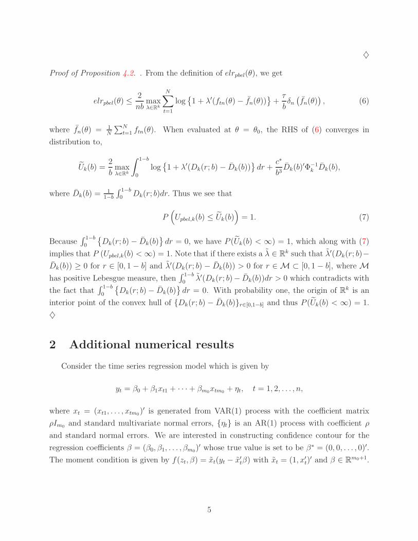
Proof of Proposition 4.2. . From the definition of elrpbel(θ), we get

elrpbel(θ) ≤2

nbmaxλ∈Rk

N∑

t=1

log{1 + λ′(ftn(θ)− fn(θ))

}+

τ

bδn

(fn(θ)

), (6)

where fn(θ) = 1N

∑N

t=1 ftn(θ). When evaluated at θ = θ0, the RHS of (6) converges in

distribution to,

Uk(b) =2

bmaxλ∈Rk

∫ 1−b

0

log{1 + λ′(Dk(r; b)− Dk(b))

}dr +

c∗

b3Dk(b)

′Φ−1k Dk(b),

where Dk(b) =1

1−b

∫ 1−b

0Dk(r; b)dr. Thus we see that

P(Upbel,k(b) ≤ Uk(b)

)= 1. (7)

Because∫ 1−b

0

{Dk(r; b)− Dk(b)

}dr = 0, we have P (Uk(b) < ∞) = 1, which along with (7)

implies that P (Upbel,k(b) < ∞) = 1. Note that if there exists a λ ∈ Rk such that λ′(Dk(r; b)−

Dk(b)) ≥ 0 for r ∈ [0, 1 − b] and λ′(Dk(r; b) − Dk(b)) > 0 for r ∈ M ⊂ [0, 1 − b], where Mhas positive Lebesgue measure, then

∫ 1−b

0λ′(Dk(r; b)− Dk(b))dr > 0 which contradicts with

the fact that∫ 1−b

0

{Dk(r; b)− Dk(b)

}dr = 0. With probability one, the origin of Rk is an

interior point of the convex hull of {Dk(r; b) − Dk(b)}r∈[0,1−b] and thus P (Uk(b) < ∞) = 1.

♦

2 Additional numerical results

Consider the time series regression model which is given by

yt = β0 + β1xt1 + · · ·+ βm0xtm0

+ ηt, t = 1, 2, . . . , n,

where xt = (xt1, . . . , xtm0)′ is generated from VAR(1) process with the coefficient matrix

ρIm0and standard multivariate normal errors, {ηt} is an AR(1) process with coefficient ρ

and standard normal errors. We are interested in constructing confidence contour for the

regression coefficients β = (β0, β1, . . . , βm0)′ whose true value is set to be β∗ = (0, 0, . . . , 0)′.

The moment condition is given by f(zt, β) = xt(yt − x′tβ) with xt = (1, x′

t)′ and β ∈ R

m0+1.

5

To implement the penalized methods, we consider the self-normalization matrix

Ψn(θn) =1

n

n∑

i=1

n∑

j=1

(1−

∣∣∣∣i− j

n

∣∣∣∣)f(zi, βn)f(zj , βn)

′,

with βn being the least square estimate. We set ρ = −0.5, 0.2, 0.5, 0.8, and m0 = 1, 4.

Figures 1-2 present respectively the coverage probabilities for PBEL and PEBEL, and their

unpenalized counterparts at the 95% nominal level. Note that for m0 = 4, we only present

the results for the penalized methods as the unpenalized counterparts severely suffer from

the coverage upper bound problem. Overall, the results are qualitatively similar to those for

the mean case. When m0 = 1 (i.e. k = 2), the PBEL provides better coverage uniformly

over b as compared to the BEL when ρ = 0.5 and 0.8. The improvement becomes more

significant as the block size grows. When m0 = 4 (i.e. k = 5), we note that the choice of c∗

that delivers the most accurate coverage is delicate as it depends on b and the strength of

dependence. For PEBEL, the improvement on the coverage probabilities is again significant

for the range of c∗ being considered. When m0 = 4, the coverage probability is sensitive to

the choice of c∗ and we expect the block bootstrap method described in Section 5.2 to be

useful in this case.

3 Fixed-b asymptotics versus small-b asymptotics

For the coverage upper bound problem, the fixed-b method is more appropriate than the

small-b method in terms of describing the finite sample situation because one cause of the

coverage upper bound problem in the dependent case is the choice of the blocking strategy

and block size which is explicitly reflected in the fixed-b limit. For instance, when the finite

sample bound problem occurs, the fixed-b method correctly reflects such a phenomenon in

the asymptotics, while the original BEL under the small-b asymptotics is somewhat “over-

optimistic” as the corresponding upper bound in the limit is always one regardless of what

the finite sample bound is.

The basic philosophy behind the fixed-b method is to embed the finite sample situation

in a different limiting thought experiment, where b (the fraction of block size relative to

sample size) is held fixed as the sample size grows. In the small-b asymptotics, b goes

to zero as sample size n → +∞, which is a convenient assumption for deriving a limiting

distribution. However, as pointed out in Kiefer and Vogelsang (2005) [also see Neave (1970)],

this assumption can be unrealistic when the deduced results are used as approximations to

the finite sample case where the value of b can never be zero. Thus, the finite sample coverage

6

upper bound problem in general does not go away since b cannot be zero. The usefulness

of the fixed-b approach has been demonstrated in many other contexts; see Sun (2013);

Kiefer and Vogelsang (2005); Shao (2010), Shao and Politis (2013), among others. Using the

higher-order Edgeworth expansions, Jansson (2004), Sun et al. (2008), Sun (2014) and Zhang

and Shao (2013) rigorously proved that the fixed-b type asymptotics provides a high order

refinement over the traditional small-b type asymptotics in the Gaussian location model. It

is also worth pointing out that the fixed-b method and small-b method are consistent for

relatively small b in the BEL context [see e.g. Remark 2 of Zhang and Shao (2014)]. Given

the connection between BEL and generalized method of moments framework, for which

the fixed-b approach has been successfully extended to [see Kiefer and Vogelsang (2005),

Vogelsang (2003)], we believe that the nice properties of fixed-b approach as found in other

contexts carry over to the BEL case, which has been partially confirmed in Zhang and Shao

(2014).

The fixed-b asymptotics not only provides better approximation for the original BEL

but it also tends to provide better approximation for the penalized counterpart. To further

illustrate the superiority of the fixed-b approach over the small-b approach in the PBEL

context, we shall present some simulation results. Following the setup in Section 5, we

focus on the confidence region for the mean of univariate/multivariate time series. In the

univariate case, we consider the AR(1) process zt = ρzt−1 + εt with ρ = −0.5, 0.2, 0.5, 0.8,

where {εt} is a sequence of i.i.d standard normal errors. In the multidimensional case (i.e.

k > 1), we generate multivariate time series with each component being independent AR(1)

process. The sample size n = 100 and the nominal level is 95%. To construct confidence

interval for the mean of the time series, we consider the BEL and PBEL under both fixed-b

and small-b asymptotics. Recall the definition of the PBEL ratio test statistic which is given

by,

elrpbel(θ) = minµ∈Rk

{2

nbmaxλ∈Rk

N∑

t=1

log {1 + λ′(ftn(θ)− µ)}+ τ

bδn (µ)

}.

For PBEL under the small-b asymptotics, we shall use the critical value from χ2 distribution

to conduct inference. The χ2 approximation is only valid when b is small and c∗ is large

because for large c∗, the PBEL ratio statistic behaves like the BEL ratio statistic which has

a χ2 limit when b is small. Note that when c∗ is small, the penalty term dominates and the

limiting distribution is no longer χ2. Thus for relatively small c∗ (e.g. c∗ = 0.01), we do

not present the results for PBEL under the small-b asymptotics. Figure 3 plots the coverage

probabilities for the four methods: small-b based BEL, fixed-b based BEL, small-b based

PBEL and fixed-b based PBEL. Again, the fixed-b based methods significantly outperform

the small-b counterparts for relatively large b. We also observe that the penalized methods in

7

general provide improvement over the unpenalized counterparts. The improvement is quite

significant especially when c∗ is small and b is relatively large. Overall, this small simulation

illustrates the advantage of the fixed-b method and also demonstrates the usefulness of the

penalized method.

References

Jansson, M. (2004). On the error of rejection probability in simple autocorrelation robust

tests. Econometrica 72 937-946.

Kiefer, N. M. and Vogelsang, T. J. (2005). A new asymptotic theory for heteroskedasticity-

autocorrelation robust tests. Econometric Theory. 21 1130-1164.

Neave, H. R. (1970). An improved formula for the asymptotic variance of spectrum estimates.

Ann. Math. Statist. 41 70-77.

Shao, X. (2010). A self-normalized approach to confidence interval construction in time series.

J. R. Stat. Soc. Ser. B Stat. Methodol. 72 343-366.

Shao, X. and Politis, D. (2013). Fixed-b subsampling and block bootstrap: improved confi-

dence sets based on p-value calibration. J. R. Stat. Soc. Ser. B Stat. Methodol. 75 161-184.

Sun, Y., Phillips, P. C. B. and Jin, S. (2008). Optimal bandwidth selection in

heteroscedasicity-autocorrlation robust testing. Econometrica 76 175-194.

Sun, Y. (2013). Fixed-smoothing asymptotics in a two-step GMM framework. Working paper,

Department of Economics, UCSD.

Sun, Y. (2014). Let’s fix it: fixed-b asymptotics versus small-b asymptotics in heteroscedas-

ticity and autocorrelation robust inference. J. Econometrics 178 659-677.

Vogelsang, T. (2003). Testing in GMM Models Without Truncation Chapter 10 of Advances

in Econometrics Volume 17, Maximum Likelihood Estimation of Misspecified Models: Twen-

ty Years Later, ed. by T. B. Fomby and R. C. Hill, Elsevier Science, 199-233.

Zhang, X. and Shao, X. (2013). Fixed-smoothing asymptotics for time series. Ann. Statist.

41 1329-1349.

Zhang, X. and Shao, X. (2014). Fixed-b asymptotics for blockwise empirical likelihood. S-

tatist. Sinica 24 1179-1194.

8

0.05 0.10 0.15 0.20

8085

9095

100

AR(1), rho=0.2

b

cove

rage

per

cent

age

PBEL−Fb, c*=0.01, 100PBEL−Fb, c*=0.01, 400PBEL−Fb, c*=2, 100PBEL−Fb, c*=2, 400BEL−Fb, 100BEL−Fb, 400

80

85

90

95

10

0

AR(1), rho=0.2

c*

cove

rag

e p

erc

en

tag

e

0.001 0.01 0.05 0.1 0.2 0.4 0.6 0.8 1 2

PBEL−Fb, b=0.05, 100PBEL−Fb, b=0.05, 400PBEL−Fb, b=0.1, 100PBEL−Fb, b=0.1, 400

0.05 0.10 0.15 0.20

8085

9095

100

AR(1), rho=0.5

b

cove

rage

per

cent

age


65

70

75

80

85

90

95

AR(1), rho=0.5

c*

cove

rag

e p

erc

en

tag

e

0.001 0.01 0.05 0.1 0.2 0.4 0.6 0.8 1 2


0.05 0.10 0.15 0.20

5060

7080

9010

0

AR(1), rho=0.8

b

cove

rage

per

cent

age


40

50

60

70

80

90

10

0

AR(1), rho=0.8

c*

cove

rag

e p

erc

en

tag

e

0.001 0.01 0.05 0.1 0.2 0.4 0.6 0.8 1 2


0.05 0.10 0.15 0.20

8688

9092

9496

98

AR(1), rho=−0.5

b

cove

rage

per

cent

age


85

90

95

10

0

AR(1), rho=−0.5

c*

cove

rag

e p

erc

en

tag

e

0.001 0.01 0.05 0.1 0.2 0.4 0.6 0.8 1 2


Figure 1: Coverage probabilities for the regression coefficients delivered by the PBEL withQ(r, s) = (1−|r− s|)I{|r− s| ≤ 1}, and BEL, where m0 = 1 for the left column and m0 = 4for the right column. The nominal level is 95% and the number of Monte Carlo replicationsis 1,000.

9

60

70

80

90

10

0

AR(1), rho=0.2

c*

cove

rag

e p

erc

en

tag

e

0.001 0.01 0.05 0.1 0.2 0.4 0.6 0.8 1 2

PEBEL−Fb, 100PEBEL−Fb, 400EBEL−Fb, 100EBEL−Fb, 400

75

80

85

90

95

10

0

AR(1), rho=0.2

c*

cove

rag

e p

erc

en

tag

e

0.001 0.01 0.05 0.1 0.2 0.4 0.6 0.8 1 2

PEBEL−Fb, 100PEBEL−Fb, 400

60

70

80

90

10

0

AR(1), rho=0.5

c*

cove

rag

e p

erc

en

tag

e

0.001 0.01 0.05 0.1 0.2 0.4 0.6 0.8 1 2


70

75

80

85

90

95

10

0

AR(1), rho=0.5

c*

cove

rag

e p

erc

en

tag

e

0.001 0.01 0.05 0.1 0.2 0.4 0.6 0.8 1 2


50

60

70

80

90

10

0

AR(1), rho=0.8

c*

cove

rag

e p

erc

en

tag

e

0.001 0.01 0.05 0.1 0.2 0.4 0.6 0.8 1 2


50

60

70

80

90

10

0

AR(1), rho=0.8

c*

cove

rag

e p

erc

en

tag

e

0.001 0.01 0.05 0.1 0.2 0.4 0.6 0.8 1 2


65

70

75

80

85

90

95

AR(1), rho=−0.5

c*

cove

rag

e p

erc

en

tag

e

0.001 0.01 0.05 0.1 0.2 0.4 0.6 0.8 1 2


70

75

80

85

90

95

10

0

AR(1), rho=−0.5

c*

cove

rag

e p

erc

en

tag

e

0.001 0.01 0.05 0.1 0.2 0.4 0.6 0.8 1 2


Figure 2: Coverage probabilities for the regression coefficients delivered by the PEBEL withvarious c∗ and Q(r, s) = (1 − |r − s|)I{|r − s| ≤ 1}, and EBEL, where m0 = 1 for the leftcolumn and m0 = 4 for the right column. The nominal level is 95% and the number ofMonte Carlo replications is 1,000.

10

0.05 0.15 0.25 0.35

6570

7580

8590

95

AR(1), rho=0.2

b

cove

rage

per

cent

age

PBEL−Fb,c*=0.01PBEL−Fb,c*=1PBEL−Sb,c*=1BEL−FbBEL−Sb

0.05 0.10 0.15 0.20

4050

6070

8090

100

AR(1), rho=0.2

b

cove

rage

per

cent

age


0.05 0.15 0.25 0.35

6070

8090

100

AR(1), rho=0.5

b

cove

rage

per

cent

age


0.05 0.10 0.15 0.20

2040

6080

100

AR(1), rho=0.5

b

cove

rage

per

cent

age


0.05 0.15 0.25 0.35

4050

6070

8090

100

AR(1), rho=0.8

b

cove

rage

per

cent

age


0.05 0.10 0.15 0.20

020

4060

8010

0

AR(1), rho=0.8

b

cove

rage

per

cent

age


0.05 0.15 0.25 0.35

7075

8085

9095

100

AR(1), rho=−0.5

b

cove

rage

per

cent

age


0.05 0.10 0.15 0.20

6070

8090

100

AR(1), rho=−0.5

b

cove

rage

per

cent

age


Figure 3: Coverage probabilities for the mean delivered by the PBEL with Q(r, s) = (1 −|r− s|)I{|r− s| ≤ 1}, and BEL under both small-b and fixed-b asymptotics, where k = 1 forthe left column and k = 2 for the right column. The nominal level is 95% and the numberof Monte Carlo replications is 1,000.

11

Table 1: 95% quantiles of the limiting distributions for BEL (uel,k(b; 1−α)) and PBEL (withthe Bartlett kernel) under the fixed-b asymptotics

BEL PBEL, c∗ = 0.01 PBEL, c∗ = 0.2 PBEL, c∗ = 2

b k = 1 k = 2 k = 1 k = 2 k = 1 k = 2 k = 1 k = 2

0.02 3.96 6.10 2.58 4.44 3.83 6.03 3.94 6.160.04 4.07 6.45 2.11 3.89 3.76 6.06 3.99 6.340.06 4.29 6.84 1.83 3.46 3.77 6.26 4.09 6.600.08 4.46 7.37 1.61 3.19 3.77 6.50 4.16 6.960.10 4.76 7.89 1.43 3.01 3.86 6.77 4.34 7.400.12 5.18 8.63 1.29 2.79 3.94 7.14 4.43 7.890.14 5.44 9.49 1.18 2.62 3.98 7.49 4.52 8.460.16 5.91 10.49 1.10 2.54 4.03 7.85 4.64 9.280.18 6.29 11.91 1.03 2.50 4.23 8.38 4.95 10.290.20 6.72 13.42 0.95 2.43 4.22 8.90 5.09 11.550.22 7.27 16.53 0.90 2.36 4.23 9.36 5.29 13.380.24 7.76 24.09 0.85 2.62 4.34 10.82 5.61 18.430.26 8.69 Inf 0.81 2.70 4.41 10.99 6.07 24.080.28 9.83 Inf 0.77 2.75 4.50 11.52 6.51 33.170.30 11.40 Inf 0.73 2.56 4.61 11.66 6.86 80.270.32 13.54 Inf 0.70 2.72 4.68 14.63 7.74 73.310.34 21.11 Inf 0.68 2.81 4.68 23.04 8.23 67.06

Table 2: 95% quantiles of the limiting distributions for PEBEL (with the Bartlett kernel)

c∗

k = 1 k = 2

0.001 0.007 0.0130.010 0.063 0.1200.050 0.264 0.4530.100 0.445 0.7090.200 0.684 1.0110.400 0.943 1.3710.600 1.105 1.6220.800 1.217 1.7581.000 1.303 1.9022.000 1.577 2.413

12

On the coverage bound problem of empirical likelihood ...zhangxiany/CB-2015.pdf · 2 X.Zhang and...

Documents

Transcript of On the coverage bound problem of empirical likelihood ...zhangxiany/CB-2015.pdf · 2 X.Zhang and...