On the Convergence of Recursive Trust-Region Methods for...

On the Convergence of Recursive Trust-Region Methods for Multiscale Non-Linear Optimization

and Applications to Non-Linear Mechanics

Christian Groß, Rolf Krause

no. 389

Diese Arbeit ist mit Unterstützung des von der Deutschen Forschungs-

gemeinschaft getragenen Sonderforschungsbereichs 611 an der Universität

Bonn entstanden und als Manuskript vervielfältigt worden.

Bonn, März 2008

ON THE CONVERGENCE OF RECURSIVE TRUST–REGIONMETHODS FOR MULTISCALE NON–LINEAR OPTIMIZATION

AND APPLICATIONS TO NON–LINEAR MECHANICS

CHRISTIAN GROSS∗ AND ROLF KRAUSE†

Abstract. We prove new convergence results for a class of multiscale trust–region algorithmsintroduced by Gratton et al. in [GST06] to solve unconstrained minimization problems withinthe Euclidean space Rn. We will state less restrictive assumptions on the function which has to beminimized and on the iteratively computed trust–region corrections, which allow for proving first– andsecond–order convergence and, moreover, locally quadratic convergence. We show the efficiency androbustness of our approach by means of examples from nonlinear continuum mechanics. Numericalresults in 3d for Ogden materials are presented.

Key words. nonlinear programming, nonlinear multilevel methods, nonlinear elasticity, con-vergence theory

AMS subject classifications. 65N55 65K05 35J60 90C26 90C30

1. Introduction. Often, the numerical solution of physical, biological and chem-ical problems gives rise to the solution of non-convex minimization problems. Forinstance, the deformation of soft tissue leads to a non-convex minimization problem,which is connected to a partial differential equation. As the capability of computersproceeds more and more, the solution of large scale non-linear sparse systems arisingfrom the discretization of partial differential equations becomes possible. As a con-sequence, also the development of efficient and reliable methods for such large andnon-convex minimization problems has become an active area of research over thepast decades [CL94, CGT00, GST06].

In this work, we consider the finite-dimensional and non-convex minimizationproblem

u ∈ Rn : J(u) = min! (M)

where J : Rn → R is at least continuously differentiable. But, J is neither assumedto be quadratic nor convex. As a consequence, we will only aim at the computationof a local minimizer u of J .

Several classes of methods to solve non-convex minimization problems emergedover the last decades, for instance, damped Newton methods (as an introduction see[Deu04]), trust–region algorithms (see, e.g., [CGT00]) or the Levenberg-Marquandtmethod [Lev44, Mar63, Mor78] as a special case of trust–region methods. Withinthese methods corrections are iteratively computed to yield a solution of problem(M). In addition, these strategies employ numerically applicable quality controls ofthe approximately computed corrections. Under certain conditions convergence tofirst- and second-order critical points for problem (M) can be proven (see, e.g., [CL94,UUH99]).

∗Institute for Numerical Simulation, University of Bonn. The research of this author was sup-ported by the Hausdorff Center for Mathematics, the Bonn International Graduate School and theDFG – “SFB 611 Singular Phenomena and Scaling in Mathematical Models”, [email protected]

†Institute for Numerical Simulation, University of Bonn. The research of this author was sup-ported by the DFG – “SFB 611 Singular Phenomena and Scaling in Mathematical Models” andHausdorff Center for Mathematics, [email protected]

1

2 C. GROSS and R. KRAUSE

The trust–region paradigm is to solve a constrained quadratic minimization prob-lem to obtain an energy reducing correction for problem (M). Numerically, the ma-jor draw-back of the disposition of these quadratic functions, as for the solution ofhighly non-linear problems in general, is the need to repeatedly compute gradientsand Hessians of the function J . In many applications, this requires a computationallyexpensive quadrature. Even worse, the naive application of such Newton-like strate-gies to solve large scale non-convex minimization problems tends to be inefficient aslong as the region of superlinear convergence is not yet reached. A possible solutionis to use state of the art direct solution strategies for linear systems in combinationwith active set strategies to solve the linear systems of equations to compute a correc-tion [LHKK79, SG04, WB06]. In case of convex constrained subproblems monotonemultigrid methods can be used [KKS+06, Kor97]. In this work we will follow anotherapproach, more precise, a generalized multilevel ansatz.

Multiscale or multilevel methods have been extensively analyzed for quadraticminimization problems, e.g., for the solution of linear elliptic partial differential equa-tions. By using a sequence of generally nested subspaces (geometric) multilevel meth-ods have been proven to provide the sought-after solution with optimal complex-ity [BPS86, Bra93, Osw94, TE98, Bad06]. Multilevel methods, however, have beendesigned for linear and symmetric positive definite systems, as arise as first ordersystem for (strictly convex) quadratic minimization problems. Nevertheless, gener-alized multilevel algorithms were developed to solve highly non-linear minimizationproblems, like FAS [Bra81] and MG/OPT [Nas00, LN05].

In contrast to linear multilevel methods, coarse level corrections in FAS andMG/OPT are computed based on non-linear coarse level representations of J . In[GST06], the use of a trust–region strategy was proposed to solve the occurring mini-mization problems which yields a restrained MG/OPT version called RMTR (Recur-sive Multilevel Trust–Region Method).

In [GST06] it is shown, that the RMTR algorithm generates a sequence of iter-ates converging to first–order critical points if the function J is twice continuouslydifferentiable. In the present work, we will show that for a V-cycle version of theRMTR algorithm first–order convergence can be achieved even if J is just continu-ously differentiable. Moreover, we state additional assumptions, in particular J ∈ C2,and, hence, are able to show convergence to second–order critical points, as well aslocally quadratic converge. Moreover, we render a reasonable choice of initial coarselevel iterates and illustrate differences to [GST06]. Finally, we show the robustnessand efficiency of our implementation by presenting different examples arising fromthe field of elasticity in 3d and present a comparison of the numerical behavior ofdifferent trust–region algorithms, i.e., the RMTR, cascadic multigrids, RMTR withnested iteration and a “single–level” trust–region algorithm.

This paper will be organized as follows. In Section 2 we will introduce our mul-tilevel framework, characterize and introduce the used interpolation, restriction andprojection operator, as well as define a generally non-linear coarse level model, whichis minimized to obtain a coarse level correction. In Section 3 we introduce the trust–region algorithm which is applied to compute those corrections on each level. TheRMTR algorithm which merges the local trust–region strategies to a V-cycle algorithmis introduced in Section 4. In this section we then prove local quadratic convergenceto first- and second order critical points. In Section 5 we report on linear and non-linear examples taken from the area of elasticity. In particular, we compute threedimensional boundary value problems for bodies which suffice linear elastic material

On the Convergence and Applications of Recursive Trust–Region Methods 3

Fig. 2.1. A scheme of the employed V-cycle algorithm

laws (see [Cia88]) and Ogden-like material laws (see [Ogd97]).

2. A Multilevel Setting. Multiresolution algorithms which are designed tosolve quadratic minimization problems in function spaces tend to be efficient dueto their ability to resolve different spectra on different levels (cf. [Dah97, BPS86,Osw94]). Commonly used for solving quadratic minimization problems associated toelliptic PDEs are multigrid methods (as an introduction see, e.g., [Bra07]). Thesemethods employ a sequence of (nested) subspaces, associated to each other by inter-polation and restriction operators. The linear residual of the quadratic function, i.e.,the first-order sufficiency condition, is restricted to coarser levels and used to computeso-called coarse level corrections which are in turn interpolated to the finer level.

However, since our minimization problem is in general highly non-linear the first-order sufficiency conditions are also non-linear. Hence, in our case a different approachmust be chosen: We define level-dependent non-convex functions (see section 2.4),which are utilized to compute coarse level corrections. Due to the non-convexity ofthese functions a trust–region strategy is employed to compute these corrections. Inthe end, the resulting multilevel strategy is designed as a V-cycle version of the RMTRalgorithm, presented in [GST06].

In the following, we describe the multilevel setting used for our RMTR-methodin a matrix based notation. In the ν-th cycle and on the k-th level, the algorithmcomputes m1 ≥ 0 corrections to minimize the level dependent function, denoted byHν

k , yielding an intermediate iterate. In our framework, this reduction of the Hνk

values is carried out using a trust–region strategy. The computation of these m1

trust–region steps yields a new iterate, where one trust–region step is an approximatesolution of a quadratic minimization problem. The m1-st iterate is employed togenerate the coarse level function on the next coarser level, level k − 1. Moreover,the projection of this iterate is the initial iterate on level k − 1. A computation onthis level yields a coarse level correction, which will be transferred to level k andthere accepted or discarded as coarse level correction. Afterwards another m2 ≥ 0corrections are computed using the trust–region strategy. Finally, the interpolateddifference between first and last iterate on level k is the coarse level correction onlevel k+ 1. On the coarsest level, indeed, will no recursion be called. If k is the finestlevel, denoted by the index j, the last iterate on this level will be defined as the firstiterate in the next cycle, cycle ν+1. The coarsest level in cycle ν, i.e., the level whereno recursion is called, will be denoted by kν . Summarized this yields figure 2.1.

2.1. The Multilevel Decomposition. We will now decompose the space Rn,where problem (M) is posed, into a sequence of nested subspaces beginning at the


finest level j ≥ 0. This decomposition depends on the number ν of already performedV-cycles. Hence, in each cycle the linear space Rn is decomposed into kν subspaces,i.e.,

Rn = Rnj ) Rnνj−1 ) · · · ) Rnν

kν (2.1)

Moreover, we assume without loss of generality that kν ≥ 0 for all ν ≥ 0. TheEuclidean spaces Rnν

k provide the inner product 〈·, ·〉 and the norm ‖u‖22 = 〈u, u〉. In

the remainder, the subspaces will be indexed by k, i.e., j ≥ k ≥ kν .The spaces Rnν

k are linked to each other by linear restriction and interpolationoperators. The restriction operator is Rk,ν

k+1 : Rnνk+1 → Rnν

k and the interpolation

operators satisfy Ik+1,νk : Rnν

k → Rnνk+1 for kν ≤ k < j. We assume that the relation

holds:

Ik+1,νk = (Rk,ν

k+1)T

A more general assumptions on the restriction and interpolation is often used(see, e.g., [Nas00, GST06]). It is assumed that a scalar σν

k > 0 exists such that

Ik+1,νk = σν

k (Rk,νk+1)

T . However, our results in Section 4.3 and 4.4 hold the same waywith σν

k ≥ 1. The choice of σνk 6= 1 only influences the result and proof of Theorem

4.6. Furthermore, we assume that the interpolation and restriction operators willhave the following properties.

(I) The operators Ik+1,νk : Rnν

k → Rnνk+1 are assumed to have full rank and it is

assumed that the smallest eigenvalue λmin and the largest eigenvalue λmax of(Ik+1,ν

k )T Ik+1,νk are bounded away from zero and infinity, respectively. That

is, for all ν ≥ 0 and on all levels k ∈ kν, . . . , j − 1 there exist constantscR, CI ≥ cI > 0 such that

λmin((Ik+1,νk )T I

k+1,νk ) ≥ cI

λmax((Ik+1,νk )T I

k+1,νk ) ≤ CI

cR ≥ ‖Rk,νk+1‖2

Finally it is assumed that Rk,νk+1 = (Ik+1,ν

k )T .

2.2. Introduction of the Iterates and Corrections. As pointed out before,the algorithm proposed in this work is the combination of a multilevel and a trust–region strategy. We employ the trust–region strategy as a smoother to computelocal corrections, i.e., non-recursively computed corrections. Hence, on each level weperform m1 ∈ N smoothing steps before calling a recursion and m2 ∈ N afterwards. Inbetween, the current iterate on the current level is restricted to the next coarser gridwhere, in turn, a correction is computed by means of the trust–region strategy anda possible further recursion. The resulting coarse level correction, i.e., the differencebetween initial and last iterate on the next coarser level, is interpolated to the currentlevel yielding a recursively computed correction. Alltogether, this constitutes a non-linear V-cycle algorithm.

The number of already performed V-cycles will be indexed by ν ∈ N and weassume that the initial iterate on the finest grid, i.e., u0

j,0 ∈ Rn, is given a priori.Moreover, it is reasonable to assume that at least m1 or m2, i.e., the number ofsmoothing steps, is not zero. The integer mν

k denotes the number of computed cor-rections on Level k in Cycle ν. Corrections sk,i, i 6= m1, computed by means of the


Fig. 2.2. Current fine level iterate and resulting L2-projected and restricted iterates

trust–region strategy, will be called trust–region corrections and their computationtrust–region steps.

As pointed out before, a recursively computed correction is the m1-st correctionon level k and the interpolated difference of the initial and last iterate on level k − 1,i.e., sk,m1 = I

k,νk−1(u

νk−1,mν

k−1− uν

k−1,0)for k > kν . Since the quality of corrections

is controlled, it turns out that not all corrections are applied. But, if sk,i is ratedto be a sufficiently good correction, we define the next iterate as uν

k,i = uνk,i + sk,i

for i = 0, . . . ,mνk. However, even if a correction is not applied, the index i will be

incremented. We will see that only if the norm of the gradient of Hνk is sufficiently

small or if the maximal number of iterations is exceeded, the computation on level kterminates.

2.3. A novel Projection Approach. As a matter of fact, the restriction oper-ator in standard linear multigrid methods (see for example [Bra07, Kor97, GO95]) isdesigned as a dual operator, i.e., to restrict the linear defect to a coarser level. Hence,this operator is not designed to project a primal variable, i.e., the iterate, to coarselevels. In our approach, we therefore introduce the additional projection operatorP

k−1,νk : Rnν

k → Rnνk−1 to transfer the primal variable. Hence, we define the initial

coarse level iterate on level k − 1 as uνk−1,0 = P

k−1,νk uν

k,m1. However, the correction

vector as a primal variable will be interpolated using the operator Ik,νk−1. In Figure

2.2, we illustrate the difference between both operators.

2.4. Derivation of the Level-Dependent Models. In this section, we in-troduce level dependent functions, whose minimization can yield good coarse levelcorrections to finally solve (M). In the context of quadratic and strictly convex min-imization problems, such coarse level functions are based on the quadratic functionitself, the linear residual and on the restriction operator. Nash introduced in [Nas00]a concept aimed on non-linear minimization problems, which reduces in the quadraticcontext to a linear multilevel algorithm.

Assume that for each ν ≥ 0 and all k ∈ j − 1, . . . , kν level-dependent andcontinuously differentiable functions Jν

k : Rnνk → R are given which approximate J on

level k. Moreover, we assume that Jνj = J holds on the finest level.

Now we define the level dependent and non-linear function Hνk : Rnν

k → R for all

ν ≥ 0 and all k ∈ j, . . . , kν as

Hνk (uk) = Jν

k (uk) + 〈δgνk , uk − uν

k,0〉 ∀uk ∈ Rnνk (2.2)

Here, the residual δgνk ∈ Rnν

k is given by

δgνk =

Rk,νk+1g

νk+1(u

νk+1,m1

) −∇Jνk (uν

k,0) if j > k ≥ kν

0 if k = j


where we use the abbreviations Hνk,i = Hν

k (uνk,i) for the local energy at uν

k,i andgν

k,i = ∇Hνk (uν

k,i) for the gradient. Further assumptions on Hνk and the gradients gν

k,i

are formulated in section 3.1.

3. A Trust–Region Algorithm. The minimization of arbitrary non-convexfunctions as the coarse-level functions Hν

k from (2.2), is a demanding task. For ex-ample, for Newton’s method local convergence can only be guaranteed, if the initialiterate is sufficiently close to a local minimizer. In order to obtain a convergentmethod, we employ a trust–region algorithm as a globalization strategy (see, e.g.,[GST06, CL94, UUH99]).

The trust–region paradigm is to use, on the one hand, Newton’s method and,on the other hand, to control the quality of the computed corrections. Therefore, atrust–region solver iteratively computes corrections, by means of a so-called trust–region model, which is a second order Taylor approximation of the function Hν

k . Thecomputed corrections are required to stay in a ”trust–region” with radius ∆. Thisradius ∆ varies depending on the so-called contraction rate which is the relation be-tween the – by the trust–region model – predicted reduction and the actual reductionwhich is measured in terms of Hν

k . However, a second order approximation requiresthe computation of the Hessian of Hν

k , which, in turn, requires sufficient smoothnessof Jν

k , as well as computation time. Even worse: Numerically, the computation of theHessian may suffer from a lack of computational accuracy leading to poor approxi-mations of ∇2Hν

k (uνk,i). Hence, one approximates the Hessians ∇2Hν

k (uνk,i) by means

of a symmetric matrix Bνk,i.

In the end, a trust–region step, i.e., the computation of a correction and itsevaluation, depends on the current trust–region model, the solution of a constrainedminimization problem, an evaluation of the correction’s quality and the adjustmentof the trust–region radius. The combination of these steps yields Algorithm 1 on page8. We will now explain these four steps in detail.

3.1. Assumptions on Hνk and the Trust–Region Model. In this section,

we derive the trust–region model ψνk,i as a quadratic approximation of Hν

k,i(uνk,i + ·).

To this end, we make the following assumptions in addition to (I).(A1) For the given initial iterate u0

j,0 ∈ Rnj , for all ν ≥ 0 and all levels k ∈kν , . . . , j − 1 and all initial coarse grid iterates uν

k,0 ∈ Rnνk , it is assumed

that the level sets

Lνk = u ∈ Rnν

k | Hνk (u) ≤ Hν

k (uνk,0)

and

L0j = u ∈ Rnj | Jj(u) ≤ Jj(u

0j,0)

are compact.(A2) For all ν ≥ 0 and all levels k ∈ kν , . . . , j we assume that Hν

k is continuouslydifferentiable on Lν

k. Moreover, we assume that there exists a constant cg > 0such that for all iterates uν

k,i ∈ Lνk holds ‖gν

k,i‖2 = ‖∇Hνk (uν

k,i)‖2 ≤ cg.

(A3) For all ν ≥ 0 and all levels k ∈ kν , . . . , j there exists a constant cB > 0 suchthat for all iterates uν

k,i ∈ Lνk and the employed symmetric approximationBν

k,i

of ∇2Hνk (uν

k,i) the inequality ‖Bνk,i‖2 ≤ cB is satisfied.

Now, for given uνk,i the trust–region model is given as ψν

k,i : Rnνk → R with

ψνk,i(s) = Jν

k (uνk,i) + 〈gν

k,i, s〉 +1

2〈s,Bν

k,is〉 (3.1)


3.2. Computing Corrections. Employing the trust–region model ψνk,i, a cor-

rection sk,i ∈ Rnνk is computed as an approximate solution of the constrained mini-

mization problem

mins∈R

nνk

ψνk,i(u

νk,i + s), s.t. ‖s‖kν ≤ ∆ν

k,i (3.2)

where ∆νk,i ∈ R+ is the trust–region radius. We emphasize that the trust–region strat-

egy allows also for approximately solving (3.1), which avoids its possibly expensiveexact solution.

3.3. Contraction Rates and Trust–Region Update. Since, on the one handsk,i is computed approximately and on the other hand Hν

k is arbitrarily non-linear,one has to control the quality of sk,i. Hence, we define the actual and the predictedreduction as

aredνk,i(s) = Hν

k (uνk,i) −Hν

k (uνk,i + s)

predνk,i(s) = −〈s, gν

k,i〉 −1

2〈s,Bν

k,is〉

In fact, predνk,i(s) measures Hν

k (uνk,i)−Hν

k (uνk,i + s) employing a second order Taylor

approximation of Hνk (uν

k,i + s).Finally, the correction sk,i is rated employing a scalar value, the contraction rate

ρνk,i. This scalar compares the actual reduction with the predicted one, i.e.,

ρνk,i =

aredνk,i(sk,i)

predνk,i(sk,i)

if predνk,i(sk,i) 6= 0

0 otherwise(3.3)

The trust–region update consists of two steps. First, the radius ∆νk,i is increased or

decreased depending on ρνk,i yielding an intermediate radius ∆ν

k,i. Since we sojournwithin the multilevel framework the trust–region update will finally depend also onDeltaν

k+1, the radius of the next finer level when calling the recursion. This meansthat the intermediate radius is shortend if it exceeds the radius of the finer level.

The intermediate radius is computed as

∆νk,i ∈

[∆νk,i, γ3∆

νk,i] if ρν

k,i ≥ η2

[γ2∆νk,i,∆

νk,i) if η1 ≤ ρν

k,i < η2

[γ1∆νk,i, γ2∆

νk,i) if ρν

k,i < η1

(3.4)

where 1 > η2 ≥ η1 > 0, as well as γ3 > 1 ≥ γ2 > γ1 > 0 are assumed to be given apriori and fixed for the whole computation. The new radius depends on the norm

‖uνk,i‖k,ν = ‖Ij,ν

j−1 · · · Ik+1,νk uν

k,i‖2

for k < j and ‖uνj,i‖j = ‖uν

j,i‖2 Now, the new trust region radius is

∆νk,i+1 = min∆ν

k,i,∆k+1 − ‖uνk,i+1 − uν

k,0‖k,ν (3.5)

where ∆k+1 is given a-priori, either as the fine-level radius ∆νk+1,m1

or, on the finestlevel, as ∆j+1 = ∞. This formulation ensures that the interpolated coarse level cor-rection will stay within the trust–region radius on the next finer grid.


If ρνk,i ≥ η1 holds, a correction is applied. Otherwise, the correction will be

rejected and the trust–region radius decreased. Note, that ρνk,i measures the curvature

of Hνk (uν

k,i) in direction of sk,i. For instance, if Hνk is a quadratic function in the

neighborhood of uνk,i, the contraction rate would be one.

Finally, these four steps are summarized in Algorithm 1. Within our version ofthe RMTR algorithm this trust-strategy is employed on each level to reduce Hν

k and,hence, to reduce Hν

j = J as well.

Algorithm: Local Trust–Region Solver

Input: nνk∈ N, uν

k,0, gνk,0 ∈ R

nνk ,∆ν

k,i∈ R, l ∈ N

Constants: γ1, γ2, γ3, η1, η2, εg,ν

k∈ R+

Output: new iterate uνk,i+1 ∈ R

nνk , trust–region radius ∆ν

k,i+1

if (‖gνk,0‖2 ≤ ε

g,νk

)

return uνk,0,∆

νk,0

for (i = 0, . . . , l− 1) generate ψν

k,iby means of (3.1)

solve problem (3.2) approximately and obtain sk,i ∈ Rnν

k

compute ρνk,i

according to (3.3)

if (ρνk,i

≥ η1)

uνk,i+1 = uν

k,i+ sk,i

else

uνk,i+1 = uν

k,i

if (‖gνk,i+1‖2 ≤ ε

g,ν

k) and (k 6= j)

return uνk,i+1

compute ∆νk,i+1 by means of (3.4)

return uνk,i+1,∆

νk,i+1

Algorithm 1: Local Trust–Region Algorithm

3.4. Sufficient Decrease Condition. To ensure convergence to first and sec-ond order critical points, problem (3.2) has to be solved sufficiently accurate. Hence,a commonly used criterion, the so-called Cauchy criterion, will now be introduced (cf.[CL94, UUH99]): We assume that a solution of (3.2) satisfies

φνk,i(sk,i) < βν

kφνk,i(s

Ck,i) w.r.t. ‖sk,i‖k,ν ≤ ∆ν

k,i (CC)

where

φνk,i(s) = 〈gν

k,i, s〉 +1

2〈s,Bν

k,is〉

and sCk,i ∈ Rnν

k solves

mins=−tgν

k,i|t≥0φν

k,i(s) w.r.t. ‖s‖k,ν ≤ ∆νk,i (3.6)

Furthermore, we assume that there exist constants β1, β2 ≥ 0 such that β1 ≥ βνk ≥

β0 > 0 for all ν ≥ 0 and all k ∈ kν, . . . , j.


Note, that the sufficient decrease condition (CC) can easily be checked by solvingthe scalar problem (3.6) exactly.

4. RMTR – Recursive Multilevel Trust–Region Method. As introducedby Gratton et al. [GST06], the RMTR algorithm, Algorithm 2, employs Algorithm1 to reduce Jj or to compute coarse level corrections. However, criteria (CC) andρν

k,i ≥ η1 take only effect on the reduction of Hνk . Hence, we introduce an additional

criterion, such that a coarse grid correction might be accepted or rejected, dependingon its effect on Hν

k+1.

4.1. Advancement Criteria in the Multilevel Context. To proof conver-gence to critical points, it is important being able to estimate the restricted coarselevel gradient by the fine level gradient. Hence, the RMTR algorithm will only proceedto a coarser level if

‖Rk−1,νk gν

k,m1‖2 ≥ κg‖gν

k,m1‖2 (AC)

holds where m1 is the index when calling the recursion and κg ∈ (0, 1).

Remark 4.1 Equation (AC) ensures additionally that a recursion will only be called

if the low-frequency contributions, Rk−1,νk gν

k,m1, of gν

k,m1are sufficiently large.

4.2. Acceptance Criteria in the Multilevel Context. In Section 2.2 wedefined the coarse level correction as

sk,m1 = Ik,νk−1(u

νk−1,mν

k−1− uν

k−1,0)

wheremνk−1 the index of the final iterate on level k−1. Now, we define the contraction

rate induced by such a correction sk,m1 as

ρνk,m1

=

Hνk (uν

k,m1)−Hν

k (uνk,m1

+sk,m1)

Hνk−1(uν

k−1,0)−Hνk−1(uν

k−1,mνk−1

) if uνk−1,0 6= uν

k−1,mνk−1

0 otherwise(4.1)

Hence, ρνk,m1

compares the effects of this correction on the coarse level function andthe fine level function. This quantity is used to accept or reject a coarse level correctionand to adjust the trust–region radius: The correction sk,m1 will only be accepted, if

ρνk,m1

≥ η1 (4.2)

holds. Finally, the trust–region radius update is carried out by substituting ρνk,m1

forρν

k,i in equation (3.5). Combining with Algorithm 1 yields Algorithm 2, the RMTRalgorithm, on page 10.

4.3. Convergence to First-Order Critical Points. Our convergence proofshave the following structure: We will show that if ρν

k,i ≥ η1 and if sk,i satisfies theCauchy decrease condition (CC), the difference Hν

k (uνk,i)−Hν

k (uνk,i + sk,i) is bounded

away from zero by a constant depending on ‖gνk,i‖2 and ∆ν

k,i. We emphasize thatthe functions Jν

k are not required to be twice continuously differentiable to obtainconvergence to first-order critical points. We point out that the occurring constantsc are generic and independent of ν, k, i.

We cite the result of Lemma 4.1 in [GST06], i.e., in our setup the coarse levelcorrections will not violate the fine level trust–region constraint.


Algorithm: RMTR

Input: nνk∈ N, uν

k,0, Rk,ν

k+1gνk+1,m1

∈ Rnν

k ,∆k+1 ∈ R+

Constants: γ1, γ2, γ3, η1, η2,

Output: new iterate uνk,mν

k∈ R

nνk for k < j

compute Hνk

as defined in (2.2)set ∆ν

k,0 = ∆k+1

Trust–Region Solver – Pre-Smoothingcall Algorithm 1 (see page 8) and receive a new iterate uν

k,m1

and a new trust–region radius ∆νk,m1

Recursion

compute nνk−1, Rk−1,ν

k, P k−1,ν

k

if (k > kν) and ((AC) holds)

call RMTR(nνk−1, P

k−1,νk

uνk,m1

| z

=uνk−1,0

, Rk−1,νk

gνk,m1

,∆νk,m1

| z

=∆k

) and receive uνk−1,mν

k−1

set sk,m1= I

k,ν

k−1(uνk−1,mν

k−1− uν

k−1,0)

compute ρνk,m1

by means of (4.1)

if ( ρνk,m1

≥ η1)

uνk,m1+1 = uν

k,m1+ sk,m1

else

uνk,m1+1 = uν

k,m1

update ∆νk,m1

according to (3.4)

Trust–Region Solver – Post-Smoothingcall Algorithm 1 (see page 8) and receive a new iterateand trust–region radius, i.e., uν

k,mνk,∆ν

k,mνk

if (k = j)

update ∆ν+1j,0 = ∆ν

j,m, uν+1j,0 = uν

j,mνj, ν = ν + 1

goto Trust–Region Solver – Pre-Smoothingelse

return uνk,mν

k

Algorithm 2: RMTR

Lemma 4.2 For all index triples (ν, k, i) and each sk,i ∈ Rnνk computed and accepted

in algorithm RMTR, it holds

‖sk,i‖k,ν ≤ ∆νk,i (4.3)

Moreover, for all k < j and 1 ≤ i ≤ mνk it holds

‖uνk,i − uν

k,0‖k,ν ≤ ∆νk+1,m1

(4.4)

In the spirit of Lemma 3.1, [CL94], the next result shows that the condition (CC)implies a certain decrease of φν

k,i and, hence, a reduction Hνk .


Lemma 4.3 Let assumptions (A1), (A2), (A3) and (I) hold. Then for all (ν, k, i)with uν

k,i ∈ Rnνk such that ∇Hν

k (uνk,i) = gν

k,i 6= 0 and all sk,i computed in Algorithm 1satisfying (CC) it holds

predνk,i(sk,i) ≥ cβ0‖gν

k,i‖22 min‖gν

k,i‖22,∆

νk,i (4.5)

where c > 0 is independent from (ν, k, i), only depends on CI from (I) and β0 from(CC).

Proof. Since the RMTR satisfies on each level the assumptions of Lemma 3.1,[CL94] we obtain using ‖u‖k,ν ≤ 1

Ck/2I

‖u‖2 ≤ 1

min1,cj/2I

‖u‖2 the inequality

predνk,i(sk,i) ≥

1

2β1‖gν

k,i‖22 min

∆νk,i

c+‖gνk,i‖2

,‖gν

k,i‖22

‖Bνk,i‖2

(4.6)

where c+ = min1, (CI)j/2 > 0. We use (A1)–(A3) and obtain ‖Bν

k,i‖2 ≤ cB and‖gν

k,i‖2 ≤ cg independent from k and ν. This, in turn, provides that (4.5) holds with

c = (minc+cg, cB)−1

This completes the proof.We will prove next that in each successful step the actual reduction is bounded

from below by a term dependent of ‖gνk,i‖2 and ∆ν

k,i.

Lemma 4.4 Let assumptions (A1), (A2), (A3) and (I) hold. Assume that all com-puted and applied corrections sl,r in algorithm RMTR satisfy (CC) or (4.2), respec-tively. Moreover, assume that ‖∇Hν

k (uνk,i)‖2 = ‖gν

k,i‖2 6= 0. Then there exists aconstant c2 such that for all (ν, k, i) it holds

Hνk (uν

k,i) −Hνk (uν

k,i + sk,i) ≥ c2‖gνk,i‖2

2 min∆νi,k, ‖gν

k,i‖22 (4.7)

where c2 is independent from (ν, k, i).

Proof. First, let sk,i be computed as a trust–region-step in Algorithm 1. Note,that due to the finiteness of ν it holds that ∆ν

k,i 6= 0. Condition (CC) as acceptancecriteria for successful corrections, ρν

k,i ≥ η1 and Lemma 4.3 imply the existence of aconstant c1 such that

Hνk (uν

k,i) −Hνk (uν

k,i + sk,i) ≥ η1predνk,i(sk,i)

≥ η1c1‖gνk,i‖2

2 min∆νk,i, ‖gν

k,i‖22 > 0

where c1 is independent from (ν, k, i). Note that this inequality implies

Hνk (uν

k,i) > Hνk (uν

k,i + sk,i) = Hνk (uν

k,i+1) (4.8)

which will be important in the remainder of this proof.

Now, we analyze a successful recursion beginning on level k, (cf. Theorem 4.4 (3.),[GST06]). Successful means that on the one hand sk,m1 6= 0 and, on the other hand,that (4.2) holds, i.e.,

Hνk (uν

k,m1) −Hν

k (uνk,m1

+ sk,m1) ≥ η1(Hνk−1(u

νk−1,0) −Hν

k−1(uνk−1,mν

k)) (4.9)


This implies that there must have been a level l < k and an iteration r such thatthere was a first successful trust–region correction sl,r applied and propagated to levelk. Hence, this implies

‖Rl,νl+1R

l+1,νl+2 · · ·Rk−1,ν

k gνk,m1

‖2 = · · · = ‖Rl,νl+1g

νl+1,0‖2 = ‖gν

l,0‖2 = ‖gνl,r‖2

Using equation (AC), 1 > κg > 0, and that there exist at most j levels yields

‖gνl,r‖2 ≥ (κg)

k−r‖gνk,m1

‖2 ≥ (κg)j‖gν

k,m1‖2 (4.10)

Now, we have on all levels µ such that k ≥ µ ≥ l and iterations i on level µ theinequality

Hνµ(uν

µ,mνµ) ≤ Hν

µ(uνµ,m1+1) (4.11)

where mνµ is the index of the last iterate on level µ.

The Cauchy condition for recursions, i.e., ρνµ,i ≥ η1, (4.8), (4.9) and (4.11) imply

η1(Hνµ−1(u

νµ−1,0) −Hν

µ−1(uνµ−1,mν

µ−1)) ≤ Hν

µ(uνµ,m1

) −Hνµ(uν

µ,m1+1)

≤ Hνµ(uν

µ,0) −Hνµ(uν

µ,mνµ)

Using this inequality, (4.9), the choice of η1 < 1, and, the fact that maximal j − 1recursions take place yields

ηj−11 (Hν

l (uνl,0) −Hν

l (uνl,r + sl,r)) ≤ η

j−11 (Hν

l (uνl,0) −Hν

l (uνl,mν

l))

≤ Hνk (uν

k,m1) −Hν

k (uνk,m1

+ sk,m1)(4.12)

Since uνl,r+1 has been computed by means of the trust–region strategy, (CC) provides

ρνl,r ≥ η1 and since assumptions (A1) – (A3) and (I) hold, Lemma 4.3 can be applied

which yields

Hνl (uν

l,0) −Hνl (uν

l,r+1) ≥ η1c1‖gνl,r‖2

2 min∆νl,r, ‖gν

l,r‖22

This provides the intermediate result

Hνk (uν

k,m1) −Hν

k (uνk,m1

+ sk) ≥ ηj1c1‖gν

l,r‖22 min∆ν

l,r, ‖gνl,r‖2

2

Now a lower bound for ∆νl,r depending on ∆ν

k,m1is estimated. To this end, we exploit

that the trust–region radii were only reduced on their propagation to level l and toiteration r. Hence, equation (3.5), γ1 < 1, r ≤ mν

l , uνl,r = uν

0,r, and m1 ≤ mνl ≤

m1 +m2 + 1 for all l provide

∆νl,r ≥ γr

1∆νl,0 ≥ γr

1∆νl+1,m1

≥ γm1+r1 ∆ν

l+2,m1

≥ γm1·j+r1 ∆ν

k,m1> 0

Combining these inequalities with equation (4.10) yields

Hνk (uν

k,m1) −Hν

k (uνk,m1

+ sk,m1) ≥ c2‖gνk,m1

‖22 min∆ν

k,m1, ‖gν

k,m1‖22 (4.13)

where c2 = c1ηj1κ

4jg γ

m1·j+r1 > 0. Note that c1 > c2, due to η1, γ1, κg < 1 and,

moreover, c1, c2 are independent from k, i, ν.This proves the proposition. The following lemma provides the boundedness of all∆ν

k,i if sufficiently large contractions took place at level j (cf. [UUH99]).


Lemma 4.5 Assume that at least mνj ≥ 2 corrections are computed on each level in

Algorithm 2, i.e., at least one correction by means of the trust–region strategy. Ifthere exists an ν0 ≥ 0 such that for all ν ≥ ν0 and mν

j ≥ i 6= m1 ≥ 0 the inequalityρν

j,i ≥ η2 and if there is either only a finite number of recursions or ρνj,m1

≥ η2 for allν ≥ ν0 then ∆ν

j,i is bounded away from zero for ν ≥ ν0 and mνj ≥ i ≥ 0.

Proof. Using the finiteness of ν0 yields ∆ν0

j,i > 0. Now we employ that for all νand i 6= m1 the inequality ρν

j,i ≥ η2 is satisfied, which induces ∆νj,i+1 ≥ ∆ν

j,i. If thereis only a finite number of recursions, ∆ν

j,i finally depends only on the trust–regioncorrections. For recursions with ρν

j,i ≥ η2 we also obtain ∆νj,i+1 ≥ ∆ν

j,i. The fact that∆ν

j,i+1 ≥ ∆νj,i for all ν ≥ ν0 yields that ∆ν

j,i is bounded away from zero for ν → ∞and all i. This proves the proposition.

The following theorem shows that Algorithm 2 generates a sequence of iterateswith at least one accumulation point which is a first-order critical point of problem(M) in Rnj .

Theorem 4.6 Let assumptions (A1), (A2), (A3) and (I) hold. Assume that in al-gorithm RMTR each iteration at level j has at least one trust–region step. Assumefurthermore that (CC), as well as (4.2) hold for all applied corrections. Then for eachsequence of iterates (uν

j,i)ν,i on level j the holds

lim infν→∞,i=0,...,m

‖gνj,i‖2 = 0 (4.14)

Proof. This proposition is proven by contradiction.Assume that there exists an ν0 > 0 and ε > 0 with ‖gν

j,i‖2 ≥ ε for all ν ≥ ν0 and alli : mν

j ≥ i ≥ 0. We will show, that this assumption implies that ∆νj,i → 0 for ν → ∞

and, in turn, ρνj,i → 1 which contradicts ∆ν

j,i → 0.

First, we will prove that ∆νj,i → 0 for ν → ∞. If there is only a finite number

of successfully computed corrections we have due to the definition of ∆νj,i+1 that

∆νj,i → 0.

On the other hand, if the sequence (νl, il)l of successful corrections is infinitely longequation (CC) and (4.2) imply

Jj(uνl

j,il) > Jj(u

νl

j,il+1)

for all l ≥ 0 and, therefore, we have due to (A1) and (A2) that

Jj(uνlj,il

) − Jj(uνlj,il+1) → 0

The fact that ∆νj,i+1 < ∆ν

j,i for all unsuccessful corrections, Lemma 4.4 and ‖gνlj,il

‖2 ≥ε now provide that

∆νl

j,il→ 0

Since ∆νj,i converges to zero, we have due to Lemma 4.2 that uν

j,i is a Cauchy sequence

in L0j , i.e.,

‖uνj,i+1 − uν

j,i‖2 ≤ ‖sj,i‖j = ‖sj,i‖2 ≤ ∆νj,i → 0 (4.15)

Next we will show that ‖uνj,i+1 − uν

j,i‖2 → 0 implies that the assumptions ofLemma 4.5 are satisfied and, hence, that the trust–region radius must be boundedfrom below. This, in turn, would contradict ∆ν

j,i → 0.


Analog to the proof of Theorem 3.4 in [CL94], we observe the contractions ofthe trust–region steps on level k. Assume that this level is visited infinitely often forν → ∞ (which is satisfied at least for level j). However, note that the trust–regionradius on level k < j always satisfies ∆ν

k,i ≤ ∆νj,m1

.Now, we employ (A1), (A2) and the mean value theorem and obtain for sufficientlysmall ∆ν

j,i and, in particular, ∆νj,m1

the identity

Hνk (uν

k,i + sk,i) −Hνk (uν

k,i) = 〈sk,i, gνk,i〉 (4.16)

where gνk,i = gν

k(uνk,i +τksk,i) and τk ∈ (0, 1). Using (3.2), (4.16), the Cauchy-Schwarz

inequality, (A2) and (A3) yields

|predνk,i(sk,i)||ρν

k,i − 1| = |Hνk (uν

k,i + sk,i) −Hνk (uν

k,i)

+〈sk,i, gνk,i〉 +

1

2〈sk,i, B

νk,isk,i〉|

≤ |12〈sk,i, B

νk,isk,i〉| + |〈sk,i, g

νk,i − gν

k(uνk,i)〉|

≤ 1

2cB(∆ν

k,i)2 + ‖gν

k,i − gνj (uν

k,i)‖2∆νk,i

Note that ∆νk,i 6= 0 for ν ∈ N and, hence,

(∆νk,i)

−1 · |predνk,i(sk,i)||ρν

k,i − 1| ≤ 1

2cB∆ν

k,i + ‖gνk,i − gν

k,i(uνk,i)‖2 (4.17)

The right-hand side of this equation converges to zero for ν → ∞. This is due tothe observation that (uν

k,i) converges in Lνk, ∇Hν

k is continuous by (A2), as well asthat the sequences (∆ν

j,i)ν,i and (∆νk,i)ν,i tend to zero and, thus, (‖sk,i‖2)ν,i tends to

zero as well. In turn, equation (4.5) and ‖gνk(uν

k,i)‖2 ≥ ε guarantee that the scaled

predicted contractions |predνk,i(sk,i)|(∆ν

k,i)−1 are uniformly bounded away from zero

for all ν. This yields

|ρνk,i − 1| → 0

for the trust–region corrections. In turn, for sufficiently small ∆νj,i all corrections are

successful, moreover, ρνk,i ≥ η2.

Now, we analyze the contraction rates for recursively computed corrections. Thereare two different cases distinguished within the assumptions of Lemma 4.5, level j−1is visited finitely often or infinitely often and ρν

j,m1→ 1.

Hence, we will show now that an infinite number of iterations on level j−1 yieldsthat ρν

j,m1will tend to one. We have due to the considerations for the trust–region

corrections that ρνj−1,i → 1 for all i ∈ 0, ..,m1 − 1,m1 + 1, ..,mν

j−1 and ν → ∞.This implies that for sufficiently large ν corrections are computed recursively. Thecontraction rates of such corrections are defined as

ρνj,i =

Jj(uνj,i) − Jj(u

νj,i + sj,i)

Hνj−1(u

νj−1,0) −Hν

j−1(uνj,mν

j−1)

(4.18)

To simplify our notation we introduce the definition

Ij,νj−1s

νj−1 = I

j,νj−1(u

νj−1,mν

j−1− uν

j−1,0) = sj,m1 6= 0


First we analyze the denominator in ρνj,i. The mean value theorem, the definition of

the coarse level functions, and (A2) provide for sufficiently small ∆νj,m1

the inequality

0 < Hνj−1(u

νj−1,0) − Hν

j−1(uνj−1,0 + sν

j−1)= Jν

j−1(uνj−1,0) − Jν

j−1(uνj−1,0 + sν

j−1) − 〈δgνj−1,i, s

νj−1〉

= −〈∇Jνj−1(ξ

νj−1), s

νj−1〉 − 〈Rj−1,ν

j ∇Jνj (uν

j,m1) −∇Jν

j−1(uνj−1,0), s

νj−1〉

(4.19)

with ξνj−1 = uν

j−1,0 + τνj−1s

νj−1 and τν

j−1 ∈ (0, 1). The numerator in (4.18) can bereformulated as follows

Jj(uνj,m1

) − Jj(uνj,m1

+ Ij,νj−1s

νj−1) = −〈∇Jj(ξ

νj ), Ij,ν

j−1sνj−1〉

= −〈Rj−1,νj ∇Jj(ξ

νj ), sν

j−1〉

with ξνj = uν

j,m1+ τν

j Ij,νj−1s

νj−1 and τν

j ∈ (0, 1). Now, we obtain

ρνj,m1

=Jj(u

νj,m1

)−Jj(uνj,m1

+Ij,νj−1sν

j−1)

Hj−1(uνj−1,0)−Hj−1(uν

j−1,0+sνj−1)

=−〈Rj−1,ν

j ∇Jj(ξνj ),sν

j−1〉Hj−1(uν

j−1,0)−Hj−1(uνj−1,0+sν

j−1)

We introduce the following abbreviations

κ1 = 〈∇Jνj−1(ξ

νj−1) −∇Jν

j−1(uνj−1,0), s

νj−1〉

κ2 = 〈Rj−1,νj ∇Jν

j (uνj,m1

) −Rj−1,νj ∇Jj(ξ

νj ), sν

j−1〉

A null addition, and use of (4.19) provides

ρνj,m1

=−(Hj−1(uν

j−1,0)−Hj−1(uνj−1,0+sν

j−1))−〈Rj−1,νj ∇Jj(ξ

νj ),sν

j−1〉Hj−1(uν

j−1,0)−Hj−1(uνj−1,0+sν

j−1) + 1

= κ1+κ2


j−1,0+sνj−1) + 1

Since ∇Jνj and ∇Jν

j−1 are continuous on a compact set, we obtain uniform continuityof both functions. Using

‖Rj−1,νj ∇Jν

j (uνj,m1

) −Rj−1,νj ∇Jj(ξ

νj )‖2 ≤ ‖Rj−1,ν

j ‖2‖∇Jνj (uν

j,m1) −∇Jj(ξ

νj )‖2

Cauchy-Schwarz’s inequality, and the uniform continuity we obtain

−|κ1| ≥ −‖∇Jνj−1(ξ

νj−1) −∇Jν

j−1(uνj−1,0)‖2‖s

νj−1‖2 ≥ −εC‖sν

j−1‖2

−|κ2| ≥ −εC‖Rj−1,νj ‖2‖s

νj−1‖2

For εC > 0 and ‖sνj−1‖2 sufficiently small. Assume now, that l denotes the first

successful correction on level j − 1. Hence, we have (by replacing sνj−1 by sj−1,l)

ρνj,m1

≥ −εC‖sνj−1‖2−εC‖Rj−1,ν

j ‖2‖sνj−1‖2


j−1,0+sνj−1) + 1


j ‖2‖sνj−1‖2


j−1,0+sj−1,l)+ 1

(4.20)

Using the result of Lemma 4.4 yields

ρνj,m1


j ‖2‖sνj−1‖2

c2‖gνj−1,l‖2

2 min∆νj−1,l,‖gν

j−1,l‖22

+ 1 (4.21)

Since in iteration l the first successful correction on level j − 1 was generated, weobtain due γ1 < 1

∆νj−1,l ≥ γ

l1∆

νj−1,0 ≥ γ

(m1+m2+1)1 ∆ν

j−1,0 = γ(m1+m2+1)1 ∆ν

j,m1


Lemma 4.2 now provides that

∆νj−1,l ≥ γ

l1∆

νj−1,0 ≥ γ

(m1+m2+1)1 ‖sν

j−1‖j−1,ν (4.22)

We use (AC), ‖gνj,m1

‖2 ≥ ε and obtain

‖gνj−1,l‖

22 = ‖gν

j−1,0‖22 ≥ κ

2g‖g

νj,m1

‖22 ≥ κ

2gε

2 (4.23)

Assumption (I) provides ∆νj−1,i ≥ ‖sν

j−1‖j−1,ν ≥ √cI‖sj−1,l‖2. Combining assump-

tion (I), equation (4.23) and (4.22) with (4.21) yields for sufficiently small ∆νj,m1

ρνj,m1

>−εC‖sν

j−1‖2−εC‖Rj−1,νj ‖2‖sν

j−1‖2

c2κ2gε2γ

(m1+m2+1)1

√cI‖sν

j−1‖2

+ 1

= −(1+cR)εC

c2κ2gε2γ

(m1+m2+1)1

√cI

+ 1

Choosing εC small enough yields

ρνj,m1

≥ η2

and, hence, that for sufficiently small ∆νj,i all recursively computed corrections are

successful. Combining the result of our analysis for the contractions of trust–regioncorrections skj,i and the one for recursively computed corrections yields that thecontraction rates for all computed corrections tend to one. Using Lemma 4.5 yieldsthe desired contradiction for ∆ν

j,i → 0. Therefore, the assumption must be wrong andlim infν→∞ ‖gν

j (uνj,i)‖2 = 0.

The next theorem addresses the convergence of the iterates computed by algo-rithm RMTR to first-order critical points which is an analogous result than the oneof Theorem 6.6 in [CL94].

Theorem 4.7 Let assumptions (A1), (A2), (A3) and (I) hold. Furthermore, assumethat Algorithm 2 generates at least one trust–region step on each level and, moreover,that all applied corrections satisfy (CC) or (4.2), respectively. Then the generatedsequence of iterates, i.e., (uν

j,i)ν,i, satisfies

limν→∞,i∈0,..,m

‖gνj,i‖2 = 0 (4.24)

where gνj,i = ∇J(uν

j,i).

The proof is a special case of the one of Theorem 6.6 in [CL94].

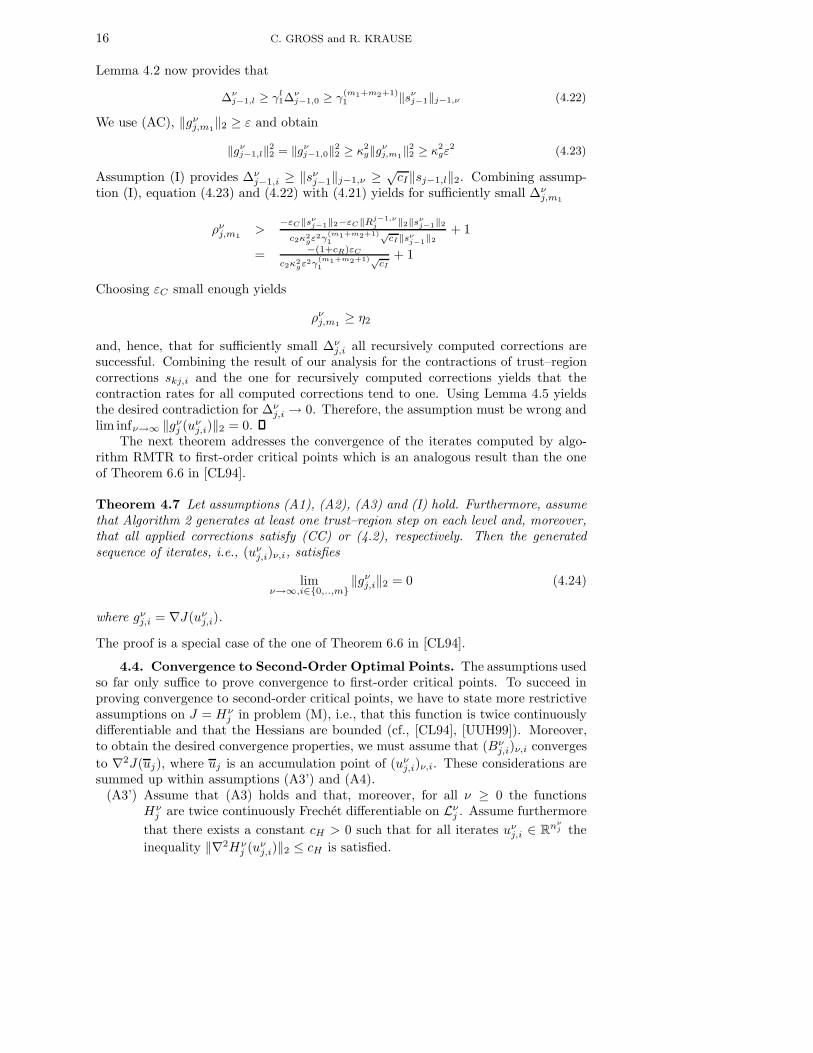
4.4. Convergence to Second-Order Optimal Points. The assumptions usedso far only suffice to prove convergence to first-order critical points. To succeed inproving convergence to second-order critical points, we have to state more restrictiveassumptions on J = Hν

j in problem (M), i.e., that this function is twice continuouslydifferentiable and that the Hessians are bounded (cf., [CL94], [UUH99]). Moreover,to obtain the desired convergence properties, we must assume that (Bν

j,i)ν,i converges

to ∇2J(uj), where uj is an accumulation point of (uνj,i)ν,i. These considerations are

summed up within assumptions (A3’) and (A4).(A3’) Assume that (A3) holds and that, moreover, for all ν ≥ 0 the functions

Hνj are twice continuously Frechet differentiable on Lν

j . Assume furthermore

that there exists a constant cH > 0 such that for all iterates uνj,i ∈ Rnν

j the

inequality ‖∇2Hνj (uν

j,i)‖2 ≤ cH is satisfied.


(A4) For all accumulation points uj of the sequence (uνj,i)ν,i and all ε > 0 we

assume that there exists an δ > 0 such that

‖uνj,i − uj‖2 ≤ δ ⇒ ‖Bν

j,i −∇2Jj(uj)‖2 ≤ ε (4.25)

(A5) For all accumulation points uj of the sequence (uνj,i)ν,i we assume that there

exists an ν0 ∈ N such that for all ν ≥ ν0 and all k > kν the following holds

λmin(∇2Jj(uj)) < 0 ⇒ ∃λH > 0 : λmin(∇2Hνk (P k,ν

k+1 · · ·Pj−1,νj uj)) < −λH

Additionally we assume that for all ε > 0 there exists an δ > 0 such that

‖uνj,i − uj‖2 ≤ δ and uν

k,i = uνk,0 = P

k,νk+1 · · ·P

j−1,νj uν

j,m1

⇒ ‖Bνk,i −∇2Hν

k (P k,νk+1 · · ·P

j−1,νj uj)‖2 ≤ ε

(4.26)

Now, a more restrictive acceptance criterion for the trust–region corrections is given.Let constants β1 ≥ βs, β

νk ≥ β0 > 0 for all k, ν exist, such that for all trust–region

corrections sk,i in Algorithm 1 it holds:

φνk,i(sk,i) < βν

kφν,0k,i s.t. ‖sk,i‖k,ν ≤ ∆ν

k,i (CC2)

where

φν,0k,i = min

s∈s∈Rnν

k |‖s‖k,ν≤∆νk,i

φνk,i(s) (4.27)

For the remainder of this section it is assumed that this condition replaces the firstCauchy decrease condition presented in Section 3. Note that (CC2) is more restrictivethan (CC) and, hence, Theorem 4.7 stays valid.Similar to Lemma 7.2 in [UUH99], the following Lemma provides a new decreaseestimation replacing the one given in Lemma 4.3.

Lemma 4.8 Let assumptions (A1), (A2), (A3’), (A4) and (I) hold and let the trust–region correction sk,i ∈ Rnν

k satisfy the Cauchy condition (CC2). If for uνk,i there

exists a variable λ > 0 and hνk,i ∈ Rnν

k with ‖hνk,i‖2 = 1 such that

〈hνk,i, B

νk,ih

νk,i〉 ≤ −λ‖hν

k,i‖22

then

predνk,i(sk,i) ≥

β0λ

2(∆ν

k,i)2 (4.28)

Proof. We assume that these assumptions hold and define

snk,i = ±∆ν

k,ihνk,i

Obviously, snk,i satisfies ‖sn

k,i‖2 ≤ ∆νk,i and it holds φν

k,i(snk,i) ≥ φ

ν,0k,i (cf. equation

(4.27)). We assume that the sign of snk,i is such that 〈gν

k,i, snk,i〉 ≤ 0. Using (CC2)

yields

φνk,i(sk,i) ≤ βν

kφνk,i(s

nk,i) = βν

k 〈gνk,i, s

nk,i〉 +

βνk

2 〈snk,i, B

νk,is

nk,i〉

≤ βνk

2 〈snk,i, B

νk,is

nk,i〉 ≤ −βν

k λ2 ‖sn

k,i‖22 = −βν

k λ2 (∆ν

k,i)2

Using the identity predνk,i(sk,i) = −φν

k,i(sk,i) completes the proof. Now the finalresult of this section is presented: The sequence of iterates created by Algorithm2 converges to second-order optimal points. This theorem extends the results ofTheorem 7.3 in [UUH99], to the context of the RMTR algorithm.


Theorem 4.9 Let assumptions (A1), (A2), (A3’), (A4), (A5) and (I) hold and thesequence (uν

j,i)ν,i be generated by algorithm RMTR using at least one trust–region step

on each level. Assume that all trust–region corrections sk,i ∈ Rnνk satisfy (CC2) and

that all sk,m1 , computed recursively, satisfy (4.2). Then, every accumulation pointu ∈ Rnj of (uν

j,i)ν,i satisfies the second-order necessary conditions, i.e.,

‖gj(u)‖2 = 0 (4.29)

〈s,∇2Jj(u)s〉 ≥ 0 ∀s ∈ Rn (4.30)

Proof. In Theorem 4.7 we have already shown that under the assumptions ofthe present theorem at every accumulation point of (uν

j,i) equation (4.29) is satisfied.Now, we prove that equation (4.30) holds by contradiction. Assume that (4.30) doesnot hold. Then there exists an c > 0 and an s ∈ Rnν

k such that

〈s,∇2Jj(u)s〉 < −c < 0 ∀ν ≥ ν0 ∈ N and k ∈ j, j − 1 (4.31)

Now, we choose ε > 0 and, hence, by (A4) there exists an δ > 0 such that it holds

〈s,∇2Jj(u)s〉 = 〈s,Bνj,is〉 + 〈s, (∇2Jj(u) −Bν

j,i)s〉≥ 〈s,Bν

j,is〉 − ε‖s‖22

(4.32)

Hence, we can choose ε small enough such that there exists an s with ‖s‖2 = 1 and

0 > ε‖s‖22 − c ≥ 〈s, Bν

j,is〉

This yields

〈s, Bνj,is〉 < −c′

for all ‖uνj,i − u‖2 ≤ δ where c′ > 0. For the other levels kν ≤ k < j we obtain, using

the same argumentation and defining uνk = P

k,νk+1 · · ·P

j−1,νj u,

〈s,∇2Hνk (uν

k)s〉 = 〈s,Bνk,is〉 + 〈s, (∇2Hν

j−1(uνk) −Bν

k,i)s〉≥ 〈s,Bν

k,is〉 − ε‖s‖22

(4.33)

for all pairs (k, i) such that uνk,i = uν

k,0 = Pk,νk+1 · · ·P

j−1,νj uν

j,m1.

In turn, we can use Lemma 4.8 and obtain that

predνk,i(sk,i) ≥ c(∆ν

k,i)2 (4.34)

holds for all sk,i satisfying (CC2), if uνj,m1

satisfies ‖uνj,m1

− u‖2 ≤ δ. Hence, we get

predνk,i(sk,i) ≥ c(∆ν

k,i)2 ≥ cγ

(m1+m2+1)·j1 (∆ν

j,m1)2 = c(∆ν

j,m1)2 (4.35)

Now, we choose ∆ > 0 and show that (4.34) implies that in a neighborhood of u eachcorrection reduces the energy of Jj by a constant factor, i.e., c(∆, δ) > 0, and, hence,u can not be an accumulation point.

1) If ∆νj,i ≥ ∆, we obtain for all successful trust–region corrections

J(uνj,i) − J(uν

j,i+1) ≥ η1predνj,i(sj,i) ≥ η1c∆

2 (4.36)


Now, let sk,i denote the first successful propagated trust–region correction. Hence,for successful recursions we obtain by reformulating ρν

k,m1≥ η2:

Hνk (uν

k,m1) −Hν

k (uνk,m1

+ sk,m1) ≥ η2(Hνk−1(u

νk−1,mν

k−1) −Hν

k−1(uνk−1,0))

≥ η22predν

k,i(sk,i) ≥ (η2)2c(∆ν

k−1,m1)2

= c(∆νk−1,m1

)2 ≥ c∆2

Now, we employ the argumentation in Lemma 4.4, equation (4.12) and obtain

J(uνj,m1

) − J(uνj,m1+1) ≥ cη1∆

2 (4.37)

where c > 0, independend from ν, k, i.2) Assume that ∆ν

j,i < ∆. Then, we employ ‖sj,i‖2 ≤ ∆νj,i, (A3’) and (A4), as well

as (4.12), Taylor’s Theorem and in combination with a possible reduction of ε, and∆ and obtain

predνj,i(s

νj,i)|ρν

j,i − 1| = |Jj(uνj,i + sj,i) − Jj(u

νj,i) − φν

j,i(sj,i)|= 1

2 |〈sj,i, (∇2Jj(uνj,i + τν

j,isj,i) −Bνj,i)sj,i〉|

≤ 12‖sj,i‖2

2 ‖∇2Jj(uνj,i + τν

j,isj,i) −∇2Jj(u)‖2

+ 12‖sj,i‖2

2 ‖∇2Jj(u) −Bνj,i‖2

≤ (1 − η2)c(∆νj,i)

2 ≤ (1 − η2)predνj,i(sj,i)

where τνj,i ∈ (0, 1). This yields

predνj,i(s

νj,i)|ρν

j,i − 1| ≤ (1 − η2)predνj,i(sj,i) (4.38)

Hence, for all pairs (ν, i) with ‖sj,i‖2 ≤ ∆ and ‖uνj,i − u‖2 ≤ δ it holds that ρν

j,i ≥ η2.We emphasize that the same argumentation holds for sufficiently small ∆ and thefirst successful and propagated trust–region correction. Assume that sk,i is such atrust–region correction. Then we obtain

Hνk (uν

k,mνk) −Hν

k (uνk,0) ≥ Hν

k (uνk,i+1) −Hν

k (uνk,i)

≥ η1predνk,i(sk,i)

≥ η1c(∆νk,m1

)2

Now, we employ the previous equation, and the argumentation and notation in The-orem 4.6, in particular equation (4.20) and obtain for sufficiently small ∆ and εC

ρνk+1,m1

≥ −εC‖sνk‖2−εc‖Rk,ν

k+1‖‖sνk‖2

Hνk (uν

k,0)−Hνk (uν

k,0−sνk) + 1

≥ −−εC‖sνk‖2−εc‖Rk,ν

k+1‖‖sνk‖2

c∆νk,i

+ 1


k+1‖‖sνk‖2

c∆νk+1,m1

+ 1


k+1‖‖sνk‖2

c‖sνk‖2

+ 1

≥ 1 − cεC

Hence, we can choose ∆ and εC sufficiently small such that sk+1,m1 is successful.Now, we use the implication

ρνk+1,m1

≥ η2⇒ Hν

k+1(uνk+1,m1

) −Hνk+1(u

νk+1,m1

+ sk+1,m1) ≥ η2(Hνk+1(u

νk,0) −Hν

k (uνk,mν

k))


In combination with (4.35) this yields

Hνk+1(u

νk+1,m1

) −Hνk+1(u

νk+1,m1

+ sk+1,m1) ≥ c∆νj,m1

Now, we deduce inductively that Jj(uνj,m1

) − Jj(uνj,m1

+ sj,m1) ≥ c∆νj,m1

. Carryingout this argumentation, we obtain that for sufficiently small ∆ and εC there will besuccessful coarse level corrections, i.e., ρν

j,m1≥ η2.

Finally, we obtain that such sj,i – computed either as trust–region step or recur-sively – will be applied if ∆ is chosen sufficiently small and, hence, ∆ν

j,i+1 ≥ ∆νj,i.

This yields that we can use the argumentation of the proof of Theorem 7.3 in [UUH99]and obtain for the case ∆j,i < ∆ that there is an infinite number of corrections induc-ing an actual reduction bounded from below by a constant factor. This factor onlydepends on ∆ or δ. In turn, this yields limν→∞,i Jj(u

νj,i) = −∞ which contradicts

the boundedness of Jj on L0j . This proves the proposition.

4.5. Convergence Speed. One important property of trust–region algorithmsis that under certain assumptions the computed iterates converge quadratically tolocal solutions (cf., [CL94]). We will now conclude our analysis of the RMTR algo-rithm and show that the iterates computed using Algorithm 1 converge under certainassumptions locally quadratic to a solution of problem (M).Now we introduce the notation: For a given iterate uν

j,i and radius ∆νj,i the unre-

stricted Newton step sν,Nj,i ∈ Rnν

j is defined as

sν,Nj,i = (Bν

j,i)−1gν

j,i (4.39)

if (Bνj,i)

−1 exists. Moreover, we define τν,∗j,i ∈ R as the solution of

φνj,i(τ

ν,∗j,i s

ν,Nj,i ) = minφν

j,i(τsν,Nj,i ) | τ ≥ 0 such that ‖τsν,N

j,i ‖2 ≤ ∆νj,i

Now we can prove the following theorem (cf., [CL94]).

Theorem 4.10 Assume that the assumptions of Theorem 4.9, (A3’) hold and, inparticular, that Bν

j,i is always chosen as ∇2Jj(uνj,i), as well as, that the constant βν

j

in (CC2) satisfies βνj > 1. Moreover, assume that (uν

j,i)ν,i tends to one limit point u

with non-singular Hessian. Now, let sν,Nj,i be the Newton step as defined by (4.39), if

it exists, and let sj,i = τν,∗j,i s

ν,Nj,i whenever τν,∗

j,i sν,Nj,i satisfies (CC2).

Then for sufficiently large ν the iterates (uνj,i)ν,i computed employing Algorithm 1

converge quadratically to u.

Proof. First, note that (A2) and (A3) imply that ∇Jj is locally Lipschitz contin-

uous and, hence, if the sequence of unrestricted Newton steps (sν,Nj,i )ν,i exists and is

applied to generate a sequence of iterates uνj,i, this sequence would converge quadrat-

ically to u.Now, it will be shown that sj,i = τ

ν,∗j,i s

ν,Nj,i for all sufficiently large ν. Note that due to

Theorem 4.9 and due to the assumption that ∇2Jj(uνj,i) is invertible we obtain that

∇2Jj(uνj,i) is positive definite. Hence, Theorem 4.9 provides that ∆ν

j,i is bounded from

below and gνj,i tends to zero and, therewith, we obtain that ‖sν,N

j,i ‖2 and ‖τν,∗j,i s

ν,Nj,i ‖2

tend to zero as well. Now, for sufficiently large ν, ψνj,i becomes a convex function,


sν,Nj,i is a global minimizer of ψν

j,i and, hence, satisfies (CC2) for sufficient large ν. In

turn, we obtain for sufficiently small ‖sν,Nj,i ‖2 and ‖uν

j,i − u‖2

‖sν,Nj,i ‖2 ≤ ‖uν

j,i−u‖2+‖uνj,i−1−u‖2 = O(‖uν

j,i−u‖2)+O(‖uνj,i−u‖2

2) = O(‖uνj,i−u‖2)

due to the local convergence properties of Newton corrections (cf., [Deu04]). Thisyields for ν sufficiently large that |τν,∗

j,i − 1| = O(‖uνj,i − u‖2) and, hence,

‖τν,∗j,i s

ν,Nj,i − s

ν,Nj,i ‖2 ≤ |τν,∗

j,i − 1|‖sν,Nj,i ‖2

= O(‖uνj,i − u‖2

2)

Since for sufficiently large ν we have ‖uνj,i+s

ν,Nj,i −u‖2 = O(‖uν

j,i−u‖22) and, therefore,

‖uνj,i+1 − u‖2 ≤ ‖uν

j,i + sν,Nj,i − u‖2 + ‖sν,N

j,i − τν,∗j,i s

ν,Nj,i ‖2

= O(‖uνj,i − u‖2

2)

for ‖uνj,i − u‖2 ≤ 1.

Note, that there is the possibility that the previous iterate has been updated usingthe recursion. Then one obtains by Theorem 4.7 that ‖uν

j,i − u‖2 ≤ ‖uνj,i−1 − u‖2

which yields the following relation between the surrounding trust–region steps uνj,i+1

and uνj,i−1: ‖uν

j,i+1 − u‖2 = O(‖uνj,i − u‖2

2) = O(‖uνj,i−1 − u‖2

2).This completes the proof.

5. Numerical Examples. In this section, we present results illustrating thebehavior of our RMTR algorithm for boundary value problems from the field of linearand non-linear elasticity. Our RMTR algorithm, as presented in this work, was imple-mented in ObsLib++ [Kra07], UG [BBJ+97], respectively. Moreover, the examplespresented in this section, depend on the import of meshes given in Exodus II format[SY94] and parameters stored in Exodus parameter files [Gro08].

5.1. Linear Elasticity. Here, we consider the solution of the following boundaryvalue problem

∫

Ω

1

2σ(u) : ε(u) − f · u dx+

∫

Ω

g · u dx

where ε(u) = 12 (∇uT + ∇u) denotes the linearized Green – St. Venant strain tensor

and

σ(ε) =E

1 + νε(u) +

ν

1 − 2νtr (ε(u)) I

Hooke’s tensor [Cia88, Bra07]. In our numerical experiment we chose f ≡ 0, E = 300,ν = 0.1, as well as Ω = (x, y, z)| − 0.5 ≤ x, y, z ≤ 0.5. The boundary values areDirichlet values g causing a rotation by 45 about the x axis of (x, y, z)| − 0.5 ≤z, y ≤ 0.5, x = 0.5, as well as zero Dirichlet values for all (x, y, z)| − 0.5 ≤ z, y ≤0.5, x = −0.5. All other boundary values are set to homogeneous Neumann values, asillustrated in the left image of Figure 5.1. Here, the deformed mesh and the resultingvon Mises stresses are shown.The right picture of Figure 5.1 shows a comparison of the reduction of the first-ordersufficiency conditions induced by a “single–level” trust–region strategy and the RMTRstrategy. Here, a single–level strategy means the computation only on the finest level.


Hence, the dashed line in the right image of Figure 5.1 represents the norm of thegradient after m1 +m2 smoothing steps, the solid line represents the gradient’s normat the end of each V-cycle.Here, we used two pre– and two post–smoothing trust-region steps (on each level).However, in our computations we use the equivalence of ‖·‖2 and ‖·‖∞ and transformthe trust–region constraint ‖s‖2 ≤ ∆ into ‖s‖∞ ≤ ∆. This makes the application ofa projected cg–algorithm possible. Hence, the quadratic minimization problems weresolved approximately by 50 projected cg–steps on the coarsest level and 10 projectedcg–steps on the finer levels, respectively. The initial solution in both simulations wasu ≡ 0 on Ω.

Fig. 5.1. Elliptic boundary value problem (135, 456 degrees of freedom). Left image: De-formed mesh, boundary values, von Mises stress distribution. Right diagram: Comparison of first-order sufficiency condition, i.e., ‖gν

j,0‖2, between RMTR and a “single–level” trust–region strategy

5.2. Non-Linear Elasticity. R. W. Ogden introduced in [Ogd97] a material lawfor rubber-like materials. The associated stored energy function is highly non-lineardue to a penalty term which prevents the inversion of element volumes:

W (∇ϕ) = a · trE + b · (trE)2 + c · tr(E2) + d · Γ(det(∇ϕ)) (5.1)

where ϕ = id + u. This function is a polyconvex stored energy function depending onthe the Green – St. Venant strain tensor E(u), i.e., E(u) = 1

2 (∇uT +∇u+∇uT∇u),a penalty function Γ(x) = − ln(x) for x ∈ R+, and

a = −dΓ′(1), b = 12 (λ− d(Γ′(1) + Γ′′(1))),

c = µ+ dΓ′(1), d > 0

In our computations we used the parameters λ = 34, µ = 136, d = 100.

1. We consider the same geometry and boundary values as for the previousexample. The solution of the minimization problem induced by the non-linear stored energy function (5.1) yields the results in Figure 5.2 and Figure5.3. The first image in Figure 5.3 shows the deformed mesh, Dirichlet values,as well as the von Mises stresses.The left diagram of Figure 5.2 shows a comparison of the RMTR algorithmand a “single–level” trust–region strategy: The solid line represents the normof the gradient at the end of each V-cycle, the dashed line shows the gradient’snorm after m1 + m2 trust–region corrections on the finest level. For this


1e-10

1e-08

1e-06

1e-04

0.01

1

100

0 5 10 15 20 25

Nor

m o

f the

Gra

dien

t

Performed V-Cycles

First-Order Sufficiency Condition

RMTRSinglelevel Trust--Region Strategy

Fig. 5.2. Non-linear boundary value problem, Problem 1 with 107, 811 degrees of freedom.Left diagram: Comparison of RMTR algorithm and a “single–level” trust–region strategy: First-order sufficiency conditions, i.e., ‖gν

j,0‖2 at the end of each RMTR V-cycle and after each m1 +m2 fine–level trust–region smoothing steps, respectively. Right diagram: First order sufficiencyconditions for the “Single–level“ strategy with m1 = 0 and m2 = 1 trust–region smoothing steps andexact solution of the occurring constrained quadratic minimization problems (i.e., (3.2)

Fig. 5.3. Non-linear boundary value problems. Deformed meshes, Dirichlet values and vonMises stress distributions. Left image: Solution of Problem 1 with 135, 456 degrees of freedom. Rightimage: Solution of Problem 2 with 1, 032, 768.

computation we set m1 = m2 = 2, computed 50 projected cg iterations onthe coarsest level, and 10 projected cg iterations on the other levels to solve(3.1).The right diagram shows the gradient’s behavior while solving the quadraticminimization problems (3.1) exactly (cf., Section 4.5) using the “single–level”trust–region strategy with m1 = 0 and m2 = 1.

2. This simulation uses the domain Ω = (x, y, z)|(−0.5 ≤ x, y, z ≤ 0.5) ∧¬((−0.15 < x < 0.15) ∧ (−0.15 < y < 0.15)). Boundary values were givenby the following Dirichlet values

g((x, y, z)T ) =

(0.2, 0, 0)T if x = 0.5

0 otherwise

The solution of the non-linear boundary value problem induced by equation(5.1) on this geometry (meshed with 1, 032, 768 degrees of freedom) and thechosen boundary values induce the deformations and von Mises stresses shownin the right image in Figure 5.3. The reduction of the first–order sufficiency


1e-08

1e-07

1e-06

1e-05

1e-04

0.001

0.01

0.1

1

10

100

0 5 10 15 20 25

Nor

m o

f the

Gra

dien

t

Performed V-Cycles


RMTRCascadic Multigrid

RMTR - nested iterationSinglelevel - Trust-Region-Strategy

1e-08

1e-06

1e-04

0.01

1

100

10000

1e+06

0 5 10 15 20 25 30 35 40

Nor

m o

f the

Gra

dien

t

Performed V-Cycles


RMTRSinglelevel Trust--Region Strategy

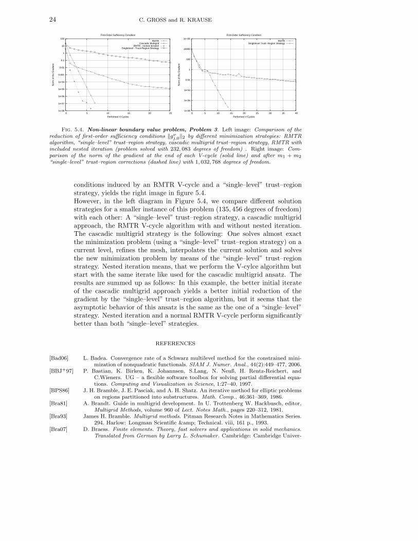
Fig. 5.4. Non-linear boundary value problem, Problem 3. Left image: Comparison of thereduction of first-order sufficiency conditions ‖gν

j,0‖2 by different minimization strategies: RMTRalgorithm, “single–level” trust–region strategy, cascadic multigrid trust–region strategy, RMTR withincluded nested iteration (problem solved with 232, 083 degrees of freedom) . Right image: Com-parison of the norm of the gradient at the end of each V-cycle (solid line) and after m1 + m2

“single–level” trust–region corrections (dashed line) with 1, 032, 768 degrees of freedom.

conditions induced by an RMTR V-cycle and a “single–level” trust–regionstrategy, yields the right image in figure 5.4.However, in the left diagram in Figure 5.4, we compare different solutionstrategies for a smaller instance of this problem (135, 456 degrees of freedom)with each other: A “single–level” trust–region strategy, a cascadic multigridapproach, the RMTR V-cycle algorithm with and without nested iteration.The cascadic multigrid strategy is the following: One solves almost exactthe minimization problem (using a “single–level” trust–region strategy) on acurrent level, refines the mesh, interpolates the current solution and solvesthe new minimization problem by means of the “single–level” trust–regionstrategy. Nested iteration means, that we perform the V-cylce algorithm butstart with the same iterate like used for the cascadic multigrid ansatz. Theresults are summed up as follows: In this example, the better initial iterateof the cascadic multigrid approach yields a better initial reduction of thegradient by the “single–level” trust–region algorithm, but it seems that theasymptotic behavior of this ansatz is the same as the one of a “single–level”strategy. Nested iteration and a normal RMTR V-cycle perform significantlybetter than both “single–level” strategies.

REFERENCES

[Bad06] L. Badea. Convergence rate of a Schwarz multilevel method for the constrained mini-mization of nonquadratic functionals. SIAM J. Numer. Anal., 44(2):449–477, 2006.

[BBJ+97] P. Bastian, K. Birken, K. Johannsen, S.Lang, N. Neuß, H. Rentz-Reichert, andC.Wieners. UG – a flexible software toolbox for solving partial differential equa-tions. Computing and Visualization in Science, 1:27–40, 1997.

[BPS86] J. H. Bramble, J. E. Pasciak, and A. H. Shatz. An iterative method for elliptic problemson regions partitioned into substructures. Math. Comp., 46:361–369, 1986.

[Bra81] A. Brandt. Guide in multigrid development. In U. Trottenberg W. Hackbusch, editor,Multigrid Methods, volume 960 of Lect. Notes Math., pages 220–312, 1981.

[Bra93] James H. Bramble. Multigrid methods. Pitman Research Notes in Mathematics Series.294. Harlow: Longman Scientific & Technical. viii, 161 p., 1993.

[Bra07] D. Braess. Finite elements. Theory, fast solvers and applications in solid mechanics.Translated from German by Larry L. Schumaker. Cambridge: Cambridge Univer-


sity Press. 17, 2007.[CGT00] A. R. Conn, N. I. M. Gould, and Ph. L. Toint. Trust-region methods. Society for

Industrial and Applied Mathematics, Philadelphia, PA, USA, 2000.[Cia88] P. G. Ciarlet. Mathematical elasticity, volume I: Three-dimensional elasticity. Studies

in Mathematics and its Applications, 20(186):715–716, 1988.[CL94] T. F. Coleman and Y. Li. On the convergence of interior-reflective Newton methods for

nonlinear minimization subject to bounds. Math Programming, 67:189–224, 1994.[Dah97] Wolfgang Dahmen. Wavelet and multiscale methods for operator equations. Iserles,

A. (ed.), Acta Numerica Vol. 6, 1997. Cambridge: Cambridge University Press.55-228 (1997)., 1997.

[Deu04] P. Deuflhard. Newton methods for nonlinear problems – affine invariance and adaptivealgorithms. Springer Series in Computational Mathematics 35. Berlin: Springer.xii, 2nd edition, 2004.

[GO95] M. Griebel and P. Oswald. On the abstract theory of additive and multiplicativeSchwarz algorithms. Numer. Math, 70:163–180, 1995.

[Gro08] C. Groß. Import of geometries and extended informations into obslib++ using theexodus ii and exodus parameter file formats. Technical Report 712, Institute forNumerical Simulation, University of Bonn, Germany, January 2008.

[GST06] S. Gratton, A. Sartenaer, and P. L. Toint. Recursive trust-region methods for multiscalenonlinear optimization. Technical report, Cerfacs, 2006.

[KKS+06] R. Kornhuber, R. Krause, O. Sander, P. Deuflhard, and S. Ertel. A monotone multigridsolver for two body contact problems in biomechanics. Springer, Computing andVisualization in Science, 2006.

[Kor97] R. Kornhuber. Adaptive monotone multigrid methods for nonlinear variational prob-lems. B.G. Teubner, Stuttgart, 1997.

[Kra07] R. Krause. A parallel decomposition approach to non-smooth minimization problems- concepts and implementation. Technical Report 709, Institute for NumericalSimulation, University of Bonn, Germany, 2007.

[Lev44] K. Levenberg. A method for the solution of certain non-linear problems in least squares.Q. Appl. Math., 2:164–168, 1944.

[LHKK79] C. L. Lawson, R. J. Hanson, D. Kincaid, and F. T. Krogh. Basic linear algebra sub-programs for Fortran usage. ACM Trans. Math. Soft., 5:308–323., 1979.

[LN05] Robert Michael Lewis and Stephen G. Nash. Model problems for the multigrid op-timization of systems governed by differential equations. SIAM J. Sci. Comput.,26(6):1811–1837, 2005.

[Mar63] D.W. Marquardt. An algorithm for least-squares estimation of nonlinear parameters.J. Soc. Ind. Appl. Math., 11:431–441, 1963.

[Mor78] J.J. More. The Levenberg-Marquardt algorithm: implementation and theory. Lect.Notes Math., 630:105–116, 1978.

[Nas00] S. G. Nash. A multigrid approach to discretized optimization problems. Journal ofOptimization Methods and Software, 14:99–116, 2000.

[Ogd97] R. W. Ogden. Non-linear elastic deformation. Dover Publications; New Edition, 1997.[Osw94] P. Oswald. Multilevel finite element approximation. Theory and applications. Teubner

Skripten zur Numerik. Stuttgart: B. G. Teubner., 1994.[SG04] O. Schenk and K. Gartner. Solving unsymmetric sparse systems of linear equations

with pardiso. Journal of Future Generation Computer Systems, 20(3):475–487,2004.

[SY94] L. Schoof and V. Yarberry. Exodus II: A finite element data model. Technical report,Schoof, L. A., Yarberry, V. R., EXODUS II: A Finite Element Data Model, SandiaNational Laboratories Technical Report, SAND92–2137, Albuquerque, NM (1994).,1994.

[TE98] X.-C. Tai and M. S. Espedal. Rate of convergence of some space decomposition methodsfor linear and non-linear elliptic problems. SIAM J. Numer. Anal., 35:1558–1570,1998.

[UUH99] M. Ulbrich, S. Ulbrich, and M. Heinkenschloss. Global convergence of trust-regioninterior-point algorithms for infinite-dimensional nonconvex minimization subjectto pointwise bounds. SIAM Journal on Control and Optimization, 37(3):731–764,1999.

[WB06] A. Waechter and L. T. Biegler. On the implementation of an interior-point filter line-search algorithm for large-scale nonlinear programming. Mathematical Program-ming, 106(1):25–57, 2006.

Bestellungen nimmt entgegen: Institut für Angewandte Mathematik der Universität Bonn Sonderforschungsbereich 611 Wegelerstr. 6 D - 53115 Bonn Telefon: 0228/73 4882 Telefax: 0228/73 7864 E-mail: [email protected] http://www.sfb611.iam.uni-bonn.de/

Verzeichnis der erschienenen Preprints ab No. 370

370. Han, Jingfeng; Berkels, Benjamin; Droske, Marc; Hornegger, Joachim; Rumpf, Martin; Schaller, Carlo; Scorzin, Jasmin; Urbach Horst: Mumford–Shah Model for One-to-one Edge Matching; erscheint in: IEEE Transactions on Image Processing 371. Conti, Sergio; Held, Harald; Pach, Martin; Rumpf, Martin; Schultz, Rüdiger: Shape Optimization under Uncertainty – a Stochastic Programming Perspective 372. Liehr, Florian; Preusser, Tobias; Rumpf, Martin; Sauter, Stefan; Schwen, Lars Ole: Composite Finite Elements for 3D Image Based Computing 373. Bonciocat, Anca-Iuliana; Sturm, Karl-Theodor: Mass Transportation and Rough Curvature Bounds for Discrete Spaces 374. Steiner, Jutta: Compactness for the Asymmetric Bloch Wall 375. Bensoussan, Alain; Frehse, Jens: On Diagonal Elliptic and Parabolic Systems with Super-Quadratic Hamiltonians 376. Frehse, Jens; Specovius-Neugebauer, Maria: Morrey Estimates and Hölder Continuity for Solutions to Parabolic Equations with Entropy Inequalities 377. Albeverio, Sergio; Ayupov, Shavkat A.; Omirov, Bakhrom A.; Turdibaev, Rustam M.: Cartan Subalgebras of Leibniz n-Algebras 378. Schweitzer, Marc Alexander: A Particle-Partition of Unity Method – Part VIII: Hierarchical Enrichment 379. Schweitzer, Marc Alexander: An Algebraic Treatment of Essential Boundary Conditions in the Particle–Partition of Unity Method 380. Schweitzer, Marc Alexander: Stable Enrichment and Local Preconditioning in the Particle– Partition of Unity Method 381. Albeverio, Sergio; Ayupov, Shavkat A.; Abdullaev, Rustam Z.: Arens Spaces Associated with von Neumann Algebras and Normal States 382. Ohta, Shin-ichi: Finsler Interpolation Inequalities 383. Fang, Shizan; Shao, Jinghai; Sturm, Karl-Theodor: Wasserstein Space Over the Wiener Space

384. Nepomnyaschikh, Sergey V.; Scherer, Karl: Multilevel Preconditioners for Bilinear Finite Element Approximations of Diffusion Problems 385. Albeverio, Sergio; Hryniv, Rostyslav; Mykytyuk, Yaroslav: Factorisation of Non-Negative Fredholm Operators and Inverse Spectral Problems for Bessel Operators 386. Otto, Felix: Optimal Bounds on the Kuramoto-Sivashinsky Equation 387. Gottschalk, Hanno; Thaler, Horst: A Comment on the Infra-Red Problem in the AdS/CFT Correspondence 388. Dickopf, Thomas; Krause, Rolf: Efficient Simulation of Multi-Body Contact Problems on Complex Geometries: A Flexible Decomposition Approach Using Constrained Minimization 389. Groß, Christian; Krause, Rolf: On the Convergence of Recursive Trust-Region Methods for Multiscale Non-Linear Optimization and Applications to Non-Linear Mechanics

On the Convergence of Recursive Trust-Region Methods for...

Documents

Transcript of On the Convergence of Recursive Trust-Region Methods for...