On the bass note of a Schottky group

Peter G. Doyle

Version 1.01A129 August 1994

Abstract

Using a classical method from physics called Rayleigh’s cutting

method, we prove the conjecture of Phillips and Sarnak that there is a

universal lower bound L2 > 0 for the lowest eigenvalue of the quotient

manifold of a classical Schottky group Γ acting on hyperbolic 3-space

H3. By work of Patterson and Sullivan, this implies that there is a

universal upper bound U2 < 2 for the Hausdorff dimension of the limit

set of Γ, or equivalently, for the critical exponent of the Poincare series

associated with Γ. The latter implication answers a question that can

be traced back to Schottky and Burnside.

1 Introduction

1.1 Classical Schottky groups

Let C1, . . . , Cn be a collection of circles in the Riemann sphere that bounddisjoint open disks D1, . . . , Dn. Note that circles may be tangent, but other-wise they don’t intersect. (See Figure 1.) Let F denote the complement ofD1∪ . . .∪Dn, that is, the closure of the common exterior of C1, . . . , Cn. Sup-pose that n is even, and that for i = 1, . . . , n/2 we have specified a Mobiustransformation γi mapping the exterior of C2i− 1 to the interior of C2i. Thegroup Γ of Mobius transformations generated by the gammai’s is a Kleiniangroup with fundamental domain F . It is called a classical Schottky group.

1

Figure 1: Circles in the Riemann sphere.

2

1.2 A lower bound for the bass note

View the Riemann sphere as the boundary of hyperbolic 3-space H3, andview Γ as a group of isometries of H3. Consider λ0(H

3/Γ), the bottom ofthe spectrum of the Laplacian ∆ = −div grad on H3/Γ (note the minussign). Except in trivial cases, λ0(H

3/Γ) is a bona fide eigenvalue; we call itthe “lowest eigenvalue” of H3/Γ, or of Γ. Physically, it is the square of thefrequency of the the bass note of H3/Γ—the lowest note you would hear ifyou hit H3/Γ with a mallet.

We will prove the conjecture of Phillips and Sarnak [13] that for anyclassical Schottky group Γ,

λ0(H3/Γ) ≥ L2 > 0,

where L2 is some universal constant.

1.3 Implications

Let δ(Γ) denote the exponent of convergence of the Poincare series

∑

γ

exp(−s(z, γw)),

where z, w are fixed points of H3 and (a, b) is the hyperbolic distance from ato b. Let d(Λ(Γ)) denote the Hausdorff dimension of the limit set Λ(Γ). Bywork of Patterson [11], [12] and Sullivan [17], [18],

δ(Γ) = d(Λ(Γ)),

andλ0(H

3/Γ) = δ(Γ)(2− δ(Γ)),

as long as δ(Γ) > 1. Thus our universal lower bound for λ0 implies a universalupper bound U2 < 2 for δ(Γ) and d(Λ(Γ)).

1.4 Some history

The problem of finding an upper bound for δ(Λ) can be traced back to Schot-tky [16]. Burnside [5] conjectured δ ≤ 1; this was disproved by Myrberg [9],[10]. Akaza [1], [2] gave examples with δ = 1.5. Sarnak [15] and Phillips

3

Figure 2: The Apollonian packing.

proved the existence of examples with δ ≥ 1.75. Phillips and Sarnak [13]conjectured the existence of a universal upper bound U2 < 2, and proved theanalogous result in higher dimensions. Brooks [4], [3] proved the conjecturefor the special class of groups for which the disks D1, . . . , Dn are a subsetof the disks of the Apollonian packing. (See Figure 2.) Phillips, Sarnak,and Brooks have suggested that the supremum of δ(Γ) over all such “Apollo-nian” Schottky groups should equal the supremum over all classical Schottkygroups, but this is not known.

1.5 Rayleigh’s cutting method

To get a lower bound for the bass note of H3/Γ, we will apply a classicalmethod from physics called Rayleigh’s cutting method. This method was in-troduced by Rayleigh [14] as a way of estimating the bass note of a Helmholtzresonator. The idea is to cut the system into pieces whose lowest eigenvaluecan be estimated, and then observe that if the lowest eigenvalue of each ofthe pieces is ≥ c, then the lowest eigenvalue of the original system is ≥ c.

1.6 Infinitely skinny tubes that grow more or less ex-

ponentially

In applying Rayleigh’s method, our approach will be to cut our manifoldinto an infinite number of infinitely skinny tubes. A crude estimate showsthat we can get a lower bound for the lowest eigenvalue of a tube as longas its cross-section grows more or less exponentially. Thus to get a lower

4

bound for the lowest eigenvalue of a manifold it suffices to show that it canbe cut into infinitely skinny tubes in such a way that the cross-section ofeach and (almost) every tube grows more or less exponentially. This resultcomplements the known fact that the rate of exponential growth of a manifoldgives an upper bound for the bass note. Here we have a sort of converse:A definite rate of exponential growth gives a lower bound for the bass note,provided that the growth can be “correlated” by means of tubes.

1.7 Plan

In section 2, we will make precise the notion of cutting a manifold into tubes,and show how a cutting into tubes gives a lower bound for the bass note. Asthe subject is physics and not geometry, the tone will be formal. In section3, we will show how to cut H3/Γ into tubes, so as to prove the existence of auniversal lower bound for λ0(H

3/Γ). Here we are back on solid ground, andthe tone will be more relaxed.

2 Cutting a manifold into tubes

2.1 The lowest eigenvalue λ0

Our goal is a method for getting lower bounds for the lowest eigenvalue λ0

of a manifold M . Among several equivalent definitions for λ0, the followingwill be most convenient to work with:

Definition. Let M be a non-compact complete n-dimensional Rieman-nian manifold with boundary. Let TF (M) (“test functions”) denote the setof C∞ functions u : M → [0,∞) that have compact support and do not van-ish identically. We define λ0(M) as the infimum over TF (M) of the Rayleighquotient

∫

M |gradu|2∫

M u2.

2.2 The cutting method

To estimate λ0, we will use Rayleigh’s cutting method (see Rayleigh [14],Maxwell [8]). This method belongs to a class of related methods knowncollectively as Rayleigh’s short-cut method. For a general discussion of

5

the short-cut method see Doyle and Snell [6]. (In the references given here,Rayleigh’s method is applied to conductance problems; the generalizationfrom conductance problems to bass-note problems is straight-forward.)

The cutting method is based on Rayleigh’s cutting law, one form of whichis the following:

Proposition. If M is obtained by gluing together parts of the boundaryof another manifold Mcut, then

λ0(M) ≥ λ0(Mcut).

Proof. This follows from the definition of λ0 that we have adopted. qed

2.3 Cutting into tubes

Our method for getting lower bounds for λ0 is based on cutting M up intoinfinitely skinny tubes. In other applications it will be most convenient toconsider tubes modeled on [0,∞) that begin inside the manifold and run outto infinity in one direction. Here, we will consider only tubes modeled on R

that run out to infinity in both directions. There are two excuses for this. Thefirst is that these doubly-infinite tubes are best for the specific applicationwe have in mind. The second is that you can always get a singly-infinite tubeby folding a doubly-infinite tube in half.

Definition. A cutting of M into tubes consists of a measure space T (toindex the tubes) and measurable maps

f : T ×R→M,

σ : T ×R→ [0,∞)

(to show how they run, and tell their cross-section) such that

• (i) f pushes the measure σ(τ, x)dτdx on T × tube over onto the Rie-mannian volume measure on M , that is, for any integrable function uon M , we have

∫

Mu =

∫

dτ∫

u(f(τ, x))σ(τ, x)dx.

(This makes precise the notion that σ tells the cross-section of thetube.)

6

• (ii) for almost all τ , the curve f(τ, ·) is piecewise C1, parametrized byarc length, and proper. (The tubes may zig-zag a little, but must runout to the boundary.)

• (iii) for almost all τ we have 0 <∫ ba σ(τ, x)dx < ∞ whenever −∞ <

a < b <∞. (The tubes are neither too fat nor too thin.)

2.4 Inhomogeneous strings

Our purpose in cutting M into tubes is to reduce our n-dimensional eigen-value problem to a bunch of 1-dimensional inhomogeneous string problems(Sturm-Liouville problems). An inhomogeneous string is described by twofunctions σ and ρ, telling its cross-section and its density as a function oflength. When we come to consider the strings that arise from our tubes, wewill want to set ρ = σ, to indicate that the mass per unit length is propor-tional to the cross-section. For the moment we will distinguish σ from ρ, notso much for the sake of generality as to make clearer their differing roles.

Definition. If σ : R → [0,∞) is measurable, and 0 <∫ ba σ(τ, x)dx < ∞

whenever −∞ < a < b < ∞, we will say that σ is neither too big nor too

small.

Thus (iii) above states that for almost all τ , σ(τ, ·) is neither too big nortoo small.

Definition. Letσ, ρ : R→ [0,∞)

be measurable, with σ and ρ neither too big nor too small. Then we defineλ0(σ, ρ) as the infimum over TF (R) of the Rayleigh quotient

∫

σ(

dφdx

)2dx

∫

ρφ2dx

2.5 Using piecewise differentiable test functions

Our method from converting information about the tubes into informationabout M will involve pulling back a test function on M to each of the tubes.The functions on the tubes that we will obtain in this way will not necessarilybe smooth, because we are allowing the tubes to zig-zag. It would be possibleto work only with cuttings into smooth tubes, but we prefer to allow ourselves

7

the extra latitude in cutting, and pay the price by smoothing the pulled-backtest functions, rather than the tubes themselves.

Lemma. If φ : R → [0,∞) is piecewise C1, has compact support, anddoesn’t vanish identically, then

∫

σ(

dφdx

)2dx

∫

ρφ2dx ≥ λ0(σ, ρ).

Proof. Choose b : R→ [0,∞) to be smooth, with support in the interval[−1, 1] and int1−1b(x)dx = 1, and convolve φ with 1

εb(x

ε). The result is a

member of TF (R) whose Rayleigh quotient approaches that of φ as ε → 0.qed

2.6 What the tubes tell us about the original space

We now show how to turn information about the lowest eigenvalues of thetubes into information about M . Note that in treating the tubes as inhomo-geneous strings, we set ρ = σ, as promised.

Proposition. Suppose M can be cut into tubes is such a way that foralmost all τ ,

λ0(σ(τ, ·), σ(τ, ·)) ≥ λ.

Then λ0(M) = λ.Proof. Let u be an element of TF (M). Then

∫

M|gradu|2 =

∫

dτ∫

σ(τ, x)|gradu(f(τ, x))|2dx

≥∫

dτ∫

σ(τ, x)

(

∂(u ◦ f)

∂x

)2

dx

(note the use of parametrization by arc length)

≥ λ∫

dτ∫

σ(τ, x)((u ◦ f)(τ, x))2dx

(note the need for properness of the tubes)

= λ∫

Mu2.♣

8

2.7 Twiddling σ and ρ

In estimating λ0 for our tubes, we will want to know what effect altering σand ρ by some bounded factor will have on λ0(σ, ρ). There are two reasonsfor this. The first is that when all we are after is a very conservative lowerbound for λ0, we may want to hack the space into tubes in such a way thatwe have only very gross information about the growth of the cross-sectionof the tubes. The second reason is that to get a lower bound for λ0(σ, ρ), itmay be convenient to assume that σ and ρ are pretty smooth.

Lemma. For any K (0 < K <∞),

λ0(Kσ, ρ) = λ0(σ, 1

Kρ) = Kλ0(σ, ρ).♣

Lemma. Let σ, ρ : R→ [0,∞) be measurable, with σ and ρ neither toobig nor too small. If

σ ≥ σ

andρ ≤ ρ,

thenλ0(σ, ρ) ≥ λ0(σ, ρ).♣

Lemma. Let σ, ρ : R→ [0,∞) be measurable, with σ and ρ neither toobig nor too small. Suppose that for constants K1, K2 (0 < K1, K2 <∞), wehave

σ ≥ 1

K1σ

andρ ≤ K2ρ.

Thenλ0(σ, ρ) ≥ 1

K1K2λ0(σ, ρ).♣

2.8 Estimating λ0 for a string

The great thing about a string is that it is easy to get lower bounds for thelowest eigenvalue by exhibiting an appropriate superharmonic function. Of

9

course the same thing works in higher dimensions, but it is easier to cook upa superharmonic function on the line than in n-space.

Rather than appeal to established theory, we will find it simplest to con-coct our own proof of how to get a lower bound for λ0 out of a suitablesuperharmonic function. This proof, which is based on some ideas of Hol-land [7], may seem a little mysterious. Its advantage is that it works directlywith the definition of λ0 that we have been using, rather than the definitionof λ0 as some kind of eigenvalue.

Lemma. If σ is piecewise C1, and if there is a C2 function φ0 : R →(0,∞) that satisfies

−; d

dx(

σdφ0

dx

)

≥ λρφ0

then λ0(σ, ρ) ≥ λ.Proof. Setting

φ0 = e−ψ0 ,

we find thatd

dx(

σdψ0

dx

)

− σ(

dψ0

dx

)2 ≥ λρ.

Let φ be in TF (R). Then

∫

σ

(

dφ

dx

)2

dx =∫

d

dx(

σdψ0

dx

)

φ2 + σ dψ0

dxddx

(φ2) + σ(

dφdx

)2

dx

(integration by parts)

=∫

d

dx(

σdψ0

dx

)

+ 2σ dψ0

dx

(

1

φdφ

dx

)

+ σ(

1

φdφ

dx

)2

φ2dx

=∫

d

dx(

σdψ0

dx

)

+ σ

dψ0

dx+

(

1

φdφ

dx

)

sup2− σ(

dψ0

dx

)2

φ2dx

10

(completing the square)

≥∫

d

dx(

σdψ0

dx

)

− σ(

dψ0

dx

)2

φ2dx

≥ λ∫

ρφ2dx.♣

2.9 Tubes that grow more or less exponentially

If the cross-section σ of a tube does not grow exponentially in one directionor the other, there is no hope that λ0(σ, σ) will be positive. The reason isthat λ0(σ, σ) measures the exponential rate of decay of the heat kernel forthe tube, and since the flow of heat along the tube is slow and no heat islost, the temperature can’t decay exponentially unless there is an exponentialamount of material over which to distribute the heat.

On the other hand, if σ is growing exponentially with a certain minimumrate, and if it doesn’t waver too much, then we can get a positive lowerbound for λ0(σ, σ). The bigger the minimum growth rate and the smallerthe amount of wavering, the better the lower bound will be.

Lemma. Suppose thatσ(x) = eA(x),

where A : R→ R is piecewise C1 and

dA

dx ≥ a > 0.

Thenλ0(σ, σ) ≥ a2

4.

Proof. Letφ0(x) = e−

a2x.

Then−d

dx(

σdφ0

dx

)

= a2

(

dAdx−a

2

)

σφ0 ≥ a2

4σφ0,

soλ0(σ, σ) ≥ a2

4.♣

11

Definition. If f : R→ (0,∞) is measurable and satisfies

1

KeA(x) ≤ σ(x) ≤ KeA(x), 0 < K <∞

for some piecewise C1 function A : R→ R with

dA

dx ≥ a > 0

then we say that f grows more or less exponentially, with rate a and factor

K.Proposition. Suppose for a cutting of M into tubes we can find con-

stants a, K such that for almost all τ , σ(τ, ·) grows more or less exponentially,with rate a and factor K. Then

λ0(M) ≥ a2

4K2.♣

2.10 Growth criteria

It will be handy to have some simple criteria to tell when a function is growingmore or less exponentially.

Proposition. Let f : R → (0,∞) be measurable, and suppose that forsome sequence

−∞← . . . < x−1 < x0 < x1 < . . .→∞,

we havef(xi) ≤ f(x) ≤ f(xi+1), x ∈ [xi, xi+1].

Leta = infi log f(xi+1)− log f(xi)

xi+1 − xi

andK = supi f(xi+1)

f(xi).

IF a > 0 and K < ∞ then f grows more or less exponentially, with rate aand factor K. qed

12

Corollary. In particular, if

|xi+1 − xi| ≤ L <∞

and1 < r ≤ f(xi+1)

f(xi) ≤ R <∞then f grows more or less exponentially, with rate (log r)/L and factor R.qed

3 Cutting up H3/Γ

3.1 The geometrical problem

Thanks to Rayleigh’s method, we have now reduced our problem to showingthat H3/Γ can be cut into tubes whose cross-section grows more or lessexponentially. This is a problem of pure geometry. The solution is straight-forward and elementary, though a bit complicated. It relies mainly on acrude estimate of how densely you can pack circles on the Riemann sphere.

3.2 Cutting up the fundamental domain

There is an obvious fundamental domain F for the action of Γ on H3. LetC1, . . . , Cn be the planes in H3 that meet the sphere at infinity in the circlesC1, . . . , Cn, let D1, . . . , Dn be the corresponding open half-spaces that meetthe sphere at infinity in the disks D1, . . . , Dn, and let F be the complementof D1 ∪ . . . ∪ Dn in H3. (See Figure 3.) Note that whereas we describedF as the exterior of C1, . . . , Cn, we can best describe F as the interior ofC1, . . . , Cn.

The manifold H3/Γ is obtained from F by gluing the boundary com-ponents C1, . . . , Cn together in pairs. If we cut H3/Γ apart along the n/2surfaces along which it was glued, we recover F . By the cutting law, anylower bound for λ0(F ) is also a lower bound for λ0(H

3/Γ). Hence instead ofcutting up H3/Γ we will work on cutting up F . We will forget all about thepairings, and drop the assumption the n is even. Here’s what we will prove:

13

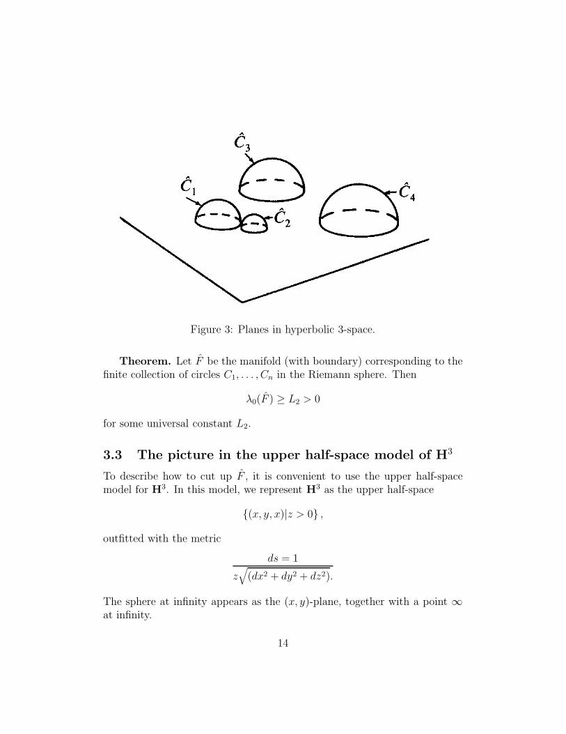
Figure 3: Planes in hyperbolic 3-space.

Theorem. Let F be the manifold (with boundary) corresponding to thefinite collection of circles C1, . . . , Cn in the Riemann sphere. Then

λ0(F ) ≥ L2 > 0

for some universal constant L2.

3.3 The picture in the upper half-space model of H3

To describe how to cut up F , it is convenient to use the upper half-spacemodel for H3. In this model, we represent H3 as the upper half-space

{(x, y, x)|z > 0} ,

outfitted with the metric

ds = 1

z√

(dx2 + dy2 + dz2).

The sphere at infinity appears as the (x, y)-plane, together with a point ∞at infinity.

14

In this model, which was already tacitly used in Figure 3, the circlesC1, . . . , Cn appear as circles, possibly degenerating into straight lines, in the(x, y)-plane. The planes C1, . . . , Cn appear as hemispheres, possibly degen-erating into planes, that are perpendicular to the (x, y)-plane.

3.4 The case of no circles

Suppose first that there are no circles at all (n = 0). Then F is all of H3,and we can make all of our tubes vertical (parallel to the z-axis). The cross-section of the tubes grows exponentially as a function of the length alongthe tube, thanks to the factor of 1

zin the metric: Let dxdy denote the cross-

section of a tube at height 1, that is, where it passes through the surfacez = 1. Then the cross-section at height h is

1

h2dxdy.

But moving from height 1 to height h corresponds to going a distance

d = − log h

along the tube, so the cross-section as a function of distance along the tubeis

e2ddxdy.

Applying the final proposition of section 2, we conclude that

λ0(H3) ≥ 1.

In fact,λ0(H

3) = 1,

so by cutting we haven’t thrown anything away.

3.5 The case of one circle

Suppose that there is only one circle. Moving a point of the circle to ∞ andnormalizing, we may assume that the circle coincides with the x-axis, andthat F is the domain

{(x, y, z)|y ≥ 0, z > 0} .

15

Again, we can cut F into vertical tubes; again, we conclude that

λ0(F ) ≥ 1;

again, the correct answer isλ0(F ) = 1.

3.6 The case of two tangent circles

Suppose that there are two circles that are tangent. Moving the point oftangency to ∞ and normalizing, we may assume that the circles coincidewith the lines y = 0 and y = 1, and that F is the domain

{(x, y, z)|0 ≤ y ≤ 1, z > 0} .

Once again, we can cut into vertical tubes, etc.

3.7 The case of two non-tangent circles

It may seem that we have gone as far as we can go with vertical tubes, butthis isn’t quite true. Suppose that there are two circles C1 and C2 that aren’ttangent. Pick a point on C1, move it to∞, and normalize as in the one-circlecase above. C2 is a bona fide circle in the half-plane

{(x, y)|y ≥ 0} .

Now construct a circle C3 between C1 and C2 that is tangent to C1 and C2.(See Figure 4.) Decompose F into the part F (C1, C3) between C1 and C3,and the part F (C2, C3) between C2 and C3. If we move the point of tangencyof C1 and C3 to∞, we can cut F (C1, C3) into vertical tubes. Similarly, if wemove the point of tangency of C2 and C3 to ∞, we can cut F (C2, C3) intovertical tubes. As for the boundary between F (C1, C3) and F (C2, C3), wecan simply ignore it, since it has measure 0. In this way, we get a cuttingof F into tubes, some of which are vertical from one point of view and somefrom another. Once again, we conclude that

λ0(F ) ≥ 1,

whereas in factλ0(F ) = 1.

16

Figure 4: Introducing a third circle.

Taking a second look at the argument we have just gone through, we seethat it can be simplified as follows: Cut F into the two pieces F (C1, C3) andF (C2, C3). We already know that

λ0(F (C1, C3)) ≥ 1

andλ0(F (C2, C3)) ≥ 1.

By the cutting law,

λ0(F ) ≥ λ0(F (C1, C3) ∪ fromdisjointF (C2, C3))

= min(

λ0(F (C1, C3)), λ0(F (C2, C3)))

≥ 1.

3.8 The case of three or more circles

From now on we will assume that there are three or more circles. We canassume that some pair of circles are tangent: If not, pick one of the circles

17

Figure 5: Normalized configuration.

(say C1) and enlarge it until it hits another of the circles. Call the enlargedcircle C′1, and cut F into the two pieces

F (C1, C′1)

andF (C′1, C2, . . . , Cn).

By the cutting law,

λ0(F ) ≥ min(

λ0(F (C1, C′1)), λ0(F (C′1, C2, . . . , Cn)))

≥ min(

1, λ0(F (C′1, C2, . . . , Cn)))

.

Hence it suffices to find a lower bound for

λ0(F (C′1, C2, . . . , Cn)).

The argument we just went through shows that without loss of generality,we may assume that C1 and C2 are tangent. Moving the point of tangencyto ∞ and normalizing, we may assume that C1 and C2 are the lines y = 0and y = 1. (See Figure 5.)

18

3.9 The obvious strategy doesn’t work

Take a look at the domain F . It lies above the (x, y)-plane, between theplanes y = 0 and y = 1, and on or above the hemispheres C3, . . . , Cn. (Fromnow on, all geometrical terms used will be Euclidean by default.)

How shall we cut this space into tubes? The obvious thing is to startby cutting the space apart along the cylinders that lie above the circlesC3, . . . , Cn. This yields n − 2 domains that are congruent from the hyper-bolic point of view, along with a residual piece. The residual piece can becut into vertical tubes, so all we have to do is show how to cut the hyper-bolically congruent domains into tubes that grow more or less exponentially.Unfortunately, this can’t be done; the bottom of the spectrum of one of thesedomains is 0. The problem is that the intersection of one of these domainswith the plane z = ε has Euclidean area on the order of ε2, hence hyperbolicarea on the order of ε2/ε2 = 1. (See Figure 6.) Since there isn’t an exponen-tial room at infinity, there is no way to cut the domain into tubes that growexponentially.

Notice that in higher dimension, the difficulty we have just encountereddisappears. In the upper half-space model of H4, the Euclidean measure ofthe intersection of an analogous domain with the hyperplane at height ε isstill on the order of ε2, only now the hyperbolic measure is ε2/ε3 = 1/ε. Thusthere is plenty of room at infinity, and it is a simple matter to construct anappropriate cutting into tubes.

Back in H3, we recognize that because of the difficulty we have justdiscussed, we must allow at least some of the tubes that begin over a givenhemisphere to spread out beyond the corresponding circle. In so doing, theywill most likely stray out over other hemispheres, and confusion is liable toresult. Our task will be to avoid this confusion.

3.10 Keeping the tubes more or less vertical

Our strategy for laying out the tubes will be to make them all drop downmore or less vertically toward the (x, y)-plane. To get started, we will makeall of the tubes vertical above height z = 1. (See Figure 7.) This is okaybecause all of the circles have radius ≤ 1/2, so no hemisphere protrudes abovez = 1/2. Below z = 1, we will be forced to bend the tubes. In so doing,we would like to make sure that the tubes stay more or less vertical, in the

19

Figure 6: No room at infinity.

20

Figure 7: Cutting vertically down to height 1.

sense that the angle that the tubes make with the vertical stays boundedabove by some universal constant <π

2. This way, the true cross-section of a

tube will be more or less the same as its horizontal cross-section, that is, thearea of its intersection with the plane z = const. Similarly, the length (eitherhyperbolic or Euclidean) of a section of tube will be more or less the same asthat of its projection onto the z-axis. Thus, instead of worrying about thegrowth of the cross-section as a function of length along the tube, we canworry about the growth of the horizontal cross-section as a function of heightabove the (x, y)-plane. In particular, if we can arrange things so that thetubes stay more or less vertical, and so that the horizontal cross-section ofevery tube never decreases, and increases by a definite factor every time thevertical distance to the (x, y)-plane drops by a factor of 2 (or 8, or whatever),then the tubes will be growing more or less exponentially.

Of course near the tops of the hemispheres there is no way to keep thetubes more or less vertical. This is a real nuisance. To get around thisdifficulty, we will outfit each hemisphere with a duncecap, as shown in Figure8. A hemisphere of radius a gets a cap whose apex is at height z = 2a and

21

Figure 8: Duncecap dimensions.

whose brim rests along the parallel at height z = a/2. Call the region lyingon or above the spruced-up hemispheres G. If we can cut G up into tubesthat grow more or less exponentially, then the same goes for F . (See Figure9.) One way to see this is to consider that the obvious “squash the hats” mapfrom G to F taking (x, y, z) to (x, y, z− f(x, y)) is a quasi-isometry from thepoint of view of the hyperbolic metric. So from now on we will concentrateon cutting up G, rather than F .

3.11 Working our way down

In extending the tubes down toward the (x, y)-plane, we will proceed onestep at a time. On the first step, we will go from height 1 to height 1/2, onthe second step we will go from height 1/2 to height 1/4, etc. On the kthstep we go from height h = 1/2k−1 down to height h/2 = 1/2k. As we dothis, we will only need to consider hemispheres of radius > h/4, since theseare the only ones that protrude into the region we are cutting up. So let usdefine the relevant hemispheres to be those hemispheres (other then C1 andC2) whose radius is > h/4. (See Figure 10.) Note that we do not considera hemisphere relevant if its radius is exactly h/4, so that the apex of its hatis at height exactly h/2. Of course which hemispheres are relevant dependson which step we’re working on.

22

Figure 9: Duncecaps.

23

Figure 10: Relevant hemispheres.

24

It is precisely because we only have to consider big hemispheres thatthis one-step-at-a-time approach will allow us to avoid the confusion that weanticipated from sending tubes starting above one hemisphere out over otherhemispheres. There may well be other hemispheres beneath where we sendour tubes, but they’re irrelevant because they’re small and don’t get in theway. When we’re down so that our distance to the plane is comparable totheir radius, then we’ll worry about those little hemispheres.

3.12 Associating pieces of the plane to relevant hemi-

spheres

In going from height h down to height h/2, we proceed by dividing the (x, y)-plane into pieces, one for each relevant hemisphere, together with a residualpiece. We consider each piece separately: The tubes that begin over a pieceremain over that same piece throughout this stage of their descent. This isprecisely what we tried to do before, only now the piece we associate to eachhemisphere extends beyond the base of the hemisphere, and the hemisphereswe have to consider and the pieces we associate to them change at each step.As before, we will make the tubes vertical over the residual piece. What wehave to figure out is how to associate a piece to each relevant hemisphere,and how to cut up the space above it. Of course these two problems arereally the same: What piece we associate to a hemisphere depends on howwe plan to cut up the space above it.

3.13 Taking care of the babies

Among the relevant hemispheres, we will distinguish those whose hats in-tersect the region we are trying to cut up, i.e. whose radius is ≤ 2h, andrefer to them as babies. Each hemisphere spends three steps as a baby: Ifthe radius is a, the hemisphere will be a baby when h/4 < a ≤ h/2, whenh/2 < a ≤ h, and when h < a ≤ 2h. During each of these steps, the pieceof the (x, y)-plane that we associate to the hemisphere will consist of thebase of the hemisphere, and no more. By deflecting the tubes radially, wecan arrange things so that the tubes stay more or less vertical, and so thatthe horizontal cross-section of every tube never decreases, and increases bya definite factor between the beginning of the first step and the end of thethird. (Look back at Figure 9.) This takes care of the babies.

25

3.14 Room to grow

Consider a hemisphere C, associated to the circle C and the disk D. Let theradius of C be a. We assume that C is relevant, and not a baby, that is, thata > 2h. At height h, the tubes trapped over C cover an annulus A(h) in theplane of outer radius a and inner radius

√a2 − h2. (See Figure 11.) The

Euclidean area of A(h) is

πa2 − π(a2 − h2) = πh2.

This annulus is the image under projection into the plane of the annulus A(h)consisting the intersection of the plane z = h with the locus of points aboveC and inside the cylinder over C. Earlier we determined that the hyperbolicarea of A(h) was on the order of 1. Now we see that it is exactly pi.

In order to insure that the tubes over C have enough room to grow, wewill need to annex around the base of the hemisphere a region B havingEuclidean area on the order of that of A(h), that is, we must have

Area(B) ≥ K ·Area(A(h)) = K · πh2

for some universal constant K. To see that this is the right condition, letB(h) be the portion of the plane z = h that lies over B. The hyperbolic areaof A(h) ∪ B(h) is

1

h2(πh2 + Area(B)) = π + Area(B)h2 ,

while the hyperbolic area of A(h/2) ∪ B(h/2) is

1

(h/2)2(π(h/2)2 + Area(B)) = π + 4Area(B)h2 .

Our assumption on the area of B guarantees that the ratio of the latterquantity to the former will always be ≥1+4K

1+K. Thus in going from height h

down to height h/2 the hyperbolic area available to the tubes increases by adefinite factor, which is the kind of condition we need.

26

Figure 11: No room at infinity reprise.27

Figure 12: Disputed territory.

3.15 Annexing annuli

Of course this condition on the area of the annexed region B is not in itselfenough: It matters how the annexed territory is distributed around C, be-cause all of the tubes have to keep on expanding more or less exponentially,and it might not be possible to avoid pinching tubes over one part of thehemisphere even though there is plenty of extra room somewhere around onthe far side of the hemisphere.

To make sure that the territory we annex is nicely distributed, the idealthing would be to annex an annulus, since then we could just divert our tubesradially away from the center of C, and all would be well. Unfortunately, ifC is tangent or nearly tangent to the base of another relevant hemisphere,or to C1 or C2, hostilities will arise when we try to annex territory belongingto or coveted by the other hemisphere. (See Figure 12.)

28

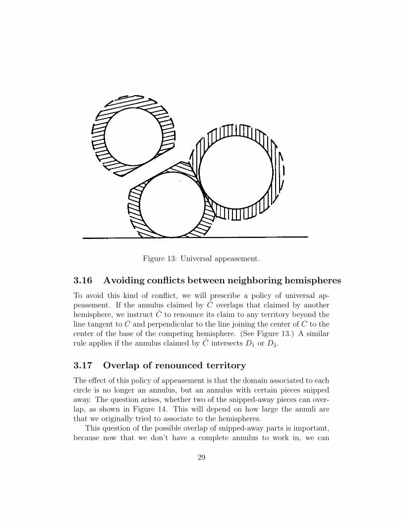
Figure 13: Universal appeasement.

3.16 Avoiding conflicts between neighboring hemispheres

To avoid this kind of conflict, we will prescribe a policy of universal ap-peasement. If the annulus claimed by C overlaps that claimed by anotherhemisphere, we instruct C to renounce its claim to any territory beyond theline tangent to C and perpendicular to the line joining the center of C to thecenter of the base of the competing hemisphere. (See Figure 13.) A similarrule applies if the annulus claimed by C intersects D1 or D2.

3.17 Overlap of renounced territory

The effect of this policy of appeasement is that the domain associated to eachcircle is no longer an annulus, but an annulus with certain pieces snippedaway. The question arises, whether two of the snipped-away pieces can over-lap, as shown in Figure 14. This will depend on how large the annuli arethat we originally tried to associate to the hemispheres.

This question of the possible overlap of snipped-away parts is important,because now that we don’t have a complete annulus to work in, we can

29

Figure 14: Overlap.

30

no longer simply spread our tubes out radially away from the center of thehemisphere. If we do this, the tubes near the middle of the snipped-awaypart will not be growing. If these tubes are to grow, we must allow themto expand laterally, which will squeeze tubes out away from the middle ofthe snipped-away part. (Peek ahead at Figure 24.) But if two snipped-awayparts overlap, there will be nowhere for the tubes to spread out into. Wewant to arrange things so that snipped-away parts can never overlap.

3.18 Avoiding overlap

It turns out that to insure that snipped-away parts don’t overlap, it is suf-ficient to make sure that the annuli that the hemispheres try to annex aresufficiently small, though of course we must still make them large enough tobe useful. Specifically, say that to the hemisphere C, with notation as above,we associate an annulus of outer radius

√a2 + Kh2 ∼ a + Kh2/2a,

where K is some universal constant yet to be specified. The claim is that ifK is chosen small enough, then no two snipped-away parts will ever overlap.The truth of this statement depends on only the grossest of estimates of howdensely one can pack circles in the plane.

3.19 An elementary geometric lemma

Lemma. Let C0, C1, C2 be three circles bounding disjoint open disks in theplane. (See Figure 15.) Let the radii of these circles be a0, a1, a2. Assumethat

a0, a1, a2 ≥ 1.

Let p1 and p2 denote the points on C0 closest to C1 and C2. Let

d0,1 = dist(C0, C1) = dist(p1, C1)

andd0,2 = dist(C0, C2) = dist(p2, C2).

Then for universal constants K1, K2, if

d0,1, d0,2 ≤ K1

31

Figure 15: Notation for the elementary geometric lemma.

32

Figure 16: Special configurations

thendist(p1, p2) ≥ K2.

This proposition remains true in the limit when one or both of the circles C1

and C2 are allowed to degenerate into lines (circles of infinite radius).Proof. Choose any K1 between 0 and 1. Call a configuration of circles a

K1-configuration ifd0,1, d0,2 ≤ K1.

Clearly dist(p1, p2) is a continuous positive function on the space of K1-configurations. The only way for dist(p1, p2) to approach 0 is for somethingbad to happen as one of the radii a0, a1, a2 approaches 0, but it’s easy to seethat no such bad thing happens. Hence there is some appropriate choice forK2.

More concretely, consider the two special K1-configurations for whicha0 = a1 = a2 = 1, d0,1 = K1, d1,2 = 0, and either d0,2 = 0 or d0,2 = K1. (SeeFigure 16.) An arbitrary K1-configuration can be transformed into one ofthese two special configurations by a sequence of steps that do not increasedist(p1, p2). (Without going into detail, the steps are: make a1 = a2 = 1;assume d0,1 ≥ d0,2; make d0,1 = K1; make d1,2 = 0; either make d0,2 = 0 ormake d0,2 = K1; make a0 = 1.) Setting

K1 = 2√

2− 2 = .8284271247 . . .

and computing dist(p1, p2) for the two special configurations, we find (see

33

Figure 17: The case where K1 = 2√

2− 2.

Figure 17) that we can choose

K2 = min(√

2−√

2, 1√2) = 1√

2= .7071067811 . . . .♣

3.20 How little area to ask for

The elementary geometric lemma tells us how small to make K in order tomake sure that no two snipped-away parts overlap. By choosing

K ≤ K1

9,

we can guarantee that any relevant hemisphere with which C conflicts iswithin a distance K1·h

4of C. (See Figure 18.) Thus by the elementary geo-

metric lemma if two hemispheres both conflict with C the distance betweenthe centers of the corresponding snips must be ≥K2·h

4. (Recall that we only

have to worry about relevant hemispheres, which have height >h4

.) But bychoosing

K ≤ K22

64,

34

Figure 18: Making sure conflicting hemispheres are close.

35

we can guarantee that the distance from center to tip of either snip is≤K2

2·h

4.

(See Figure 19.) Thus if the snips overlap, the distance between their centersmust be <K2·h

4, a contradiction.

For the values K1 = 2√

2− 2 and K2=1√2

, we find that these conditions on

K will be satisfied for K=1128

. With this value of K, each hemisphere is askingfor growth room of 1

128th the area that its tubes cover at height h.

3.21 Laying out the tubes

Now we’re in great shape. We have annexed our annulus, and althoughparts have been snipped away, no two snipped-away parts overlap. Withinthe sector defined by one of the snipped-away parts, the annexed area is onthe order of the original area. (See Figure 20.) Thus we hope and expectthat there is enough room for the tubes to grow. To verify this, let us specifyprecisely how the tubes are to run.

The region we are supposed to be cutting up is the portion of G betweenheight h and height h/2 and lying above D ∪B, the union of the base of thehemisphere and the annexed territory. Just as we divided the plane up intopieces, we will divide D∪B into pieces, and treat each such piece separately.We begin by cutting D∪B along the radii that extend to the tips and centersof the snips. (See Figure 21.) This yields pieces of three kinds: sectors,right triangles, and “left triangles.” In discussing how to lay out the tubeswe will ignore left triangles, since they are just like right triangles.

For a given piece S, either a sector or a triangle, let S(z) be the portionof the plane at height z that lies above S, and let

H =⋃

z∈[h/2,h]

S(z).

Our task is to extend the tubes that have run into S(h) down through theregion H until they run into S(h/2). Since the tubes are to remain more orless vertical, this amounts to specifying a correspondence φz between S(h)and S(z) for each z ∈ [h/2, h]. Our strategy is to choose these correcpon-dences so that the available horizontal cross-section is shared equally amongthe tubes, that is, so that

Area(φz(A))

Area(S(z)) = Area(A)

Area(S(h))

36

Figure 19: Making sure snips are short.

37

Figure 20: Comparing areas within a snipped sector.

38

Figure 21: Dividing up D ∪ B.

for all AsubsetS(h).This condition doesn’t determine the φz’s, so we require in addition that

the φz’s be nice and smooth, and take “radii” of S(h) to “radii” of S(z). Tosee what this entails, introduce polar coordinates (r, θ) in the (x, y)-plane sothat the point r = 0 is the center of the disk D and the ray θ = 0 lies just tothe right of S. (See Figure 22.) Then H is determined by the inequalities

h

2 ≤ z ≤ h,

0 ≤ θ ≤ θmax,√a2 − z2 ≤ r ≤ β(θ),

whereβ(θ) =

√a2 + Kh2

when S is a sector, andβ(θ) = a sec θ,

a sec θmax =√

a2 + Kh2

when S is a right triangle. Set

α =√

a2 − z2,

39

Figure 22: Polar coordinates.

40

and define

u =

∫ θ

0β2−α2

2∫ θmax0

β2−α2

2=

∫ θ

0β2−α2

∫ θmax0

β2−α2,

v =

(

r2−α2

2

)

(

β2−α2

2

) =(r2 − α2)

(β2 − α2).

The function u = u(θ, z) tells what fraction of the area of S(z) has θ-coordinate between 0 and θ. The function v = v(r, θ, z) tells what frac-tion of the area of the infinitesimal strip between angles θ and θ + dθ hasr-coordinate between α and r. We make the tubes run along the curvesu = const, v = const. The correspondences φz associate points in S(h) andS(z) that have equal values of u and v. These correspondences are illustratedin Figures 23 and 24. Figure 23 shows a sector; here the tubes are being de-flected radially. Figure 24 shows a right and left triangle together; here inaddition to being deflected radially the tubes are being squeezed from thecenter of the snip out towards the tips.

Have we succeeded in keeping the tubes more or less vertical? This comesdown to checking whether there is a universal upper bound for

(

∂r

∂z

)2

u,v

+ r2

(

∂θ

∂z

)2

u,v

,

where the subscript u, v indicates that u and v are to be held constant.For a sector, this fact is geometrically obvious. For a triangle, this fact is notquite so obvious, but nonetheless true. To see why, consider that the onlyfree parameter is the ratio h/a, and the only way the expression above canfail to be bounded is if something bad happens as h/a goes to 0. So you justhave to convince yourself that nothing bad happens as h/a goes to 0. As alast resort, this can be verified by computation.

3.22 Taking stock

Our task was to cut G into tubes that grow more or less exponentially.To make sure that we have accomplished this, let us follow the course of a

41

Figure 23: Tubes above a sector.

42

Figure 24: Tubes above a pair of triangles.

43

representative tube, as it threads its way down toward the plane. To start off,it drops straight down until it reaches height 1. Below height 1, its journeyis divided into steps of three kinds.

• Steps spent over the residual piece of the plane. In the course of oneof these steps, the tube remains vertical, and its hyperbolic horizontalcross-section grows exponentially.

• Steps spent over a sector or a triangle. In the course of one of thesesteps, the tube remains more or less vertical; its hyperbolic horizontalcross-section does not decrease, and increases by a definite factor fromthe beginning to the end of the step.

• Steps spent taking care of a baby hemisphere. These steps come insets of three. In the course of one of these sets of three steps, thetubes remain more or less vertical; the hyperbolic cross-section doesnot decrease, and increases by a definite factor between the beginningof the first step and the end of the third step.

Taken together, these facts imply that we have indeed succeeded in cut-ting G into tubes that grow more or less exponentially, with rate boundedbelow and factor bounded above by universal constants. But as we remarkedbefore, this implies that we can do the same for the fundamental region F ,so there is a universal lower bound for λ0(F ), and hence for λ0(H

3/Γ). qed

3.23 What is the constant?

In the proof we have just gone through, we neglected to determine precisevalues for various “universal constants.” As a result, while we now know thatthere is a universal lower bound L2 for λ0(F ), and hence a universal upperbound U2 for δ(Γ), we do not know concrete values for these bounds. Withsufficient patience, we could work out precise bounds. However, the resultingbounds are liable to be exceedingly poor. To get good bounds by the cuttingmethod, a keener knife and a steadier hand will be needed.

44

Acknowledgements

I would like to thank Ralph Phillips, Peter Sarnak and Bob Brooks for tellingme about this problem, and their ideas on how to solve it. They also madehelpful comments on earlier versions of this paper, as did Curt McMullen.The referee filled me in on the history of the problem, and supplied some ofthe references cited in the Introduction.

Most of all, I would like to thank Dennis Sullivan for advice and encour-agement.

References

[1] T. Akaza. Poincare theta-series and singular sets of Schottky groups.Nagoya Math. J., 24:43–65, 1964.

[2] T. Akaza. (3/2)-dimensional measure of singular sets of some Kleiniangroups. J. Math. Soc. Japan, 24:448–464, 1972.

[3] R. Brooks. On the deformation theory of classical Schottky groups.Duke Math. J., 52:1009–1024, 1985.

[4] R. Brooks. The spectral geometry of the Apollonian packing. Comm.

Pure Appl. Math., 38:357–366, 1985.

[5] W. Burnside. On a class of automorphic functions. Proc. London Math.

Soc., 23:49–88, 1891.

[6] P. G. Doyle and J. L. Snell. Random Walks and Electric Networks.Mathematical Association of America, Washington, D. C., 1984.

[7] C. J. Holland. A minimum principle for the principal eigenvalue forsecond-order linear elliptic equations with natural boundary conditions.Comm. Pure Appl. Math., 31:509–519, 1978.

[8] J. C. Maxwell. Treatise on Electricity and Magnetism. Clarendon, Ox-ford, third edition, 1891.

[9] P. J. Myrberg. Zur Theorie der Konvergenz der Poincareschen Reihen.Ann. Acad. Sci. Fenn. Ser. A, 9:1–75, 1916.

45

[10] P. J. Myrberg. Zur Theorie der Konvergenz der Poincareschen Reihen(zweite abh.). Ann. Acad. Sci. Fenn. Ser. A, 11:1–29, 1917.

[11] S. J. Patterson. The limit set of a Fuchsian group. Acta Math., 136:241–273, 1976.

[12] S. J. Patterson. Some examples of Fuchsian groups. Proc. London Math.

Soc., 39:276–298, 1979.

[13] R. Phillips and P. Sarnak. The Laplacian for domains in hyperbolicspace and limit sets of Kleinian groups. Acta Math., 155:173–241, 1985.

[14] J. W. S. Rayleigh. On the theory of resonance. In Collected scien-

tific papers, volume 1, pages 33–75. Cambridge Univ. Press, Cambridge,1899.

[15] P. Sarnak. Domains in hyperbolic space and limit sets of Kleiniangroups. In I. W. Knowles and R. T. Lewis, editors, Differential Equa-

tions, pages 485–500. North-Holland, Amsterdam, 1984.

[16] F. Schottky. Uber eine specielle Function, welche bei einer bestimmtenlinearen Transformation ihres Argumentes unverandert bleibt. Crelle’s

J., 101:227–272, 1887.

[17] D. Sullivan. Discrete conformal groups and measurable dynamics. Bull.

Amer. Math. Soc., 6:57–73, 1982.

[18] D. Sullivan. Entropy, Hausdorff measures old and new, and the limitsets of geometrically finite Kleinian groups. Acta Math., 153:259–277,1983.

46