arX

iv:2

007.

0424

0v1

[ph

ysic

s.fl

u-dy

n] 8

Jul

202

0

On the application of simplified rheological models of fluid in the

hydraulic fracture problems∗

Michal Wrobel

Department of Civil and Environmental Engineering, University of Cyprus,

75 Kallipoleos Street, 1678 Nicosia, Cyprus

wrobel.michal@ucy.ac.cy

Abstract

In this paper we analyse a problem of a hydraulic fracture driven by a non-Newtonian shear-thinning fluid. For the PKN fracture geometry we consider three different rheological models offluid: i) the Carreau fluid, ii) the truncated power-law fluid, iii) the power-law fluid. For each ofthese models a number of simulations are performed. The results are post-processed and comparedwith each other in order to find decisive factors for similarities/dissimilarities. It is shown thatunder certain conditions even the basic power-law rheology can be a good substitute for the Carreaucharacteristics. Although for a particular fluid such a conclusion cannot be made a priori, post-processing based on average values of the fluid shear rates is a very good tool to verify credibilityof the results obtained for simplified rheological models. The truncated power-law rheology is agood alternative for the Carreau model. It always produces results that are very similar to thoseobtained with the equivalent Carreau fluid and simultaneously provides a relative ease of numericalimplementation.

Keywords: hydraulic fracture, shear-thinning fluid, Carreau fluid

1 Introduction

The phenomenon of hydraulic fracture (HF) is encountered in many natural and man-made processes. One of itsmost prominent applications is fracking technology used to stimulate hydrocarbon reservoirs. The highly mul-tiphysical nature of the underlying physical mechanism necessitates careful analysis of the interactions betweenrespective component physical fields in order to properly predict evolution of hydraulically induced fractures andoptimally design the treatments.

The hydraulic fracturing process is influenced essentially by rheological properties of the fracturing fluid. De-pending on the geology of formation, economic factors, stage and overall scenario of the treatment, the fracturingfluids are engineered accordingly so as to achieve optimal combination of chemical and mechanical properties.There are many requirements that involve physical behaviour of fracturing fluids. One can mention amongthem (Barbati et al., 2016): i) viscosity sufficient to create desirable fracture width, ii) suspending propertiesthat facilitate proppant transport under both dynamic and static conditions and mitigate the risk of bridgingphenomenon (Garagash et al., 2019), iii) low leak-off to formation, iv) short time of fracture closure after theinflux shut-off to prevent proppant settling, and others. Moreover, the desired properties should be retained overspecific temperature ranges and chemical environments. No wonder, all these needs can hardly be addressedby any Newtonian fluid. For this reason complex fluids have been widely employed in the oilfield industry. Asthe shear-thinning rheology improves suspending properties of the fluid, many fracturing fluids are intentionallymade shear-thinning (e.g. by adding polymers (Bao et al., 2017)).

∗Preprint submitted to International Journal of Engineering Science

1

In fact, rheology of numerous fracturing fluids yields shear-thinning behaviour only over some limited rangeof shear rates. At low shear rates a Newtonian plateau is observed for which the apparent viscosity achievesa maximum. It is only above a critical value of shear rate that the fluid shear thins. Similarly, at very highshear rates the viscosity reaches another Newtonian plateau corresponding to that of the base solvent used(Moukhtari & Lecampion, 2018). It is still not well recognised how the viscosity plateaus and the shear-thinningamplitude affect the propagation of hydraulic fractures.

Such a complex behaviour of a fracturing fluid can be well reproduced by four parameter rheological modelse.g. Carreau or Cross (Bird, 1987). Unfortunately, when using these models respective flow equations cannot beintegrated analytically to obtain expressions for the fluid velocity and the fluid flow rate in the form used routinelyfor the hydraulic fracture problem in the framework of lubrication theory. Instead a power-law rheology is usuallyemployed (Adachi & Detournay, 2002; Garagash, 2006; Peck et al., 2018,a) which enables a derivation of thePoiseulle-type relation for the fluid flow rate. Moreover, in petroleum industry it is customary to sample only alimited viscosity data, in a narrow shear rate range (typically 25 1

sto 100 1

s), in order to find fitting parameters

for the averaged power-law characteristics (Huang & Desroches, 2004). Naturally, such an oversimplified modelcannot correctly describe the beahviour of fracturing fluid in a broad range of shear rates. Considering asubstantial gradation of the shear rate values along the fracture length it is evident that the pure power-lawmodel does not reflect properly the near-tip high shear rate behaviour of the fluid and, depending on theprocess parameters, can largely overestimate the viscosity in the proximity of the crack mouth. Furthermore,when the hydraulic fracture model accounts for the hydraulically induced tangential tractions on the crack faces(Wrobel et al., 2017, 2018), the elasticity equation cannot be asymptotically balanced near the fracture tip forthe power-law rheology.

A study on the near-tip behaviour of a hydraulic fracture driven by Carreau fluid was conducted in Moukhtari & Lecampion(2018) where the authors analysed a problem of a semi-infinite plane strain crack propagating at a constantspeed in an impermeable material. Quantification of influence of the fracturing fluid rheology on the fluid lagwas performed. Nevertheless, a problem of a finite hydraulic fracture and its temporal evolution still needs tobe addressed. A question whether the frequently used power-law rheology can be an acceptable substitute forthe Carreau-like model is yet to be answered. Some indication on the significance of this issue can be found inHuang & Desroches (2004) where the authors investigate the hydraulic fracture problem for a fluid with a singleshear stress plateau assuming the PKN fracture geometry (Nordgren, 1972). A piecewise power-law model isintroduced to describe the fluid rheology. The authors conclude that the conventional power-law model may beinadequate for accurate prediction of the fracture geometry.

In Lavrov (2015) a concept of truncated power-law fluid was used to analyse the velocity profiles and fluidflow rates in a slit flow (thin flat channel). The truncated power-law rheology, being a four-parameter model,constitutes a simple regularisation of the power-law model, where cut-off viscosities are introduced for the highand low shear rates. In this way, the truncated power-law model can reproduce correctly the limiting behaviourof the Carreau or Cross fluid with the interim power-law approximation of the Carreu/Cross characteristics. Theanalysis presented in Lavrov (2015) shows that the truncated power-law rheology eliminates inherent drawbacksof the power-law model, producing results that are much closer to those obtained for the Carreau fluid even inthe low and high shear rate ranges. However, a question whether such an approximation is sufficient for thehydraulic fracturing problems still remains open.

An efficient algorithm for numerical computation of the velocity profiles and fluid flow rates for a class ofgeneralised Newtonian fluids (Bird, 1987) was introduced in Wrobel (2019). The computational scheme assumespiecewise approximation of the apparent viscosity with subsequent analytical integration of the resulting flowequations. Using the example of a slit flow the author showed that the algorithm can provide any desirableaccuracy of solution at a computational cost that is only a fraction of those produced by other schemes availablein the literature. As such, the new algorithm can be a numerical substitute of the Poiseulle-type relation in thehydraulic fracture problems.

In this paper we address a problem of a hydraulic fracture driven by a shear-thinning fluid. For the analysiswe assume the PKN fracture geometry. The algorithm from Wrobel (2019) is adapted to compute the fluid flowrates in the case of fracture of elliptic cross section. This subroutine is integrated with the hydraulic fracturesolver developed in Wrobel & Mishuris (2015); Perkowska et al. (2016). A number of simulations are performedfor three different rheological models of fluids: i) the Carreau model, ii) the truncated power-law model, iii) thepower-law model. Based on the numerical results we verify whether and under what conditions the simplifiedrheologies can be considered credible substitute for the Carreau law.

2

The paper is structured as follows. In Section 2 we introduce general relations for the hydraulic fractureproblem of the PKN geometry. Section 3 includes constitutive relations for respective rheological models offluid together with corresponding expressions for the fluid flow rates. Computational relations for the Carreauvariant are derived in Appendix A. In Section 4 we perform a number of simulations for four different fracturingfluids. Each of these fluids is described by all three analysed rheologies. A discussion on the numerical results isprovided in Section 5. Final conclusions are given in Section 6.

2 General relations

Let us consider a hydraulic fracture whose geometry is defined by the classical PKN model (Nordgren, 1972).The symmetrical two-winged fracture of length 2L propagates in the plane x ∈ [−L, L], where L = L(t). In thefollowing we analyse only one of the symmetrical parts, i.e. x ∈ [0, L], as shown in Fig. 1. The fracture height,H , is assumed constant, while the fracture opening, w(x, t), depends on the net fluid pressure, p(x, t), and is anelement of the solution. The relation between p and w is of the following form:

p(x, t) = kw(x, t), (1)

where k = E2(1−ν2)H

, with E and ν being the Young modulus and the Poisson’s ratio, respectively. The mass

conservation principle expressed by the continuity equation yields:

∂w

∂t+

∂q

∂x+ ql = 0, (2)

where q(x, t) is the normalised fluid flow rate through the fracture cross sections and ql(x, t) stands for thenormalised leak-off function (both quantities use a normalisation factor: Hπ/4 - compare e.g. Nordgren (1972)).The fluid velocity averaged over the fracture cross section is defined as:

v =q

w. (3)

We assume that there is no lag between the fluid front and the fracture tip and the leak-off is bounded at thecrack apex, which implies:

v(L, t) =dL

dt. (4)

Respective boundary conditions for the problem include:

• two tip boundary conditions:w(L, t) = 0, q(L, t) = 0, (5)

• the influx boundary condition:q(0, t) = q0(t). (6)

Finally, the initial conditions define the initial crack length and the initial fracture aperture:

L(0) = L∗, w(x, 0) = w∗(x). (7)

3 Fluid flow equations

In the paper we compare results obtained for three rheological models of fluids: i) the power-law fluid, ii) theCarreau fluid, ii) the truncated power-law fluid, each of them complying with a definition of the generalisedNewtonian fluid. Respective equations for the fluid flow rate, that supplement the problem formulation from theprevious section, are given below.

3

flowdirec

tion

z

x

y

w(x, t)

H

L(t)

Figure 1: The PKN fracture geometry. Only one of the fracture wings is shown. Velocity profile in thecross section z = 0 is marked by red arrows.

3.1 Power-law model

The simplest model that can describe a non-Newtonian behaviour of a fluid is the power-law model (Bird, 1987;Gholipour et al., 2018) for which the apparent viscosity is expressed as:

ηa = C|γ̇|n−1, (8)

where C is the consistency index, n stands for the fluid behaviour index, while γ̇ denotes the shear rate. For n < 1it reflects the shear-thinning properties, while n > 1 produces the shear-thickening characteristic. Unfortunately,this model yields unphysical results for low and high shear rates. In the case of shear-thinning behaviour oneobtains infinite viscosity for zero shear rate and zero viscosity as γ̇ → ∞. For the shear-thickening variant areverse trend holds. The big advantage of the power-law model is that it enables analytical integration of therespective flow equations to obtain expression for the average fluid flow rate. For the elliptical channel in thePKN model the respective normalisedfluid flux is given by the formula (see Remark 1 in Appendix A):

q =n

1 + 3n2−

n+1n

(

−1

C

∂p

∂xw2n+1

)1/n

. (9)

3.2 Carreau model

We employ the model of Carreau-Yasuda fluid (Habibpour & Clark, 2017) whose apparent viscosity can bedescribed by the following relation:

η(c)a = η∞ + (η0 − η∞) [1 + |λγ̇|a]

n−1a , (10)

η0 is the viscosity at zero shear rate, η∞ is the limiting viscosity for γ̇ → ∞, while λ, a and n are fittingparameters. The Carreau-Yasuda model has been recognised to imitate well the physical behaviour of many

4

fracturing fluids (Moukhtari & Lecampion, 2018). It eliminates the inherent deficiency of the classical power-lawmodel described above. Unfortunately, expression (10) does not allow analytical integration of the respectivefluid flow equations to obtain an average fluid flow rate even in the conduits of simple geometries.

In Wrobel (2019) a numerical scheme was proposed that enables effective computation of the velocity andfluid flow rates for the generalised Newtonian fluids in conduits of simple geometries. It was shown that theprocedure can be successfully used as a numerical substitute for the Poiseulle-type relation for q. The schemeassumes piecewise approximation of the apparent viscosity in the form:

ηa =

η0 for |γ̇| < |γ̇1|,

Cj |γ̇|nj−1 for |γ̇j | < |γ̇| < |γ̇j+1| j = 1, ..., N − 1,

η∞ for |γ̇| > |γ̇N |,

(11)

where the values of γ̇j , Cj and nj are taken in a way to preserve continuity of ηa and provide the best approxi-mation of the original rheological law for the chosen value of N . A method to construct approximation (11) isgiven in Wrobel (2019).

In Appendix A we extend the algorithm from Wrobel (2019), originally proposed for the slit flow, to the caseof an elliptic channel for the PKN geometry. The corresponding expressions for q are (41) - (46). Note that thefluid flow rate computed in this way takes into account full velocity profile across the channel height.

As explained in Appendix A, when analysing the flow in the elliptic cross section of the channel for theviscosity model (11) one can distinguish up to N + 1 shear rate layers in each of the symmetrical parts of theconduit (see Fig. 24). Among them there are: i) a Newtonian type layer of viscosity η0 at the core of the flow -its thickness in the plane z = 0, δ1, is given by formula (35), ii) N −1 power-law layers of thicknesses (z = 0), δj ,defined by (36), iii) a Newtonian layer with viscosity η∞ adjacent to the channel wall whose thickness (z = 0),δN+1, is described by (37). Comparing the total thickness of the latter Newtonian layer, 2δN+1, with the overallfracture opening, w, we obtain:

2δN+1

w= 1−

N∑

i=1

2δiw

. (12)

Now, let us recall that:

δi ∝

(

−∂p

∂x

)

−1

, i = 1, ..., N. (13)

When approaching the fracture tip the pressure gradient tends to −∞. Thus, the thicknesses of respective layerstend to zero. For the standard estimation of the crack tip asymptotics:

w ∝ (L− x)α, x → L,

we have that:δjw

∝ (L− x)1−2α, x → L, i = 1, ..., N. (14)

In this way, for any permissible value of α for the shear-thinning fluids in the PKN model (1/3 ≤ α < 1/2 - seee.g. Perkowska et al. (2016)) the following estimations are satisfied:

δjw

→ 0, x → L, i = 1, ..., N, (15)

2δN+1

w→ 1, x → L. (16)

As can be seen, in the immediate vicinity of the fracture tip the high shear rate Newtonian layer of viscosityη∞ tends to occupy the whole width of the fracture. Thus, over at least some small distance behind the crackfront the fracturing fluid behaves like a Newtonian fluid of viscosity η∞.

Having the above feature in mind, we introduce in our analysis the following formulation of the fluid flowrate:

q = −1

16η∞w3 ∂p

∂xF (x, t) , (17)

where:

F (x, t) = −128η∞w4

(

∂p

∂x

)

−1 ∫ w/2

0

yV dy. (18)

5

The integral on the right hand side of (18) is computed according to formulae (42)-(46) for V being the fluidvelocity profile in the plane z = 0 (see Appendix A). Note that for the purely Newtonian regime of flow withviscosity η∞ function F assumes a unit value, while for the Newtonian flow at low shear rates with viscosity η0F yields η∞/η0. In particular, when taking into account (16), one has:

F → 1, x → L(t). (19)

Thus, F (x, t) informs us to what degree the solution in a certain spatial and temporal location deviates from thehigh shear rate Newtonian regime of flow. As such, this function can be very instructive in understanding theunderlying flow phenomena and it will be used in our analysis.

3.3 Truncated power-law model

The truncated power-law model constitutes a simple regularization of the pure power-law model, where lowand high shear rate cut-off viscosities, η0 and η∞, are introduced. As such it can be considered a special caseof approximation (11) for N = 2. This time, up to three shear rate layers can appear within each of thechannel symmetrical parts, with two of them being Newtonian-type layers of viscosities η0 and η∞, respectively.Consequently, the estimations (15)–(16) hold, which means that in the immediate vicinity of the fracture tip thefluid behaves like a Newtonian fluid of viscosity η∞. For the fluid flow rate, q, in this case we keep representation(17)–(18) with the computational relations (42) - (46) employed.

As shown in Lavrov (2015), the truncated power-law model produces much more reliable results than thepure power-law in terms of fluid velocity and fluid flow rate. However, the presented data suggests that oversome ranges of pressure gradient this approximation may not be sufficient for practical applications. This issuewill be verified in the paper by comparison with results obtained for the Carreau model.

4 The numerical results

In this section we will simulate numerically the process of hydraulic fracture propagation for four different typesof fracturing fluids:

• The fluid described in Lavrov (2015), where the Carreau model parameters and the corresponding truncatedpower-law coefficients are provided. It will henceforth be called fluid 1.

• Hydroxypropylguar (HPG) fluid - the Carreau model parameters are given in Moukhtari & Lecampion(2018).

• Solution of partially hydrolyzed polyacrylamide (HPAM) with the concentartion of 150 weight parts permillion (wppm) for which the Careau-Yasuda model parameters are available in Habibpour & Clark (2017).

• Xanthan gum (XG) solution of 600 wppm concentration. The Careau-Yasuda model parameters are takenfrom Habibpour & Clark (2017).

The parameters used for the Carreau-Yasuda and the truncated power-law models are collected in Table4. Respective values for the truncated power-law model were taken in a way to minimise the maximal relativedeviation from the Carreau-Yasuda variant (for fluid 1 C and n were adopted directly from Lavrov (2015)). Forthe pure power-law model we use the same parameters (C and n) as for the truncated power-law case.

In order to illustrate the influence of fluid rheology on the overall process we will make comparisons for twopairs of fluids: i) fluid 1 and HPG, ii) 150 wppm HPAM and 600 wppm XG. Note that in each of these pairs thelimiting viscosities (η0 and η∞) are virtually the same. As can be seen in Fig. 2 however, the interim behavioursbetween the viscosity plateaus are different. For the first pair (fluid 1 and HPG) one can observe a very large(a few orders of magnitude in |γ̇|) translation of the ηa characteristics towards the high shear rate values for theHPG fluid. For the second pair similar trend is much less pronounced.

Assuming some typical values of the HF parameters for the PKN model we will investigate to what degreethe aforementioned rheological features affect the fracture evolution and whether the simplified viscosity models(power-law and truncated power-law) can be considered credible substitutes for the original Carreau rheology.Following e.g. Huang & Desroches (2004); Wang et al. (2018) we set: E = 10 GPa, ν = 0.2, H = 20 m,

6

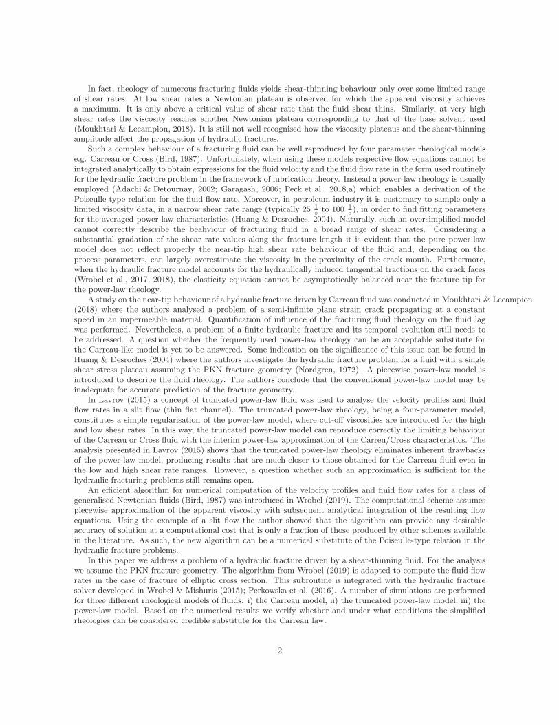
fluidCarreau Truncated power-law

η0, Pa·s η∞, Pa·s λ, s a n C, Pa·sn n |γ̇1|, s−1 |γ̇2|, s

−1

fluid 1 0.5 10−3 600 2 0.25 5 · 10−3 0.3 1.39 · 10−3 9.97HPG 0.44 10−3 0.303 2 0.46 0.464 0.567 1.128 1.45 · 106

150 wppm HPAM 0.2668 4.1 · 10−3 5.46 3.15 0.26 7.27 · 10−2 0.476 8.37 · 10−2 241600 wppm XG 0.2689 4 · 10−3 5.34 1.92 0.43 8.82 · 10−2 0.6 6.17 · 10−2 2283

Table 1: Parameters of the Carreau and the truncated power-law models (for the Carreau model re-spective data was taken from Lavrov (2015), Moukhtari & Lecampion (2018) and Habibpour & Clark(2017)). The limiting viscosities are the same for both models.

10-4 10-2 100 102 104 106 108

10-3

10-2

10-1

100

|γ̇|

ηa

Figure 2: The apparent viscosities, ηa [Pa·s], according to the Carreau-Yasuda model for the analysedfluids. Respective parameters are collected in Table 4.

q0 = 1.5 ·10−4 m2

s(note that for the fluid influx the normalisation (40) holds). The influx magnitude is increased

from zero for t = 0 s to the maximum q0 at t1 = 10 s and then kept constant according to the following formula:

q̄0(t) =

{

(

3t21t2 − 2

t31t3)

q0 t < t1,

q0 for t ≥ t1.(20)

This particular choice of t1 enables observation of fracture evolution under gradual increase of q̄0. The leak-offto the rock formation is neglected (ql = 0) and the initial fracture length and velocity are assumed zero. Theoverall time of the process is set to tend = 3600 [s].

The computations are performed by the HF solver introduced in Wrobel & Mishuris (2015); Perkowska et al.(2016) with some modifications to implement formula (41) instead of the classical Poiseulle-type relation. Thescheme is based on two blocks: i) subroutine computing the fluid velocity from the continuity equation (2), ii)subroutine for the fracture opening utilising elasticity operator (1). For the Carreau-Yasuda models we employapproximation (11) for N = 100 which, according to the analysis conducted in Wrobel (2019), provides theaccuracy of the order 10−5 for both, the apparent viscosity itself and the fluid flow rate.

7

4.1 Fluid 1 and HPG fluid

We start our analysis with the first two fluids from Table 4. The graphs of apparent viscosities, ηa, are shownin Fig. 3a) for the Carreau and the truncated power-law (TPL) rheologies. The quality of approximation of therespective Carreau characteristics by their truncated power-law imitations measured by the relative differences,δηa, are depicted Fig. 3b). We see that for fluid 1 the maximal error of approximation reaches over 40%, whilefor the HPG the highest deviation is below 30%.

10-4 10-2 100 102 104 106 108

10-3

10-2

10-1

100

10-4 10-2 100 102 104 106 108 10100

0.05

0.1

0.15

0.2

0.25

0.3

0.35

0.4

0.45

|γ̇| |γ̇|

a) b)

ηa δηa

Figure 3: Fluid 1 and HPG fluid: a) apparent viscosities for Carreau and truncated power-law (TPL)rheologies, ηa [Pa·s], b) relative deviations between the Carreau and the truncated power-law variants,δηa.

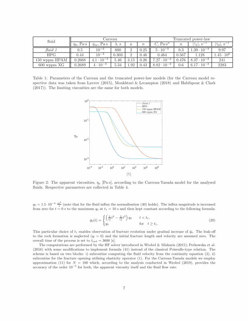
The simulation results for fluid 1 in terms of: i) the fracture length, L, ii) the crack propagation speed, v0,and iii) the fracture opening at the crack mouth, w(0, t), are shown in Figs. 4–5. As can be seen, the resultsobtained for the truncated power-law rheology are almost indistinguishable from those for the Carreau fluid (therelative deviations from the Carreau variant are well below 1% in almost the entire time interval). At the sametime, for the power-law fluid one has huge overestimation of the crack length and the crack propagation speedwith the substantial underestimation of the crack opening. This data suggests that the apparent viscosity offluid obtained for the power-law model is much lower than that achieved with the remaining rheologies.

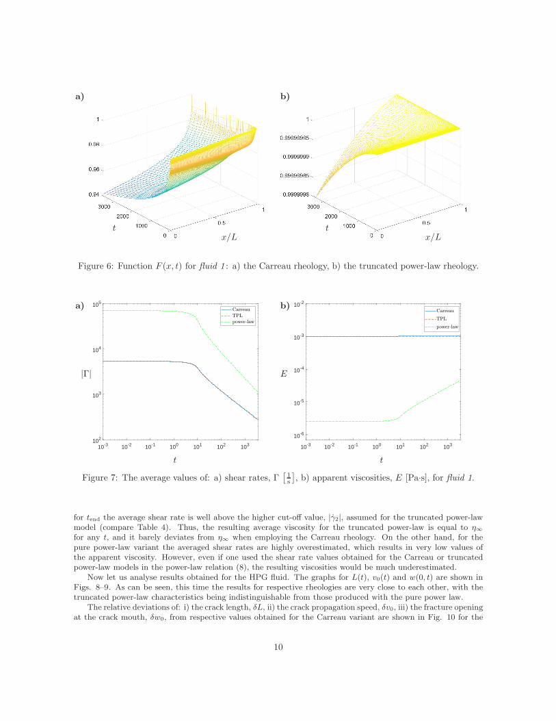
In Fig. 6 we show distributions of the fluid flux component function F (see equations (17)–(19)) over spaceand time for the Carreau and the truncated power-law models. In both cases we see that with time growingthe fracture deviates from the high shear rate Newtonian regime of flow with viscosity η∞. However, in theconsidered time span, this deviation is either very low (Carreau) or virtually negligible (truncated power-law).Thus, we can conclude that within the whole duration of the simulated process the fluid is subjected to the shearrates that are sufficient to yield the apparent viscosity very close to the limiting value η∞.

In order to quantify this trend let us introduce the following parameters:

• The fluid shear rate averaged over fracture cross-section (see Fig. 1 and Fig. 24 for schematic view of theintegration area):

Γ(t) =2

L(t)

∫ L(t)

0

1

w(x, t)

∫w(x,t)

2

0

γ̇(x, y, t)dydx. (21)

The values of shear rate, γ̇, are obtained in post-processing computations. The basic computationalrelation here is equation (34) treated as a non-linear algebraic equation with respect to γ̇. The procedureto compute and integrate the shear rate function is described in Wrobel (2019).

8

0 500 1000 1500 2000 2500 3000 35000

100

200

300

400

500

600

700

800

900

10-3 10-2 10-1 100 101 102 1030

0.2

0.4

0.6

0.8

1

1.2

t t

a) b)

L v0

Figure 4: Simulation results for fluid 1 : a) the crack length, L [m], b) the crack propagation speed, v0[

m

s

]

.

0 500 1000 1500 2000 2500 3000 35000

0.2

0.4

0.6

0.8

1

1.2

1.4

1.6

1.8

210-3

t

w(0, t)

Figure 5: Simulation results for fluid 1 : the fracture opening at the crack mouth, w(0, t) [m].

• The apparent viscosity averaged over fracture cross-section:

E(t) = ηa(Γ), (22)

where formula for ηa is taken according to the respective rheological model.

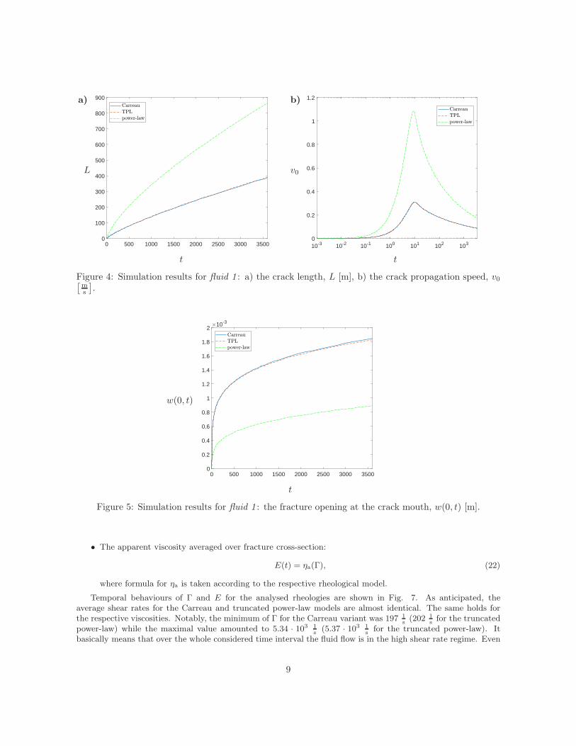
Temporal behaviours of Γ and E for the analysed rheologies are shown in Fig. 7. As anticipated, theaverage shear rates for the Carreau and truncated power-law models are almost identical. The same holds forthe respective viscosities. Notably, the minimum of Γ for the Carreau variant was 197 1

s(202 1

sfor the truncated

power-law) while the maximal value amounted to 5.34 · 103 1s(5.37 · 103 1

sfor the truncated power-law). It

basically means that over the whole considered time interval the fluid flow is in the high shear rate regime. Even

9

tx/L

tx/L

a) b)

Figure 6: Function F (x, t) for fluid 1 : a) the Carreau rheology, b) the truncated power-law rheology.

10-3 10-2 10-1 100 101 102 103102

103

104

105

10-3 10-2 10-1 100 101 102 103

10-6

10-5

10-4

10-3

10-2

t t

a) b)

|Γ| E

Figure 7: The average values of: a) shear rates, Γ[

1

s

]

, b) apparent viscosities, E [Pa·s], for fluid 1.

for tend the average shear rate is well above the higher cut-off value, |γ̇2|, assumed for the truncated power-lawmodel (compare Table 4). Thus, the resulting average viscosity for the truncated power-law is equal to η∞for any t, and it barely deviates from η∞ when employing the Carreau rheology. On the other hand, for thepure power-law variant the averaged shear rates are highly overestimated, which results in very low values ofthe apparent viscosity. However, even if one used the shear rate values obtained for the Carreau or truncatedpower-law models in the power-law relation (8), the resulting viscosities would be much underestimated.

Now let us analyse results obtained for the HPG fluid. The graphs for L(t), v0(t) and w(0, t) are shown inFigs. 8–9. As can be seen, this time the results for respective rheologies are very close to each other, with thetruncated power-law characteristics being indistinguishable from those produced with the pure power law.

The relative deviations of: i) the crack length, δL, ii) the crack propagation speed, δv0, iii) the fracture openingat the crack mouth, δw0, from respective values obtained for the Carreau variant are shown in Fig. 10 for the

10

0 500 1000 1500 2000 2500 3000 35000

20

40

60

80

100

120

140

160

180

10-3 10-2 10-1 100 101 102 1030

0.02

0.04

0.06

0.08

0.1

0.12

0.14

0.16

0.18

0.2

t t

a) b)

L v0

Figure 8: Simulation results for the HPG fluid: a) the crack length, L [m], b) the crack propagationspeed, v0

[

m

s

]

.

0 500 1000 1500 2000 2500 3000 35000

0.5

1

1.5

2

2.5

3

3.5

4

4.510-3

t

w(0, t)

Figure 9: Simulation results for the HPG fluid: the fracture opening at the crack mouth, w(0, t) [m].

truncated power-law and the power-law rheologies. In the analysed time span neither of the shown parametersexceeds 5%, which constitutes a very good approximation of the Carreau solution for practical purposes.

The fluid flux component function, F , is depicted in Fig. 11 for the Carreau and the truncated power-lawmodels. We see that with growing time the fluid flow evolves towards the low shear rate regime. However, unlikethe fluid 1 example, even for small time we are relatively far away from the high shear rate regime. It is onlythe near-tip zone where F grows appreciably.1 This, together with very good coincidence between the resultsobtained for various fluid rheologies, suggests that under the analysed values of the HF process parameters it is

1The employed computational algorithm assumes that the spatial domain is truncated to the dimension x ∈ [0, L(1−ε)]where ε is a regularisation parameter. For this reason the results displayed in Fig. 11 do not cover the small near-tip regionx ∈ [L(1 − ε), L] and thus the limiting value F = 1 at the crack tip is not visible here. In the computations we assumed

11

10-3 10-2 10-1 100 101 102 10310-4

10-3

10-2

10-1

10-3 10-2 10-1 100 101 102 10310-4

10-3

10-2

10-1

t t

a) b)

Figure 10: The relative deviation of solution from the Carreau variant for the HPG fluid in the case of:a) the truncated power-law rheology b) the power-law rheology.

the intermediate (power law) part of the viscosity characteristics that affects final solution the most.

tx/L

tx/L

a) b)

Figure 11: Function F (x, t) for the HPG fluid: a) the Carreau rheology, b) the truncated power-lawrheology.

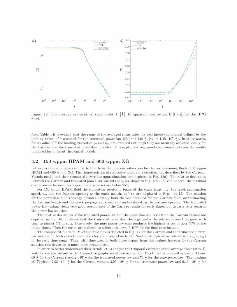
In order to verify this claim we present in Fig. 12 the average values of the fluid shear rate, Γ (21), and theaveraged viscosities, E (22). It shows that the respective shear rate values are very close to each other. Theresulting viscosities are also very similar, especially those obtained for the truncated power-law and the purepower-law. The minima of |Γ| are: 31 1

sfor the Carreau rheology, 32 1

sfor the truncated power-law and 24 1

s

for the pure power-law. The maximal values of |Γ| yield: 1.83 · 103 1sfor the Carreau model, 1.73 · 103 1

sfor

the truncated power-law and 1.76 · 103 1sfor the pure power-law. When comparing the above figures with data

ε = 10−6. For more details on the regularisation technique see Wrobel & Mishuris (2015); Perkowska et al. (2016).

12

10-3 10-2 10-1 100 101 102 103

102

103

10-3 10-2 10-1 100 101 102 1030.01

0.02

0.03

0.04

0.05

0.06

0.07

0.08

0.09

0.1

t t

a) b)

|Γ| E

Figure 12: The average values of: a) shear rates, Γ[

1

s

]

, b) apparent viscosities, E [Pa·s], for the HPGfluid.

from Table 4 it is evident that the range of the averaged shear rates fits well inside the interval defined by thelimiting values of γ̇ assumed for the truncated power-law (|γ̇1| = 1.128 1

s, |γ̇2| = 1.45 · 106 1

s). In other words,

for no value of Γ the limiting viscosities η0 and η∞ are obtained (although they are naturally achieved locally forthe Carreau and the truncated power-law models). This explains a very good coincidence between the resultsproduced for different rheological models.

4.2 150 wppm HPAM and 600 wppm XG

Let us perform an analysis similar to that from the previous subsection for the two remaining fluids: 150 wppmHPAM and 600 wppm XG. The characteristics of respective apparent viscosities, ηa, described by the Carreau-Yasuda model and their truncated power-law approximations are depicted in Fig. 13a). The relative deviationsbetween the Carreau and truncated power-law variants of ηa are shown in Fig. 13b). As can be seen, the maximaldiscrepancies between corresponding viscosities are below 25%.

For 150 wppm HPAM fluid the simulation results in terms of the crack length, L, the crack propagationspeed, v0, and the fracture opening at the crack mouth, w(0, t), are displayed in Figs. 14–15. The solutionfor the power-law fluid rheology deviates notably from the one obtained for the Carreau fluid, overestimatingthe fracture length and the crack propagation speed and underestimating the fracture opening. The truncatedpower-law variant yields very good resemblance of the Carreau results for early times, but departs later towardsthe power-law solution.

The relative deviations of the truncated power-law and the power-law solutions from the Carreau variant aredepicted in Fig. 16. It shows that the truncated power-law rheology yields the relative errors that grow withtime to almost 5% at tend. Conversely, the pure power-law case produces the highest errors of over 50% at theinitial times. Then the errors are reduced to achieve the level 5-10% for the final time instant.

The component function, F , of the fluid flux is depicted in Fig. 17 for the Carreau and the truncated power-law models. In both cases the solutions for q are very close to the Newtonian high shear rate variant (ηa = η∞)in the early time range. Then, with time growth, both fluxes depart from this regime, however for the Carreausolution this deviation is much more pronounced.

In order to better understand these trends let us analyse the temporal evolution of the average shear rates, Γ,and the average viscosities, E. Respective graphs are shown in Fig. 18. This time the minimal values of |Γ| are:69 1

sfor the Carreau rheology, 67 1

sfor the truncated power-law and 73 1

sfor the pure power-law. The maxima

of |Γ| yield: 2.98 · 103 1sfor the Carreau variant, 3.05 · 103 1

sfor the truncated power-law and 6.46 · 103 1

sfor

13

10-2 100 102 104 106

10-2

10-1

10-3 10-1 101 103 105 107 1090

0.05

0.1

0.15

0.2

0.25

|γ̇| |γ̇|

a) b)

ηa δηa

Figure 13: 150 wppm HPAM fluid and 600 wppm XG fluid: a) apparent viscosities for Carreau andtruncated power-law (TPL) rheologies, ηa [Pa·s], b) the relative deviations between the Carreau and thetruncated power-law variants, δηa.

0 500 1000 1500 2000 2500 3000 35000

50

100

150

200

250

300

10-3 10-2 10-1 100 101 102 1030

0.05

0.1

0.15

0.2

0.25

0.3

0.35

t t

a) b)

L v0

Figure 14: Simulation results for the 150 wppm HPAM fluid: a) the crack length, L [m], b) the crackpropagation speed, v0

[

m

s

]

.

the pure power-law. When comparing these figures with the data from Table 4 one concludes that the obtainedaverage shear rates are well above the lower limiting value for the truncated power-law model (|γ̇1| = 8.37 · 10−2

1s). Moreover, they are also above the higher limiting shear rate (|γ̇2| = 241 1

s) up to approximately t = 103 s

for any of the analysed models. This is clearly reflected in Fig. 18b), where the truncated power-law rheologyyields ηa = η∞ up to the instant t = 991 s. Such a behaviour of Γ and E explains our previous observationson the relations between respective results. Firstly, the power-law rheology produces credible viscosity valuesonly above the aforementioned time limit (see Fig. 18b)). When analyzing the relative errors from Fig. 16b)

14

0 500 1000 1500 2000 2500 3000 35000

0.5

1

1.5

2

2.5

310-3

t

w(0, t)

Figure 15: Simulation results for the 150 wppm HPAM fluid: the fracture opening at the crack mouth,w(0, t) [m].

10-3 10-2 10-1 100 101 102 1030.005

0.01

0.015

0.02

0.025

0.03

0.035

0.04

0.045

0.05

10-3 10-2 10-1 100 101 102 1030

0.1

0.2

0.3

0.4

0.5

0.6

t t

a) b)

Figure 16: The relative deviation of solution from the Carreau variant for the 150 wppm HPAM fluidin the case of: a) the truncated power-law rheology b) the power-law rheology.

we see that for t > 1000 s the quality of power law approximation becomes indeed sufficiently good for practicalpurposes. Secondly, for small times the truncated power-law rheology yields the viscosity values very close tothose obtained with the Carreau-Yasuda model and thus the coincidence of respective results is very good. Then,with time growing, the latter model produces increasingly larger ηa, while the truncated power-law retains thevalue ηa = η∞ up to the moment t = 991 s. For this reason one can observe a gradual divergence of respectiveresults. Next, for t > 991 the truncated power-law viscosity increases ηa trying to match original Carreaucharacteristics. This contributes again to the error reduction, which can be noted in Fig. 16a).

The simulation results for the 600 wppm XG fluid in terms of the crack lenght, L, the crack propagationspeed, v0, and the crack opening at x = 0, w(0, t) are shown in Figs. 19–20. Again, as it was in the case of

15

tx/L

tx/L

a) b)

Figure 17: Function F (x, t) for the 150 wppm HPAM fluid: a) the Carreau rheology, b) the truncatedpower-law rheology.

10-3 10-2 10-1 100 101 102 103102

103

104

10-3 10-2 10-1 100 101 102 1030

1

2

3

4

5

6

710-3

t t

a) b)

|Γ| E

Figure 18: The average values of: a) shear rates, Γ[

1

s

]

, b) apparent viscosities, E [Pa·s], for the 150wppm HPAM fluid.

the HPG fluid, we see a very good coincidence of respective results, with the curves obtained for the truncatedpower-law and power-law models virtually indistinguishable from each other.

The relative deviations of the truncated power-law and power-law solutions from the Carreau variant aredepicted in Fig. 21. It shows that only in the power-law case for initial times the relative deviations exceed 10%.For the truncated power-law rheology the solution diverges from the Carreau results by no more than 5% overthe whole temporal interval.

The distributions of the component function F of the fluid flux are displayed in Fig. 22 for the Carreauand the truncated power-law rheologies. In the early time range the fluid flow regime is close to the Newtonianhigh shear variant (F → 1), however with time growing the results depart swiftly from this mode. Thus, one

16

0 500 1000 1500 2000 2500 3000 35000

50

100

150

200

250

10-3 10-2 10-1 100 101 102 1030

0.05

0.1

0.15

0.2

0.25

t t

a) b)

L v0

Figure 19: Simulation results for the 600 wppm XG fluid: a) the crack length, L [m], b) the crackpropagation speed, v0

[

m

s

]

.

0 500 1000 1500 2000 2500 3000 35000

0.5

1

1.5

2

2.5

3

3.510-3

t

w(0, t)

Figure 20: Simulation results for the 600 wppm XG fluid: the fracture opening at the crack mouth,w(0, t) [m].

can expect that in the case of 600 wppm XG fluid the high shear rate part of the viscosity characteristics veryquickly ceases to play an important role in the HF process.

In order to substantiate this claim let us analyse the temporal behaviours of the average fluid shear rate, Γ,and the average fluid viscosity, E. Their graphs for respective rheologies are depicted in Fig. 23. The minimalvalues of |Γ| are: 54 1

sfor the Carreau rheology, 49 1

sfor the truncated power-law and 51 1

sfor the pure power-

law. The maxima of |Γ| yield: 2.79 · 103 1sfor the Carreau rheology, 2.97 · 103 1

sfor the truncated power-law

and 3.45 · 103 1sfor the pure power-law. The maximal values of |Γ| are above the limiting high shear viscosity

|γ̇2| = 2283 1sassumed for the truncated power-law model (see Table 4). The relation |Γ| ≥ |γ̇2| holds for all

considered rheological models for at least t < 7 s. As can be seen in Fig. 23b), the limiting viscosity η∞ is

17

10-3 10-2 10-1 100 101 102 1030

0.005

0.01

0.015

0.02

0.025

0.03

0.035

0.04

0.045

0.05

10-3 10-2 10-1 100 101 102 1030

0.02

0.04

0.06

0.08

0.1

0.12

0.14

t t

a) b)

Figure 21: The relative deviation of solution from the Carreau variant for the 600 wppm XG fluid in thecase of: a) the truncated power-law rheology b) the power-law rheology.

tx/L

tx/L

a) b)

Figure 22: Function F (x, t) for the 600 wppm XG fluid: a) the Carreau rheology, b) the truncatedpower-law rheology.

retained over this time interval when using the truncated power-law rheology. On the other hand, even in thisinitial period the average shear rates obtained for different models are relatively close to each other. So are thecorresponding average viscosities. Furthermore, for all considered variants the minimal values of the averageshear rates are still far away from the limiting low shear rate |γ̇1| = 6.17 · 10−2 1

s. All these facts explain why

the respective solutions are in good agreement with each other even in the early time range.

18

10-3 10-2 10-1 100 101 102 103

102

103

10-3 10-2 10-1 100 101 102 1032

4

6

8

10

12

14

1610-3

t t

a) b)

|Γ| E

Figure 23: The average values of: a) shear rates, Γ[

1

s

]

, b) apparent viscosities, E [Pa·s], for the 600wppm XG fluid.

5 Discussion of results

In the preceding section we conducted a number of simulations for three different rheological models of fluids: theCarreau model, the truncated power-law model and the power-law model. Using the examples of four fracturingfluids we investigated to what degree the simpler rheologies (truncated power-law and pure power-law) can beconsidered a reasonable substitute for the original Carreau variant. In every particular case we analysed whythe respective solutions are or are not in a good agreement. We showed that such an analysis can be performedbased on the values (computed a posteriori) of the shear rates averaged over the fracture cross section, Γ (21),combined with the viscosity characteristics ηa(γ̇).

When comparing fluid 1 and the HPG fluid we see that the viscosity characteristics of the former is movedtowards the low fluid shear rate values with respect to the characteristics of the latter (the limiting viscositiesη0 and η∞ are virtually the same). This translation amounts to a few orders of magnitude in γ̇. As a result,in the case of fluid 1 the obtained numerical solution for the fluid flow inside the fracture (quantified by theaverage shear rates Γ) is close to the Newtonian high shear rate variant with viscosity η∞. Naturally, in thisrange the Carreau and truncated power-law rheologies yield very similar results. Note that even though themaximal deviations between ηa for these models are over 40% (see Fig. 3b)), the relative differences betweenthe respective solutions do not exceed 1%. On the other hand, in the resulting shear rates range the power-lawrheology greatly underestimates the apparent viscosity and thus the respective solution can not be considered asubstitute for the Carreau variant at all.

A completely different situation is reported for the HPG fluid. Here, regardless of the rheological model,the obtained average shear rate values fit very well inside the interval defined by the limiting shear rates for thetruncated power-law (γ̇1 and γ̇2). Thus, almost during the entire time of fracture evolution the average shearrates produce the viscosities from the interim between the plateaus of η0 and η∞. For this reason the resultsobtained for the truncated power-law and the pure power-law models are virtually the same and simultaneouslyvery close to the solution of the Carreau variant of the problem. In this case even the power-law rheology canbe considered a credible substitute for the Carreau law.

The above two trends could be easily identified due to the respective viscosity characteristics being essentiallydifferent from each other in terms of the intermediate behaviour between η0 and η∞. For the second analysedpair of fluids, the 150 wppm HPAM fluid and the 600 wppm XG fluid, the viscosity curves are much closer toeach other (again the limiting viscosities η0 and η∞ are practically the same). However, the relations betweenthe solutions obtained for various rheological models for each of these fluids are quite different.

19

For the 150 wppm HPAM fluid the truncated power-law solution is close to the Carreau variant throughoutthe whole duration of fracture evolution. On the other hand, for the power-law rheology one has substantialdeviations from the Carreu results in the initial stage of the crack propagation, with the relative differenceminimised with time growth (see Fig. 16b)). The explanation of this issue can be deduced from the graphs inFig. 18. We see that in the aforementioned initial stage the average shear rates, Γ, are greater by one order ofmagnitude than γ̇2. Therefore, a high shear rate regime of flow is achieved, which yields a good coincidence ofresults between the Carreau and truncated power-law models and simultaneously a large underestimation of theapparent viscosity by the pure power-law rheology. As a result, the power-law solution does not mimic well itsCarreau counterpart, especially in the initial stage of crack propagation.

When considering the results obtained for the 600 wppm XG fluid we have a situation very similar to thatreported for the HPG fluid. Again, a good coincidence of results obtained for different rheological models isobserved over the entire time interval. The power-law solution is barely distinguishable from the truncatedpower-law variant. This can be a bit surprising if one recalls that in the initial stage of the fracture extensionthe average shear rates for all rheological models exceed the value of γ̇2 (compare Fig. 23a)), just as was thecase of the 150 wppm HPAM fluid. However, this time the differences between the values of Γ and γ̇2 are muchsmaller than previously, for both considered quantities being of the same order of magnitude. For this reason,the resulting viscosities are relatively close to each other so are the respective solutions. Therefore, even thepower-law model can be confidently adopted in this case to approximate the Carreau rheology and simulate theHF process.

6 Conclusions

In the paper a problem of a hydraulic fracture driven by a non-Newtonian shear-thinning fluid was analysed. Forthe PKN fracture geometry three different rheological models of fluid were used: the Carreau model, the truncatedpower-law model, the power-law model. Each of these models was employed to describe the apparent viscosity offour fracturing fluids where the truncated power-law and power-law rheologies were considered approximationsof respective Carreau characteristics. For some typical values of the HF process a comparative analysis wasperformed in order to verify whether the simplified rheologies (trunctaed power-law and power-law) can beconsidered credible substitutes for the Carreau model.

The following conclusions can be drawn from the conducted analysis:

• The shear rate dependent rheological properties of fracturing fluids affect the HF process in various waysand with varying intensities at different stages of crack propagation. In all analysed cases the fluid flowinside the fracture evolved from the high shear rate regime at the initial time towards low shear rate modesat later stages. Nevertheless, for fixed HF process parameters such a transition between the respectivemodes depends on the particular viscosity characteristics ηa(γ̇). For some fluids the low shear rate regimeof flow could be achieved only for times beyond the values typical to the HF treatment.

• The truncated power-law rheology is a good substitute for the Carreau model in the HF problems. Itprovides a good coincidence (sufficient for any practical application) of the computational results withthose obtained for the equivalent Carreau fluid. Simultaneously, this model offers a relative simplicity innumerical implementation.

• The power-law model can be used in some cases as a substitute for the Carreau rheology. However, thecredible results are produced only if the average values of the fluid shear rates are within the interval definedby the limiting viscosities η0 and η∞. This interval can be approximated by the limiting shear rates of thetruncated power-law model (γ̇1 and γ̇2). Unfortunately, no a priori estimation of the applicability of thepower-law model can be done. On the other hand, a posteriori evaluation of the average fluid shear ratescan verify the credibility of the obtained results.

• The values of the fluid shear rates averaged over fracture cross section, Γ, combined with the respectiveviscosity characteristics, ηa(γ̇), constitute a good tool to verify credibility of the results obtained forsimplified rheological models (such as power-law model).

• The employed methodology and numerical scheme can be used to investigate the HF problem for anygeneralised Newtonian fluid.

20

Acknowledgments

The author is thankful to Prof. Panos Papanastasiou, Prof. Gennady Mishuris and Dr. Monika Perkowska fortheir useful comments and discussions.

Funding: This work was funded by European Regional Development Fund and the Republic of Cyprus throughthe Research Promotion Foundation (RESTART 2016 - 2020 PROGRAMMES, Excellence Hubs, Project EX-CELLENCE/1216/0481).

A Derivation of expressions for the fluid fluid flow rate

In Wrobel (2019) expressions for the fluid velocity and the average fluid flow rate through the channel crosssections were derived for the slit flow of a generalised Newtonian fluid. In the following we derive respectiverelations for the flow in an elliptic channel.

Let us consider a fully developed flow of a generalised Newtonian fluid in an elliptic channel of semi-axes w/2and H/2 respectively (see Fig. 1). Due to the problem symmetry it is sufficient to consider only one quarter ofthe ellipse, e.g.:

y ∈ [0, w/2], z ∈ [0, H/2].

We assume that the following condition holds:

H ≫ w. (23)

For the stationary unidirectional flow in the x direction of an incompressible fluid the general Navier-Stokessystem of equations can be reduced to (Perkowska, 2016):

−∂p

∂x+

∂τyx∂y

+∂τzx∂z

= 0, (24)

where the corresponding shear stresses are defined as:

τyx = ηa∂V

∂y, τzx = ηa

∂V

∂z, (25)

with V (y, z) being the velocity profile over the elliptic cross section. Respective boundary conditions read:

V∣

∣

∂A= 0,

∂V

∂y

∣

∣

∣

y=0=

∂V

∂z

∣

∣

∣

z=0= 0, (26)

where ∂A defines the channel wall.We employ a transformation to the cylindrical coordinate system (x, r, θ):

y =w

2r cos θ, z =

H

2r sin θ, (27)

where r ∈ [0, 1], θ ∈ [0, π/2]. The following notation for the velocity is adopted now:

V (x, y) = u(r, θ).

Additionally, assuming that velocity is constant along the concentric ellipses around the channel longitudinalaxis (x axis) one has:

∂u

∂θ= 0. (28)

Respective boundary conditions read now:

u(1, θ) = 0,∂u

∂r

∣

∣

∣

r=0= 0. (29)

21

Under the above conditions equation (24) transforms to:

−1

4

∂p

∂x+

(

sin2 θ

H2+

cos2 θ

w2

)

∂

∂r

(

ηa∂u

∂r

)

+

(

1

H2−

1

w2

)

sin θ cos θ∂

∂r

(

ηar

∂u

∂r

)

+

(

cos2 θ

H2+

sin2 θ

w2

)

ηar

∂u

∂r= 0.

(30)

Note that in the cylindrical coordinate system the velocity profile does not change with changing the value of θ.Thus, it is sufficient to solve the equation (30) for a single value of θ. We set θ = 0 (z = 0) for which equation(30) simplifies to:

r∂

∂r

(

ηa∂u

∂r

)

+w2

H2ηa

∂u

∂r=

w2

4ηa

∂p

∂x. (31)

When solving (31) with respect to ηa∂u∂r

under the boundary condition (29)2 one arrives at the following relation:

ηa∂u

∂r=

1

4

w2H2

w2 +H2

∂p

∂xr. (32)

Form (23) it follows that:H2

w2 +H2→ 1. (33)

Thus, equation (32) can be rewritten as:

ηa∂u

∂r=

w2

4

∂p

∂xr. (34)

Note that, when analysing the flow in the plane z = 0 (i.e. in which the PKN fracture width is defined), equation(34) is identical to its counterpart obtained in Wrobel (2019) for a slit flow. Therefore, for a piecewise rheologyof the type (11), results from Wrobel (2019) that involve thicknesses of respective shear rate layers and velocityprofiles are directly transferable. In this way, for N boundary values of the shear rates γ̇j in representation (11)up to N + 1 shear rate layers appear over each of the cross section (z = 0) symmetrical parts depending on themagnitudes of w and ∂p/∂x - see Fig. 24. Thicknesses of these layers (in the plane z = 0) are defined as:

• for the Newtonian-type layer in the core of the flow associated with the viscosity η0

δ1 =

(

dp

dx

)

−1

η0γ̇1, (35)

• for the power-law layers in the range |γ̇1| < |γ̇| < |γ̇N |

δj+1 =

(

−dp

dx

)

−1

Cj [(−γ̇j+1)nj − (−γ̇j)

nj ] , j = 1, ..., N − 1, (36)

• for the Newtonian layer adjacent to the channel wall with the viscosity η∞

δN+1 =w

2−

N∑

j=1

δj . (37)

Naturally, for certain values of w and ∂p/∂x some of these layers may not be present or some of them can bereduced by the overall height of the channel (full explanation of this problem can be found in Wrobel (2019)).

For a predefined rheological model described by apparent viscosity ηa one can calculate the velocity profileby integrating (34) under the boundary condition (29)1:

u(r, θ) = −w2

4

∂p

∂x

∫ 1

r

ξ

ηadξ. (38)

Consequently, the fluid flow rate through the channel cross section can be obtained as:

Q =wH

4

∫ 2π

0

∫ 1

0

rudrdθ =wHπ

2

∫ 1

0

rudr. (39)

22

x

y

0

δ1

δ1 + δ2

∑N−1

j=1δj

∑N

j=1δj

w2

δ 1δ 2

δ Nδ N

+1

V (y, 0)

V1, γ̇1

V2, γ̇2

VN−1, γ̇N−1

VN , γ̇N

Figure 24: The channel cross section and velocity profile for z = 0. Only one of the symmetrical partsis shown.

In order to compute the normalised fluid flow rate for the PKN problem the scaling factor 4πH

is to be employed:

q =4

πHQ =

8

w

∫ w/2

0

yV (y, 0)dy. (40)

When integrating the velocity profile in a piecewise manner over the respective shear rate layers one arrives atthe following computational formula for q:

q =8

w

N∑

j=0

∫ yj+1

yj

yV (y, 0)dy, (41)

where:

y0 = 0, yN+1 = w/2, yj =

j∑

k=1

δk, j = 1, ..., N.

The component integrals in (41) are expressed as:

∫ y1

0

yV (y, 0)dy =δ212

(

V1 −1

4η0

dp

dxδ21

)

, (42)

∫ yj+1

yj

yV (y, 0)dy =Vj+1

2

(

y2j+1 − y2

j

)

−nj

nj + 1C

−1/nj

j

(

dp

dx

)

−1{

y2j+1 − y2

j

2

(

−dp

dxyj+1 −Dj

)

nj+1

nj

−

(

dp

dx

)

−2[

nj

3nj + 1

(

−dp

dxyj+1 −Dj

)

3nj+1

nj

−nj

3nj + 1

(

−dp

dxyj −Dj

)

3nj+1

nj

+nj

2nj + 1Dj

(

−dp

dxyj+1 −Dj

)

2nj+1

nj

−nj

2nj + 1Dj

(

−dp

dxyj −Dj

)

2nj+1

nj

]}

,

(43)

∫ w/2

yN

yV (y, 0)dy = −1

2η∞

dp

dx

[

w4

64+

y2N

4

(

y2N −

w2

2

)]

−DN

η∞

[

w3

48+ y2

N

(yN3

−w

4

)

]

, (44)

23

where:

Dj = −yw2

H2

j

[

Cj (−γ̇j)nj +

H2

w2 +H2

dp

dxyj

]

, (45)

DN = yw2

H2

N

[

η∞γ̇N −H2

w2 +H2

dp

dxyN

]

. (46)

The interfacial velocities (see Fig. 24) are denoted as Vj (j = 1, ..., N).

Remark 1 Note that the expression for the fluid flow rate for the classical power-law model (9) can be recreated

from (41) and (43) by setting yj = 0, yj+1 = w/2 and Vj+1 = 0.

References

Adachi J., Detournay E. (2002) Self-similar solution of a plane-strain fracture driven by a power-law fluid.International Journal of Numerical and Analytical Methods in Geomechanics, 26, 579–604

Bao K., Lavrov A., Nilsen H. (2017) Numerical Modeling of Non-Newtonian Fluid Flow in Fractures and PorousMedia. Computational Geosciences, 21(5-6): 1313–1324

Barbati A., Desroches J., Robisson A., McKinley G. (2016) Complex Fluids and Hydraulic Fracturing. AnnualReview of Chemical and Biomolecular Engineering, 7: 415–453

Bird R., Armstrong R., Hassager O. (1987) Dynamics of Polymeric Liquids, Wiley, New York, Vol. 1

Garagash D. (2006) Transient solution for a plane-strain fracture driven by a shear-thinning, power-lawfluid.International Journal for Numerical and Analytical Methods in Geomechanics, 30(14): 1439–1475

Garagash I., Osiptsov A., Boronin S. (2019) Dynamic bridging of proppant in a hydraulic fracture. InternationalJournal of Engineering Science, 135: 86–101

Gholipour A., Ghayesh M., Zander A., Mahajan R. (2018) Three-dimensional biomechanics of coronary arteries.International Journal of Engineering Science, 130: 93 – 114

Habibpour M., Clark P. (2017) Drag reduction behavior of hydrolyzed polyacrylamide/xanthan gum mixedpolymer solutions. Petroleum Science, 14: 412 – 423

Huang H., Desroches J. (2004) A PKN hydraulic fracturing model with piecewise fluid rheology. In:ARMA/NARMS 04-560, pp 42-52

Lavrov A. (2015) Flow of truncated power-law fluid between parallel walls for hydraulic fracturing applications.Journal of Non-Newtonian Fluid Mechanics, 223: 141–146

Moukhtari F., Lecampion B. (2018) A semi-infinite hydraulic fracture driven by a shear-thinning fluid. Journalof Fluid Mechanics, 838: 573–605

Nordgren R. (1972) Propagation of a Vertical Hydraulic Fracture. Society of Petroleum Engineers Journal, 253:306-314

Peck D., Wrobel M., Perkowska M., Mishuris G. (2018) Fluid velocity based simulation of hydraulic fracture: apenny shaped model - part I: the numerical algorithm. Meccanica, 53(15): 3615–3635

Peck D., Wrobel M., Perkowska M., Mishuris G. (2018) Fluid velocity based simulation of hydraulic fracture - apenny shaped model. Part II: new, accurate semi-analytical benchmarks for an impermeable solid. Meccanica,53(15): 3637–3650

Perkowska M., Wrobel M., Mishuris G. (2016) Universal hydrofracturing algorithm for shear–thinning fluids:particle velocity based simulation. Computers and Geotechnics, 71: 310–337

24

Perkowska M. (2016) Mathematical and numerical modeling of hydraulic fractures for non-Newtonian fluids.PhD thesis, Aberystwyth University

Wang J., Elsworth D., Denison M. (2018) Propagation, proppant transport and the evolution of transportproperties of hydraulic fractures. Journal of Fluid Mechanics, 855: 503–534

Wrobel M., Mishuris G. (2015) Hydraulic fracture revisited: Particle velocity based simulation. InternationalJournal of Engineering Science, 94: 23–58

Wrobel M., Mishuris G., Piccolroaz A. (2017) Energy Release Rate in hydraulic fracture: can we neglect animpact of the hydraulically induced shear stress? International Journal of Engineering Science, 111: 28–51

Wrobel M., Mishuris G., Piccolroaz A. (2018) On the impact of tangential traction on the crack surfaces inducedby fluid in hydraulic fracture: Response to the letter of A.M. Linkov. Int. J. Eng. Sci. (2018) 127, 217–219.International Journal of Engineering Science, 127: 220–224

Wrobel M. (2020) An efficient algorithm of solution for the flow of generalized Newtonian fluid in channels ofsimple geometries. Rheologica Acta, DOI: 10.1007/s00397-020-01228-2

25