This is a repository copy of On the accuracy of nominal, structural, and local stress based approaches in designing aluminium welded joints against fatigue.

White Rose Research Online URL for this paper:http://eprints.whiterose.ac.uk/106901/

Version: Accepted Version

Article:

Al Zamzami, I. and Susmel, L. (2016) On the accuracy of nominal, structural, and local stress based approaches in designing aluminium welded joints against fatigue. International Journal of Fatigue. ISSN 0142-1123

https://doi.org/10.1016/j.ijfatigue.2016.11.002

Article available under the terms of the CC-BY-NC-ND licence (https://creativecommons.org/licenses/by-nc-nd/4.0/)

eprints@whiterose.ac.ukhttps://eprints.whiterose.ac.uk/

Reuse

This article is distributed under the terms of the Creative Commons Attribution-NonCommercial-NoDerivs (CC BY-NC-ND) licence. This licence only allows you to download this work and share it with others as long as you credit the authors, but you can’t change the article in any way or use it commercially. More information and the full terms of the licence here: https://creativecommons.org/licenses/

Takedown

If you consider content in White Rose Research Online to be in breach of UK law, please notify us by emailing eprints@whiterose.ac.uk including the URL of the record and the reason for the withdrawal request.

1

On the accuracy of nominal, structural, and local stress based approaches in designing aluminium welded joints against fatigue

Ibrahim Al Zamzami and Luca Susmel

Department of Civil and Structural Engineering, The University of Sheffield, Mappin Street, Sheffield S1 3JD, United Kingdom

Corresponding Author: Prof. Luca Susmel Department of Civil and Structural Engineering The University of Sheffield, Mappin Street, Sheffield, S1 3JD, UK Telephone: +44 (0) 114 222 5073 Fax: +44 (0) 114 222 5700 E-mail: l.susmel@sheffield.ac.uk

ABSTRACT

This paper investigates the accuracy and reliability of nominal stresses, hot-spot stresses,

effective notch stresses, notch-stress intensity factors (N-SIFs) and material length scale

parameters in estimating fatigue lifetime of aluminium welded joints. This comparative

assessment was based on a large number of experimental data taken from the literature and

generated by testing, under either cyclic axial loading or cyclic bending, a variety of

aluminium welded structural details. Whenever it was required, stress analyses were

performed by solving bi-dimensional linear-elastic finite element models. The obtained

results demonstrate that the effective notch stress method, the N-SIF approach, and the

Theory of Critical Distances (TCD) provide a more accurate fatigue life estimation in

comparison with the other methodologies. In this context, the TCD was seen to be easier to

adopt, requiring less computational effort than the effective notch stress method and the N-

SIF approach. Finally, based on the experimental results being re-analysed, a unifying value

of 0.5 mm is proposed for the TCD critical distance, with this value allowing aluminium

welded connections to be designed accurately irrespective of joint geometry’s complexity.

Keywords: welded joints, aluminium, nominal stress, local stress, mean stress, critical

distance, design fatigue curves

2

Nomenclature

c0, c1 constants in the linear regression function f(R) mean stress enhancement factor k negative inverse slope

kI non-dimensional parameter to estimate KI and ∆KI KI, KII notch-stress intensity factor (N-SIF) for Mode I and Mode II loading L thickness of secondary attachment LW-Al critical distance for aluminium welded joints n number of experimental data NA reference number of cycles to failure Nf number of cycles to failure P proportion of the distribution PS probability of survival q factor for one-sided tolerance limits for normal distribution

r, θ polar coordinates rn notch root radius rref reference radius

R load ratio (R=σmin/σmax) t thickness

Tσ scatter ratio of the endurance limit range for PS=90% and PS=10% z weld leg length

∆KI mode I N-SIF range

∆KI,50% mode I N-SIF range extrapolated at NA cycles to failure for PS=50%

∆KI,97.7% mode I N-SIF range extrapolated at NA cycles to failure for PS=97.7%

∆σ stress range

∆σ0.4t range of the superficial stress at a distance from the weld toe equal to 0.4∙t ∆σt range of the superficial stress at a distance from the weld toe equal to t ∆σ1 range of the maximum principal stress

∆σA,50% endurance limit range at NA cycles to failure for PS=50%

∆σA,95% endurance limit range at NA cycles to failure for PS=95%

∆σA,97.7% endurance limit range at NA cycles to failure for PS=97.7%

∆σHS hot-spot stress range

∆σnom nominal stress range

∆σNS notch stress range

∆σPM range of the Point Method local stress

λ1, λ2, χ1, χ2 constants in William’s equations

σmax maximum stress in the cycle

σmin minimum stress in the cycle

σθ, σr linear-elastic local normal stresses

τrθ linear-elastic local shear stress

1. Introduction

Welding processes induce residual stresses, defects, imperfections, distortions, etc. that

strongly affect the fatigue strength of welded details [1-3]. Further, both weld seams and

weld roots act as stress concentrators resulting in severe local stress/strain gradients. In this

context, performing the fatigue assessment of welded connections is a complex problem that

must be addressed properly in order to avoid unwanted in-service failures. To this end,

3

structural engineers need reliable approaches that not only are accurate and reliable, but also

allow the time and costs associated with the design process to be minimised [4].

In recent years, using aluminium as a structural material has become an interesting

alternative solution in important applications such as automotive frames, offshore structures

and also in the railway industry. The reason behind this growth is the ability to utilise the

various mechanical/physical properties of aluminium alloys to manufacture high-

performance lightweight structures having increased strength-to-weight ratio. Further,

aluminium is a “green” material that can efficiently be recycled ad infinitum.

In spite of the important role played by aluminium in structural engineering applications,

examination of the state of the art shows that, compared to welded steel, less theoretical and

experimental effort has been made so far in order to model and assess the fatigue behaviour

of welded aluminium effectively.

The available Standards and Codes of Practise take as a starting point the assumption that

welded aluminium alloys have the same fatigue strength regardless their chemical

composition. Although this assumption results in a great simplification of the design

problem, it increases the level of uncertainty associated with fatigue assessment process [5].

These design uncertainties lead to components and structures that are bigger and heavier

than necessary, with this resulting in an inefficient usage of materials and energy during

manufacturing.

In this investigation, the accuracy of design approaches based on nominal stresses, hot-spot

stresses, effective notch stresses, notch stress intensity factors (N-SIFs) and the Theory of

Critical Distance (TCD) was assessed systematically against a large number of experimental

results taken from the technical literature. The selected data were generated by testing

aluminium welded joints under either cyclic axial loading or cyclic bending. The geometries

of the structural details being investigated are shown in Figure 1a. Furthermore, owing to the

important role played by the presence of superimposed static stress, also the influence of

non-zero mean stresses on aluminium welded joints’ overall fatigue strength was

investigated in detail.

4

The global stress method (also known as the nominal stress method) is the most simple and

widely used approach to design weldments against fatigue [6-8]. When either nominal

stresses cannot be calculated unambiguously or a reference fatigue curve for the specific

geometry of the welded detail being assessed is not available, then either hot-spot or local

stress based approaches are recommended to be used [9-12].

The structural hot-spot stress method is applied by determining, on the component surface,

the linear-elastic stress states at either two or three reference points. Subsequently, by using

these reference stress states, structural stresses are extrapolated to the weld toes at the hot

spots [6]. Structural stresses can be determined experimentally by using strain gauges

attached to the component’s surface at different distances from the weld toe. Obviously, this

experimental procedure is not applicable when the area of interest in the vicinity of the weld

is not accessible (for instance, hidden details) [6, 12]. This problem can be overcome by

estimating the stress states at the extrapolation points via linear-elastic Finite Element (FE)

models. The hot-spot method was originally developed to assess the fatigue behaviour of

offshore structures, with its use being subsequently extended to other structural applications

[10, 11].

Since the beginning of the 1990s, a number of advanced local stress based approaches has

been developed and validated with the aim of improving the accuracy in estimating fatigue

lifetime of welded connections. In this context, certainly the effective notch stress method,

the N-SIF approach, and the TCD deserve to be mentioned explicitly.

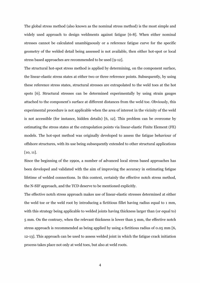
The effective notch stress approach makes use of linear-elastic stresses determined at either

the weld toe or the weld root by introducing a fictitious fillet having radius equal to 1 mm,

with this strategy being applicable to welded joints having thickness larger than (or equal to)

5 mm. On the contrary, when the relevant thickness is lower than 5 mm, the effective notch

stress approach is recommended as being applied by using a fictitious radius of 0.05 mm [6,

12-13]. This approach can be used to assess welded joint in which the fatigue crack initiation

process takes place not only at weld toes, but also at weld roots.

5

At the end of the 1990s, by taking full advantage of William’s analytical solution [14], Tovo

and Lazzarin formulated the so-called N-SIF approach [15, 16]. As far as failures at the weld

toes are concerned, the N-SIF approach estimates fatigue lifetime of welded components by

modelling the weld seams as V-notches having opening angle equal to 135° and root radius

equal zero [15-18]. The N-SIF approach can also be used to perform the fatigue assessment

of welded joints in which cracks initiate at the weld roots, provided that a specific reference

design curve is employed [16].

The TCD [19, 20] assesses the fatigue strength of welded joints by post-processing the

relevant linear-elastic local stress fields via a material characteristic length that is directly

related to the size of the dominant source of microstructural heterogeneity. According to the

TCD’s modus operandi, this critical distance is treated as a material property whose value is

independent from type of applied loading, geometry, notch profile, and size of the

component being assessed [5, 19-21].

In the complex scenario depicted above, the goal of the present investigation is to check the

accuracy of the aforementioned fatigue design methods in estimating fatigue lifetime of

aluminium welded joints against a large number of data taken from the literature. To use

both the hot-spot approach and the considered local stress methods to post-process the

experimental data being selected, a number of linear-elastic FE models was solved using

commercial FE code ANSYS®. The N-SIF approach was applied also by using the formulas

derived by Lazzarin and Tovo by post-processing the results from a large number of linear-

elastic FE models, with these formulas allowing the N-SIF range, ∆KI, to be estimated

directly for standard welded geometries [16, 17, 22, 23]. Finally, the N-SIF master curve

proposed by Lazzarin and Livieri [17, 21, 22] was used to determine a unifying value for the

TCD critical distance suitable for accurately estimating the fatigue lifetime of aluminium

welded joints.

6

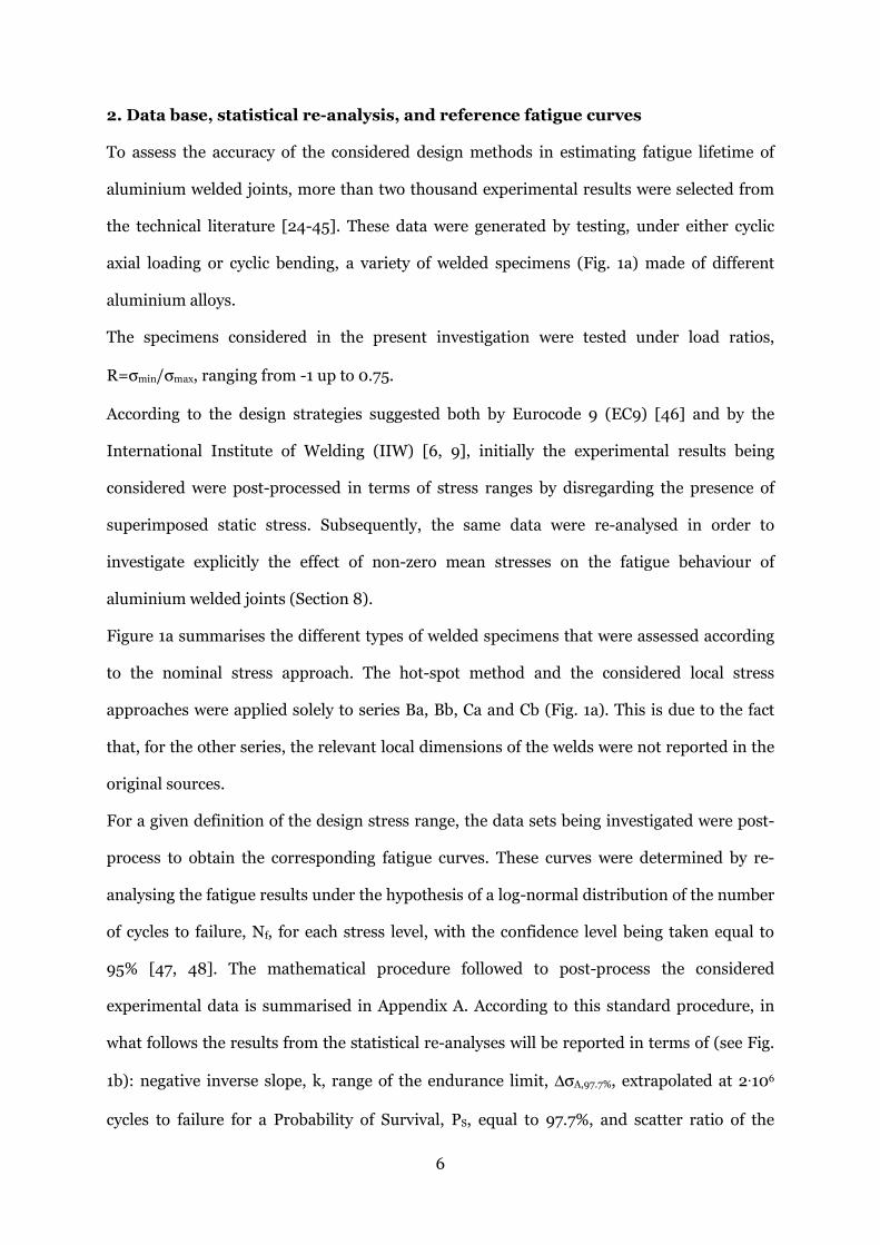
2. Data base, statistical re-analysis, and reference fatigue curves

To assess the accuracy of the considered design methods in estimating fatigue lifetime of

aluminium welded joints, more than two thousand experimental results were selected from

the technical literature [24-45]. These data were generated by testing, under either cyclic

axial loading or cyclic bending, a variety of welded specimens (Fig. 1a) made of different

aluminium alloys.

The specimens considered in the present investigation were tested under load ratios,

R=σmin/σmax, ranging from -1 up to 0.75.

According to the design strategies suggested both by Eurocode 9 (EC9) [46] and by the

International Institute of Welding (IIW) [6, 9], initially the experimental results being

considered were post-processed in terms of stress ranges by disregarding the presence of

superimposed static stress. Subsequently, the same data were re-analysed in order to

investigate explicitly the effect of non-zero mean stresses on the fatigue behaviour of

aluminium welded joints (Section 8).

Figure 1a summarises the different types of welded specimens that were assessed according

to the nominal stress approach. The hot-spot method and the considered local stress

approaches were applied solely to series Ba, Bb, Ca and Cb (Fig. 1a). This is due to the fact

that, for the other series, the relevant local dimensions of the welds were not reported in the

original sources.

For a given definition of the design stress range, the data sets being investigated were post-

process to obtain the corresponding fatigue curves. These curves were determined by re-

analysing the fatigue results under the hypothesis of a log-normal distribution of the number

of cycles to failure, Nf, for each stress level, with the confidence level being taken equal to

95% [47, 48]. The mathematical procedure followed to post-process the considered

experimental data is summarised in Appendix A. According to this standard procedure, in

what follows the results from the statistical re-analyses will be reported in terms of (see Fig.

1b): negative inverse slope, k, range of the endurance limit, ∆σA,97.7%, extrapolated at 2∙106

cycles to failure for a Probability of Survival, PS, equal to 97.7%, and scatter ratio of the

7

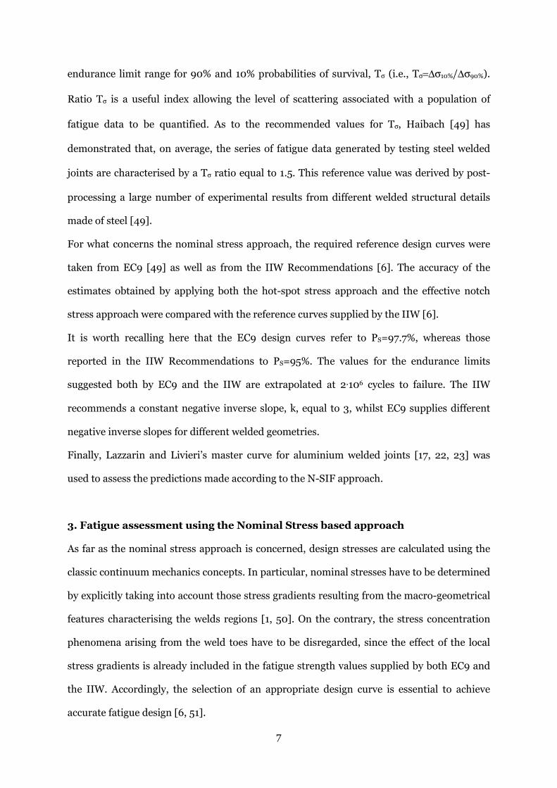
endurance limit range for 90% and 10% probabilities of survival, Tσ (i.e., Tσ=∆σ10%/∆σ90%).

Ratio Tσ is a useful index allowing the level of scattering associated with a population of

fatigue data to be quantified. As to the recommended values for Tσ, Haibach [49] has

demonstrated that, on average, the series of fatigue data generated by testing steel welded

joints are characterised by a Tσ ratio equal to 1.5. This reference value was derived by post-

processing a large number of experimental results from different welded structural details

made of steel [49].

For what concerns the nominal stress approach, the required reference design curves were

taken from EC9 [49] as well as from the IIW Recommendations [6]. The accuracy of the

estimates obtained by applying both the hot-spot stress approach and the effective notch

stress approach were compared with the reference curves supplied by the IIW [6].

It is worth recalling here that the EC9 design curves refer to PS=97.7%, whereas those

reported in the IIW Recommendations to PS=95%. The values for the endurance limits

suggested both by EC9 and the IIW are extrapolated at 2∙106 cycles to failure. The IIW

recommends a constant negative inverse slope, k, equal to 3, whilst EC9 supplies different

negative inverse slopes for different welded geometries.

Finally, Lazzarin and Livieri’s master curve for aluminium welded joints [17, 22, 23] was

used to assess the predictions made according to the N-SIF approach.

3. Fatigue assessment using the Nominal Stress based approach

As far as the nominal stress approach is concerned, design stresses are calculated using the

classic continuum mechanics concepts. In particular, nominal stresses have to be determined

by explicitly taking into account those stress gradients resulting from the macro-geometrical

features characterising the welds regions [1, 50]. On the contrary, the stress concentration

phenomena arising from the weld toes have to be disregarded, since the effect of the local

stress gradients is already included in the fatigue strength values supplied by both EC9 and

the IIW. Accordingly, the selection of an appropriate design curve is essential to achieve

accurate fatigue design [6, 51].

8

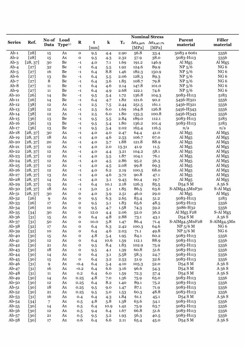
Tables 1 to 6 summarise the results obtained by using the nominal stress approach to post-

process, according to the statistical procedure reviewed in Appendix A, the individual data

sets being investigated. Endurance limit ranges ∆σA,50% and ∆σA,97.7% reported in Tables 1 to 6

were extrapolated at 2∙106 cycles to failure for PS equal to 50% and 97.7%, respectively.

These tables show that, on average, the negative inverse slope of the fatigue curves

determined from the individual series is larger than the values that are recommended both

by EC9 and by the IIW. Another important aspect is that, according to Tables 1 to 6, the

average value of Tσ is equal to 2.2 with a standard deviation of 1.3. This suggests that, as far

as aluminium welded joints are concerned, the expected value for Tσ is larger than the

reference value of 1.5 that is suggested by Haibach for steel weldments [49].

The experimental results listed in Tables 1 to 6 are also summarised in the Wöhler diagrams

reported in Figure 2. In more detail, these log-log charts plot the range of the nominal stress,

∆σnom, vs. the number of cycles to failure, Nf, for the different structural details being

considered (Fig. 1a). For each welded geometry, the fatigue curves suggested by EC9 (grey

continuous line) and the IIW (black continuous line) are also plotted in Figure 2 to allow the

experimental results to be contrasted with the standard/recommended design guidelines.

The fatigue curves for PS=50% and PS=97.7% determined, according to the statistical

procedure reviewed in Appendix A, by post-processing all the experimental results generated

by testing the same type of structural detail are summarised in Table 7. In this table, the

obtained values are directly compared to the corresponding design curves in terms of

negative inverse slope and endurance limit range extrapolated at 2∙106 cycles to failure.

Figure 2 shows that, in general, the design curves recommended by EC9 result in more

conservative estimates than those obtained by using the IIW design curves. Further, these

Wöhler diagrams together with Table 7 demonstrate that, for a given welded geometry, the

negative inverse slope calculated from the entire population of data is lower than the

corresponding value suggested by both EC9 and the IIW. This is an interesting aspect,

especially in light of the fact that, as shown in Tables 1 to 6, the negative inverse slope of the

individual data sets is, in general, larger than the corresponding standard value.

9

Finally, it is important to highlight that the use of the design curves recommended both by

EC9 and by the IIW to assess butt (Ab) and load-carrying cruciform (Ca) welded joints is

seen to result in estimates that are slightly non-conservative.

4. Fatigue assessment using the Hot-Spot Stress approach

The Hot-Spot Stress approach takes as its starting point the idea that the gradient

characterising the stress field distribution in the vicinity of the weld toe can be modelled

effectively via the linear-elastic stress states determined at two or three reference superficial

points positioned at given distances from the weld toe itself [52]. Subsequently, via these

reference stress states, structural stresses are extrapolated to the weld toes at the hot spots

(Fig. 3a). By so doing, the effects of the local stress gradients can be taken into account

indirectly via specific reference fatigue curves [6, 53].

In situations of practical interest, the Hot-Spot Stress approach is applied by determining

the required reference stresses using strain gauges and/or solving linear-elastic FE models.

In the latter case, hot-spot stresses can be estimated either via surface stress extrapolation or

via through thickness stress linearization [6, 53]. Another interesting method is the one

proposed by Dong which is based on the linearized equilibrium of the normal and shear

stresses acting on the weld toe region where the effect of the local stress singularities can be

neglected with little loss of accuracy [54].

In the present investigation, hot-spot stresses were determined numerically according to the

IIW procedure which is based on the use of different reference distances, with these lengths

depending on type of hot-spot stress and quality of mesh [6]. Linear-elastic bi-dimensional

FE models were solved via commercial software ANSYS®. Weld beads were modelled as

sharp V-notches, i.e., by taking the fillet radius along the intersection line between weld and

parent material invariably equal to zero. The models were meshed according to the rules

recommended by the IIW via eight-noded solid quadratic elements (Plane 183). The mesh

density was varied throughout the welded details in order to obtain in the vicinity of the weld

toes finely meshed regions with element size in the range 0.2-0.3 mm (Fig. 4a). Parent and

10

filler aluminium alloys were treated as linear-elastic, isotropic and homogenous materials

with Young’s modulus equal to 68 GPa and Poisson’s ratio equal to 0.33 [19]. Via these FE

models, the corresponding hot-spot stresses were calculated using the surface stress

extrapolation method as shown in Figure 3a. In particular, normal stresses were determined

at two reference points positioned at a distance from the weld toe equal to 0.4∙t and t,

respectively, with t being the thickness of the main plate as defined in Figure 1a [6].

The results from the statistical re-analysis performed by post-processing structural welded

details Ba, Bb, Ca and Cb (Fig. 1a) according to the Hot-Spot Stress approach are

summarised in Tables 8 to 11. The same data are also plotted in the Wöhler diagrams

reported in Figure 3b. The values of both the negative inverse slope, k, and the endurance

limit range (∆σA,50% and ∆σA,97.7%) at 2∙106 cycles to failure that were determined by re-

analysing, for any given welded geometry, the entire population of data are reported in Table

7.

The Wöhler diagrams of Figure 3b demonstrate that, as long as non-load-carrying cruciform

connections (Ba) and T-joints (Bb) are concerned, the use of the hot-spot approach together

with the design fatigue curves supplied by the IIW resulted in estimates that are not only

accurate, but also characterised by an adequate level of conservatism. On the contrary, the

use of the IIW design curves returned estimates that are characterised by a certain degree of

non-conservatism when they are employed to assess the strength of load-carrying fillet

welded joints (series Ca and Cb in Figure 1a). As to this aspect, it is interesting to observe

that for these welded geometries the level of non-conservatism is seen to increase as the load

ratio increases.

To conclude, according to both Figure 3b and Table 7, it can be noted that, for a given type of

structural detail, the negative inverse slopes determined by reanalysing the entire population

of data are lower not only than the k values associated with the individual data sets (Tables 8

to 11), but also than the unifying value of 3 recommended by the IIW.

11

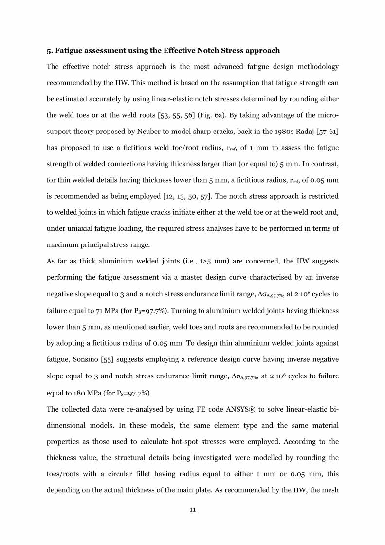
5. Fatigue assessment using the Effective Notch Stress approach

The effective notch stress approach is the most advanced fatigue design methodology

recommended by the IIW. This method is based on the assumption that fatigue strength can

be estimated accurately by using linear-elastic notch stresses determined by rounding either

the weld toes or at the weld roots [53, 55, 56] (Fig. 6a). By taking advantage of the micro-

support theory proposed by Neuber to model sharp cracks, back in the 1980s Radaj [57-61]

has proposed to use a fictitious weld toe/root radius, rref, of 1 mm to assess the fatigue

strength of welded connections having thickness larger than (or equal to) 5 mm. In contrast,

for thin welded details having thickness lower than 5 mm, a fictitious radius, rref, of 0.05 mm

is recommended as being employed [12, 13, 50, 57]. The notch stress approach is restricted

to welded joints in which fatigue cracks initiate either at the weld toe or at the weld root and,

under uniaxial fatigue loading, the required stress analyses have to be performed in terms of

maximum principal stress range.

As far as thick aluminium welded joints (i.e., t≥5 mm) are concerned, the IIW suggests

performing the fatigue assessment via a master design curve characterised by an inverse

negative slope equal to 3 and a notch stress endurance limit range, ∆σA,97.7%, at 2∙106 cycles to

failure equal to 71 MPa (for PS=97.7%). Turning to aluminium welded joints having thickness

lower than 5 mm, as mentioned earlier, weld toes and roots are recommended to be rounded

by adopting a fictitious radius of 0.05 mm. To design thin aluminium welded joints against

fatigue, Sonsino [55] suggests employing a reference design curve having inverse negative

slope equal to 3 and notch stress endurance limit range, ∆σA,97.7%, at 2∙106 cycles to failure

equal to 180 MPa (for PS=97.7%).

The collected data were re-analysed by using FE code ANSYS® to solve linear-elastic bi-

dimensional models. In these models, the same element type and the same material

properties as those used to calculate hot-spot stresses were employed. According to the

thickness value, the structural details being investigated were modelled by rounding the

toes/roots with a circular fillet having radius equal to either 1 mm or 0.05 mm, this

depending on the actual thickness of the main plate. As recommended by the IIW, the mesh

12

in the vicinity of the fictitious fillets was refined until convergence occurred (Fig 4b). This

refinement process led to elements having size in the critical regions ranging between 0.04-

0.06 mm for rref=1 mm and between 0.0025-0.0035 mm for rref=0.05 mm.

The results from the statistical re-analysis performed by post-processing welded geometries

Ba, Bb, Ca and Cb (Fig. 1a) in terms of linear-elastic notch stress are listed in Tables 8 to 11.

The individual experimental results are plotted instead in the log-log charts of Figure 5b.

Table 7 lists the values of k as well as of ∆σA,50% and ∆σA,97.7% at 2∙106 cycles to failure

determined by re-analysing the entire population of data for any welded geometry being

considered.

The Wöhler diagrams of Figure 5b show that the use of the Effective Notch Stress approach

along with the design fatigue curve supplied by the IIW [6] for t≥5 mm and by Sonsino [55]

for t<5 mm resulted in estimates that are not only accurate, but also characterised by an

adequate level of conservatism.

To conclude, according to both Figure 5b and Table 7, although the in-field usage of this

approach requires a considerable computational effort, the Effective Notch Stress approach

certainly is the most accurate design method amongst those recommended by the IIW.

6. Fatigue assessment using N-SIF approach

According to Williams [14], linear-elastic stress fields in the vicinity of V-notches with root

radius, rn, equal to zero can be written as follows for Mode I and Mode II loading,

respectively [15] (Fig. 6a):

θλ+

θλ+−

θλ+

λ−χ+

θλ−λ−

θλ−λ−

θλ−λ+

⋅λ−χ+λ+π

=

τ

σ

σ−λ

=θ

θ

)1sin(

)1cos(

)1cos(

)1(

)1sin()1(

)1cos()3(

)1cos()1(

)1()1(

Kr

2

1

1

1

1

11

11

11

11

111

I1

0rr

r

1

n

(1)

θλ+

θλ+

θλ+−

λ+χ+

θλ−λ−

θλ−λ−−

θλ−λ+−

⋅λ+χ+λ−π

=

τ

σ

σ−λ

=θ

θ

)1cos(

)1sin(

)1sin(

)1(

)1cos()1(

)1sin()3(

)1sin()1(

)1()1(

Kr

2

1

2

2

2

22

22

22

22

222

II1

0rr

r

2

n

(2)

13

where λi and χi (i=1, 2) are parameters that depend on the opening angle of the V-notch

being assessed [15, 62]. KI and KII are the N-SIFs for Mode I and Mode II loading,

respectively, and are defined as follows:

( )[ ]11

00r

I rlim2K λ−

=θθ→

σπ= (3)

( )[ ]21

0r0r

II rlim2K λ−

=θθ→

τπ= (4)

The N-SIF approach was first proposed by Verreman and Nie [63] back in the mid-1990s.

This approach takes as a starting point the fact that [64, 65], according to Eqs (1) and (2),

linear-elastic stress fields in the vicinity of sharp V-notches can be described concisely by

using N-SIFs. Accordingly, Verreman and Nie argued that this stress parameters could be

employed directly to model the crack-initiation process in fillet welded joints subjected to

fatigue loading [63]. A couple of years later, this approach was further developed by Tovo

and Lazzarin who devised a more rigorous theoretical framework by proposing a formal

definition for the N-SIFs [15]. In particular, they observed that in fillet welded joints under

nominal axial loading the contribution due to the Mode II stress components can be

neglected with little loss of accuracy. This is a consequence of the fact that Mode II stresses

are no longer singular for opening angles larger than about 100° [15, 62]. The accuracy and

reliability of the N-SIF approach was initially checked by considering steel fillet welded joints

with thickness varying in the range 13-100 mm. Subsequently, Lazzarin and Livieri extended

the use of this design method to aluminium welded joints by proposing a specific design

curve that was derived by considering a large number of experimental data [22]. This master

curve is characterised by a reference Mode I N-SIF range, ∆KI,97.7%, at 5∙106 cycles to failure

equal to 74 MPa∙mm0.326 (for PS=97.7%) and a negative inverse slope equal to 4.

14

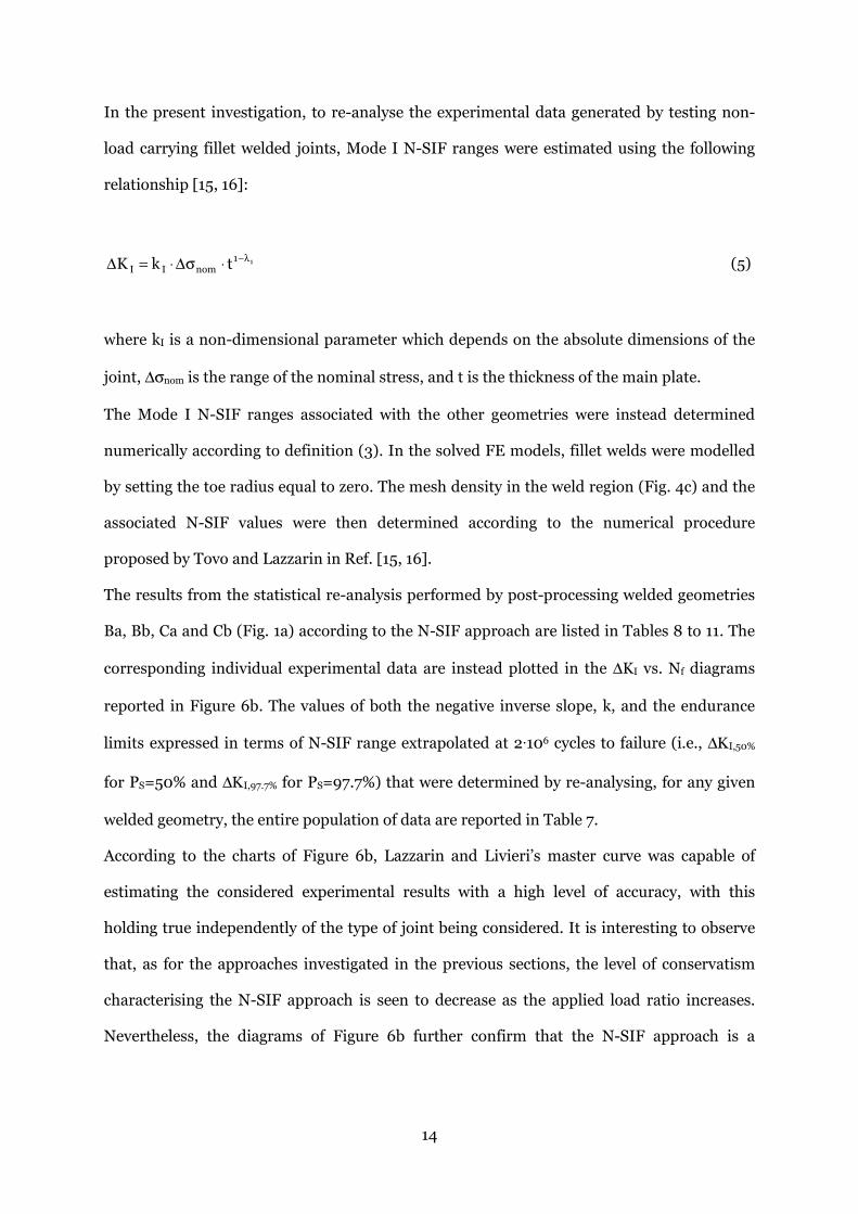
In the present investigation, to re-analyse the experimental data generated by testing non-

load carrying fillet welded joints, Mode I N-SIF ranges were estimated using the following

relationship [15, 16]:

11nomII tkK λ−⋅σ∆⋅=∆ (5)

where kI is a non-dimensional parameter which depends on the absolute dimensions of the

joint, ∆σnom is the range of the nominal stress, and t is the thickness of the main plate.

The Mode I N-SIF ranges associated with the other geometries were instead determined

numerically according to definition (3). In the solved FE models, fillet welds were modelled

by setting the toe radius equal to zero. The mesh density in the weld region (Fig. 4c) and the

associated N-SIF values were then determined according to the numerical procedure

proposed by Tovo and Lazzarin in Ref. [15, 16].

The results from the statistical re-analysis performed by post-processing welded geometries

Ba, Bb, Ca and Cb (Fig. 1a) according to the N-SIF approach are listed in Tables 8 to 11. The

corresponding individual experimental data are instead plotted in the ∆KI vs. Nf diagrams

reported in Figure 6b. The values of both the negative inverse slope, k, and the endurance

limits expressed in terms of N-SIF range extrapolated at 2∙106 cycles to failure (i.e., ∆ΚI,50%

for PS=50% and ∆ΚI,97.7% for PS=97.7%) that were determined by re-analysing, for any given

welded geometry, the entire population of data are reported in Table 7.

According to the charts of Figure 6b, Lazzarin and Livieri’s master curve was capable of

estimating the considered experimental results with a high level of accuracy, with this

holding true independently of the type of joint being considered. It is interesting to observe

that, as for the approaches investigated in the previous sections, the level of conservatism

characterising the N-SIF approach is seen to decrease as the applied load ratio increases.

Nevertheless, the diagrams of Figure 6b further confirm that the N-SIF approach is a

15

powerful design tool suitable for designing aluminium welded joint against fatigue by

systematically reaching an adequate level of accuracy/safety.

7. Fatigue assessment using the TCD

As far as notched components are concerned, the TCD assesses the detrimental effect of

stress gradients by post-processing the entire linear-elastic stress fields acting on the

material in the vicinity of the assumed crack initiation locations [19, 20]. The key feature of

this theory is that the required design stress is determined via a specific length scale

parameter that takes into account the microstructural features of the material being

assessed. The TCD can be formalised in different ways that include the Point Method (PM),

Line Method (LM), Area Method (AM), and Volume Method (VM) [5, 20]. The PM and the

LM were first introduced in about the mid of the last century by Peterson [66] and Neuber

[67], respectively, to perform the high-cycle fatigue assessment of notched metallic

materials. In these formalisations of the TCD, the required critical distances were

determined empirically by post-processing a large number of experimental results.

Subsequently, in the 1980s-1990s Tanaka [68] and Taylor [19] provided a simple way to

estimate the critical distance value, with this well-known formula being based on the

combined use of the Linear Elastic Fracture Mechanics mechanical properties and the plain

material fatigue strength.

The PM represents the simplest formalisation of the TCD and postulates that the stress to be

used to estimate the fatigue damage extent is equal to the linear elastic-stress determined at

a given distance from the assumed crack initiation location. Its simplicity makes the PM a

straightforward design tool suitable for being used in situations of practical interest to

perform the fatigue assessment of real welded components. Accordingly, in the present

investigation the accuracy of the TCD in estimating fatigue lifetime of aluminium welded

joints was checked by applying this powerful theory solely in the form of the PM.

Following a strategy similar to the one adopted in Ref. [5], the PM was calibrated by making

the following assumptions:

16

• the fatigue strength of ground butt welded joints under uniaxial fatigue loading is

modelled via the EC9 fatigue curve recalculated for PS=50% (i.e., ∆σA,50%=79.2MPa at

2∙106 cycles to failure and k=4.5);

• the PS=50% reference master curve suggested by Lazzarin and Livieri for aluminium

welded joints (∆KI,50%=124.5 MPa∙mm0.326 at 2∙106 cycles to failure and k=4 [22]) is

used as reference notch fatigue curve.

By using these two pieces of calibration information, a unifying value for the critical distance,

LW-Al, suitable for designing aluminium welded joints was then determined as follows:

• by making t, L and z vary (see welded geometry Ca in Figure 1a), the PS=50% N-SIF

master curve and Eq. (5) were used to estimate the corresponding nominal stress

range, ∆σnom,50%, at 2∙106 cycles to failure;

• subsequently, under the estimated values for ∆σnom,50%, the corresponding local stress

distributions were determined along the weld toe bisector in terms of maximum

principal stress ∆σ1 (Fig. 6a) [4, 5], with these stress-distance curves being estimated

both numerically (Fig. 4c) and analytically via Eq. (1);

• finally, according to the PM, by plotting, at 2∙106 cycles to failure, the linear-elastic

stress field for the welded geometry being considered as well as the ground butt weld

endurance limit, i.e.. ∆σA,50%=79.2 MPa, critical distance value LW-Al was estimated

directly via the abscissa of the point at which these two stress-distance curves crossed

each other (Fig. 6a).

Since Lazzarin and Livieri’s N-SIF master curve was determined by post-processing a large

number of experimental data generated by testing aluminium cruciform joints having

absolute dimensions in the range 3-24mm [22, 23], the procedure describe above was

17

applied by considering different values for t, L and z (see welded geometry Ca in Figure 1a).

This was done in order to check whether the estimated critical distances were affected by the

absolute dimensions of the welded joint being used for calibration (scale effect in fatigue).

Table 12 summarises the results of this sensitivity analysis that was performed by taking t, L

and z equal to 8, 12, 16 and 20mm. Table 12 demonstrates that, from an engineering point of

view, the influence of the welded connection’s absolute dimensions on the estimated values

for length LW-Al can be neglected with little loss of accuracy. Accordingly, for the sake of

design simplicity, the LW-Al/2 value to apply the PM to design aluminium welded joints

against fatigue was taken invariably equal to 0.25 mm, i.e.:

LW-Al = 0.5 mm (6)

Once the critical distance was determined, the experimental results summarised in Tables 8

to 11 were post-processed to determine the linear-elastic PM stress range, ∆σPM, at a distance

from the weld toe equal to LW-Al/2=0.25 mm (Fig. 6a), the required linear-elastic stress fields

being determined by taking the weld toe radius invariably equal to zero. The experimental

results summarised in the above tables are also plotted in the ∆σPM vs. Nf log-log diagrams

reported in Figure 6b, the PS=97.7% reference design curve being that recommended by EC9

to assess the fatigue strength of ground butt welded joints (i.e., ∆σA,97.7%=55 MPa at 2∙106

cycles to failure and k=4.5). These charts make it evident that the TCD applied by taking

LW-Al/2=0.25 mm resulted in highly accurate estimates, with this holding true independently

of type of joint and absolute dimensions. It is also interesting to observe that, according to

Table 7, the negative inverse slope, k, determined, for any considered welded geometry, by

post-processing the entire population of data was seen to be lower than the value of 4.5

characterising the EC9 design curve used as reference information not only to estimate LW-Al,

but also to assess the overall accuracy of the PM (Fig. 6b). This results in the fact that, as for

the other design methods being considered in the present investigation, the endurance limits

18

for series Ba, Bb, Ca and Cb were seen to be lower than the corresponding endurance limit of

the EC9 reference design fatigue curve being adopted (see Table 7).

To conclude, the charts of Figure 6b fully support the idea that the TCD can be used to

perform the fatigue assessment of aluminium weldments by directly post-processing the

linear-elastic stress fields acting on the material in the weld regions. Its systematic usage was

seen to result in highly accurate estimates, the computational effort required for its in-field

usage being lower than the one required to apply both the Effective Notch Stress method and

the N-SIF approach.

8. Effect of non-zero mean stresses on the fatigue strength of aluminium

weldments

Independent of the definition being adopted to determine the required design stress, much

experimental evidence suggests that, as far as-welded connections are concerned, the

presence of superimposed static stresses plays a minor role in the overall fatigue strength of

welded joints [53]. This is a consequence of the fact that the residual stresses arising from

the welding process alter the actual value of the load ratio in the vicinity of the crack

initiation locations. Therefore, in the presence of high tensile residual stresses, the local

value of R is seen to be different from the nominal load ratio characterising the load history

under investigation, with the local R ratio becoming larger than zero also under fully-

reversed nominal fatigue loading. Accordingly, connections in the as-welded condition are

usually assessed via reference design curves that are determined experimentally under R>0.

Whilst the above simplification is seen to result in reasonable fatigue life predictions for steel

welded joints, unfortunately, it does not always return satisfactory results with aluminium

weldments. This is due to the fact that nominal load ratios lower than zero can affect the

fatigue behaviour not only of stress relieved, but also of as-welded aluminium joints [12].

Accordingly, under nominal load rations lower than zero, fatigue assessment performed by

following the recommendations of the available standard can lead to an excessive level of

conservatism. The effect of residual stresses can be mitigated by relieving the material in the

19

weld regions via appropriate technological processes. However, by so doing, aluminium

weldments’ fatigue strength is seen to increase, with the role played by non-zero mean

stresses becoming more and more important as load ratio R decreases [53].

Both EC9 and the IIW suggest to use specific enhancement factors in order to take into

account the effect of the load ratio characterising the load history being assessed.

Enhancement factor f(R) is defined as the ratio between the actual value of the endurance

limit at 2∙106 cycles to failure and the corresponding design endurance limit recommended

as being used for the specific welded geometry being designed. In other words, from a fatigue

assessment point of view, under R<0.5 the fatigue strength of the specific welded detail

being designed can be increased by multiplying the corresponding fatigue class by f(R).

Both EC9 [46] and the IIW [6] considers the following three scenarios:

• Case I. Un-welded base material and wrought products with negligible residual

stresses; stress relieved welded components, in which the effects of constraints or

secondary stresses have been considered in analysis; no constraints in assembly:

6.1)R(f = for R<-1

2.1R4.0)R(f +⋅−= for -1≤R≤0.5 (7)

1)R(f = for R>0.5

• Case II. Small scale thin-walled simple structural elements containing short welds;

parts or components containing thermally cut edges; no constraints in assembly:

3.1)R(f = for R<-1

9.0R4.0)R(f +⋅−= for -1≤R≤-0.25 (8)

1)R(f = for R>-0.25

20

• Case III. Complex two- or three-dimensional welded components; components with

global residual stresses; thick-walled components; normal case for welded components

and structures:

1)R(f = (9)

In order to check the accuracy and reliability of the enhancement factors reported above for

Case I and Case II, all the data considered in the present investigation were post-processed

to compare the experimental value of f(R) to the corresponding value estimated according to

rules (7) and (8). In particular, independently of type of welded joint and adopted definition

for the design stress, the experimental values for the enhancement factors were calculated as

follows:

classfatigue%7.97,A

erimentalexp%7.97,A

)R(fσ∆

σ∆= or

classfatigue%95,A

erimentalexp%95,A

)R(fσ∆

σ∆= (10)

In a similar way, the enhancement factors for the N-SIF approach were determined as:

curvemaster%7.97,I

erimentalexp%7.97,I

K

K)R(f

∆

∆= (11)

The results of this analysis are summarised in the f(R) vs. R diagrams of Figures 8a to 8f.

These charts make it evident that, independently of the adopted design strategy, the

experimentally determined values for enhancement factor f(R) are highly scattered.

However, in spite of such a large level of scattering, the diagrams of Figures 8a to 8f confirm

that, on average, the fatigue strength of aluminium welded joints tends to increase as the

load ratio decreases.

21

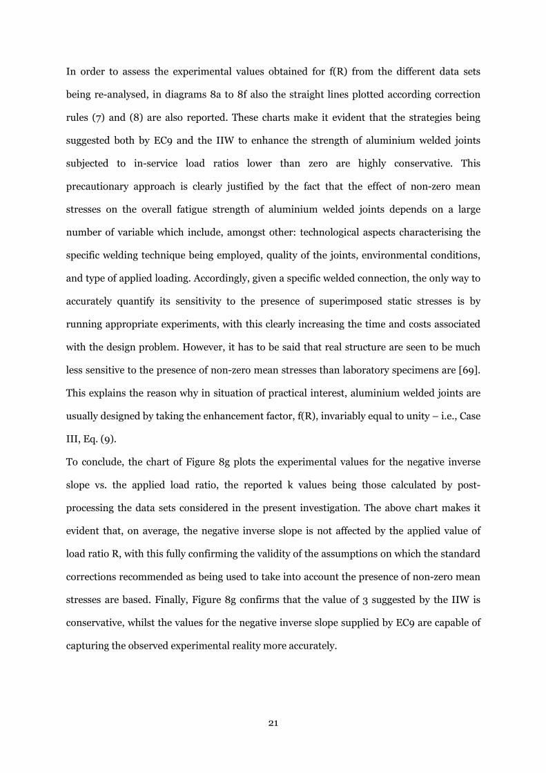
In order to assess the experimental values obtained for f(R) from the different data sets

being re-analysed, in diagrams 8a to 8f also the straight lines plotted according correction

rules (7) and (8) are also reported. These charts make it evident that the strategies being

suggested both by EC9 and the IIW to enhance the strength of aluminium welded joints

subjected to in-service load ratios lower than zero are highly conservative. This

precautionary approach is clearly justified by the fact that the effect of non-zero mean

stresses on the overall fatigue strength of aluminium welded joints depends on a large

number of variable which include, amongst other: technological aspects characterising the

specific welding technique being employed, quality of the joints, environmental conditions,

and type of applied loading. Accordingly, given a specific welded connection, the only way to

accurately quantify its sensitivity to the presence of superimposed static stresses is by

running appropriate experiments, with this clearly increasing the time and costs associated

with the design problem. However, it has to be said that real structure are seen to be much

less sensitive to the presence of non-zero mean stresses than laboratory specimens are [69].

This explains the reason why in situation of practical interest, aluminium welded joints are

usually designed by taking the enhancement factor, f(R), invariably equal to unity – i.e., Case

III, Eq. (9).

To conclude, the chart of Figure 8g plots the experimental values for the negative inverse

slope vs. the applied load ratio, the reported k values being those calculated by post-

processing the data sets considered in the present investigation. The above chart makes it

evident that, on average, the negative inverse slope is not affected by the applied value of

load ratio R, with this fully confirming the validity of the assumptions on which the standard

corrections recommended as being used to take into account the presence of non-zero mean

stresses are based. Finally, Figure 8g confirms that the value of 3 suggested by the IIW is

conservative, whilst the values for the negative inverse slope supplied by EC9 are capable of

capturing the observed experimental reality more accurately.

22

9. Conclusions

• The use of the design curves recommended both by EC9 and the IIW to perform the

fatigue assessment of aluminium welded joints according to the Nominal Stress

approach is seen to result in an adequate level of accuracy, with the estimates being,

on average, conservative.

• The data sets considered in the present investigation fully confirm the fact that the

Hot-Spot approach can be used successfully to design real aluminium welded joints

against fatigue.

• The Effective Notch Stress approach is seen to be the most accurate design

methodology recommended by the IIW. However, it requires intensive computational

effort to model weld toes and roots by introducing the required fillet radii (with this

holding true especially in the presence of complex three-dimensional welded

geometries).

• The re-analysis discussed in the present paper further confirms the notorious

accuracy of the N-SIF approach in estimating fatigue lifetime of aluminium welded

joints.

• The TCD applied in the form of the PM is seen to be highly accurate in assessing the

strength of aluminium welded joints subjected to fatigue loading.

• The TCD can be used in situations of practical interest to design, in terms of

maximum principal stress, aluminium welded joints against fatigue by taking the

required critical distance value, LW-Al, invariably equal to 0.5 mm.

• As far as aluminium welded joints are concerned, the enhancement factors

recommended both by EC9 and the IIW are seen to result in conservative estimates.

Accordingly, experimental trials should be run in order to assess accurately the

sensitivity of the specific welded joints being designed to the presence of non-zero

mean stresses.

23

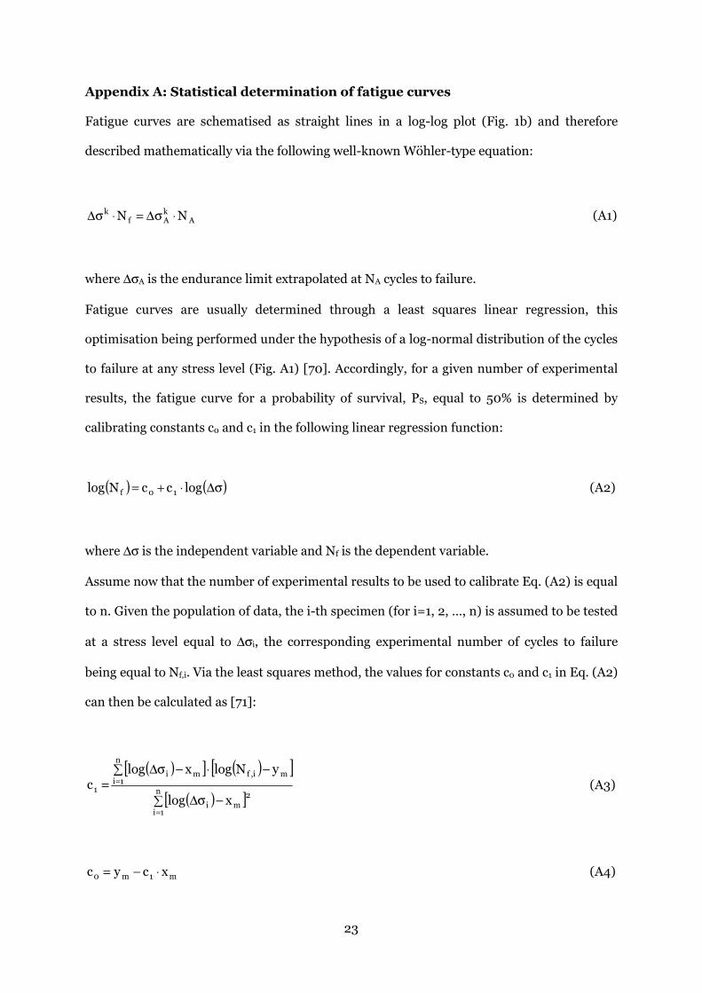
Appendix A: Statistical determination of fatigue curves

Fatigue curves are schematised as straight lines in a log-log plot (Fig. 1b) and therefore

described mathematically via the following well-known Wöhler-type equation:

AkAf

k NN ⋅σ∆=⋅σ∆ (A1)

where ∆σA is the endurance limit extrapolated at NA cycles to failure.

Fatigue curves are usually determined through a least squares linear regression, this

optimisation being performed under the hypothesis of a log-normal distribution of the cycles

to failure at any stress level (Fig. A1) [70]. Accordingly, for a given number of experimental

results, the fatigue curve for a probability of survival, PS, equal to 50% is determined by

calibrating constants c0 and c1 in the following linear regression function:

( ) ( )σ∆⋅+= logccNlog 10f (A2)

where ∆σ is the independent variable and Nf is the dependent variable.

Assume now that the number of experimental results to be used to calibrate Eq. (A2) is equal

to n. Given the population of data, the i-th specimen (for i=1, 2, …, n) is assumed to be tested

at a stress level equal to ∆σi, the corresponding experimental number of cycles to failure

being equal to Nf,i. Via the least squares method, the values for constants c0 and c1 in Eq. (A2)

can then be calculated as [71]:

( )[ ] ( )[ ]

( )[ ]∑ −σ∆

∑ −⋅−σ∆=

=

=

n

1i

2mi

n

1imi,fmi

1

xlog

yNlogxlogc (A3)

m1m0 xcyc ⋅−= (A4)

24

where

( )

n

logx

n

ii

m

∑ σ∆= (A5)

( )

n

Nlogy

n

ii,f

m

∑= (A6)

As soon as constants c0 and c1 are known, both the negative inverse slope, k, and the

endurance limit, ∆σA,50%, extrapolated for PS=50% at NA cycles to failure can directly be

determined by simply rewriting Eq. (A1) in the form of Eq. (A2), obtaining:

1ck −= (A7)

k

1

A

c

%50,AN

10 0

=σ∆ (A8)

To determine the scatter band characterising the population of experimental data being post-

process, initially the associated standard deviation has to be calculated according to the

following standard formula:

( )

1n

NlogNlog

s

n

1i

2k

i

%50,AAi,f

−

∑

σ∆

σ∆−

==

(A9)

25

Standard deviation s allows the endurance limit at NA cycles to failure to be estimated

directly for PS=P% and PS=(1-P)%, respectively (Fig. A1), i.e.:

( )

k/1

sqNlogA

%50,A%P,AA10

N

σ∆=σ∆

⋅+ (A10)

( )

k/1

sqNlogA

%50,A)%P1(,AA10

N

σ∆=σ∆

⋅−− , (A11)

In Eqs (A10) and (A11) q is a statistical index that depends on the adopted confidence level,

the chosen probability of survival, and the number of tested samples [48]. Table A1 lists, for

different probabilities of survival, some values of index q determined, under the hypothesis

of a log-normal distribution, by taking the confidence level equal to 95% [72].

To conclude, it is worth highlighting that the curves determined for PS equal to P% and to

(1-P)% have both negative inverse slope, k, equal to that of the Wöhler curve determined for

PS=50% - Eq. (A8).

References

[1] Fricke W. Review Fatigue analysis of welded joints: state of development. Mar Struc

2003;16(3):185-200.

[2] Borrego LP, Costa JD, Jesus JS, Loureiro AR, Ferreira, JM. Fatigue life improvement by

friction stir processing of 5083 aluminium alloy MIG butt welds. Theor Appl Fract Mec

2014;70:68-74.

[3] Haryadi GD, Kim SJ. Influences of post weld heat treatment on fatigue crack growth

behavior of TIG welding of 6013 T4 aluminium alloy joint (part 1. Fatigue crack growth

across the weld metal). J Mech Sci Technol 2011;25(9):2161-2170.

[4] Susmel L. Multiaxial notch fatigue: from nominal to local stress/strain quantities.

Woodhead Publishing Limited, Cambridge, UK 2009.

[5] Susmel L. The Mdified Wöhler Curve Method calibrated by using standard fatigue curves

and applied in conjunction with the Theory of Critical Distances to estimate fatigue lifetime

of aluminium weldments. Int J Fatigue 2009;31:197-212.

26

[6] Hobbacher A. Recommendations For Fatigue Design of Welded Joints and Components

IIW document XIII-2151-07/XV-1254-07, 2007.

[7] Susmel L. Four Stress analysis strategies to use the Modified Wöhler Curve Method to

perform the fatigue assessment of weldments subjected to constant and variable amplitude

multiaxial fatigue loading. Int J Fatigue 2014;67:38-54.

[8] Aygul M. Fatigue Analysis of Welded Structures Using the Finite Element Method. Ph.D

thesis, Chalmers University of Technology, Gothenburg, Sweden, 2012 (available at:

http://publications.lib.chalmers.se/records/fulltext/155710.pdf)

[9] Hobbacher AF. New developments at the recent update of the IIW recommendations for

fatigue of welded joints and components. Steel Construction 2010;3(4):231-242.

[10] Niemi E, Fricke W, Maddox SJ. Fatigue Analysis of Welded Components: Designer's

Guide to the Structural hot spot stress approach (IIW-1430-00). Woodhead Publishing

Limited, Cambridge, UK, 2006.

[11] Niemi E. Structural stress approach to fatigue analysis of welded components. IIW-

document XIII-1819-00/XV-1090-01, 2000.

[12] Morgenstern C, Sonsino CM, Hobbacher A, Sorbo F. Fatigue design of aluminium

welded joints by the local stress concept with the fictitious notch radius of rf=1mm. Int J

Fatigue 2006;28:881-890.

[13] Karakas O, Morgenstern C, Sonsino CM. Fatigue design of welded joints from the

wrought magnesium alloy AZ31 by the local stress concept with the fictitious notch radii of

rf=1.0 and 0.05mm. Int J Fatigue 2008;30:2210-2219.

[14] Williams ML. Stress singularities resulting from various boundary conditions in angular

corners of plates in extension. J Appl Mech 1952;19:526–8.

[15] Lazzarin P, Tovo R. A unified approach to the evaluation of linear elastic stress fields in

the neighborhood of cracks and notches. Int J Fracture 1996;78:3-19.

[16] Lazzarin P, Tovo R. A notch intensity factor approach to the stress analysis of welds.

Fatigue Fract Engng Mater Struct 1998;21:1089-1103.

[17] Lazzarin P, Lassen T, Livieri P. A notch stress intensity approach applied to fatigue life

predictions of welded joints with different local toe geometry. Fatigue Fract Engng Mater

Struct, 2003;26:49-58.

[18] Atzori B, Lazzarin P, Meneghetti G. Fatigue Strength Assessments of Welded Joints:

from the Integration of Paris' Law to Synthesis Based on the Notch Stress Intensity Factors

of the Uncracked Geometries. Eng Fract Mech 2008;75(3-4):364-378.

[19] Taylor D, Barrett N, Lucano G. Some new methods for predicting fatigue in welded

joints. Int J Fatigue 2002;24:509-518.

[20] Crupi G, Crupi V, Guglielmino E, Taylor D. Fatigue assessment of welded joints using

critical distance and other methods. Eng Fail Anal 2005;12:129-142.

27

[21] Susmel L, Taylor D. A novel formulation of the theory of critical distances to estimate

lifetime of notched components in the medium-cycle fatigue regime. Fatigue Fract Engng

Mater Struct 2007;30:567-581.

[22] Livieri P, Lazzarin P. Fatigue strength of steel and aluminium welded joints based on

generalised stress intensity factors and local strain energy values. Int J Fracture

2005:133(3):247–276.

[23] Lazzarin P, Livieri P. Notch stress intensity factors and fatigue strength of aluminium

and steel welded joints. Int J Fatigue 2001;23:225-232.

[24] Neumann A. Theortische Grundlagen der Austwertung von Dauerfestigkeistversuchen

aus Schweibverbindungen und geschweibten Bauteilen aus Al Mg- Legierungen

Wissenschaftl. Wissenschaftliche Zeitschrift der Technischen Universität Karl-Marx-Stadt,

Chemnitz, Germany, 1965.

[25] Anon. Minutes of the meeting of the Working Group on fatigue issues in shipbuilding.

The Shipbuilding Engineering Society, Blohm & Voss AG, Hamburg, 1973

(www.blohmvoss.com).

[26] Person NL, Fatigue of aluminium alloy welded joints. Welding Research Supplement

1971:3;77s-87s.

[27] Wood JL. Flexural fatigue strength of butt welds in Np.5/6 type aluminium alloy. British

Welding Journal 1970;7(5):365-380.

[28] Atzori B, Bufano R. Raccolta di dati sulla resistenza a fatica dei giunti saldati in Al Mg5.

University of Bari, Bari, Italy, Report no. 76/4, November 1976

[29] Haibach E, Kobler HG. Beurteilung der Schwingfestigkeit von Schweibverbindungen

aus AlZnMgi auf dem Weg einer ortlichen Dehnungsmessung. Aluminium 1971;47:725-730.

[30] Mindlin H. Fatigue of Aluminium Magnesium Alloys. Welding Research Supplement

1963;1:276-281.

[31] Gunn KW, McLester R. Effect of Mean Stress on Fatigue Properties of Aluminum Butt-

Welded Joints. Welding Research Abroad, 1960;6(7):53-60.

[32] Newman RP. Fatigue tests on butt welded joints in Aluminium Alloys HE.30 and NP.

5/6. British Welding Journal 1959;6(7):324-332.

[33] Gunn KW, Lester MC. Fatigue Strength of welded joints in Aluminium Alloys. British

Welding Journal 1962;9(12):634-649.

[34] Jacoby G. Uber das Verhalten von Schweissverbindungen aus Aluminiumlegierungen

bei Schwingbeansprunchung. Dissertation, Technische Hochschule, Hannover, 1961.

[35] Andrew RC, Waring J. Axial-Tension Fatigue in Aluminium MIG Welding. Met Const

and Brit Weld Journal 1974;6:8-11.

[36] De Money FW, Wolfer GC. Fatigue Properties of plate and Butt Weldment of 5083-H

113 at 75 and- 300F. Advances in Cryogenic Engineering, Plenum Press, NY, USA,

1961;6:590-603.

28

[37] Haibach E, Atzori B. A Statistical Re-analysis of Fatigue Test Results on Welded Joints

in AlMg5. Fraunchofer-Gesellschaft, Report No. FB-116, 1974.

[38] Kiefer TF, Keys RD, Schwartzberg FR. Determination of low-Temperature Fatigue

Properties of Structural Metal Alloys. Martin Company Report CR, pp. 65-70, October 1965.

[39] Atzori B, Indrio, P. Comportamento a fatica dei ciunti saldati in Al Zn Mg1, Al Zn4 Mg1

ED Al Mg Si. University of Bari, Bari, Italy, Report No. 76/5, December 1976.

[40] Kosteas D. Zur systematische Auwertung von Schwingfestigkeit von

Schwingfestigkeitsuntersuchungen bei Aluminiumlegierungen. Dissertation, University of

Munich, Germany, 1970.

[41] Kosteas D. Versuchsergebnisse aus Schwingfestigkeitsuntersuchungen mit Al Zn Mg1

und Al Mg4.5 Mn. VA Berich NR 5889/2, 25 2, 1973.

[42] Sidhom N, Laamouri A, Fathallah R, Braham C, Lieurade HP. Fatigue strength

improvement of 5083 H11 Al-alloy T-welded joints by shot peening: experimental

characterization and predictive approach. Int J Fatigue 2005;27:729-745.

[43] Maddox SJ. Scale effect in fatigue of fillet welded aluminium alloys. Proceedings of the

Sixth International Conference on Aluminium Weldments, Cleveland, Ohio, pp. 77–93, 1995

[44] Meneghetti G. Design approaches for fatigue analysis of welded joints. PhD Thesis,

Univeristy of Padova, Padova, Italy, 1998.

[45] Riberio AS, Goncalves JP, Oliveria F, Castro PT, Fernandes AA. A comparative study on

the fatigue behaviour of aluminium alloy welded and bonded Joints. Proceeding of the Sixth

International Conference on Aluminium Weldments, Cleveland, Ohio, 65–76.

[46] Anon. Eurocode 9: Design of aluminium structures – Part 2: Structures susceptible to

fatigue, prENV 1999.

[47] Spindel JE, Haibach E. Some considerations in the statistical determination of the

shape of S-N cruves. In: Statistical Analysis of Fatigue Data, ASTM STP 744 (Edited by R. E.

Little and J. C. Ekvall), pp. 89–113, 1981.

[48] Hertzberg RW. Deformation and Fracture Mechanics of Engineering Materials, 4th edn,

Chichester, Wiley, New York, USA, 1996.

[49] Haibach E. Service fatigue-strength – methods and data for structural analysis. VDI,

Düsseldorf, Germany, 1992.

[50] Fricke W. IIW guideline for the assessment of weld root fatigue. Welding in the World,

2013;57:753-791.

[51] Djavit DE, Strande E. Fatigue failure analysis of fillet welded joints used in offshore

structures. MSc Thesis, Chalmers University of Technology, Goteborg, Sweden, 2013.

[52] Radaj D, Sonsino CM, Fricke W. Recent developments in local concepts of fatigue

assessment of welded joints. Int J Fatigue 2009;31:2-11.

29

[53] Radaj D, Sonsino, CM, Fricke W. Fatigue assessment of welded joints by local

appraoches, Cambridge, England: Woodhead Publishing Limited, 2006.

[54] Dong P. A Structural stress definition and numerical implementation for fatigue

analysis of welded joints. Int J Fatigue 2001;23:865-876.

[55] Sonsino CM. A consideration of allowable equivalent stresses for fatigue design of

welded joints according to the notch stress concept with the reference radii rref = 1.00 and

0.05 mm. Welding in the World 2009;53(3/4):R64-R75.

[56] Fricke W. Round-Robin Study on stress analysis for the effective notch stress approach.

Welding in World 2007;51:68-79.

[57] Radaj D. Design and analysis of fatigue resistant welded structures. Abington

publishing, Cambridge, England, 1990.

[58] Berto F, Lazzarin P, Radaj D. Fictitious notch rounding concept applied to V-notches

with root hole subjected to in-plane mixed mode loading. Eng Fract Mech 2014;128:171-188.

[59] Radaj D, Lazzarin P, Berto F. Generalised Neuber concept of fictitious notch rounding.

Int J Fatigue 2013;51:Pages 105-115.

[60] Berto F, Lazzarin P, Radaj D. Application of the fictitious notch rounding approach to

notches with end-holes under mode 2 loading. SDHM Structural Durability and Health

Monitoring 2012;8(1):31-44.

[61] Berto F, Lazzarin P, Radaj D. Fictitious notch rounding concept applied to V-notches

with root holes subjected to in-plane shear loading. Eng Fract Mech 2012;79:281-294.

[62] Atzori B, Lazzarin P, Tovo R. Stress field parameters to predict the fatigue strength of

notched components. J Strain Anal Eng Des 1999;34(6):437-453.

[63] Verreman Y, Nie B. Early development of fatigue cracking at manual fillet welds.

Fatigue Fract Engng Mater Struct 1996;19(6):669-681.

[64] Radaj D. State-of-the-art review on the local strain energy density concept and its

relation to the J-integral and peak stress method. Fatigue Fract Engng Mater Struct

2015;38(1):2-28.

[65] Radaj D. State-of-the-art review on extended stress intensity factor concepts. Fatigue

Fract Engng Mater Struct 2014;37(1):1-28.

[66] Peterson RE. Notch Sensitivity. In: Metal Fatigue, Edited by G. Sines and J. L.

Waisman, McGraw Hill, New York, pp. 293-306, 1959.

[67] Neuber H. Theory of Notch stresses: Principles for exact calculation of strength with

reference to structural form and material, Springer Verlag, Berlin, Germany, 1958.

[68] Tanaka K. Engineering formulae for fatigue strength reduction due to crack-like

notches. Int J Fracture 1983;22:R39-R45.

[69] Atzori B. Trattamenti termici e resistenza a fatica delle strutture saldate. Rivista Italiana

della Saldatura, Edited by A.T.A, Genova, Italy, 1983;1:3-16.

30

[70] Sinclair GM, Dolan TJ. Effect of stress amplitudes on statistical variability in fatigue life

of 75S-T6 Aluminium Alloy. Transaction of the ASME 1953;75:867-872.

[71] Lee Y-L, Pan J, Hathaway R, Barkey M. Fatigue testing and analysis. Butterworth-

Heinemann, Elsevier, 2005.

[72] Gibbons Natrella M. Experimental Statistics. National Bureau of Standards, Handbook

91, 1963.

List of Captions Table 1. Fatigue results generated by testing ground butt welded joints (geometries Aa and Ae

in Figure 1a) statistically re-analysed in terms of nominal stresses.

Table 2. Fatigue results generated by testing butt welded joints (geometry Ab in Figure 1a) statistically re-analysed in terms of nominal stresses.

Table 3. Fatigue results generated by testing non-load carrying fillet welded joints (geometries Ba, Bd and Be in Figure 1a) statistically re-analysed in terms of nominal stresses.

Table 4. Fatigue results generated by testing non-load carrying fillet welded T-joints (geometry Bb in Figure 1a) statistically re-analysed in terms of nominal stresses.

Table 5. Fatigue results generated by testing cruciform full-penetration welded joints (geometry Ca in Figure 1a) statistically re-analysed in terms of nominal stresses.

Table 6. Fatigue results generated by testing load carrying fillet cruciform welded joints (geometry Cb in Figure 1a) statistically re-analysed in terms of nominal stresses.

Table 7. Summary of the statistical re-analyses for the different approaches/welded geometries and corresponding recommended curves.

Table 8. Fatigue results generated by testing non-load carrying fillet cruciform welded joints (geometry Ba in Figure 1a) statistically re-analysed in terms of hot-spot stresses as well as in terms of local stress quantities.

Table 9. Fatigue results generated by testing non-load carrying fillet welded T-joints (geometry Bb in Figure 1a) statistically re-analysed in terms of hot-spot stresses as well as in terms of local stress quantities.

Table 10. Fatigue results generated by testing cruciform full-penetration welded joints (geometry Ca in Figure 1a) statistically re-analysed in terms of hot-spot stresses as well as in terms of local stress quantities.

Table 11. Fatigue results generated by testing load carrying fillet cruciform welded joints (geometry Cb in Figure 1a) statistically re-analysed in terms of hot-spot stresses as well as in terms of local stress quantities.

Table A1. Index q for a confidence level equal to 0.95% [67].

Figure 1. Geometry of the investigated welded details (a); Wöhler diagram (b).

Figure 2. Accuracy of the Nominal Stress approach in estimating the fatigue strength of the investigated welded joints - see Fig. 1a for the definition of the different welded geometries.

Figure 3. Definition of hot-spot stress (a); accuracy of the Hot-Spot Stress approach in estimating the fatigue strength of the investigated welded joints (b) - see Fig. 1a for the definition of the different welded geometries.

Figure 4. Examples of FE models being solved.

Figure 5. Weld toe and root rounded according to the reference radius concept (a); accuracy of the Effective Notch Stress approach in estimating the fatigue strength of the investigated welded joints (b) - see Fig. 1a for the definition of the different welded geometries.

Figure 6. Local stress state in the vicinity of the weld toe (a); accuracy of the N-SIF approach in estimating the fatigue strength of the investigated welded joints (b) - see Fig. 1a for the definition of the different welded geometries.

Figure 7. Local stress-distance curve and critical distance LW-Al according to the PM (a); accuracy of the PM in estimating the fatigue strength of the investigated welded joints (b) - see Fig. 1a for the definition of the different welded geometries.

Figure 8. Effect of load ratio R on the fatigue strength of aluminium welded joints.

Tables

Series Ref. No of Data

Load Type(1)

R t k Tσ

Nominal Stress Parent

material Filler

material ∆σA,50% ∆σA,97.7%

[mm] [MPa] [MPa]

Aa-1 [35] 9 Ax 0 4.8 8.5 2.27 117.3 77.9 5083 5356 Aa-2 [35] 9 Ax 0 4.8 6.9 2.13 116.7 80.0 5083 5356 Aa-3 [35] 9 Ax 0 4.8 10.6 2.89 132.4 77.9 5083 5356 Aa-4 [35] 9 Ax 0 4.8 9.5 3.03 132.5 76.1 5083 5356 Aa-5 [35] 9 Ax 0 4.8 5.9 2.37 110.4 71.6 5083 5356 Aa-6 [35] 9 Ax 0 4.8 14.8 2.18 129.8 87.9 5083 5356 Aa-7 [35] 9 Ax 0 4.8 5.1 2.06 100.6 70.1 5083 5356 Aa-8 [35] 9 Ax 0 4.8 10.6 2.02 127.1 89.3 5083 5356 Aa-9 [35] 9 Ax 0 4.8 7.9 2.78 120.1 72.0 5083 5356

Aa-10 [27] 11 Be -1 6.4 4.9 1.84 163.0 120.0 NP 5/6 NG 6 Aa-11 [27] 18 Be -1 6.4 7.2 1.76 189.6 143.0 NP 5/6 NG 6 Aa-12 [27] 8 Be -1 6.4 5.4 1.28 159.2 140.7 NP 5/6 NG 6 Aa-13 [27] 8 Be -1 6.4 5.0 2.49 164.0 104.0 NP 5/6 NG 6 Aa-14 [27] 5 Be -1 6.4 8.2 5.36 236.3 102.0 NP 5/6 NG 6 Aa-15 [27] 7 Be -1 6.4 3.9 2.25 115.1 76.8 NP 5/6 NG 6 Aa-16 [26] 16 Be -1 9.5 5.6 1.78 188.3 141.1 5083-H113 5183 Aa-17 [26] 12 Be -1 9.5 6.4 1.72 211.1 161.1 5456-H321 5556 Aa-18 [37] 10 Be -1 7.6 7.1 1.92 288.8 208.4 5456-H321 n/a Aa-19 [36] 12 Be -1 7.6 11.6 1.20 308.6 281.8 5083-H113 5183 Aa-20 [36] 15 Be -1 7.6 5.3 1.84 185.6 136.8 5083-H113 5183 Aa-21 [34] 20 Ax 0.08 12.0 4.1 1.80 73.4 54.8 Al Zn Mg1 S-Al Mg5 Aa-22 [26] 9 Ax 0 9.5 5.5 1.51 112.4 91.4 5083-H113 5183 Aa-23 [26] 11 Ax 0 9.5 5.9 1.65 114.3 88.9 5083-H113 5356 Aa-24 [26] 12 Ax 0 9.5 4.7 2.02 99.2 69.9 n/a n/a Aa-25 [34] 17 Ax 0 12 4.0 1.63 79.3 62.1 Al Mg5 F28 S-Al Mg5 Aa-26 [30] 8 Ax 0 6.4 8.5 1.12 128.8 121.9 5083-H113 5356 Aa-27 [30] 10 Ax 0 9.5 7.3 1.42 105.0 88.2 5083-H113 5356 Aa-28 [30] 10 Ax 0 9.5 11.1 1.53 128.0 103.4 5083-H113 5356 Ae-1 [37] 9 Ax 0 7.6 10.2 3.08 139.7 79.6 5086-H32 5356 Ae-2 [37] 9 Ax 0 7.6 12.9 1.45 199.6 165.8 5456-H321 5556 Ae-3 [37] 10 Ax 0 7.6 12.3 1.91 162.9 117.8 5456-H321 5556 Ae-4 [37] 8 Ax 0 7.6 9.8 1.89 171.1 124.6 5083-H113 5556 Ae-5 [37] 6 Ax 0 7.6 12.7 3.25 181.3 100.6 5086-H32 5356 Ae-6 [37] 29 Be -1 7.6 6.7 2.62 229.9 142.0 5083-H112 5556 Ae-7 [37] 28 Be -1 7.6 8.4 1.74 242.7 184.1 5083-0 5183 Ae-8 [37] 24 Be -1 7.6 6.9 1.66 221.5 171.8 5083-H112 5183

(1)Ax= axial cyclic loading; Be=cyclic bending.

Table 1. Fatigue results generated by testing ground butt welded joints (geometries Aa and Ae in Figure 1a) statistically re-analysed in terms of nominal stresses.

Series Ref. No of Data

Load Type(1)

R t k Tσ

Nominal Stress Parent

material Filler

material ∆σA,50% ∆σA,97.7%

[mm] [MPa] [MPa]

Ab-1 [28] 15 Ax 0 9.5 4.4 2.90 56.8 33.4 5083 a 6061 5356 Ab-2 [28] 15 Ax 0 9.5 4.3 2.32 57.9 38.0 5083-H113 5356 Ab-3 [28, 37] 30 Be -1 4.0 7.1 1.69 191.2 146.9 Al Mg5 Al Mg5 Ab-4 [27] 32 Be -1 6.4 5.5 1.92 124.6 89.9 NP 5/6 NG 6 Ab-5 [27] 16 Be -1 6.4 8.8 1.46 182.3 150.9 NP 5/6 NG 6 Ab-6 [27] 13 Be -1 6.4 5.5 2.06 128.3 89.3 NP 5/6 NG 6 Ab-7 [27] 8 Be -1 6.4 3.6 1.85 108.7 79.8 NP 5/6 NG 6 Ab-8 [27] 11 Be -1 6.4 4.6 2.14 147.8 101.0 NP 5/6 NG 6 Ab-9 [27] 11 Be -1 6.4 4.9 2.68 122.1 74.6 NP 5/6 NG 6

Ab-10 [26] 14 Be -1 9.5 5.4 1.72 136.8 104.3 5083-H113 5183 Ab-11 [26] 14 Be -1 6.4 4.7 1.82 121.6 90.2 5456-H321 5556 Ab-12 [38] 12 Ax -1 2.5 7.5 2.44 251.5 161.1 5456-H321 5556 Ab-13 [38] 12 Ax -1 2.5 6.0 1.69 164.8 126.8 5456-H343 5556 Ab-14 [38] 12 Ax -1 2.5 6.0 1.80 135.3 100.8 5456-H343 5556 Ab-15 [36] 13 Be -1 9.5 5.5 2.84 189.0 112.1 5083-H113 5183 Ab-16 [36] 13 Be -1 9.5 5.4 1.80 136.2 101.4 5083-H113 5183 Ab-17 [36] 13 Be -1 9.5 5.4 2.02 165.4 116.5 n/a n/a Ab-18 [28, 37] 30 Ax -1 4.0 4.0 2.47 64.4 41.0 Al Mg5 Al Mg5 Ab-19 [28, 37] 18 Ax -1 4.0 4.6 2.53 106.7 67.0 Al Mg5 Al Mg5 Ab-20 [28, 37] 20 Ax -1 4.0 5.7 1.88 121.8 88.9 Al Mg5 Al Mg5 Ab-21 [28, 37] 12 Ax -1 4.0 2.0 13.31 41.9 11.5 Al Mg5 Al Mg5 Ab-22 [28, 37] 12 Ax -1 4.0 4.4 3.21 104.2 58.1 Al Mg5 Al Mg5 Ab-23 [28, 37] 12 Ax -1 4.0 5.5 1.87 104.1 76.1 Al Mg5 Al Mg5 Ab-24 [28, 37] 12 Ax -1 4.0 4.5 2.86 95.2 56.3 Al Mg5 Al Mg5 Ab-25 [28, 37] 12 Ax -1 4.0 4.5 2.08 99.8 69.3 Al Mg5 Al Mg5 Ab-26 [28, 37] 12 Ax -1 4.0 6.2 2.19 100.5 68.0 Al Mg5 Al Mg5 Ab-27 [28, 37] 13 Ax -1 4.0 4.6 3.72 90.8 47.1 Al Mg5 Al Mg5 Ab-28 [28, 37] 14 Ax -1 4.0 3.1 9.43 60.4 19.7 Al Mg5 Al Mg5 Ab-29 [28, 37] 15 Ax -1 6.4 10.1 2.18 126.3 85.5 D54 S M A 56 S Ab-30 [28, 37] 18 Ax -1 5.0 5.1 1.85 86.5 63.6 S-AlMg4.5MnF30 S-Al Mg5 Ab-31 [28, 37] 30 Ax 0 4.0 3.9 2.51 46.0 29.0 Al Mg5 Al Mg5 Ab-32 [26] 9 Ax 0 9.5 6.3 2.65 83.4 51.2 5083-H113 5183 Ab-33 [26] 17 Ax 0 9.5 5.1 1.83 65.6 48.5 5083-H113 5356 Ab-34 [26] 10 Ax 0 9.5 4.7 1.58 74.3 59.2 5086-H32 5356 Ab-35 [34] 30 Ax 0 12.0 4.4 2.06 52.0 36.2 Al Mg5 F28 S-Al Mg5 Ab-36 [31] 15 Ax 0 6.4 4.8 2.88 73.1 43.1 D54 S M A 56 S Ab-37 [31] 50 Ax 0 10.0 5.8 1.47 86.4 71.4 S-AlMg4.5MnF28 S-AlMg4.5Mn Ab-38 [32] 17 Ax 0 6.4 6.3 2.42 100.3 64.6 NP 5/6 M NG 6 Ab-39 [32] 10 Ax 0 6.4 4.6 2.03 71.1 49.8 NP 5/6 M NG 6 Ab-40 [30] 15 Ax 0 4.8 5.4 1.95 84.1 60.2 5083-H113 5356 Ab-41 [30] 12 Ax 0 6.4 10.6 1.59 112.1 88.9 5083-H113 5356 Ab-42 [30] 21 Ax 0 9.5 8.4 1.83 102.9 75.9 5083-H113 5356 Ab-43 [30] 18 Ax 0 9.5 4.1 1.39 60.8 51.6 5083-H113 5356 Ab-44 [30] 14 Ax 0 6.4 3.1 5.58 58.3 24.7 5083-H113 5356 Ab-45 [30] 15 Ax 0 6.4 3.2 2.53 51.9 32.6 5083-H113 5356 Ab-46 [31] 9 Ax -0.4 6.4 5.4 4.10 105.3 52.0 D54 S M A 56 S Ab-47 [31] 16 Ax -0.2 6.4 6.6 3.16 96.6 54.3 D54 S M A 56 S Ab-48 [31] 11 Ax 0.2 6.4 6.0 1.59 72.3 57.4 D54 S M A 56 S Ab-49 [30] 14 Ax 0.25 4.8 7.0 1.36 75.9 65.0 5083-H113 5356 Ab-50 [30] 12 Ax 0.25 6.4 8.2 1.40 89.1 75.2 5083-H113 5356 Ab-51 [30] 18 Ax 0.25 9.5 9.0 1.47 87.1 71.9 5083-H113 5356 Ab-52 [30] 21 Ax 0.25 9.5 5.0 1.53 60.3 48.8 5083-H113 5356 Ab-53 [31] 16 Ax 0.4 6.4 4.3 1.84 61.1 45.1 D54 S M A 56 S Ab-54 [34] 7 Ax 0.5 4.8 5.8 1.38 63.6 54.1 5083-H113 5356 Ab-55 [30] 14 Ax 0.5 6.4 10.9 1.42 75.9 63.7 5083-H113 5356 Ab-56 [30] 12 Ax 0.5 9.4 6.4 1.67 66.8 51.6 5083-H113 5356 Ab-57 [30] 21 Ax 0.5 9.5 5.2 1.93 56.3 40.5 5083-H113 5356 Ab-58 [30] 17 Ax 0.6 6.4 6.6 2.11 65.4 45.0 D54 S M A 56 S

Ab-59 [39] 48 Ax 0 4.0 6.6 1.71 97.6 74.7 Al Mg Si Al Si5 Ab-60 [39] 9 Ax 0 4.0 7.4 2.17 101.6 68.9 Al Mg Si Al Mg5 Ab-61 [39] 43 Be 0 4.0 4.4 1.72 149.6 114.0 Al Mg Si Al Si5 Ab-62 [39] 57 Ax -1 4.0 7.7 1.89 135.7 98.7 Al Mg Si Al Si5 Ab-63 [39] 12 Ax -1 4.0 6.6 1.59 125.2 99.4 Al Mg Si Al Mg5 Ab-64 [39] 18 Ax -1 4.0 5.0 1.66 111.1 86.2 Al Mg Si Al Si5 Ab-65 [39] 12 Ax -1 8.0 4.4 1.45 136.8 113.6 Al Mg Si Al Si5 Ab-66 [39] 10 Ax -1 8.0 5.6 2.16 140.3 95.4 Al Mg Si Al Si5 Ab-67 [39] 55 Be -1 4.0 5.7 1.56 169.6 135.9 Al Mg Si Al Si5 Ab-68 [39] 22 Be -1 4.0 4.4 1.70 159.6 122.5 Al Mg Si Al Si5 Ab-69 [39] 27 Be -1 8.0 5.1 1.48 167.3 137.4 Al Mg Si Al Si5 Ab-70 [39] 22 Be -1 4.0 4.4 1.47 166.1 137.2 Al Mg Si Al Si5 Ab-71 [39] 30 Be -1 4.0 3.2 1.86 152.5 111.9 Al Mg Si Al Si5 Ab-72 [34] 21 Ax 0.08 12.0 5.2 1.55 74.2 59.5 Al Zn Mg1 Al Mg7 Ab-73 [34] 23 Ax 0.08 12.0 6.1 1.74 89.1 67.5 Al Zn Mg1 S-Al Mg5 Ab-74 [41] 82 Ax 0.1 6.0 3.9 2.43 57.1 36.7 Al Zn Mg1 Al Mg5 Ab-75 [41] 33 Ax 0.1 6.0 2.9 3.07 52.0 29.7 Al Zn Mg1 Al Mg5 Ab-76 [40] 26 Ax 0.1 10.0 3.8 2.02 61.0 43.0 Al Zn Mg1 Al Mg5 Ab-77 [39] 50 Ax -1 4.0 4.6 3.42 137.5 74.4 Al Zn4 Mg1 Al Mg5 Ab-78 [39] 18 Ax -1 4.0 3.8 2.05 125.8 87.8 Al Zn4 Mg1 Al Mg5 Ab-79 [39] 18 Ax -1 8.0 2.8 2.72 105.9 64.2 Al Zn4 Mg1 Al Mg5

(1)Ax= axial cyclic loading; Be=cyclic bending.

Table 2. Fatigue results generated by testing butt welded joints (geometry Ab in Figure 1a) statistically re-analysed in terms of nominal stresses.

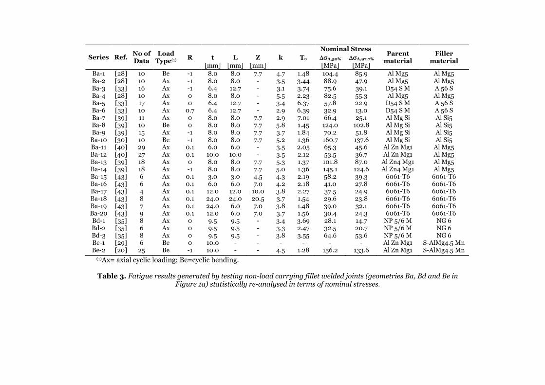
Series Ref. No of Data

Load Type(1)

R t L Z k Tσ

Nominal Stress Parent

material Filler

material ∆σA,50% ∆σA,97.7%

[mm] [mm] [mm]

[MPa] [MPa]

Ba-1 [28] 10 Be -1 8.0 8.0 7.7 4.7 1.48 104.4 85.9 Al Mg5 Al Mg5 Ba-2 [28] 10 Ax -1 8.0 8.0 - 3.5 3.44 88.9 47.9 Al Mg5 Al Mg5 Ba-3 [33] 16 Ax -1 6.4 12.7 - 3.1 3.74 75.6 39.1 D54 S M A 56 S Ba-4 [28] 10 Ax 0 8.0 8.0 - 5.5 2.23 82.5 55.3 Al Mg5 Al Mg5 Ba-5 [33] 17 Ax 0 6.4 12.7 - 3.4 6.37 57.8 22.9 D54 S M A 56 S Ba-6 [33] 10 Ax 0.7 6.4 12.7 - 2.9 6.39 32.9 13.0 D54 S M A 56 S Ba-7 [39] 11 Ax 0 8.0 8.0 7.7 2.9 7.01 66.4 25.1 Al Mg Si Al Si5 Ba-8 [39] 10 Be 0 8.0 8.0 7.7 5.8 1.45 124.0 102.8 Al Mg Si Al Si5 Ba-9 [39] 15 Ax -1 8.0 8.0 7.7 3.7 1.84 70.2 51.8 Al Mg Si Al Si5 Ba-10 [30] 10 Be -1 8.0 8.0 7.7 5.2 1.36 160.7 137.6 Al Mg Si Al Si5 Ba-11 [40] 29 Ax 0.1 6.0 6.0 - 3.5 2.05 65.3 45.6 Al Zn Mg1 Al Mg5 Ba-12 [40] 27 Ax 0.1 10.0 10.0 - 3.5 2.12 53.5 36.7 Al Zn Mg1 Al Mg5 Ba-13 [39] 18 Ax 0 8.0 8.0 7.7 5.3 1.37 101.8 87.0 Al Zn4 Mg1 Al Mg5 Ba-14 [39] 18 Ax -1 8.0 8.0 7.7 5.0 1.36 145.1 124.6 Al Zn4 Mg1 Al Mg5 Ba-15 [43] 6 Ax 0.1 3.0 3.0 4.5 4.3 2.19 58.2 39.3 6061-T6 6061-T6 Ba-16 [43] 6 Ax 0.1 6.0 6.0 7.0 4.2 2.18 41.0 27.8 6061-T6 6061-T6 Ba-17 [43] 4 Ax 0.1 12.0 12.0 10.0 3.8 2.27 37.5 24.9 6061-T6 6061-T6 Ba-18 [43] 8 Ax 0.1 24.0 24.0 20.5 3.7 1.54 29.6 23.8 6061-T6 6061-T6 Ba-19 [43] 7 Ax 0.1 24.0 6.0 7.0 3.8 1.48 39.0 32.1 6061-T6 6061-T6 Ba-20 [43] 9 Ax 0.1 12.0 6.0 7.0 3.7 1.56 30.4 24.3 6061-T6 6061-T6 Bd-1 [35] 8 Ax 0 9.5 9.5 - 3.4 3.69 28.1 14.7 NP 5/6 M NG 6 Bd-2 [35] 6 Ax 0 9.5 9.5 - 3.3 2.47 32.5 20.7 NP 5/6 M NG 6 Bd-3 [35] 8 Ax 0 9.5 9.5 - 3.8 3.55 64.6 53.6 NP 5/6 M NG 6 Be-1 [29] 6 Be 0 10.0 - - - - - - Al Zn Mg1 S-AlMg4.5 Mn Be-2 [20] 25 Be -1 10.0 - - 4.5 1.28 156.2 133.6 Al Zn Mg1 S-AlMg4.5 Mn

(1)Ax= axial cyclic loading; Be=cyclic bending.

Table 3. Fatigue results generated by testing non-load carrying fillet welded joints (geometries Ba, Bd and Be in Figure 1a) statistically re-analysed in terms of nominal stresses.

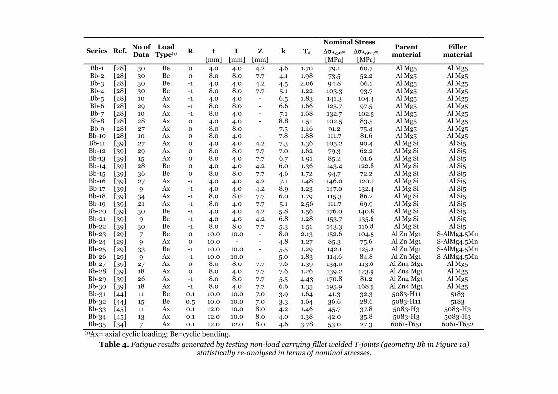
Series Ref. No of Data

Load Type(1)

R t L Z k Tσ

Nominal Stress Parent

material Filler

material ∆σA,50% ∆σA,97.7%

[mm] [mm] [mm] [MPa] [MPa]

Bb-1 [28] 30 Be 0 4.0 4.0 4.2 4.6 1.70 79.1 60.7 Al Mg5 Al Mg5 Bb-2 [28] 30 Be 0 8.0 8.0 7.7 4.1 1.98 73.5 52.2 Al Mg5 Al Mg5 Bb-3 [28] 30 Be -1 4.0 4.0 4.2 4.5 2.06 94.8 66.1 Al Mg5 Al Mg5 Bb-4 [28] 30 Be -1 8.0 8.0 7.7 5.1 1.22 103.3 93.7 Al Mg5 Al Mg5 Bb-5 [28] 10 Ax -1 4.0 4.0 - 6.5 1.83 141.3 104.4 Al Mg5 Al Mg5 Bb-6 [28] 29 Ax -1 8.0 8.0 - 6.6 1.66 125.7 97.5 Al Mg5 Al Mg5 Bb-7 [28] 10 Ax -1 8.0 4.0 - 7.1 1.68 132.7 102.5 Al Mg5 Al Mg5 Bb-8 [28] 28 Ax 0 4.0 4.0 - 8.8 1.51 102.5 83.5 Al Mg5 Al Mg5 Bb-9 [28] 27 Ax 0 8.0 8.0 - 7.5 1.46 91.2 75.4 Al Mg5 Al Mg5 Bb-10 [28] 10 Ax 0 8.0 4.0 - 7.8 1.88 111.7 81.6 Al Mg5 Al Mg5 Bb-11 [39] 27 Ax 0 4.0 4.0 4.2 7.3 1.36 105.2 90.4 Al Mg Si Al Si5 Bb-12 [39] 29 Ax 0 8.0 8.0 7.7 7.0 1.62 79.3 62.2 Al Mg Si Al Si5 Bb-13 [39] 15 Ax 0 8.0 4.0 7.7 6.7 1.91 85.2 61.6 Al Mg Si Al Si5 Bb-14 [39] 28 Be 0 4.0 4.0 4.2 6.0 1.36 143.4 122.8 Al Mg Si Al Si5 Bb-15 [39] 36 Be 0 8.0 8.0 7.7 4.6 1.72 94.7 72.2 Al Mg Si Al Si5 Bb-16 [39] 27 Ax -1 4.0 4.0 4.2 7.1 1.48 146.0 120.1 Al Mg Si Al Si5 Bb-17 [39] 9 Ax -1 4.0 4.0 4.2 8.9 1.23 147.0 132.4 Al Mg Si Al Si5 Bb-18 [39] 34 Ax -1 8.0 8.0 7.7 6.0 1.79 115.3 86.2 Al Mg Si Al Si5 Bb-19 [39] 21 Ax -1 8.0 4.0 7.7 5.1 2.56 111.7 69.9 Al Mg Si Al Si5 Bb-20 [39] 30 Be -1 4.0 4.0 4.2 5.8 1.56 176.0 140.8 Al Mg Si Al Si5 Bb-21 [39] 9 Be -1 4.0 4.0 4.2 6.8 1.28 153.7 135.6 Al Mg Si Al Si5 Bb-22 [39] 30 Be -1 8.0 8.0 7.7 5.3 1.51 143.3 116.8 Al Mg Si Al Si5 Bb-23 [29] 7 Be 0 10.0 10.0 - 8.0 2.13 152.6 104.5 Al Zn Mg1 S-AlMg4.5Mn Bb-24 [29] 9 Ax 0 10.0 - - 4.8 1.27 85.3 75.6 Al Zn Mg1 S-AlMg4.5Mn Bb-25 [29] 33 Be -1 10.0 10.0 - 5.5 1.29 142.1 125.2 Al Zn Mg1 S-AlMg4.5Mn Bb-26 [29] 9 Ax -1 10.0 10.0 - 5.0 1.83 114.6 84.8 Al Zn Mg1 S-AlMg4.5Mn Bb-27 [39] 27 Ax 0 8.0 8.0 7.7 7.6 1.39 134.0 113.6 Al Zn4 Mg1 Al Mg5 Bb-28 [39] 18 Ax 0 8.0 4.0 7.7 7.6 1.26 139.2 123.9 Al Zn4 Mg1 Al Mg5 Bb-29 [39] 26 Ax -1 8.0 8.0 7.7 5.5 4.43 170.8 81.2 Al Zn4 Mg1 Al Mg5 Bb-30 [39] 18 Ax -1 8.0 4.0 7.7 6.6 1.35 195.9 168.5 Al Zn4 Mg1 Al Mg5 Bb-31 [44] 11 Be 0.1 10.0 10.0 7.0 3.9 1.64 41.3 32.3 5083-H11 5183 Bb-32 [44] 15 Be 0.5 10.0 10.0 7.0 3.3 1.64 36.6 28.6 5083-H11 5183 Bb-33 [45] 11 Ax 0.1 12.0 10.0 8.0 4.2 1.46 45.7 37.8 5083-H3 5083-H3 Bb-34 [45] 13 Ax 0.1 12.0 10.0 8.0 4.0 1.38 42.0 35.8 5083-H3 5083-H3 Bb-35 [34] 7 Ax 0.1 12.0 12.0 8.0 4.6 3.78 53.0 27.3 6061-T651 6061-T652

(1)Ax= axial cyclic loading; Be=cyclic bending.

Table 4. Fatigue results generated by testing non-load carrying fillet welded T-joints (geometry Bb in Figure 1a) statistically re-analysed in terms of nominal stresses.

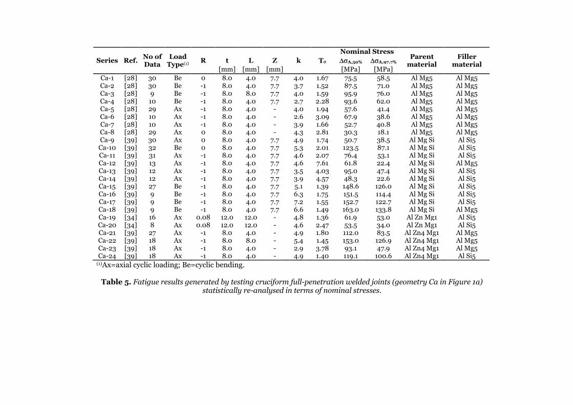
Series Ref. No of Data

Load Type(1)

R t L Z k Tσ

Nominal Stress Parent

material Filler

material ∆σA,50% ∆σA,97.7%

[mm] [mm] [mm] [MPa] [MPa]

Ca-1 [28] 30 Be 0 8.0 4.0 7.7 4.0 1.67 75.5 58.5 Al Mg5 Al Mg5 Ca-2 [28] 30 Be -1 8.0 4.0 7.7 3.7 1.52 87.5 71.0 Al Mg5 Al Mg5 Ca-3 [28] 9 Be -1 8.0 8.0 7.7 4.0 1.59 95.9 76.0 Al Mg5 Al Mg5 Ca-4 [28] 10 Be -1 8.0 4.0 7.7 2.7 2.28 93.6 62.0 Al Mg5 Al Mg5 Ca-5 [28] 29 Ax -1 8.0 4.0 - 4.0 1.94 57.6 41.4 Al Mg5 Al Mg5 Ca-6 [28] 10 Ax -1 8.0 4.0 - 2.6 3.09 67.9 38.6 Al Mg5 Al Mg5 Ca-7 [28] 10 Ax -1 8.0 4.0 - 3.9 1.66 52.7 40.8 Al Mg5 Al Mg5 Ca-8 [28] 29 Ax 0 8.0 4.0 - 4.3 2.81 30.3 18.1 Al Mg5 Al Mg5 Ca-9 [39] 30 Ax 0 8.0 4.0 7.7 4.9 1.74 50.7 38.5 Al Mg Si Al Si5 Ca-10 [39] 32 Be 0 8.0 4.0 7.7 5.3 2.01 123.5 87.1 Al Mg Si Al Si5 Ca-11 [39] 31 Ax -1 8.0 4.0 7.7 4.6 2.07 76.4 53.1 Al Mg Si Al Si5 Ca-12 [39] 13 Ax -1 8.0 4.0 7.7 4.6 7.61 61.8 22.4 Al Mg Si Al Mg5 Ca-13 [39] 12 Ax -1 8.0 4.0 7.7 3.5 4.03 95.0 47.4 Al Mg Si Al Si5 Ca-14 [39] 12 Ax -1 8.0 4.0 7.7 3.9 4.57 48.3 22.6 Al Mg Si Al Si5 Ca-15 [39] 27 Be -1 8.0 4.0 7.7 5.1 1.39 148.6 126.0 Al Mg Si Al Si5 Ca-16 [39] 9 Be -1 8.0 4.0 7.7 6.3 1.75 151.5 114.4 Al Mg Si Al Si5 Ca-17 [39] 9 Be -1 8.0 4.0 7.7 7.2 1.55 152.7 122.7 Al Mg Si Al Si5 Ca-18 [39] 9 Be -1 8.0 4.0 7.7 6.6 1.49 163.0 133.8 Al Mg Si Al Mg5 Ca-19 [34] 16 Ax 0.08 12.0 12.0 - 4.8 1.36 61.9 53.0 Al Zn Mg1 Al Si5 Ca-20 [34] 8 Ax 0.08 12.0 12.0 - 4.6 2.47 53.5 34.0 Al Zn Mg1 Al Si5 Ca-21 [39] 27 Ax -1 8.0 4.0 - 4.9 1.80 112.0 83.5 Al Zn4 Mg1 Al Mg5 Ca-22 [39] 18 Ax -1 8.0 8.0 - 5.4 1.45 153.0 126.9 Al Zn4 Mg1 Al Mg5 Ca-23 [39] 18 Ax -1 8.0 4.0 - 2.9 3.78 93.1 47.9 Al Zn4 Mg1 Al Mg5 Ca-24 [39] 18 Ax -1 8.0 4.0 - 4.9 1.40 119.1 100.6 Al Zn4 Mg1 Al Si5

(1)Ax=axial cyclic loading; Be=cyclic bending.

Table 5. Fatigue results generated by testing cruciform full-penetration welded joints (geometry Ca in Figure 1a) statistically re-analysed in terms of nominal stresses.

Series Ref. No of Data

Load Type(1)

R t L Z k Tσ

Nominal Stress Parent

material Filler

material ∆σA,50% ∆σA,97.7%

[mm] [mm] [mm]

[MPa] [MPa]

Cb-1 [28] 27 Ax -1 4.0 4.0 - 4.8 1.86 84.8 62.2 Al Mg5 Al Mg5 Cb-2 [28] 29 Ax -1 8.0 8.0 - 3.8 1.77 69.3 52.1 Al Mg5 Al Mg5 Cb-3 [33] 9 Ax -1 6.4 12.7 - 4.5 2.41 75.9 48.9 D54 S M A 56 S Cb-4 [28] 27 Ax 0 4.0 4.0 - 4.8 2.16 54.3 37.0 Al Mg5 Al Mg5 Cb-5 [28] 30 Ax 0 8.0 8.0 - 4.3 1.88 39.5 28.8 Al Mg5 Al Mg5 Cb-6 [33] 20 Ax 0 6.4 12.7 - 5.0 4.61 49.6 23.1 D54 S M A 56 S Cb-7 [33] 25 Ax 0 10.0 10.0 - 3.4 1.26 28.6 25.5 Al Mg5 F28 S-AlMg4.5Mn Cb-8 [33] 10 Ax 0.6 6.4 12.7 - 5.0 1.83 42.5 31.4 D54 S M A 56 S Cb-9 [33] 6 Ax 0.75 6.4 12.7 - 2.9 2.38 33.7 21.9 D54 S M A 56 S Cb-10 [39] 31 Ax 0 4.0 4.0 4.2 6.0 1.84 72.0 53.1 Al Mg Si Al Si5 Cb-11 [39] 23 Ax 0 8.0 8.0 7.7 6.0 1.49 50.2 41.1 Al Mg Si Al Si5 Cb-12 [39] 25 Ax 0 8.0 8.0 7.7 5.9 1.51 42.9 34.9 Al Mg Si Al Si5 Cb-13 [39] 27 Ax -1 4.0 4.0 4.2 6.5 1.76 114.2 86.0 Al Mg Si Al Si5 Cb-14 [39] 11 Ax -1 4.0 8.0 4.2 5.8 2.47 105.1 66.9 Al Mg Si Al Si5 Cb-15 [39] 28 Ax -1 8.0 8.0 7.7 4.4 1.98 66.9 47.5 Al Mg Si Al Si5 Cb-16 [34] 12 Ax 0.08 12.0 12.0 6.3 5.8 1.40 38.9 32.9 Al Zn Mg1 Al Si5 Cb-17 [34] 14 Ax 0.08 12.0 12.0 6.3 4.6 1.36 36.2 31.0 Al Zn Mg1 Al Si5 Cb-18 [40] 29 Ax 0.1 6.0 6.0 - 5.3 1.77 54.9 41.2 Al Zn Mg1 Al Si5 Cb-19 [39] 27 Ax 0 4.0 4.0 4.2 3.5 1.86 65.9 48.3 Al Zn4 Mg1 Al Mg5 Cb-20 [39] 27 Ax 0 8.0 8.0 7.7 4.2 2.14 50.0 34.2 Al Zn4 Mg1 Al Mg5 Cb-21 [39] 18 Ax 0 8.0 - - 4.1 2.32 43.5 28.6 Al Zn4 Mg1 Al Mg5 Cb-22 [39] 27 Ax -1 8.0 8.0 7.7 3.5 3.43 92.3 49.8 Al Zn4 Mg1 Al Mg5 Cb-23 [42] 12 Ax 0.1 12.0 12.0 8.0 5.3 2.17 29.5 20.0 6061-T651 6061-T652 Cb-24 [42] 18 Ax 0.1 12.0 12.0 6.4 4.4 1.47 27.4 22.6 Al Zn Mg1 Al Zn Mg2 Cc-1 [39] 30 Be 0 4.0 8.0 - 4.7 1.83 119.4 88.3 Al Mg Si Al Si5 Cc-2 [39] 11 Be 0 4.0 8.0 - 5.5 1.78 133.8 100.3 Al Mg Si Al Si5 Cc-3 [39] 28 Be 0 8.0 8.0 - 3.9 1.66 92.8 72.0 Al Mg Si Al Si5 Cc-4 [39] 29 Be -1 4.0 8.0 - 4.1 1.55 144.4 116.1 Al Mg Si Al Si5 Cc-5 [39] 12 Be -1 4.0 8.0 - 6.5 1.42 165.1 138.6 Al Mg Si Al Si5

(1)Ax=axial cyclic loading; Be=cyclic bending.

Table 6. Fatigue results generated by testing load carrying fillet cruciform welded joints (geometry Cb in Figure 1a) statistically re-analysed in terms of nominal stresses.

Approach Welded

Geometry

Nominal Stress EC9 IIW

∆σA,50%(1) ∆σA,97.7%

(2) k Tσ

(3) ∆σA,97.7%

k ∆σA,95%

k [MPa] [MPa] [MPa] [MPa]

Nominal Stress

Aa 72.1 13.0 1.8 30.88 55 4.5 45 3

Ab 65.0 17.3 2.4 14.21 36 4.3 36 3

Ae 185.3 89.2 7.0 4.32 55 4.5 45 3

Ba 45.7 15.5 2.1 8.69 23 3.4 36 3

Bb 73.3 22.6 2.5 10.53 23 3.4 36 3

Bd 30.8 6.5 2.0 22.31 23 3.4 36 3

Be 54.5 7.6 1.9 51.79 23 3.4 36 3

Ca 40.1 6.6 1.8 36.60 36 3.4 32 3

Cb 36.3 11.6 2.7 9.81 25 3.4 36 3

Cc 109.8 67.2 3.8 2.67 25 3.4 36 3

Hot-Spot Stress

Ba 51.2 13.3 1.9 14.87 - - 40 3

Bb 75.8 20.1 2.2 14.30 - - 40 3

Ca 65.4 17.3 2.2 14.36 - - 40 3

Cb 40.7 11.4 2.4 12.67 - - 36 3

Effective Notch Stress

Ba≥5 113.2 35.1 2.0 10.40 - - 71 3

Ba<5 314.6 85.1 4.3 2.13 - - 180 3

Bb≥5 145.7 33.3 2.0 19.17 - - 71 3

Bb<5 218.9 85.9 3.1 6.50 - - 180 3

Ca≥5 129.8 34.0 2.2 14.55 - - 71 3

Cb≥5 121.3 40.8 2.7 8.83 - - 71 3

Cb<5 297.9 26.2 2.5 20.05 - - 180 3

N-SIF

Ba 119.5 43.7 2.3 7.46 - - - -

Bb 150.4 34.9 2.1 18.57 - - - -

Ca 112.0 21.6 1.9 26.91 - - - -

Cb 120.7 48.9 3.0 6.09 - - - -

TCD

Ba 80.0 29.0 2.3 7.62 - - - -

Bb 88.5 16.8 1.8 27.74 - - - -

Ca 89.2 23.4 2.2 14.60 - - - -

Cb 81.4 33.0 3.0 6.09 - - - -

(1)∆KI,50% at 2∙106 cycles to failure for the N-SIF approach measured in units of MPa∙mm0.326. (2)∆KI,97.7% at 2∙106 cycles to failure for the N-SIF approach measured in units of MPa∙mm0.326. (3)Tσ=∆KI,90%/∆KI,10% for the N-SIF approach.

Table 7. Summary of the statistical re-analyses for the different approaches/welded geometries

and corresponding recommended curves.

Series Ref. No of Data

Load Type(1)

R t L Z

k Tσ(2)

Hot-Spot Stress Effective Notch

Stress N-SIF TCD

∆σA,50% ∆σA,97.7% ∆σA,50% ∆σA,97.7% ∆KI,50% ∆KI,97.7% ∆σA,50% ∆σA,97.7%

[mm] [mm] [mm] [MPa] [MPa] [MPa] [MPa] [MPa∙mm0.326] [MPa∙mm0.326] [MPa] [MPa]

Ba-1 [28] 10 Be -1 8.0 8.0 7.7 4.7 1.48 129.8 106.8 244.3 200.9 184.8 152.0 124.6 102.5 Ba-7 [39] 11 Ax 0 8.0 8.0 7.7 2.9 7.01 76.4 28.9 155.3 58.6 156.4 59.1 105.5 39.8 Ba-8 [39] 10 Be 0 8.0 8.0 7.7 5.8 1.45 142.6 118.3 290.0 240.5 219.7 182.2 148.1 122.9 Ba-9 [39] 15 Ax -1 8.0 8.0 7.7 3.7 1.84 80.8 59.6 164.3 121.1 165.5 122.0 111.6 82.3 Ba-10 [39] 10 Be -1 8.0 8.0 7.7 5.2 1.36 184.9 158.3 375.9 321.9 284.8 243.9 192.0 164.4 Ba-13 [39] 18 Ax 0 8.0 8.0 7.7 5.3 1.37 126.6 108.2 238.2 203.6 240.0 205.1 161.8 138.3 Ba-14 [39] 18 Ax -1 8.0 8.0 7.7 5.0 1.36 180.4 154.9 339.4 291.4 342.0 293.6 230.6 197.9 Ba-15 [43] 6 Ax 0.1 3.0 3.0 4.5 4.3 2.19 81.9 55.3 124.1 83.8 124.7 84.2 84.4 57.0 Ba-16 [43] 6 Ax 0.1 6.0 6.0 7.0 4.2 2.18 58.4 39.6 110.6 75.0 110.2 74.7 75.1 49.1 Ba-17 [43] 4 Ax 0.1 12.0 12.0 10.0 3.8 2.27 55.1 36.6 125.9 83.6 127.5 84.7 86.0 57.1 Ba-18 [43] 8 Ax 0.1 24.0 24.0 20.5 3.7 1.54 43.6 35.0 124.5 100.2 126.7 101.9 85.6 68.9 Ba-19 [43] 7 Ax 0.1 24.0 6.0 7.0 3.8 1.48 56.2 46.3 125.0 102.9 127.4 104.9 85.9 70.7 Ba-20 [43] 9 Ax 0.1 12.0 6.0 7.0 3.7 1.56 45.2 36.2 94.9 75.9 96.7 77.3 63.5 50.8

(1)Ax=axial cyclic loading; Be=cyclic bending; (2)Tσ=∆KI,90%/∆KI,10% for the N-SIF approach.

Table 8. Fatigue results generated by testing non-load carrying fillet cruciform welded joints (geometry Ba in Figure 1a) statistically re-analysed in terms of hot-spot stresses as well as in terms of local stress quantities.

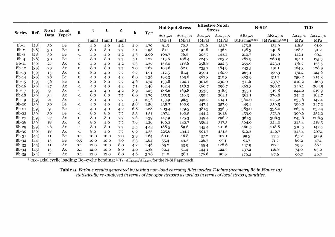
Series Ref. No of Data

Load Type(1)

R t L Z

k Tσ(2)

Hot-Spot Stress Effective Notch

Stress N-SIF TCD

∆σA,50% ∆σA,97.7% ∆σA,50% ∆σA,97.7% ∆KI,50% ∆KI,97.7% ∆σA,50% ∆σA,97.7%

[mm] [mm] [mm] [MPa] [MPa] [MPa] [MPa] [MPa∙mm0.326] [MPa∙mm0.326] [MPa] [MPa]

Bb-1 [28] 30 Be 0 4.0 4.0 4.2 4.6 1.70 91.5 70.3 171.6 131.7 175.8 134.9 118.5 91.0 Bb-2 [28] 30 Be 0 8.0 8.0 7.7 4.1 1.98 81.1 57.6 191.8 136.2 198.3 140.8 128.4 91.2 Bb-3 [28] 30 Be -1 4.0 4.0 4.2 4.5 2.06 109.7 76.5 205.7 143.4 210.7 146.9 142.1 99.1 Bb-4 [28] 30 Be -1 8.0 8.0 7.7 5.1 1.22 119.6 108.4 224.2 203.2 287.9 260.9 194.1 175.9 Bb-11 [39] 27 Ax 0 4.0 4.0 4.2 7.3 1.36 138.0 118.6 258.8 222.3 259.9 223.3 178.7 153.5 Bb-12 [39] 29 Ax 0 8.0 8.0 7.7 7.0 1.62 104.6 82.0 235.7 184.9 243.5 191.1 164.3 128.9 Bb-13 [39] 15 Ax 0 8.0 4.0 7.7 6.7 1.91 112.5 81.4 250.1 180.9 263.1 190.3 172.2 124.6 Bb-14 [39] 28 Be 0 4.0 4.0 4.2 6.0 1.36 193.3 165.6 362.3 310.3 363.9 311.7 250.2 214.3 Bb-15 [39] 36 Be 0 8.0 8.0 7.7 4.6 1.72 133.8 102.1 301.6 230.0 311.6 237.7 210.2 160.3 Bb-16 [39] 27 Ax -1 4.0 4.0 4.2 7.1 1.48 192.4 158.3 360.7 296.7 362.3 298.0 249.1 204.9 Bb-17 [39] 9 Ax -1 4.0 4.0 4.2 8.9 1.23 188.6 169.8 353.5 318.3 355.1 319.8 244.2 219.9 Bb-18 [39] 34 Ax -1 8.0 8.0 7.7 6.0 1.79 155.5 116.3 350.4 262.1 362.1 270.8 244.2 182.7 Bb-19 [39] 21 Ax -1 8.0 4.0 7.7 5.1 2.56 153.9 96.3 342.2 214.1 360.0 225.2 235.6 147.4 Bb-20 [39] 30 Be -1 4.0 4.0 4.2 5.8 1.56 238.7 190.9 447.4 357.9 449.4 359.5 309.0 247.2 Bb-21 [39] 9 Be -1 4.0 4.0 4.2 6.8 1.28 203.4 179.5 381.3 336.5 383.0 338.0 263.4 232.4 Bb-22 [39] 30 Be -1 8.0 8.0 7.7 5.3 1.51 197.1 160.5 444.2 361.8 459.0 373.9 309.6 252.2 Bb-27 [39] 27 Ax 0 8.0 8.0 7.7 7.6 1.39 147.9 125.3 349.4 296.2 361.3 306.3 243.6 206.5 Bb-28 [39] 18 Ax 0 8.0 4.0 7.7 7.6 1.26 160.3 142.7 356.4 317.3 364.0 324.0 245.4 218.5 Bb-29 [39] 26 Ax -1 8.0 8.0 7.7 5.5 4.43 188.5 89.6 445.4 211.6 460.5 218.8 310.5 147.5 Bb-30 [39] 18 Ax -1 8.0 4.0 7.7 6.6 1.35 225.6 194.1 501.7 431.5 512.3 440.7 345.4 297.1 Bb-31 [44] 11 Be 0.1 10.0 10.0 7.0 3.9 1.64 60.0 46.8 137.2 107.1 99.3 77.5 65.2 50.9 Bb-32 [44] 15 Be 0.5 10.0 10.0 7.0 3.3 1.64 55.4 43.3 126.7 99.1 91.7 71.7 60.2 47.1 Bb-33 [45] 11 Ax 0.1 12.0 10.0 8.0 4.2 1.46 65.2 53.9 155.4 128.6 147.9 122.4 79.9 66.1 Bb-34 [45] 13 Ax 0.1 12.0 10.0 8.0 4.0 1.38 60.4 51.4 144.1 122.7 137.2 116.8 74.0 63.0 Bb-35 [34] 7 Ax 0.1 12.0 12.0 8.0 4.6 3.78 74.0 38.1 176.6 90.9 170.2 87.6 90.7 46.7

(1)Ax=axial cyclic loading; Be=cyclic bending; (2)Tσ=∆KI,90%/∆KI,10% for the N-SIF approach.

Table 9. Fatigue results generated by testing non-load carrying fillet welded T-joints (geometry Bb in Figure 1a) statistically re-analysed in terms of hot-spot stresses as well as in terms of local stress quantities.

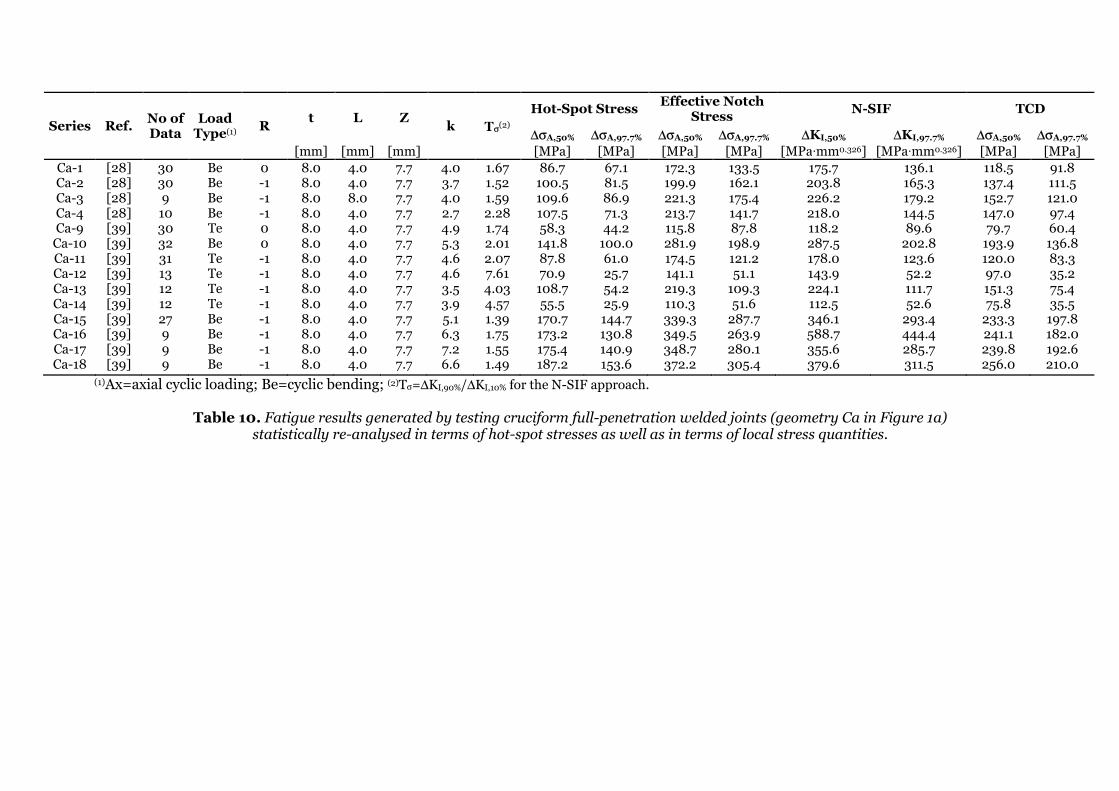
Series Ref. No of Data

Load Type(1)

R t L Z

k Tσ(2)

Hot-Spot Stress Effective Notch

Stress N-SIF TCD

∆σA,50% ∆σA,97.7% ∆σA,50% ∆σA,97.7% ∆KI,50% ∆KI,97.7% ∆σA,50% ∆σA,97.7%

[mm] [mm] [mm] [MPa] [MPa] [MPa] [MPa] [MPa∙mm0.326] [MPa∙mm0.326] [MPa] [MPa]

Ca-1 [28] 30 Be 0 8.0 4.0 7.7 4.0 1.67 86.7 67.1 172.3 133.5 175.7 136.1 118.5 91.8 Ca-2 [28] 30 Be -1 8.0 4.0 7.7 3.7 1.52 100.5 81.5 199.9 162.1 203.8 165.3 137.4 111.5 Ca-3 [28] 9 Be -1 8.0 8.0 7.7 4.0 1.59 109.6 86.9 221.3 175.4 226.2 179.2 152.7 121.0 Ca-4 [28] 10 Be -1 8.0 4.0 7.7 2.7 2.28 107.5 71.3 213.7 141.7 218.0 144.5 147.0 97.4 Ca-9 [39] 30 Te 0 8.0 4.0 7.7 4.9 1.74 58.3 44.2 115.8 87.8 118.2 89.6 79.7 60.4 Ca-10 [39] 32 Be 0 8.0 4.0 7.7 5.3 2.01 141.8 100.0 281.9 198.9 287.5 202.8 193.9 136.8 Ca-11 [39] 31 Te -1 8.0 4.0 7.7 4.6 2.07 87.8 61.0 174.5 121.2 178.0 123.6 120.0 83.3 Ca-12 [39] 13 Te -1 8.0 4.0 7.7 4.6 7.61 70.9 25.7 141.1 51.1 143.9 52.2 97.0 35.2 Ca-13 [39] 12 Te -1 8.0 4.0 7.7 3.5 4.03 108.7 54.2 219.3 109.3 224.1 111.7 151.3 75.4 Ca-14 [39] 12 Te -1 8.0 4.0 7.7 3.9 4.57 55.5 25.9 110.3 51.6 112.5 52.6 75.8 35.5 Ca-15 [39] 27 Be -1 8.0 4.0 7.7 5.1 1.39 170.7 144.7 339.3 287.7 346.1 293.4 233.3 197.8 Ca-16 [39] 9 Be -1 8.0 4.0 7.7 6.3 1.75 173.2 130.8 349.5 263.9 588.7 444.4 241.1 182.0 Ca-17 [39] 9 Be -1 8.0 4.0 7.7 7.2 1.55 175.4 140.9 348.7 280.1 355.6 285.7 239.8 192.6 Ca-18 [39] 9 Be -1 8.0 4.0 7.7 6.6 1.49 187.2 153.6 372.2 305.4 379.6 311.5 256.0 210.0

(1)Ax=axial cyclic loading; Be=cyclic bending; (2)Tσ=∆KI,90%/∆KI,10% for the N-SIF approach.

Table 10. Fatigue results generated by testing cruciform full-penetration welded joints (geometry Ca in Figure 1a) statistically re-analysed in terms of hot-spot stresses as well as in terms of local stress quantities.

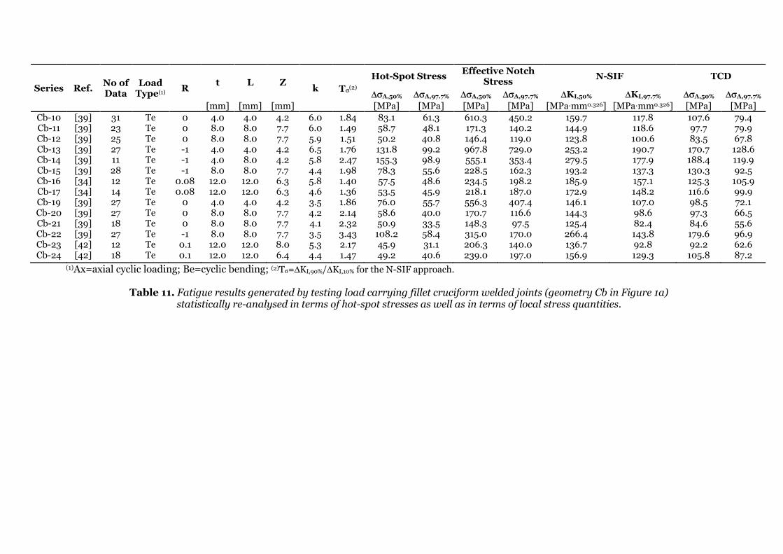
Series Ref. No of Data

Load Type(1)

R t L Z

k Tσ(2)

Hot-Spot Stress Effective Notch

Stress N-SIF TCD

∆σA,50% ∆σA,97.7% ∆σA,50% ∆σA,97.7% ∆KI,50% ∆KI,97.7% ∆σA,50% ∆σA,97.7%

[mm] [mm] [mm] [MPa] [MPa] [MPa] [MPa] [MPa∙mm0.326] [MPa∙mm0.326] [MPa] [MPa]

Cb-10 [39] 31 Te 0 4.0 4.0 4.2 6.0 1.84 83.1 61.3 610.3 450.2 159.7 117.8 107.6 79.4 Cb-11 [39] 23 Te 0 8.0 8.0 7.7 6.0 1.49 58.7 48.1 171.3 140.2 144.9 118.6 97.7 79.9 Cb-12 [39] 25 Te 0 8.0 8.0 7.7 5.9 1.51 50.2 40.8 146.4 119.0 123.8 100.6 83.5 67.8 Cb-13 [39] 27 Te -1 4.0 4.0 4.2 6.5 1.76 131.8 99.2 967.8 729.0 253.2 190.7 170.7 128.6 Cb-14 [39] 11 Te -1 4.0 8.0 4.2 5.8 2.47 155.3 98.9 555.1 353.4 279.5 177.9 188.4 119.9 Cb-15 [39] 28 Te -1 8.0 8.0 7.7 4.4 1.98 78.3 55.6 228.5 162.3 193.2 137.3 130.3 92.5 Cb-16 [34] 12 Te 0.08 12.0 12.0 6.3 5.8 1.40 57.5 48.6 234.5 198.2 185.9 157.1 125.3 105.9 Cb-17 [34] 14 Te 0.08 12.0 12.0 6.3 4.6 1.36 53.5 45.9 218.1 187.0 172.9 148.2 116.6 99.9 Cb-19 [39] 27 Te 0 4.0 4.0 4.2 3.5 1.86 76.0 55.7 556.3 407.4 146.1 107.0 98.5 72.1 Cb-20 [39] 27 Te 0 8.0 8.0 7.7 4.2 2.14 58.6 40.0 170.7 116.6 144.3 98.6 97.3 66.5 Cb-21 [39] 18 Te 0 8.0 8.0 7.7 4.1 2.32 50.9 33.5 148.3 97.5 125.4 82.4 84.6 55.6 Cb-22 [39] 27 Te -1 8.0 8.0 7.7 3.5 3.43 108.2 58.4 315.0 170.0 266.4 143.8 179.6 96.9 Cb-23 [42] 12 Te 0.1 12.0 12.0 8.0 5.3 2.17 45.9 31.1 206.3 140.0 136.7 92.8 92.2 62.6 Cb-24 [42] 18 Te 0.1 12.0 12.0 6.4 4.4 1.47 49.2 40.6 239.0 197.0 156.9 129.3 105.8 87.2

(1)Ax=axial cyclic loading; Be=cyclic bending; (2)Tσ=∆KI,90%/∆KI,10% for the N-SIF approach.

Table 11. Fatigue results generated by testing load carrying fillet cruciform welded joints (geometry Cb in Figure 1a) statistically re-analysed in terms of hot-spot stresses as well as in terms of local stress quantities.

∆σA,50%(1) ∆KI,50%

(1) t=L=Z ∆σnom,50%(1) LW-Al

[MPa] [MPa∙mm0.326] [mm] [MPa] [mm]

79.2 124.5

8 52.7 0.50

12 46.2 0.49

16 42.1 0.49

20 39.1 0.48 (1)at 2∙106 cycles to failure

Table 12. Influence of the welded joint’s absolute dimensions on the estimated value for LW-Al.

n q

PS=90%-10% PS=95%-5% PS=99%-1%

3 6.158 7.655 10.552

4 4.163 5.145 7.042

5 3.407 4.202 5.741

6 3.006 3.707 5.062

7 2.755 3.399 4.641

8 2.582 3.188 4.353

9 2.454 3.031 4.143

10 2.355 2.911 3.981

11 2.275 2.815 3.852

12 2.210 2.736 3.747

13 2.155 2.670 3.659

14 2.108 2.614 3.585

15 2.068 2.566 3.520

16 2.032 2.523 3.463

17 2.001 2.486 3.415

18 1.974 2.453 3.370

19 1.949 2.423 3.331

20 1.926 2.396 3.295

21 1.905 2.371 3.262

22 1.887 2.350 3.233

23 1.869 2.329 3.206

24 1.853 2.309 3.181

25 1.838 2.292 3.158

30 1.778 2.220 3.064

35 1.732 2.166 2.994

40 1.697 2.126 2.941

45 1.669 2.092 2.897

50 1.646 2.065 2.863

Table A1. Index q for a confidence level equal to 0.95% [67].

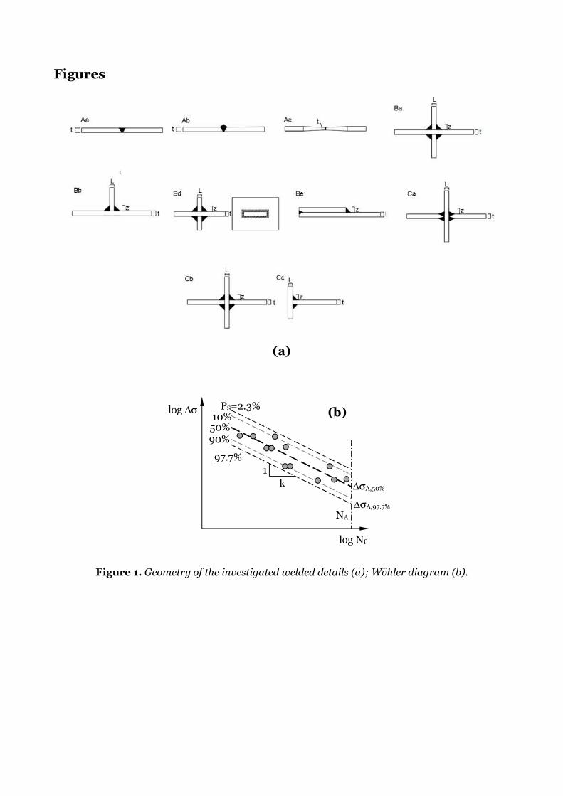
Figures

(a)

Figure 1. Geometry of the investigated welded details (a); Wöhler diagram (b).

(b) log ∆σ

log Nf

NA

k

1

PS=2.3%

10%

50%

90%

97.7%

∆σA,50%

∆σA,97.7%

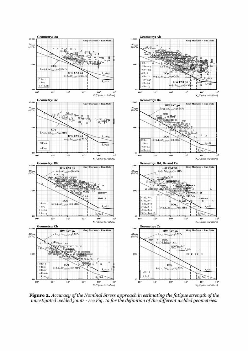
Figure 2. Accuracy of the Nominal Stress approach in estimating the fatigue strength of the investigated welded joints - see Fig. 1a for the definition of the different welded geometries.

10

100

1000

1000 10000 100000 1000000 10000000 100000000

∆σnom

[MPa]

Nf [Cycles to Failure]

Geometry: Aa

R=-1

R=0

R=0.08

Grey Markers = Run Outs

IIW FAT 45

k=3, ∆σA,95%=45 MPa

103 104 105 106 107 108

EC9

k=4.5, ∆σA,97.7%=55 MPa

k2=6.5

k2=22

10

100

1000

1000 10000 100000 1000000 10000000 100000000

∆σnom

[MPa]

Nf [Cycles to Failure]

Geometry: Ab

R=-1

R=-0.4

R=-0.2

R=0

R≈0.1

R≈0.25

R=0.4

R≈0.5

Grey Markers = Run Outs

IIW FAT 36

k=3, ∆σA,95%=36 MPa

103 104 105 106 107 108

EC9

k=4.3, ∆σA97.7%=36 MPak2=6.3

k2=22

10

100

1000

1000 10000 100000 1000000 10000000 100000000

∆σnom

[MPa]

Nf [Cycles to Failure]

Geometry: Ae

R=-1

R=0

Grey Markers = Run Outs

IIW FAT 45

k=3, ∆σA95%=45 MPa

103 104 105 106 107 108

EC9

k=4.5, ∆σA97.7%=55 MPa

k2=6.5

k2=22

10

100

1000

1000 10000 100000 1000000 10000000 100000000

∆σnom

[MPa]

Nf [Cycles to Failure]

Geometry: Ba

R=-1

R=0

R=0.1

R=0.7

Grey Markers = Run OutsIIW FAT 36

k=3, ∆σA,95%=36 MPa

103 104 105 106 107 108

EC9

k=3.4, ∆σA,97.7%=23 MPa

k2=5.4

k2=22

10

100

1000

1000 10000 100000 1000000 10000000 100000000

∆σnom

[MPa]

Nf [Cycles to Failure]

Geometry: Bb

R=-1

R=0

R=0.1

R=0.5

Grey Markers = Run OutsIIW FAT 36

k=3, ∆σA,95%=36 MPa

103 104 105 106 107 108

EC9

k=3.4, ∆σA,97.7%=23 MPa

k2=5.4

k2=22

10

100

1000

1000 10000 100000 1000000 10000000 100000000

∆σnom

[MPa]

Nf [Cycles to Failure]

Geometry: Bd, Be and Ca

Bd, R=0

Be, R=-1

Be, R=0

Ca, R=-1

Ca, R=0

Ca, R=0.08

Grey Markers = Run OutsIIW FAT 36

k=3, ∆σA,95%=36 MPa

103 104 105 106 107 108

EC9

k=3.4, ∆σA,97.7%=23 MPa

k2=5.4

k2=22

10

100

1000

1000 10000 100000 1000000 10000000 100000000

∆σnom

[MPa]

Nf [Cycles to Failure]

Geometry: Cb

R=-1

R=0

R≈0.1

R=0.6

R=0.75

Grey Markers = Run OutsIIW FAT 36

k=3, ∆σA,95%=36 MPa

103 104 105 106 107 108

EC9

k=3.4, ∆σA,97.7%=23 MPa

k2=5.4

k2=22

10

100

1000

1000 10000 100000 1000000 10000000 100000000

∆σnom

[MPa]

Nf [Cycles to Failure]

Geometry: Cc

R=-1

R=0

Grey Markers = Run OutsIIW FAT 36

k=3, ∆σA,95%=36 MPa

103 104 105 106 107 108

EC9

k=3.4, ∆σA,97.7%=23 MPa

k2=5.4

k2=22

(a)

(b)

Figure 3. Definition of hot-spot stress (a); accuracy of the Hot-Spot Stress approach in estimating the fatigue strength of the investigated welded joints (b) - see Fig. 1a for the definition

of the different welded geometries.

10

100

1000

1000 10000 100000 1000000 10000000 100000000

∆σHS

[MPa]

Nf [Cycles to Failure]

Geometry: Ba

R=-1

R=0

R=0.1

IIW FAT 40

k=3, ∆σA,95%=40 MPa

103 104 105 106 107 108

k2=22

10

100

1000

1000 10000 100000 1000000 10000000 100000000

∆σHS

[MPa]

Nf [Cycles to Failure]

Geometry: Bb

R=-1

R=0

R=0.1

R=0.5

Grey Markers = Run Outs

IIW FAT 40

k=3, ∆σA,95%=40 MPa

103 104 105 106 107 108

k2=22

10

100

1000

1000 10000 100000 1000000 10000000 100000000

∆σHS

[MPa]

Nf [Cycles to Failure]

Geometry: Ca

R=-1

R=0

Grey Markers = Run Outs

IIW FAT 40

k=3, ∆σA,95%=40 MPa

103 104 105 106 107 108

k2=22

10

100

1000

1000 10000 100000 1000000 10000000 100000000

∆σHS

[MPa]

Nf [Cycles to Failure]

Geometry: Cb

R=-1

R=0

R=0.081

R=0.1

Grey Markers = Run Outs

IIW FAT 36

k=3, ∆σA,95%=36 MPa

103 104 105 106 107 108

k2=22

Stress

0.4t t

∆σHS ∆σ0.4t

∆σt

Distance

Stress distribution on surface

∆σHS=1.67∙∆σ0.4t-0.67∙∆σt

∆σnom

t

Figure 4. Examples of FE models being solved.

(a)

(b)

(c)

(a)

(b)

Figure 5. Weld toe and root rounded according to the reference radius concept (a); accuracy of the Effective Notch Stress approach in estimating the fatigue strength of the investigated welded

joints (b) - see Fig. 1a for the definition of the different welded geometries.

0.1

1

10

100

1000 10000 100000 1000000 10000000 100000000

∆σ

NS/ ∆

σA

,95

%

Nf [Cycles to Failure]

Geometry: Ba

R=-1, t≥5 mm

R=0, t≥5 mm

R=0.1, t≥5 mm

R=0, t<5 mm

FAT 71/180

k=3, ∆σA,95%=71 MPa for t≥5 mm

k=3, ∆σA,95%=180 MPa for t<5 mm

103 104 105 106 107 108

k2=22

0.1

1

10

100

1000 10000 100000 1000000 10000000 100000000

∆σ

NS/ ∆

σA

,95

%

Nf [Cycles to Failure]

Geometry: Bb

R=-1, t≥5 mm

R=0, t≥5 mm

R=0.1, t≥5 mm

R=0.5, t≥5 mm

R=-1, t<5 mm

R=0, t<5 mm

Grey Markers = Run OutsFAT 71/180

k=3, ∆σA,95%=71 MPa for t≥5 mm

k=3, ∆σA,95%=180 MPa for t<5 mm

103 104 105 106 107 108

k2=22

0.1

1

10

100

1000 10000 100000 1000000 10000000 100000000

∆σ

NS/ ∆

σA

,95

%

Nf [Cycles to Failure]

Geometry: Ca

R=-1, t≥5 mm

R=0, t≥5 mm

Grey Markers = Run OutsFAT 71/180

k=3, ∆σA,95%=71 MPa for t≥5 mm

k=3, ∆σA,95%=180 MPa for t<5 mm

103 104 105 106 107 108

k2=22

0.1

1

10

100

1000 10000 100000 1000000 10000000 100000000

∆σ

NS/ ∆

σA

,95

%

Nf [Cycles to Failure]

Geometry: Cb

R=-1, t≥5 mm

R=0, t≥5 mm

R=0.081, t≥5 mm

R=0.1, t≥5 mm

R=-1, t<5 mm

R=0, t<5 mm

Grey Markers = Run OutsFAT 71/180

k=3, ∆σA,95%=71 MPa for t≥5 mm

k=3, ∆σA,95%=180 MPa for t<5 mm

103 104 105 106 107 108

k2=22

∆σnom

rref

rref

rref

t≥5 mm ⇒ rref=1 mm

t<5 mm ⇒ rref=0.05 mm

t

(a)

(b)

Figure 6. Local stress state in the vicinity of the weld toe (a); accuracy of the N-SIF approach in estimating the fatigue strength of the investigated welded joints (b) - see Fig. 1a for the definition

of the different welded geometries.

10

100

1000

1000 10000 100000 1000000 10000000 100000000

∆K

I[M

Pa

∙mm

0.3

26]

Nf [Cycles to Failure]

Geometry: Ba

R=-1

R=0

R=0.1

Master Curve

k=4, ∆ΚI,97.7%=74 MPa∙mm0.326

103 104 105 106 107 108

10

100

1000

1000 10000 100000 1000000 10000000 100000000

∆K

I[M

Pa

∙mm

0.3

26]

Nf [Cycles to Failure]

Geometry: Bb

R=-1

R=0

R=0.1

R=0.5

Grey Markers = Run Outs

103 104 105 106 107 108

Master Curve

k=4, ∆ΚI,97.7%=74 MPa∙mm0.326

10

100

1000

1000 10000 100000 1000000 10000000 100000000

∆K

I[M

Pa

∙mm

0.3

26]

Nf [Cycles to Failure]

Geometry: Ca

R=-1

R=0

Grey Markers = Run Outs

103 104 105 106 107 108

Master Curve

k=4, ∆ΚI,97.7%=74 MPa∙mm0.326

10

100

1000

1000 10000 100000 1000000 10000000 100000000

∆K

I[M

Pa

∙mm

0.3

26]

Nf [Cycles to Failure]

Geometry: Cb

R=-1

R=0

R=0.081

R=0.1

Grey Markers = Run Outs

103 104 105 106 107 108

Master Curve

k=4, ∆ΚI,97.7%=74 MPa∙mm0.326

∆σnom

t

θ

σθ

σr

τrθ

Weld toe bisector

r

rn=0

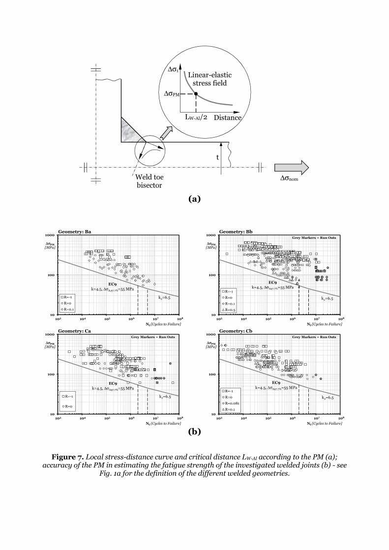
(a)

(b)

Figure 7. Local stress-distance curve and critical distance LW-Al according to the PM (a); accuracy of the PM in estimating the fatigue strength of the investigated welded joints (b) - see

Fig. 1a for the definition of the different welded geometries.

10

100

1000

1000 10000 100000 1000000 10000000 100000000

∆σPM

[MPa]

Nf [Cycles to Failure]

Geometry: Ba

R=-1

R=0

R=0.1

EC9

k=4.5, ∆σA,97.7%=55 MPa

103 104 105 106 107 108

k2=6.5

10

100

1000

1000 10000 100000 1000000 10000000 100000000

∆σPM

[MPa]

Nf [Cycles to Failure]

Geometry: Bb

R=-1

R=0

R=0.1

R=0.5

Grey Markers = Run Outs

EC9

k=4.5, ∆σA97.7%=55 MPa

103 104 105 106 107 108

k2=6.5

10

100

1000

1000 10000 100000 1000000 10000000 100000000

∆σPM

[MPa]

Nf [Cycles to Failure]

Geometry: Ca

R=-1

R=0

Grey Markers = Run Outs

EC9

k=4.5, ∆σA97.7%=55 MPa

103 104 105 106 107 108

k2=6.5

10

100

1000

1000 10000 100000 1000000 10000000 100000000

∆σPM

[MPa]

Nf [Cycles to Failure]

Geometry: Cb

R=-1

R=0

R=0.081

R=0.1

Grey Markers = Run Outs

EC9

k=4.5, ∆σA97.7%=55 MPa

103 104 105 106 107 108

k2=6.5

∆σnom

t

Weld toe bisector

Distance

∆σ1 Linear-elastic

stress field

∆σPM

LW-Al/2

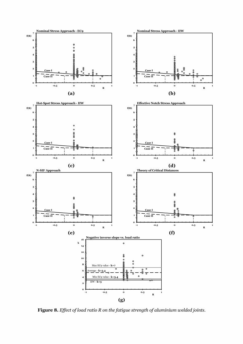
(a)

(b)

(c)

(d)

(e)

(f)

(g)

Figure 8. Effect of load ratio R on the fatigue strength of aluminium welded joints.

0

1

2

3

4

5

6

7

-1 -0.5 0 0.5 1

f(R)

R

Nominal Stress Approach - EC9

Case I

Case II

0

1

2

3

4

5

6

7

-1 -0.5 0 0.5 1

f(R)

R

Nominal Stress Approach - IIW

Case I

Case II

0

1

2

3

4

5

6

7

-1 -0.5 0 0.5 1

f(R)

R

Hot-Spot Stress Approach - IIW

Case I

Case II

0

1

2

3

4

5

6

7

-1 -0.5 0 0.5 1

f(R)

R

Effective Notch Stress Approach

Case I

Case II

0

1

2

3

4

5

6

7

-1 -0.5 0 0.5 1

f(R)

R

N-SIF Approach

Case I

Case II

0

1

2

3

4

5

6

7

-1 -0.5 0 0.5 1

f(R)

R

Theory of Critical Distances

Case I

Case II

0

2

4

6

8

10

12

14

16

-1 -0.5 0 0.5 1

k

R

Negative inverse slope vs. load ratio

Average - k=5.4

IIW - k=3

Max EC9 value - k=7

Min EC9 value - k=3.4

Figure A1. Wöhler diagram showing fatigue curves calculated for different probabilities of survival.

log Nf

log ∆σ

NA

∆σA.50%

∆σA,(1-P)%

∆σA,P%

1

1 1

k

k k

PS=50%

Log-Normal Distribution

PS=P%

PS=(1-P)%

Least-Squares Regression line