On Testing for Informative Selection in Survey Sampling 1

(plus Some Estimation)

Jay BreidtColorado State University

Survey Methods and their Use in Related FieldsNeuchatel, Switzerland

August 23, 2018

Joint work with various people, acknowledged as we go.

1

Goal: Inference for the distribution of Y 2

• Finite population U = {1, 2, . . . , N}• Random variables {Yk : k ∈ U} are independent and

identically distributed

• Observe the realized values not for all of U , but only arandom subset:

{yk : k ∈ s ⊂ U}

• Goal is inference on the distribution of Y , or some of itscharacteristics

• Concerned about effect of selection of s ⊂ U on inference

2

Sample membership indicators 3

• Define sample membership indicators Ik, where

Ik =

{1 if k ∈ s0 otherwise

• If the selection is designed/controlled, the event {k ∈ s}may depend on Yk

• If the selection is not designed/controlled, the event{k ∈ s} may depend on Yk

• Probability of selection, in general, may depend on Yk

3

Inclusion probabilities 4

• To allow probability of selection to depend on Yk, makeit random

• Inclusion probability is the realization of random variableΠk that may depend on Yk:

πk = P [Ik = 1 | Yk = yk,Πk = πk]

= E [Ik | Yk = yk,Πk = πk]

4

Examples with explicit dependence on Yk 5

• Cut-off sampling: πk = ρ(yk)1{yk>τ}.

• Case-control study (binary Y ):

πk =

{1, for disease cases (yk = 1)

ρ < 1, for non-disease controls (yk = 0)

• Choice-based sampling (categorical Y ):

πk =

J∑j=1

ρj1{yk=j}.

• Adaptive sampling, quota sampling, endogenousstratification, . . .

5

Length-biased sampling 6

• Length-biased sampling: πk ∝ yk > 0

• Good design for yk tries to be length-biased

•Why? For fixed size design,

Var

(∑k∈s

ykπk

∣∣∣∣∣Y U = yu,ΠU = πU

)= −1

2

∑j,k∈U

∆jk

(yjπj− ykπk

)2

= −1

2

∑j,k∈U

∆jk

(yjcyj− ykcyk

)2

= 0

• Unbiased estimator with zero variance!

6

Length-biased sampling: πk ∝ yk 7

y = textile fiber length (Cox, 1969), intercepted individual’s time

spent at recreational site, size of sighted wild animal, lifetime of marked-

recaptured individual, disease latency period,. . .

Sampling PointSampling Point

7

Implicit dependence on Yk 8

• Often, Πk does not depend explicitly on Yk, but Yk haspredictive power for Πk

• Consider parametric empirical models:

E [Πk | Yk = yk] = µ(yk; ξ),

where ξ are nuisance parameters with respect to Y

• Or consider nonparametric empirical models:

E [Πk | Yk = yk] = µ(yk),

8

The effect of selection 9

• Parametric model for average inclusion probability:

E [Πk | Yk = yk] = µ(yk; ξ)

• Relevant distribution of observed Yk is

f (y | Ik = 1) =µ(y; ξ)∫

µ(y; ξ)f (y) dyf (y) =: ρ(y; ξ)f (y),

in which the denominator depends on f

• If µ does not depend on y, then

f (y | Ik = 1) =µ(ξ)

µ(ξ)∫f (y) dy

f (y) = f (y)

9

Simple example 10

• Suppose Yk iid N (θ, σ2)

• Further suppose:

Πk | (Yk = yk) ∼ logN(ξ0 + ξyk, τ

2)

E [Πk | Yk = yk] = exp

(ξ0 + ξyk +

τ2

2

)• Then it is easy to show that

Yk | (Ik = 1) ∼ N(θ + ξσ2, σ2

),

so sample mean will be biased and inconsistent for θ

10

Application to a textbook survey 11

• Simulated data from Fuller (2009, Ex. 6.3.1) followingKorn and Graubard (1999, Ex. 4.3-1) for1988 National Maternal and Infant Health Survey

• Conducted by US National Center for Health Statistics

• Goal: study factors related to poor pregnancy outcome

• Design: nationally-representative stratified sample frombirth records, with oversampling of low-birthweightinfants

– complex survey: stratified, unequal-probability

11

Selection for NMIHS 12

• Let U = all US live births in 1988

• Let Yk = gestational age, strongly related to birthweight

• Suppose Yk iid N (θ, σ2)

• Inclusion probability in NMIHS depends on birthweight,hence Yk is predictive:

E [Πk | Yk = yk] = exp

(ξ0 − 0.175yk +

τ2

2

)• Greater gestational age ⇒ less likely to be sampled

12

Estimation for gestational age 13

• By previous computation, negative bias in the unweightedsample mean:

Yk | (Ik = 1) ∼ N(θ − 0.175σ2, σ2

),

> svymean(~GestAge, birth.design)

mean SE

GestAge 39.138 0.0941

> # Unweighted minus weighted:

> mean(birth$GestAge) - svymean(~GestAge, birth.design)

-2.2114

• Here we used classical design-based techniques to dealwith effects of selection

13

Horvitz-Thompson estimation 14

• Provided πk > 0 for all k ∈ U plus additional mildconditions,

θHT =1

N

∑k∈U

ykIkπk

is unbiased and consistent for finite-population average:

E

[1

N

∑k∈U

ykIkπk

∣∣∣∣∣ πU ,yU]

=1

N

∑k∈U

yk = θN

• Consistency for θ then follows by chaining argument:

θHT − θ =(θHT − θN

)+ (θN − θ) = small + smaller

14

Horvitz-Thompson plug-in principle: explicit 15

• If finite population parameter can be written explicitly as

θN = ϑ

∑k∈U

y(1)k , . . . ,

∑k∈U

y(p)k

for some smooth map ϑ(·), then

θHT = ϑ

∑k∈U

y(1)k

Ikπk, . . . ,

∑k∈U

y(p)k

Ikπk

is consistent and asymptotically design-unbiased for θN

15

Horvitz-Thompson plug-in principle: implicit 16

• If a finite population parameter can be written as solutionto a population-level estimating equation,

θN solves 0 = ϕ

∑k∈U

y(1)k , . . . ,

∑k∈U

y(p)k ; θ

,

then HT plug-in estimator is obtained by solving weightedsample-level estimating equation:

θHT solves 0 = ϕ

∑k∈U

y(1)k

Ikπk, . . . ,

∑k∈U

y(p)k

Ikπk

; θ

16

Pseudo-likelihood estimation 17

• If estimating equation uses the population-level score,

0 =∂

∂θ

∑k∈U

ln f (yk; θ)

∣∣∣∣∣θ=θN

,

then θN are population-level MLE’s

• If it uses the weighted sample-level score,

0 =∂

∂θ

∑k∈U

ln f (yk; θ)Ikπk

∣∣∣∣∣θ=θHT

,

then θHT are maximum pseudo-likelihood estimators

17

HT plug-in principle plus chaining argument 18

• Combining plug-in and chaining argument:

– Link 1: for the superpopulation model parameter θ,define a corresponding finite population parameter θN

– Link 2: estimate θN by θHT using HT plug-in principle

• Typically,

θHT−θ =(θHT − θN

)+(θN − θ) = Op

(n−α

)+Op

(N−α

)where n << N , so ignore the second component

• Use design-based methods to estimate the variance of thefirst component, ignoring the second

18

Options for dealing with selection 19

•Default Option: Assume informative selection

– use HT plug-in and chaining

– simple and readily available in software

– design-based option is not usually the most efficient

•Other Options: Test for informative selection

– if no evidence of selection effects, proceed with fully-efficient likelihood-based methods

– if evidence of selection effects, proceed with likelihood-based procedures that account for effects of selection

19

Likelihood-based approaches to estimation 20

•Pseudo-likelihood: easy but least efficient

• Full likelihood: most efficient, often impractical

– in general, joint distribution of all observed Yk, Ik,Πk– with no selection, joint distribution of Yk only

• Sample likelihood: treat {Yk}k∈s as if they wereindependently distributed with marginal pdf

f (y | Ik = 1) =µ(y; ξ)∫

µ(y; ξ)f (y) dyf (y)

• The typical efficiency ordering:

Pseudo < Sample < Full

20

Sample likelihood estimation 21

• Sample likelihood has long history:

– Patil and Rao (1978), Breslow and Cain (1988), Kriegerand Pfeffermann (1992), Pf., Krieger and Rinott (1998),Pf. and Sverchkov (2009)

• But theoretical foundation has been less developed:

– assuming n fixed as N →∞, PKR (1998) show point-wise convergence of joint pdf of responses to productof f (yk | Ik = 1)

•Want theoretical results that account for dependence in-duced by design

21

Our contribution to sample likelihood estimation 22

• Bonnery, Breidt, Coquet (2018, Bernoulli):

– assume√n-consistent and asymptotically normal se-

quence of estimators of nuisance parameters ξ

– often attainable via design-based regression: ξHT

– plug in ξHT to product of f (yk | Ik = 1; θ):∏k∈s

µ(yk; ξHT)∫µ(y; ξHT)f (y; θ) dy

f (yk; θ)

– maximize with respect to θ to get θSMLE

22

Our contribution to sample likelihood estimation, II 23

• Consistency and asymptotic normality of θSMLE

– assumptions are verifiable for some realistic designs

– asymptotic approximations work well in simulations

• Asymptotic covariance matrix depends on

– joint covariance matrix of score vector and ξHT, esti-mated via design-based methods

– information matrix for θ, estimated via model-basedmethods (plug SMLEs into analytic derivation)

• Design-based regression problem followed by classical like-lihood problem

23

Approaches to testing 24

•Approach 1: Test for dependence on yk of

E [Πk | Yk = yk] = µ(yk; ξ)

– this is a regression specification test

– parametric or nonparametric

•Approach 2: Test for a difference between design-weighted and unweighted . . .

– . . . parameter estimates

– . . . probability density function estimates

– . . . cumulative distribution function estimates

24

Intuition of Approach 2 25

• Design-weighted corrects for ρ and targets f (perhapsinefficiently)

• Unweighted does not correct for ρ and targets ρf

• Difference between weighted and unweighted indicatesρ 6≡ 1, so selection is informative

25

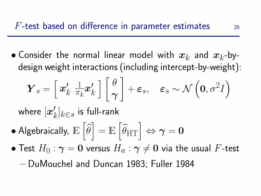
F -test based on difference in parameter estimates 26

• Consider the normal linear model with xk and xk-by-design weight interactions (including intercept-by-weight):

Y s =[x′k

1πkx′k

] [ θγ

]+ εs, εs ∼ N

(0, σ2I

)where [x′k]k∈s is full-rank

• Algebraically, E[θ]

= E[θHT

]⇔ γ = 0

• Test H0 : γ = 0 versus Ha : γ 6= 0 via the usual F -test

– DuMouchel and Duncan 1983; Fuller 1984

26

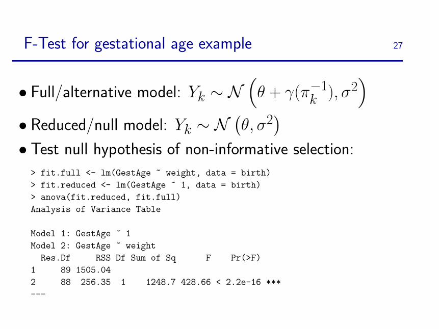
F-Test for gestational age example 27

• Full/alternative model: Yk ∼ N(θ + γ(π−1

k ), σ2)

• Reduced/null model: Yk ∼ N(θ, σ2

)• Test null hypothesis of non-informative selection:

> fit.full <- lm(GestAge ~ weight, data = birth)

> fit.reduced <- lm(GestAge ~ 1, data = birth)

> anova(fit.reduced, fit.full)

Analysis of Variance Table

Model 1: GestAge ~ 1

Model 2: GestAge ~ weight

Res.Df RSS Df Sum of Sq F Pr(>F)

1 89 1505.04

2 88 256.35 1 1248.7 428.66 < 2.2e-16 ***

---

27

Wald test based on difference in parameter estimates 28

•More generally, Pfeffermann (1993) derived the Wald-type test statistic,

WN =(θHT − θ

)′{−J−1 + J−1HTKHTJ

−1HT

}−1 (θHT − θ

)where J and K matrices depend on

π−1k , Var

(∂ log f (yk | θ)

∂θ

),∂2 log f (yk | θ)

∂θ ∂θ′

• Under the null hypothesis E[θHT − θ

]= 0, WN con-

verges in distribution to a chi-squared distribution withdegrees of freedom equal to dim(θ)

28

Test based on likelihood ratio 29

•Wald test requires considerable derivation

• Alternative test does not compare parameter estimatesdirectly, but evaluates their likelihood ratio

– unweighted log-likelihood ratio:

LR = 2{

lnL(θ)− lnL(θHT)}

– weighted (pseudo) log-likelihood ratio:

LRHT = 2{

lnLHT(θHT)− lnLHT(θ)}

• (W. Herndon, 2014 CSU dissertation advised by Breidt and Opsomer,

and joint with R. Cao and M. Francisco-Fernandez)

29

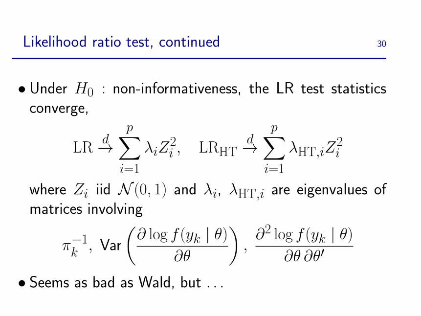
Likelihood ratio test, continued 30

• Under H0 : non-informativeness, the LR test statisticsconverge,

LRd→

p∑i=1

λiZ2i , LRHT

d→p∑i=1

λHT,iZ2i

where Zi iid N (0, 1) and λi, λHT,i are eigenvalues ofmatrices involving

π−1k , Var

(∂ log f (yk | θ)

∂θ

),∂2 log f (yk | θ)

∂θ ∂θ′

• Seems as bad as Wald, but . . .

30

Bootstrapping is easy 31

• Parametric bootstrap version of LR test statistic:

– draw bootstrap sample from fitted density and con-struct LR test statistic B times

– bootstrap p-value= B−1∑Bb=1 1{LR(b) > LR}

– simple to implement: no information computations

• Both the linear combination of χ21’s and the bootstrap

version work well in simulations

– correct size under H0

– good power for a range of informative designs

31

Now consider nonparametric estimation and tests 32

• Nonparametric density estimation and testing

– alternatives to “classic” design-weighted KDE

– compare design-weighted KDE to unweighted KDE fortesting?

• Nonparametric CDF estimation and testing

– brief review of CDF estimation under informative se-lection

– tests comparing design-weighted empirical CDF to un-weighted CDF

32

Kernel density estimation under informative selection 33

• Bonnery, Breidt, Coquet (2017, Metron)

• Under standard assumptions, unweighted KDE

1

n

∑k∈s

1

hK

(yk − yh

)with kernel K, bandwidth h converges not to f (y), but

µ(y; ξ)∫µ(y; ξ)f (y) dy

f (y) = ρ(y; ξ)f (y)

– usual O(h2) rate for bias, in estimation of ρf

– “usual” O((Nh

∫µf )−1

)variance

33

KDE under informative selection, continued 34

• Unweighted KDE converges to

µ(y; ξ)∫µ(y; ξ)f (y) dy

f (y) = ρ(y; ξ)f (y)

• “Outer adjustment”: use unweighted KDE

– estimate and remove ρ

– or estimate and remove µ and∫µf

• “Inner adjustment”: use weighted KDE

– weights from inclusion probabilities regressed on y

– or from design weights regressed on y

34

Outer = Inner for design-weighted KDE 35

• “Outer adjustment”: Estimating µ and∫µf via

design-weighted nonparametric regression leads to

1∑k∈s π

−1k

∑k∈s

1

hK

(yk − yh

)1

πk

• But this is just “Inner adjustment” using the originaldesign weights

• This standard, design-weighted KDE is the baseline forcomparison

35

Integrated MSE results with gestational age model 36

• n = 90, 1000 reps with 5-per-stratum in 18 strata

E [Π | Y = y] IMSE E[Π−1 | Y = y

]IMSE

= µ(y; ξ) Ratio = ω(y; δ) Ratio

µ, ξ known 1.5 — —Outer ξ unknown 1.7 — —

misspecified µ 1.6 misspecified ω 1.6kernel reg. 1.0 kernel reg. 0.96µ, ξ known 0.9 — —

Inner ξ unknown 0.96 — —misspecified µ 0.94 misspecified ω 0.93

kernel reg. 1.4 kernel reg. 1.4

36

Testing for informativeness using KDE? 37

• KDE summary:

– nonparametric outer adjustment works well

– parametric inner adjustment works slightly better

• Design-weighted or adjusted KDE converges to f

• Unweighted KDE converges to ρf

• At a minimum, this is an exploratory tool that may sug-gest informativeness

• Formal testing is a subject of future work

37

CDF estimation under informative selection 38

• Bonnery, Breidt, Coquet (2012, Bernoulli)

• Under mild conditions, the (unweighted) empirical CDF

F (α) =

∑k∈U 1(−∞,α](Yk)Ik

1 (IU = 0) +∑

k∈U Ik

converges uniformly in L2:

supα∈R

∣∣∣F (α)− Fρ(α)∣∣∣ = ‖F − Fρ‖∞

L2→N→∞

0

where the limit CDF is distorted by selection:

Fρ(α) =

∫ α−∞ µ(y; ξ)f (y) dy∫µ(y; ξ)f (y) dy

=

∫ α

−∞ρ(y; ξ)f (y) dy

38

Return to gestational age example 39

• Looks like informative selection: can we test?

25 30 35 40

0.0

0.2

0.4

0.6

0.8

1.0

Unweighted and Weighted CDF's

Gestational Age (weeks)

f(x)

●● ● ●● ●● ● ●●●●●● ●● ● ●●●● ●●● ●●●●●

●●●

●●●●●●

●

●

●

●●●

●

●●

●●

●

●●●●●●

●●●●

●●

●● ● ●●●● ● ●●●

●●●●●

●● ●●●●● ●●● ●

●●●●●●●

●●● ●●●●●●●

●●●●●●●●●●●●●●●●●●●●●●

●●●●

●●●●●●●

●●●●●●●●●●

● ●●

39

Classical tests based on empirical CDFs 40

• Functional CLT for independent empirical CDFs:

Dn(α) =

√n

2

{F

(1)n (α)− F (2)

n (α)}

converges in distribution to a Brownian bridge: zero-mean Gaussian process GF with covariance function

E [GF (s)GF (t)] = F (s ∧ t)− F (s)F (t)

• Kolmogorov–Smirnov two-sample test: ‖Dn(α)‖∞• Cramer–von Mises two-sample test:

∫∞−∞D2

n(α) dFn(α),

with Fn = ψF(1)n + (1− ψ)F

(2)n for some ψ ∈ [0, 1]

40

Adapting to the survey context 41

• Boistard, Lopuhaa, and Ruiz-Gazen (2017) develop func-tional CLT for

√n

{∑k∈U 1(Yk ≤ α)Ikπ

−1k

N− F (α)

}via assumptions on

– CLT for HT, to get finite dimensional distributions

– higher-order inclusion probabilities, to get tightness

• Adapt and extend to weighted minus unweighted CDF:

TN(α) =√n

{∑k∈U 1(Yk ≤ α)Ikπ

−1k

NHT

−∑

k∈U 1(Yk ≤ α)Ikn

}(Teng Liu, CSU PhD, 2019)

41

Adapting to the survey context, II 42

•Result: Under the null of no informative selection, TN(α)converges in distribution to a scaled Brownian bridge:zero-mean Gaussian process GF with covariance function

E [GF (s)GF (t)] = C {F (s ∧ t)− F (s)F (t)}where

C = limN→∞

n

N2

∑k∈U

E

[1

Πk

(1− NΠk

n

)2]

42

Adapting to the survey context, III 43

• Estimate the scaling factor

C = limN→∞

n

N2

∑k∈U

E

[1

Πk

(1− NΠk

n

)2]

using design-based methods:

CHT =n

N2HT

∑k∈U

Ikπ2k

(1− NHTπk

n

)2

43

Adapting to the survey context, IV 44

• Under probability-proportional-to-size sampling, the scalefactor simplifies further: with wk = π−1

k ,

Cpps = (Sw/w)2 (n− 1)/n ' (CVw)2

• Kolmogorov–Smirnov test of informative selection:

C−1/2‖Tn(α)‖∞• Cramer–von Mises test of informative selection:

C−1∫ ∞−∞

T 2n(α) dH(α),

with H = ψFHT + (1− ψ)F for some ψ ∈ [0, 1]

44

Test statistic distributions for gestational age 45

• Asymptotic distribution and empirical distribution of K–Sand C–vM, with n = 300 and 1000 reps

0.0 0.5 1.0 1.5 2.0

0.0

0.2

0.4

0.6

0.8

1.0

Kolmogorov−Smirnov Statistic

CD

F o

f K−

S S

tatis

tic

0.0 0.2 0.4 0.6 0.8 1.0

0.0

0.2

0.4

0.6

0.8

1.0

Cramer−von Mises Statistic

CD

F o

f C−

vM S

tatis

tic

45

Power for gestational age simulation 46

• Empirical ξ = 0.175 in Yk | (Ik = 1) ∼ N(θ − ξσ2, σ2

)• Choose grid of ξ ∈ [0, 0.03]; use n = 300 and 1000 reps each

0.000 0.005 0.010 0.015 0.020 0.025 0.030

0.0

0.2

0.4

0.6

0.8

1.0

ξ

Pow

er

KSCVMFCVMGCVMADD

46

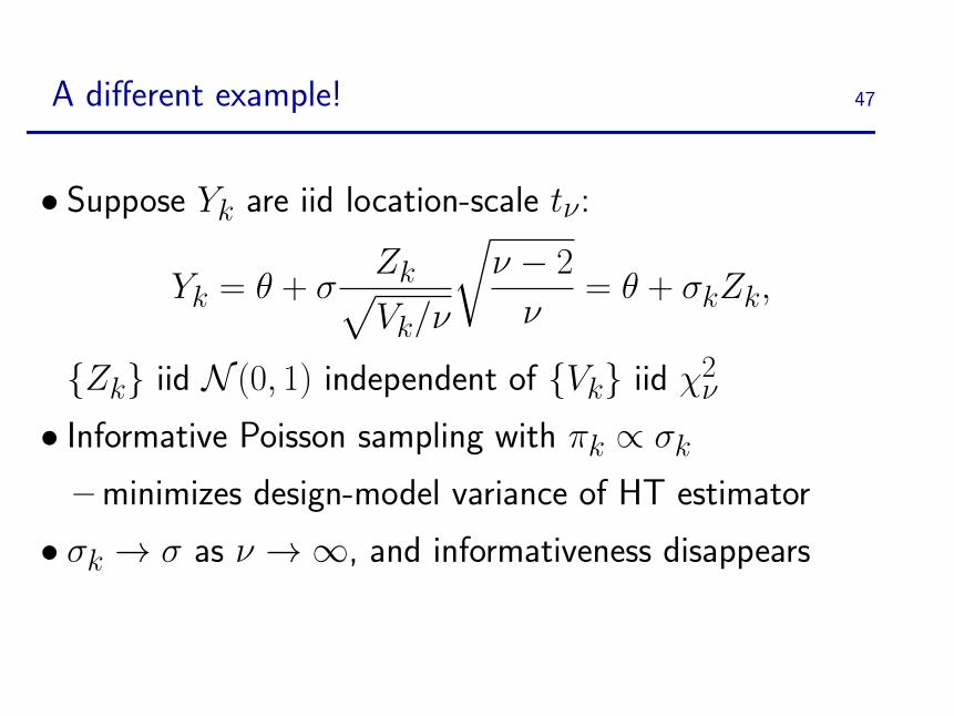
A different example! 47

• Suppose Yk are iid location-scale tν:

Yk = θ + σZk√Vk/ν

√ν − 2

ν= θ + σkZk,

{Zk} iid N (0, 1) independent of {Vk} iid χ2ν

• Informative Poisson sampling with πk ∝ σk

– minimizes design-model variance of HT estimator

• σk → σ as ν →∞, and informativeness disappears

47

Test statistic distributions for location-scale tν 48

• Asymptotic distribution and empirical distribution of K–Sand C–vM, with n = 300 and 1000 reps

0.0 0.5 1.0 1.5 2.0

0.0

0.2

0.4

0.6

0.8

1.0

Kolmogorov−Smirnov Statistic

CD

F o

f K−

S S

tatis

tic

0.0 0.2 0.4 0.6 0.8 1.0

0.0

0.2

0.4

0.6

0.8

1.0

Cramer−von Mises Statistic

CD

F o

f C−

vM S

tatis

tic

48

Power for location-scale tν simulation 49

• Choose ν = 22, 23, . . . , 29; use n = 300 and 1000 reps each

• DD test gets some “lucky” power at low df due to random variation

9 8 7 6 5 4 3 2

0.0

0.2

0.4

0.6

0.8

1.0

log2(ν)

Pow

er

KSCVMFCVMGCVMADD

49

Lucky power? 50

•Weighted and unweighted estimators have the same mean

• At very low degrees of freedom, HT is (particularly) highlyvariable

• Difference between weighted and unweighted is large dueto chance variation

• DD correctly rejects by incorrectly assuming largedifference is a difference in the mean

50

Summary 51

• Informative selection is pervasive

• Strategy of comparing weighted to unweighted works broadly:

– parametric, from linear models to likelihood ratios

– nonparametric, from kernel density estimation toclassic two-sample tests

• Design-weighted estimation is a “safe” and readily-availablesolution

• Sample likelihood approach is a viable alternative

51

THANK YOU 52

• Thank you for your attention

• Thanks to Matthieu, Guillaume, and Yves for a wonderfulconference!

52