On some information geometric approaches tocyber security

CTJ Dodson

School of Mathematics, University of Manchester, Manchester M13 9PL, UKctdodson@manchester.ac.uk

Abstract. Various contexts of relevance to cyber security involve theanalysis of data that has a statistical character and in some cases theextraction of particular features from datasets of fitted distributions orempirical frequency distributions. Such statistics, for example, may becollected in the automated monitoring of IP-related data during access-ing or attempted accessing of web-based resources, or may be triggeredthrough an alert for suspected cyber attacks. Information geometry pro-vides a Riemannian geometric framework in which to study smoothlyparametrized families of probability density functions, thereby allowingthe use of geometric tools to study statistical features of processes andpossibly the representation of features that are associated with attacks.In particular, we can obtain mutual distances among members of thefamily from a collection of datasets, allowing for example measures ofdepartures from Poisson random or uniformity, and discrimination be-tween nearby distributions. Moreover, this allows the representation oflarge numbers of datasets in a way that respects any topological featuresin the frequency data and reveals subgroupings in the datasets usingdimensionality reduction. Here some results are reported on statisticaland information geometric studies concerning pseudorandom sequences,encryption-decryption timing analyses, comparisons of nearby signal dis-tributions and departure from uniformity for evaluating obscuring tech-niques.

Keywords: cyber security, empirical frequency distributions, pseudo-random sequences, encryption-decryption timing, proximity to unifor-mity, nearby signals discrimination, information geometry, gamma dis-tributions, Gaussian distributions, dimensionality reduction

1 Introduction

The British Columbia Institute of Technology (BCIT) maintains an industrialcyber security incident database (ISID) [7], designed to track incidents of a cy-ber security nature that directly affect industrial control systems and processes.Byres and Lowe [8,7] pointed out that from 1980 to 2000 the cyber threat wasevenly split among internal, external and accidental cases. By 2001 this hadchanged to 70% external threat sources, 20% accidental, 5% internal and 5%other. Of these the internal security incidents arose from the following entry

points: business network 43%, human machine interface (HMI) 29%, physicalaccess to equipment 21% and laptop 7%. Externally the percentages includedattacks from: remote internet 36%, remote dial-up 20%, remote unknown 12%,VPN connection 8%, remote wireless 8%, the remainder from remote trustedthird party, remote Telco network, remote supervisory control and data acqui-sition (SCADA) network. The consequences of these attacks was a productionloss of 41% and loss of ability to control or view the plant. Between 1995 and2000 the number of security incidents averaged 2 per year but that had increasedlinearly to 10 per year by 2003. The UK government Centre for the Protectionof National Infrastructure (CPNI) [18] and the USA Homeland Security [35]provide up to date information and advice on cyber security.

In this paper we offer some geometrical methods for application in problemsof cyber security which can be addressed through statistical analyses of data.Information geometry provides a Riemannian geometric framework in which tostudy smoothly parametrized families of probability density functions, therebyallowing the use of geometric tools to study statistical features of processes. Ge-ometrical provision of this kind has proved an enormous advantage in theoreticalphysics and conversely, physical problems have stimulated many advances in dif-ferential geometry, global analysis and algebraic geometry. The geometrizationof statistical theory [1,2,3,4,5,21] has had similar success and its role in applica-tions is now widespread and generating new developments of theory, algorithmsand computational information geometry [46,47]. We give a brief introductionto information geometry in §2 and §2.1, which is sufficient for the understandingof techniques in the sequel. We outline the information geometry of univariateand multivariate Gaussians in §2.2, which we use in §7. Situations in which suchmethods are relevant to cyber security include discrimination between nearbysignal distributions, comparisons of real signal distributions with those obtainedvia random number generators in testing obscuring procedures, and in testingfor anomalous behaviour, for example using departures from uniformity or inde-pendence.

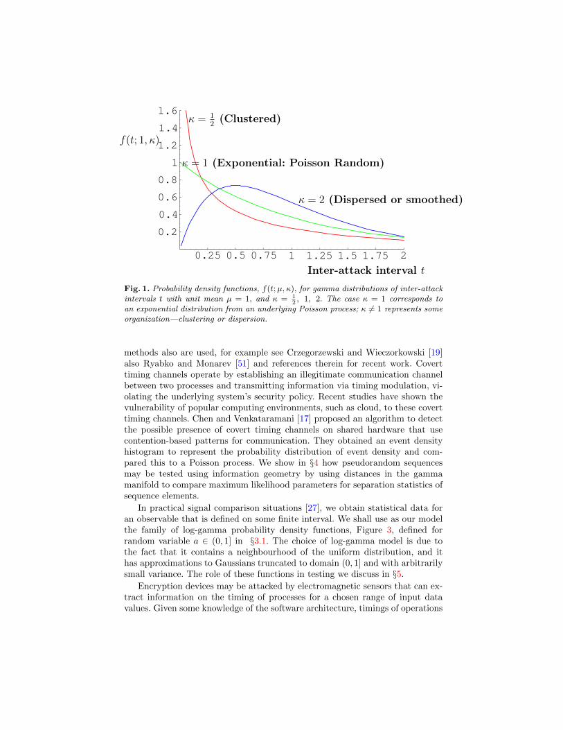
One aspect of cyber security is concerned with the analysis of the stochas-tic process of attack events [20]. Such analyses can yield valuable data on thefrequency distributions of attacks and these may be amenable to study usinginformation geometric methods. In particular, spacings between events of inter-est may be representable via gamma distributions, since they span a range ofbehaviour from clustered through random (ie Poisson) to dispersed, Figure 1; wediscuss their information geometry in §3. Gamma distributions have the prop-erty that the standard deviation is proportional to the mean, characterized inTheorem 1 below, and they include a representation of Poisson processes throughthe 1-parameter family of exponential distributions; this is represented in Fig-ure 2. Their information geometry was used in a variety of applications [5,23].In a range of contexts in cryptology for encoding, decoding or for obscuringprocedures, sequences of pseudorandom numbers are generated. Tests for ran-domness of such sequences have been studied extensively and the NIST Suite oftests [50] for cryptological purposes is widely employed. Information theoretic

0.25 0.5 0.75 1 1.25 1.5 1.75 2

0.2

0.4

0.6

0.8

1

1.2

1.4

1.6

f(t; 1, κ)

κ = 12

(Clustered)

κ = 1 (Exponential: Poisson Random)

κ = 2 (Dispersed or smoothed)

Inter-attack interval t

Fig. 1. Probability density functions, f(t;µ, κ), for gamma distributions of inter-attackintervals t with unit mean µ = 1, and κ = 1

2, 1, 2. The case κ = 1 corresponds to

an exponential distribution from an underlying Poisson process; κ 6= 1 represents someorganization—clustering or dispersion.

methods also are used, for example see Crzegorzewski and Wieczorkowski [19]also Ryabko and Monarev [51] and references therein for recent work. Coverttiming channels operate by establishing an illegitimate communication channelbetween two processes and transmitting information via timing modulation, vi-olating the underlying system’s security policy. Recent studies have shown thevulnerability of popular computing environments, such as cloud, to these coverttiming channels. Chen and Venkataramani [17] proposed an algorithm to detectthe possible presence of covert timing channels on shared hardware that usecontention-based patterns for communication. They obtained an event densityhistogram to represent the probability distribution of event density and com-pared this to a Poisson process. We show in §4 how pseudorandom sequencesmay be tested using information geometry by using distances in the gammamanifold to compare maximum likelihood parameters for separation statistics ofsequence elements.

In practical signal comparison situations [27], we obtain statistical data foran observable that is defined on some finite interval. We shall use as our modelthe family of log-gamma probability density functions, Figure 3, defined forrandom variable a ∈ (0, 1] in §3.1. The choice of log-gamma model is due tothe fact that it contains a neighbourhood of the uniform distribution, and ithas approximations to Gaussians truncated to domain (0, 1] and with arbitrarilysmall variance. The role of these functions in testing we discuss in §5.

Encryption devices may be attacked by electromagnetic sensors that can ex-tract information on the timing of processes for a chosen range of input datavalues. Given some knowledge of the software architecture, timings of operations

typically relate to modular exponentiation steps, associated with the processingof the binary bits in the encryption key. This is discussed in §6. In practice, cluesto such timing information can be obtained from data on power consumptionusing electromagnetic sensors, possibly needing statistical processes to clean thedata of noise. Kocher et al [39] showed the effectiveness of Differential PowerAnalysis (DPA) in breaking encryption procedures using correlations betweenpower consumption and data bit values during processing, claiming that mostsmart cards revealed their DES keys using fewer than 15 power traces. A prac-ticable defence is to obscure the power usage data on timing information byspurious other processes. Then the effectiveness of such obscuring techniquescan be evaluated using analyses of the distributions associated with time seriesfrom power usage. For example, a time series of power consumption using appro-priately chosen threshholding and interval windows would yield a barchart andthat would ideally be like that arising from Poisson processes, which for a givenmean are maximally disorderd [34]. Information geometry can be used to mea-sure differences from the Poisson model, equivalently from its associated expo-nential distribution—note that Grzegorzewski and Wieczorkowski [19] provideda detailed analysis of their entropy-based goodness-of-fit test for exponentiality.

Evaluation of cyber security may involve also identifying potentially anoma-lous behaviour in internet traffic on a network [48], thus requiring extractionof appropriate features from a large data set of event frequency distributions.sometimes we can fit standard models to the empirical frequency distributionsusing maximum likelihood methods as iillustrated for gamma distributions in §3.In the absence of a model family of distributions for which we have expressionsfor the information distances among the memberrs, we can use the symmetrizedKullback-Leibler relative entropy expression, equation (42), to measure distancebetween empirical frequency distributions. Once we have extracted distance mea-sures between all pairs of datasets we can use multi-dimensional scaling, or di-mensionality reduction, to extract the three most significant features from thedata set so that all samples can be displayed graphically in a 3-dimensional plot.The aim is to reveal groupings of data points that correspond to the prominentcharacteristics, the methodology is discussed in §7.

Such a dimensionality reduction can reveal anomalous behaviour of a pro-cess by taking account of the true curved geometry of the data set, rather thandisplaying it as uncurved in a Euclidean geometry (cf. [11], Figure 3.2). Thesignificance is that any non-obvious global topology of frequency connectivity inthe data is revealed by the pattern of mutual separations in the embedding. Anillustration using router traffic on the Abilene network showed how anomalousbehaviour unseen by local methods could be picked up through dimensionalitychanges (cf. [11], Figure 3.10). Moreover, in document classification, the infor-mation metric approach outperformed standard Principal Component Analysisand Euclidean embeddings [12], and it outperformed traditional approaches tovideo indexing and retrieval with real world data [16]. In §7 we outline how au-tocovariance extraction from time series data may be studied using information

geometry and dimensionality reduction; we described an application to datasetsof stochastic textures from 2-dimensional pixel arrays in [26].

We begin here by outlining the method to compute the Fisher informationmetric on a smoothly parametrized family of probability density functions, thenillustrate it with explicit expressions for some important examples.

2 The Fisher information metric

Let Θ ⊆ Rn be the parameter space of an n-dimensional smooth family ofprobability density functions defined on some fixed d-dimensional event spaceΩ ⊆ Rd, so we have a set

pθ|θ ∈ Θ with pθ ≥ 0 and

∫Ω

pθ = 1 for all θ ∈ Θ.

A fundamental property of a probability density function pθ is its Shannon en-tropy, which is the negative of the expectation of its log-likelihood function,l = log pθ, namely:

S(pθ) = −∫Ω

pθ log(pθ). (1)

The derivatives of the log-likelihood function, l = log pθ, yield a matrix func-tion on Ω and the expectation of its entries is

gij =

∫Ω

pθ

(∂l

∂θi∂l

∂θj

)= −

∫Ω

pθ

(∂2l

∂θi∂θj

), (2)

for coordinates (θi) about θ ∈ Θ ⊆ Rn.This gives rise to a positive definite matrix depending only on the parame-

ters, inducing a Riemannian metric structure g as a positive-definite symmetricquadratic form, on the space Θ of parameters (θi). From the construction of(2), a smooth invertible transformation of random variables, that is of the la-belling of the points in the event space Ω while keeping the same parameters(θi), will leave the Riemannian metric unaltered. Formally, it induces a smoothdiffeomorphism of manifolds that preserves the metric. This is a Riemannianisometry and the diffeomorphism is simply the identity map on parameters [5].We shall see this explicitly below for the case of the log-gamma distribution §3.1and its associated Riemannian manifold.

The elements in the matrix (2) define the arc length function

ds2 =∑i,j

gij dθi dθj , often abbreviated to ds2 = gij dθ

i dθj (3)

using the convention to sum over repeated indices.The metric (2) is called the expected information metric or Fisher-Rao or

Fisher metric for the manifold obtained from the family of probability densityfunctions; the original ideas are due to Fisher [30] and C.R. Rao [49]. The second

equality in equation (2) depends on certain regularity conditions [52] but whenit holds it can be particularly convenient to use. Amari [1,2,3] and Amari andNagaoka [4], provide accounts of the differential geometry that arises from theinformation metric. A wide range of applications is studied in [5,23].

2.1 Exponential family of distributions

An n-dimensional parametric statistical model Θ ≡ pθ|θ ∈ Θ is said to be anexponential family or of exponential type, when the probability density functionsin the family can be expressed in terms of functions C,F1, ..., Fn on Ω and afunction ϕ on Θ as:

p(x; θ) = eC(x)+∑i θi Fi(x)−ϕ(θ) , (4)

then we say that (θi) are its natural parameters, and ϕ is the potential function.From the normalization condition

∫p(x; θ) dx = 1 we obtain:

ϕ(θ) = log

∫Ω

eC(x)+∑i θi Fi(x) dx . (5)

This potential function is therefore a distinguished function of the coordinates(θi) alone and use can be made of it for the presentation of the manifold as animmersion in Rn+1 as follows:

Φ : Rn → Rn+1 : (θi) = θ 7→ (θ, ϕ(θ)) . (6)

With ∂i = ∂∂θi , we use from §2 the log-likelihood function l(θ, x) = log(pθ(x))

to obtain

∂il(θ, x) = Fi(x)− ∂iϕ(θ)

and

∂i∂j l(θ, x) = −∂i∂jϕ(θ) .

The information metric g on the n-dimensional space of parameters Θ ⊂ Rn,equivalently on the set S = pθ|θ ∈ Θ ⊂ Rn, has coordinates:

[gij ] = −∫Ω

[∂i∂j l(θ, x)] pθ(x) dx = ∂i∂jϕ(θ) = ϕij(θ) . (7)

Then, (S, g) is a Riemannian n-manifold. Distances between points in this man-ifold are computed as the geodesic length between the points, which is the infi-mum over all curves joining the points and in general difficult to obtain analyt-ically [25,5].

2.2 Information geometry of Gaussians

The family of univariate normal or Gaussian density functions has event spaceΩ = R and probability density functions given by

N ≡ N(µ, σ2) = n(x;µ, σ)|µ ∈ R, σ ∈ R+ (8)

depending smoothly on the parameters mean µ and variance σ2. So topologically,N = R × R+ is the upper half–plane, and the random variable is x ∈ Ω = Rwith

n(x;µ, σ) =1√

2π σe−

(x−µ)2

2 σ2 (9)

The mean µ and standard deviation σ are commonly used as a local coordinatesystem (µ, σ). However, the univariate Gaussians (9) are of exponential typewith natural coordinates θ1 = µ

σ2 and θ2 = − 12σ2 . Then ( µσ2 ,− 1

2σ2 ) is a naturalcoordinate system and

ϕ = − θ12

4 θ2+

1

2log(− π

θ2) =

µ2

2σ2+ log(

√2π σ) (10)

is the corresponding potential function defined in §2.1.Multivariate Gaussians for a given k = 2, 3, . . . ..., N are parametrized by a k-

vector of means µ ∈ Rk and a symmetric k×k covariance matrix Σ ∈ R(k2+k)/2.There is no analytic expression for the information distance between two gen-eral k-variate Gaussians. What we have analytically are natural norms, on thespace of means and on the space of covariances, giving the information distanceD(fA, fB) between two k-Gaussians fA(µA, ΣA) and fB(µB , ΣB) in two par-ticular cases:

ΣA = ΣB = Σ : The common positive definite symmetric quadratic form Σgives a norm on the difference vector of means:

Dµ(fA, fB) =

√(µA − µB)

T ·Σ−1 · (µA − µB). (11)

µA = µB = µ : A positive definite symmetric matrix constructed from the twocovariance matrices ΣA and ΣB is

SAB = ΣA−1/2 ·ΣB ·ΣA−1/2, with λABj = Eig(SAB)

and it gives a norm on the space of differences between covariances [6] so wehave

DΣ(fA, fB) =

√√√√1

2

k∑j=1

log2(λABj ). (12)

In principle, (12) yields all of the true geodesic distances since the informationmetric is invariant under affine transformations of the mean [6] Appendix 1; seealso the article of P.S. Eriksen [28].

In practice, an approximate distance that is monotonically related to the trueinformation distance may serve the purpose at hand, for example the symmetricsum:

D(fA, fB) ≈ 1

2

(Dµ(fA, fB) +Dµ(fB , fA)

)+DΣ(fA, fB),

which adds to the value of (12) the average of (11) using both available covari-ances.

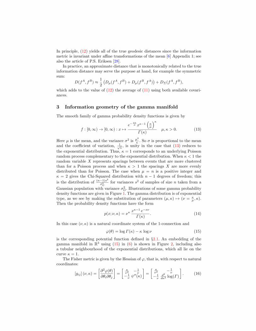
3 Information geometry of the gamma manifold

The smooth family of gamma probability density functions is given by

f : [0,∞)→ [0,∞) : x 7→e−

xκµ xκ−1

(κµ

)κΓ (κ)

µ, κ > 0. (13)

Here µ is the mean, and the variance σ2 is µ2

κ . So σ is proportional to the meanand the coefficient of variation, 1√

κ, is unity in the case that (13) reduces to

the exponential distribution. Thus, κ = 1 corresponds to an underlying Poissonrandom process complementary to the exponential distribution. When κ < 1 therandom variable X represents spacings between events that are more clusteredthan for a Poisson process and when κ > 1 the spacings X are more evenlydistributed than for Poisson. The case when µ = n is a positive integer andκ = 2 gives the Chi-Squared distribution with n − 1 degrees of freedom; this

is the distribution of (n−1)s2σ2G

for variances s2 of samples of size n taken from a

Gaussian population with variance σ2G. Illustrations of some gamma probability

density functions are given in Figure 1. The gamma distribution is of exponentialtype, as we see by making the substitution of parameters (µ, κ) 7→ (ν = κ

µ , κ).Then the probability density functions have the form

p(x; ν, κ) = νκxκ−1 e−xν

Γ (κ). (14)

In this case (ν, κ) is a natural coordinate system of the 1-connection and

ϕ(θ) = logΓ (κ)− κ log ν (15)

is the corresponding potential function defined in §2.1. An embedding of thegamma manifold in R3 using (15) in (6) is shown in Figure 2, including alsoa tubular neighbourhood of the exponential distributions, which all lie on thecurve κ = 1.

The Fisher metric is given by the Hessian of ϕ, that is, with respect to naturalcoordinates:

[gij ] (ν, κ) =

[∂2ϕ(θ)

∂θi∂θj

]=

[κν2 − 1

ν− 1ν ψ′′(κ)

]=

[ κν2 − 1

ν

− 1ν

d2

dκ2 log(Γ )

]. (16)

Fig. 2. An embedding of the gamma manifold in R3 using (15) in (6) including also atubular neighbourhood of the exponential distributions, which all lie on the curve κ = 1.

In terms of the original parameters (µ, κ) in (13) the metric turns out to bediagonal:

[gij ] (µ, κ) = =

[κµ2 0

0 d2

dκ2 log(Γ )− 1κ

]. (17)

So the coordinates (µ, κ) yield an orthogonal basis of tangent vectors, which isuseful in calculations because then the arc length function is simply

ds2 =κ

µ2dγ2 +

((Γ ′(κ)

Γ (κ)

)′− 1

κ

)dκ2.

We note the following important uniqueness property:

Theorem 1 (Cf [42,36,23]). For independent positive random variables witha common probability density function f, having independence of the samplemean and the sample coefficient of variation is equivalent to f being the gammadistribution.

A proof of Theorem 1 was given in [36] but in fact the result seems to havebeen known much earlier and in [23] we gave a proof partly based on the 1954article by Laha [42], of interest for the methodology using Laplace Transforms,which are related to moment generating functions in statistics [29]. Other usefulinformation geometric results involve very commonly occurring distributions andhave been applied in a number of areas [5,23]. Some may have application inmeasuring and representing statistical processes relevant to cyber security whenthere is a need to study the neighbourhood of a target distribution:

Theorem 2. Every neighbourhood of a Poisson process contains a neighbour-hood of processes subordinate to gamma probability density functions.

Theorem 3. Every neighbourhood of a uniform process contains a neighbour-hood of processes subordinate to log-gamma probability density functions.

Theorem 4. Every neighbourhood of an independent pair of identical Poissonprocesses contains a neighbourhood of bivariate processes subordinate to Freundbivariate exponential probability density functions.

Theorem 5. The 5-dimensional space of bivariate Gaussians admits a 2-dimensionalsubspace through which can be provided a neighbourhood of independence for bi-variate Gaussian processes.

Theorem 6. Via the Central Limit Theorem, by continuity, the tubular neigh-bourhoods of the curve of zero covariance for bivariate Gaussian processes willcontain all limiting bivariate processes sufficiently close to the independence casefor all processes with marginals that converge in probability density function toGaussians.

The characterizing property in Theorem 1 is one of the main reasons forthe large number of applications of gamma distributions: many families of near-random natural processes have standard deviation approximately proportionalto the mean [5], increasing together with time or changing ambient conditions,and this is easily tested for in practice. To fit a gamma distribution to data wecan obtain the maximum likelihood parameter values µ, κ, as follows.

Given a set of identically distributed, independent data valuesX1, X2, . . . , Xn,the ‘maximum likelihood’ or ‘maximum entropy’ parameter values µ, κ for fit-ting the gamma distribution (13) are computed in terms of the mean and meanlogarithm of the Xi by maximizing the likelihood function

Lf (µ, κ) =

n∏i=1

f(Xi;µ, κ).

By taking the logarithm and setting the gradient to zero we obtain

µ = X =1

n

n∑i=1

Xi (18)

log κ− Γ ′(κ)

Γ (κ)= log X − 1

n

n∑i=1

logXi

= log X − logX. (19)

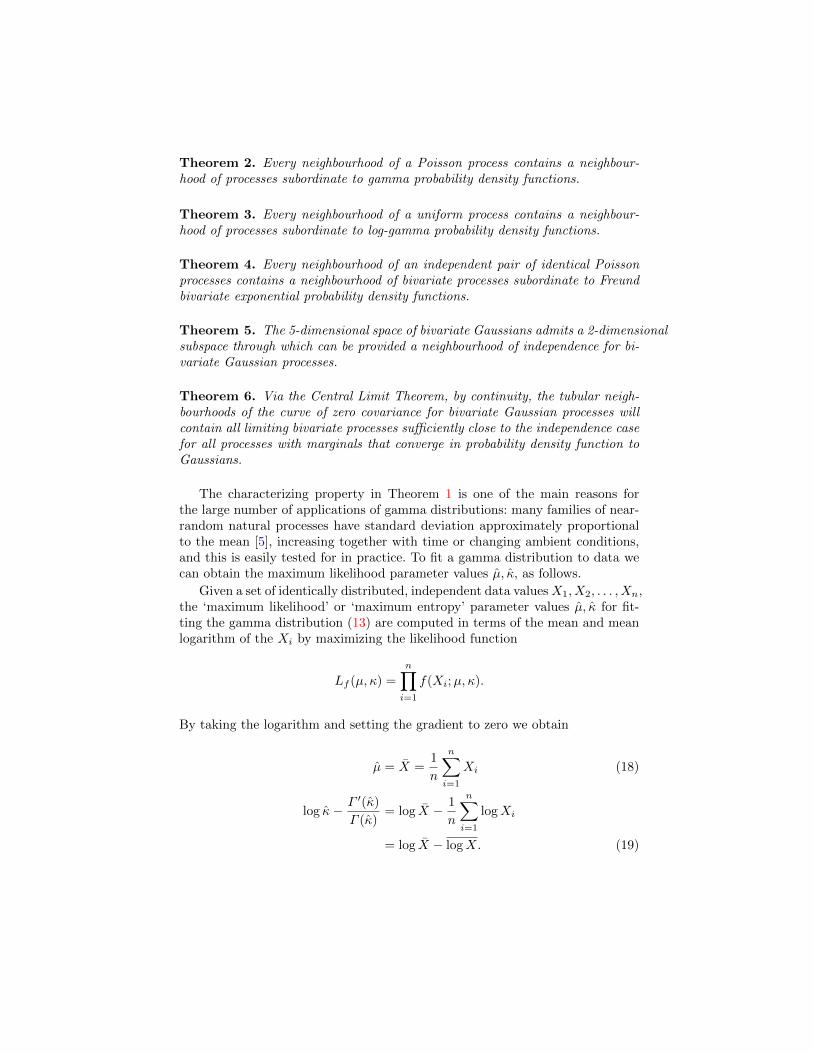
Fig. 3. The log-gamma family of probability densities (21) with central mean a = 12

asa surface. The surface tends to the delta function as κ → ∞ and coincides with theconstant 1 at κ = 1.

3.1 Neighbourhoods of uniformity in the log-gamma manifold

The log-gamma density (21) actually arises from the gamma density

f(x, µ, κ) =xκ−1 µκ

Γ (κ)e−xµ. (20)

via the change of variable from x ∈ R+ to a ∈ (0, 1] via x = − log a.The smooth family of log-gamma distributions has probability density func-

tions of form

P (a, µ, κ) =aµ−1µκ

∣∣log(1a

)∣∣κ−1Γ (κ)

(21)

for random variable a ∈ (0, 1] and parameters µ, κ > 0, see Figure 10. The meanand variance are given by

a = E(a) =

(µ

1 + µ

)κ(22)

σ2(a) =

(µ

µ+ 2

)κ−(

µ

1 + µ

)2κ

. (23)

In this family the locus of those with central mean E(a) = 12 satisfies

µ(21κ − 1) = 1 (24)

shown in Figure 3; the uniform density is the special case with κ = µ = 1.Figure 4 shows a spherical neighbourhood in Euclidean space centred on the

Fig. 4. An affine immersion in Euclidean space R3 of the curved surface of log-gammaprobability densities on (0, 1]. The two curves in the surface represent the log-gammadistributions with ν = 1 and κ = 1, and the spherical neighbourhood in R3 is centredon their intersection, which point represents the uniform distribution.

point at the uniform density on (0, 1] in the curved surface representing all log-gamma distributions; the uniform density is represented by the point ν = 1, κ =1. This provides a method to measure departures from uniformity. The impor-tant information geometric property is that the Riemannian manifold of gammadistributions is isometric to that of log-gamma distributions, this is discussedwith applications in [5].

3.2 Neighbourhoods of randomness in the gamma manifold

Cyber software sometimes uses pseudorandom number generators to provide seednumbers for algorithms and sequences for testing procedures or for comparisonwith application sequences in attempts to obscure internal processes, which oth-erwise might reveal clues to the timing of underlying operations through powertraces. Cryptological attacks on encryption/decryption devices may be defendedagainst by obscuring algorithms that overlay randomizing procedures; then thereis a need to compare nearby signal distributions and again the information metriccan help. The Poisson distribution of events on a line is such that the proba-bility of an event in an interval depends only on the size of the interval, noton the position of the interval in the line. Then the distribution of lengths of

intervals between successive events is easily shown to be exponential, and thatdistribution has maximal entropy within the family of gamma distributions, soit is maximally haphazard and involves fewest assumptions.

Tests for randomness of number sequences have been studied extensivelyand the NIST Suite of tests [50] for cryptological purposes is widely employed.Information theoretic methods also are used, for example see [19] also [51] andreferences therein for recent work. In [23] we added to the latter by outlining howfinite length pseudorandom sequences may be tested quickly and easily using in-formation geometry by computing distances in the gamma manifold to comparemaximum likelihood parameters for separation statistics of sequence elements.A Poisson process defines a unique exponential distribution, the exponential dis-tributions with different means are special cases of gamma distributions and theinformation geometry of the gamma family determines a metric structure forneighbourhoods, cf. Figure 2, of the 1-parameter curve of exponential distribu-tions in the Riemannian manifold of gamma distributions [5].

0 100 200 300 400 500

0.8

1.0

1.2

1.4

1.6κ

Fig. 5. The problem of finite length pseudorandom sequences. Maximum likelihoodgamma parameter κ fitted to separation statistics for simulations of Poisson line pro-cesses of length 100000 with expected parameter κ = 1. These simulations used thepseudorandom number generator in Mathematica [54]. In the limit, as the sequencelength tends to infinity we expect the gamma parameter µ to tend to 1.

Mathematica [54] simulations were made of Poisson line processes using ran-dom number sequences of length n = 100000 for which spacing statistics werecomputed [23]. Figure 5 shows maximum likelihood gamma parameter κ valuesfrom the simulations. The surface height in Figure 6 represents upper bounds oninformation geometric distances from (µ, κ) = (511, 1) in the gamma manifold.This employs the approximate geodesic mesh function we described in Arwini

and Dodson [5].

Distance[(511, 1), (µ, κ)] ≤∣∣∣∣d2 logΓ

dκ2(κ)− d2 logΓ

dκ2(1)

∣∣∣∣+

∣∣∣∣log511

µ

∣∣∣∣ . (25)

The points shown in Figure 6 are maximum likelihood gamma parameters fromthe Mathematica simulations of Poisson random processes of 100000 events withexpected separation µ = 511. In the data from 500 such simulations the rangesof maximum likelihood gamma parameters were

419 ≤ µ ≤ 643 and 0.62 ≤ κ ≤ 1.56.

So, even with strings of 100, 000 nominally random numbers, there is consider-

Surface of distance from (µ, κ) = (511, 1)

Fig. 6. Distances in the space of gamma models, using a geodesic mesh. The surfaceheight represents upper bounds on distances from the target (µ, κ) = (511, 1) fromEquation (25). Also shown are data points of maximum likelihood gamma parametersfor interval lengths between events from simulations of Poisson random processes of100000, for events with expected separation µ = 511. In the limit as the sequence lengthtends to infinity we expect the gamma parameter κ to tend to 1.

able variability from the expected distribution of spacings in the sorted strings.Clearly as the sequence length tends to infinity we expect the gamma parame-ter κ to tend to 1. However, finite sequences must be used in real applicationsand then provision of a metric structure allows us, for example, to comparereal sequence generating procedures against an ideal Poisson random model inthe space of gamma distributions. Representations like that in Figure 6 couldbe used to trigger an alert or action when an automated updating sequence ofevents abnormally strays over a chosen threshold of distance from a target.

4 Statistics of finite random spacing sequences

In the perfectly random case of haphazard allocation of events along a time line,the result is an exponential distribution of inter-event intervals when the line isinfinite. However, for finite length processes it is a little more involved and weneed to analyse this first in order to provide our reference structure.

Think of a sequence of different events among which we have distinguishedone, represented by the letter X, while all others are represented by ?. In thecyber security context, X is the event of an attack. The relative abundance of Xis given by the probability p that an arbitrarily chosen location in the sequencehas an occurrence of X. Then 1−p is the probability that the location contains adifferent event from X. If the locations of X are chosen with uniform probabilitysubject to the constraint that the net density of X in the chain is p, then eitherX happens or it does not; we have a binomial process.

It follows that, in a sequence of n events, the mean or expected number ofoccurrences of X is np and its variance is np(1 − p), but it is not immediatelyclear what will be the distribution of lengths of intervals between consecutiveoccurrencies of X. Evidently the distribution of such lengths r, measured in unitsof one location length also is controlled by the underlying binomial distribution.

We are interested in the probability of finding in a sequence of n events asubsequence of form

· · ·?X︷ ︸︸ ︷? · · ·?X? · · ·︸ ︷︷ ︸,

where the overbrace ︷︸︸︷ encompasses precisely r events that are not X (ienot cyber attacks) and the underbrace ︸︷︷︸ encompasses precisely n events, the

whole sequence.

4.1 Derivation of the distributions

In a sequence of n locations filled by events we consider the probability of findinga subsequence containing two X’s separated by exactly r non-X ?’s, that is theoccurrence of an inter-X space length r. In our case the random variable r is theinterval between successive cyber attacks.

The probability distribution function P(r, p, n) for inter-X space length rreduces to the first expression below (26), which is a geometric distribution andsimplifies to (27)

P(r, p, n) =

(p2(1− p)r(n− r − 2)

)∑n−2r=0 (p2(1− p)r(n− r − 2))

, (26)

=(1− p)1+r p2 (n− r − 2)

−1 + (1− p)n + p (n+ p− n p), (27)

for r = 0, 1, . . . , (n− 2).

The mean r and standard deviation σr of the distribution (27) are given forr = 0, 1, . . . , (n− 2), by

r =

n−2∑r=0

r P(r, p, n)

=((1− p)n (2 + (−3 + n) p)) + (−1 + p)

2(−2 + (−1 + n) p)

p ((1− p)n + p (n+ p− n p)− 1)(28)

σr =

√√√√(n−2∑r=0

r2 P(r, p, n)

)− r2

=

√√√√ (p− 1)(−2 (1− p)2n − (1− p)nN(r, p, n)− (p− 1)

2(2 + (n− 1) p (n p− 4))

)p2 ((1− p)n + p (n+ p− n p)− 1)

2 ,(29)

where we make the abbreviation

N(r, p, n) =(

4n p− 4 + (n− 6) (n− 1) p2 + (n− 2)2

(n− 1) p3)

(30)

for r = 0, 1, . . . , (n− 2).

The coefficient of variation is given by

cvr =σrr

=p ((1− p)n − 1 + p (n+ p− n p)) L(r, p, n)

(1− p)n (2 + (n− 3) p) + (p− 1)2

((−1 + n) p− 2)

where we make the abbreviations

L(r, p, n) =

√√√√ (1− p)(

2 (1− p)2n + (1− p)nM(r, p, n) + (p− 1)2

(2 + (n− 1) p (n p− 4)))

p2 ((1− p)n + p (n+ p− n p− 1))2 (31)

M(r, p, n) =(

4(n p− 1) + (n− 6) (n− 1) p2 + (n− 2)2

(n− 1) p3). (32)

The two main variables are: the number n of events in the sequence, and theabundance probability p of occurrence of attacks. Their effects on the statistics ofthe distribution of inter-attack intervals are illustrated in Figure 7 and Figure 8,respectively. Figure 9 plots the maximum likelihood gamma parameter κ againstthe mean inter-attack interval r.

5 Testing nearby signal distributions and drifts fromuniformity

In practical signal comparison situations [27], we obtain statistical data for anobservable that is defined on some finite interval. We shall use as our model thefamily (21) of log-gamma probability density functions defined for random vari-able a ∈ (0, 1]. The choice of log-gamma model is due to the fact that it contains

20 40 60 80 100

20

40

60

80

100σr Standard deviation p = 0.01

p = 0.02

n Increasing length of sequence

Mean inter-attack interval r

Fig. 7. Effect of sequence length n in random event sequences of length from n = 50to n = 4000 in steps of 50. Plot of standard deviation σr against mean r for inter-attack interval distributions (27). The mean probability for the occurrence of an attackis p = 0.01 (right, red) and p = 0.02 (left, blue). The standard deviation is roughly equalto the mean; mean and standard deviation increase monotonically with increasing n.

10 20 30 40 50

10

20

30

40

50

σr Standard deviation

pIncreasing probability of attack

Mean inter-attack interval r

Fig. 8. Effect of attack probability p, over the range 0.01 ≤ p ≤ 0.1 in steps of 0.01. Plotof standard deviation σr against mean r for inter-attack interval in random sequencesof length n = 200 events (light green) and length n = 500 events (dark green), withprobability 0.01 ≤ p ≤ 0.1 for occurrence of attack. The standard deviation is for manypractical purposes proportional to the mean; mean and standard deviation decreasemonotonically with increasing p.

a neighbourhood of the uniform distribution, illustrated in Figure 4, namely forparameter values near (µ, κ) = (1, 1) in (21). Also, for parameter values κ >> 1it has approximations to Gaussians truncated to domain (0, 1] and with arbitrar-ily small variance. Figure 10 illustrates symmetric such cases with mean valueE(a) = 1

2 . From the information metric cf. (21) on the space of these probabilitydensity functions we can obtain information distances between nearby distribu-tions as follows. Suppose that we record data on amplitude a ∈ (0, 1] for two

20 40 60 80 100

0.25

0.5

0.75

1

1.25

1.5

1.75

2

κ =(rσr

)2

Gamma parameter

→ n Increasing length of sequence

Mean inter-attack interval r

p = 0.01p = 0.02

Fig. 9. Effect of sequence length n in random event sequences of length from n = 50to n = 4000 in steps of 50. Plot of gamma parameter κ from against mean r for inter-attack interval distributions (27). The mean probability for the occurrence of an attackis p = 0.01 (right, red) and p = 0.02 (left, blue), corresponding to the cases in Figure 7.We expect that, as n→∞, so κ→ 1, the random case.

cases with parameters (µ0, κ0) and (µ0 +∆µ, κ0 +∆κ) for small ∆µ,∆κ. Thenthe information distance ∆s between these distributions is approximated from

In (ν, κ) coordinates ∆s2 ≈ κ0ν20∆ν2 − 2

ν0∆ν∆κ+

d2 logΓ

dκ2(κ0) ∆κ2 (33)

In (µ, κ) coordinates ∆s2 ≈ κ0µ20

∆µ2 +

(d2 logΓ

dκ2(κ0)− 1

κ0

)∆κ2 (34)

Note that, as κ0 increases from 1, the factor d2 log Γdκ2 (κ0)− 1

κ0decreases mono-

tonically from π2

6 − 1. So, in the information metric, the difference ∆µ has in-creasing prominence over ∆κ as we see in Table 1.

Two particular cases are of interest:

κ0d2 log Γdκ2 (κ0)− 1

κ0

1 0.6449342 0.1449343 0.06160074 0.0338235 0.0213236 0.01465637 0.0106888 0.008137019 0.0064009

10 0.00516634

Table 1. Numerical values of d2 log Γdκ2

(κ0) − 1κ0

for κ = 1, 2, . . . , 10 to illustrate therelative effects of ∆µ and ∆κ on ∆s in (34).

Near to the uniform distribution: Here we have (µ0 = 1, κ0 = 1) and ∆s2

reduces to

In (ν, κ) coordinates ∆s2 ≈ ∆ν2 − 2∆ν∆κ+ 1.645∆κ2 (35)

In (µ, κ) coordinates ∆s2 ≈ ∆µ2 + 0.645∆κ2 (36)

Two nearby unimodular distributions: Here we have κ0 >> 1 and ∆s2

reduces to

In (ν, κ) coordinates ∆s2 ≈ κ0ν0

2∆ν2 − 2

ν∆ν∆κ (37)

In (µ, κ) coordinates ∆s2 ≈ κ0µ0

2∆µ2. (38)

For automated security monitoring of sample distributions, these distance valuescan be used for creating alerts or action when certain chosen threshold deviationsarise from target uniform or chosen truncated Gaussian distributions.

6 Protecting devices with obscuring techniques

Public key encryption, such as RSA, employs modular arithmetic with a verylarge modulus. It is necessary to compute

R ≡ ye (modm) or R ≡ yd (modm) (39)

for, respectively, encrypting or decrypting a message y. The modulus m is chosento be the product of two large prime numbers p, q, which are kept secret; thenchoose d, e such that

ed ≡ 1 (mod (p− 1)(q − 1)). (40)

The modulus m and the encryption key e are made public; the decryption keyd is secret.

For κ = 10, 50, 100

For κ = 0.995, 1, 1.05

0.0 0.2 0.4 0.6 0.8 1.0a

0.95

1.00

1.05

1.10P(a)

0.0 0.2 0.4 0.6 0.8 1.0a

2

4

6

8

10

12P(a)

Fig. 10. Examples from the log-gamma family of probability densities with central meanE(a) = 1

2. Upper: near to uniform, κ = 0.995, 1, 1.05. Lower: approximations to trun-

cated Gaussians, κ = 10, 50, 100.

Encoding and decoding computations both involve repeated numerical expo-nentiation procedures. Kocher et al. [39] showed the effectiveness of DifferentialPower Analysis (DPA) in breaking encryption procedures using correlations be-tween power consumption and data bit values during processing, claiming thatmost smart cards reveal their DES keys using fewer than 15 power traces.

Chari et al. [15] provided a probabilistic encoding (secret sharing) schemefor effectively secure computation. They obtained lower bounds on the numberof power traces needed to distinguish distributions statistically, under certainassumptions about Gaussian noise functions. DPA attacks depend on the as-sumption that power consumption in a given clock cycle will have a distributiondepending on the initial state; the attacker needs to distinguish between differ-ent ‘nearby’ distributions in the presence of noise. Zero-Knowledge proofs allowverification of secret-based actions without revealing the secrets. Goldreich etal. [32] discussed the class of promise problems in which interaction may giveadditional information in the context of Statistical Zero-Knowledge (SZK). Theyinvoked two types of difference between distributions: the ‘statistical difference’(SZK) and the ‘entropy difference’ of two random variables. In this context, typ-ically, one of the distributions is the uniform distribution. Thus, in the contextsof DPA and SZK tests, it is necessary to compare two nearby distributions onbounded domains, other situations may need similar comparisons.

Accordingly, some knowledge of the design of an implementation and infor-mation on the timing or power consumption during computational stages couldyield clues to the decryption key d. Canvel and Dodson [9], [10] showed howtiming analyses of the modular exponentiation algorithm quickly reveal the pri-vate key, regardless of its length. An obscuring procedure could mask the timinginformation but that may not be straightforward for some small memory de-vices. It is important to be able to assess departures from Poisson randomnessof underlying or overlaid procedures that are inherent in devices and here weoutline some information geometric methods to add to the standard tests [50].

In cryptographic attacks, differential Power Analysis (DPA) methods andStatistical Zero-Knowledge (SZK) proofs depend on discrimination between noisysamples drawn from pairs of closely similar distributions. In many cases the dis-tributions resemble truncated Gaussians; sometimes one distribution is uniform.A log-gamma family of probability density functions provides a 2-dimensionalmetric space of distributions on (0, 1], ranging from the uniform distribution tosymmetric unimodular distributions of arbitrarily small variance. Illustrative cal-culations are provided here; more discussion is given in [5]. An attack can makeuse of the time taken for the computations for a chosen set of y values, givensome knowledge of the design of the device being used. So, access to timing dataof operations on a submission of a sequence of chosen messages yi, i = 1, 2, . . .could reveal clues to the succession of bits in the encryption key e.

We investigated the square and multiply implementation to perform the ex-ponentiations [10], using Head’s algorithm, and we obtained xn(mod m) wheren = dkdk − 1 . . . d1d0 is the exponent in binary form as follows [31]:

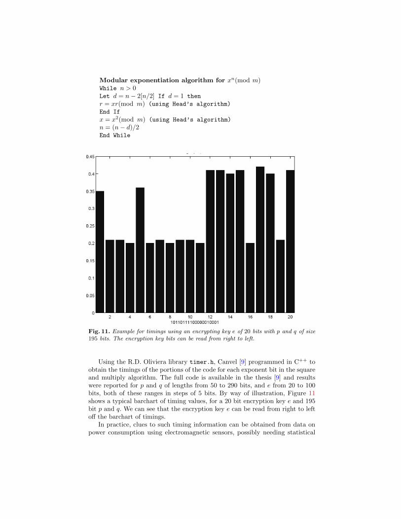
Modular exponentiation algorithm for xn(mod m)While n > 0Let d = n− 2[n/2] If d = 1 then

r = xr(mod m) (using Head’s algorithm)

End If

x = x2(mod m) (using Head’s algorithm)

n = (n− d)/2End While

Fig. 11. Example for timings using an encrypting key e of 20 bits with p and q of size195 bits. The encryption key bits can be read from right to left.

Using the R.D. Oliviera library timer.h, Canvel [9] programmed in C++ toobtain the timings of the portions of the code for each exponent bit in the squareand multiply algorithm. The full code is available in the thesis [9] and resultswere reported for p and q of lengths from 50 to 290 bits, and e from 20 to 100bits, both of these ranges in steps of 5 bits. By way of illustration, Figure 11shows a typical barchart of timing values, for a 20 bit encryption key e and 195bit p and q. We can see that the encryption key e can be read from right to leftoff the barchart of timings.

In practice, clues to such timing information can be obtained from data onpower consumption using electromagnetic sensors, possibly needing statistical

processes to clean the data of noise. A practicable defence is to obscure thepower usage data on timing information by spurious other processes. Then theeffectiveness of such obscuring techniques can be evaluated using analyses of thedistributions associated with time series from power usage. For example, a timeseries of power consumption using appropriately chosen thresholding and inter-val windows would yield a barchart and that would ideally be like that arisingfrom Poisson processes, which for a given mean are maximally disorderd [34]. In-formation geometry can be used to measure differences from the Poisson model,equivalently from its associated exponential distribution. Figure 11, shows theactual timing data of binary digits in the encryption key, illustrating preciselythe opposite of maximal disorder: a binary barchart revealing the digit sequence.

7 Dimensionality reduction methods

A general class of methods used to represent high-dimensional datasets is calledmultidimensional scaling or dimensionality reduction. In many real world prob-lems we encounter high dimensionality in large data sets and often do not knowthe optimal net probability density function family for the features representedin the data. A fundamental problem in the identification of probability densitiesfrom large multidimensional data sets, that of efficient dimensionality reduction,was addressed by Carter and his co-workers [12,11,13,14]. They used informationgeometry to obtain nearest neighbour distances by means of geodesic estimatessubordinate to a Fisher information metric.

This method takes account of the curved geometry of the data set, ratherthan displaying it as uncurved in a Euclidean geometry cf. [11], Figure 3.2. Thesignificance is that the non-obvious global topology of frequency connectivityin the data is revealed by the geodesics. An illustration using router traffic onthe Abilene network showed how anomalous behaviour unseen by local methodscould be picked up through dimensionality changes cf. [11], Figure 3.10. More-over, in document classification, the information metric approach outperformedstandard Principal Component Analysis and Euclidean embeddings [12], and itoutperformed traditional approaches to video indexing and retrieval with realworld data [16].

Such information geometric methods could extend to anomaly detection usinglarge sample size data sets derived from an underlying probability distribution inwhich the parameterization is unknown. A comparison of relevant informationtheoretic measures that are important for anomaly detection can be found inLee and Xiang [43]. Raginsky et al [48] provided a filtering and hedging jointapproach to the detection of anomalies in sequentially observed noisy data, bycomparing the current belief against a time-varying and data-adaptive threshold.The threshold is adjusted based on the available feedback from an end user.The thesis of Liu [44] addressed the problem of intrusion detection for wirelessnetworks and developed a hybrid anomaly intrusion detection approach, basedon two data mining techniques, association-rule mining and cross-feature mining.

The methods described by Carter et al [12,11] reduce the dimensionality ofdata sets and hence identify clustering of sets with similar features through 3-dimensional rendering of the resultant plots. In our case we anticipate a largedata set X1, X2, .., XN of distributions which represent to differing degrees fea-tures relating to potential cyber attacks. Such data may be collected automati-cally and routinely, with the objective of identifying anomalous behaviour asso-ciated with attempted cyber attacks. The analytic procedure consists of a seriesof computational steps:

1. Compute mutual ‘information distances’ D(i, j) among the members of thedataset of distributions X1, X2, .., XN .

2. The array of N×N differences D(i, j) is a symmetric positive definite matrixwith diagonal zero. Centralize this by subtracting row and column means andthen adding back the grand mean to give CD(i, j).

3. The centralized matrix CD(i, j) is again symmetric positive definite withdiagonal zero. Its N eigenvalues ECD(i) are necessarily real, and there areN corresponding N -dimensional eigenvectors V CD(i).

4. Let A be the 3 × 3 diagonal matrix of the first three eigenvalues of largestabsolute magnitude and let B be the 3 × N matrix of the correspondingeigenvectors. The matrix product A·B yields a 3×N matrix and its transposeis an N×3 matrix T, which gives us N coordinate values (xi, yi, zi) to embedthe N samples in R3.

In the case when no obvious model family of distributions is available, Step 1above could be effected by means of the widely used Kullback-Leibler measureof relative entropy [41,40] which in symmetrized form for two probability densityfunctions f1, f2 defined on Ω ⊆ Rn is

DKL(f1, f2) =1

2

(∫Ω

f1 log

(f1f2

)+

∫Ω

f2 log

(f2f1

))(41)

and for numerical, normalized frequency distributions F,G with bin indexing Jwe could use the discrete form

DKL(F,G) =1

2

∑j∈J

Fj log

(FjGj

)+∑j∈J

Gj log

(GjFj

) . (42)

See Johnson and Sinanovic [38] for more symmetrizing options with the Kullback-Leibler relative entropy. We note that for such an empirical frequency distribu-tion F the entropy is

S(F ) =∑j∈J

Fj . (43)

The kind of data sets collected by security monitoring software is usually cus-tomized to the context and network connectivity to be protected. Gu et al [33]used maximum entropy (43) and relative entropy (ie Kullback-Leibler (42)) tocompare a pre-trained baseline distribution for internet traffic with the current

traffic being monitored; their results indicated some success in anomaly detec-tion, including synchronizing (SYN) attacks and port scanning reconnaissanceattacks. Lee and Xiang [43] discuss intrusion detection systems, such as Sun-SHIELD [53] and tcdump [37], which collect system and network activity dataand analyse it to determine whether an attack is in progress.

Carter’s thesis [11] included an illustration using router traffic on the Abilenenetwork that showed how anomalous behaviour unseen by local methods couldbe picked up through dimensionality changes cf. [11], Figure 3.10. The data wasfrom the Abilene Network of 11 routers which comprise the core of the ‘edu’network; the number of packets on each of these routers was taken every 5minutes through 1-2 January 2005, which yielded an 11-dimensional dataset of576 samples.

Some illustrations of applications of dimensionality reduction to stochastictextures in one and two dimensional processes can be found in [26]. An exam-ple of a 1-dimensional stochastic texture is a grey-level barcode for a genome,obtained by mapping the 20 amino acids onto grey levels. The neighbourhoodstructure of grey-level values yielded autocovariances and hence multivariateGaussian distributions; then the dimensionality reduction of a large dataset ofthese could be represented on a plot in R3 which illustrated the main featuresdiscriminating among yeast, human, and randomly-generated genomes, cf. [26]Figures 16 and 17. Two-dimensional stochastic textures can be represented assurface topographies and these were studied in [24].

Autocovariance extractions can be made from administratively monitoredtime series for a local network of nominally secure access points to a serverproviding sensitive data. Then for the case of k variables arising from valuex1 at a point t1 and the value of the succession of averages of its successiveneighbours at distances giving x2 at t±2 and so on to xk at t±k in the series, wecan compute analytically the information distance D(ΣA, ΣB) between pairs ofk × k covariance matrices ΣA, ΣB from §2.2

D(ΣA, ΣB) =

√√√√1

2

k∑j=1

log2(λABj ) (44)

where λABj = Eig(SAB) and SAB = ΣA−1/2 ·ΣB ·ΣA−1/2. (45)

Multivariate monitoring data in n-dimensional pixel form can be similarly treatedthrough its autocovariance matrices, the only difference being that the neigh-bours for a given pixel (xi) ∈ Rn form annular regions of radius 1, 2, . . . , k aroundthe pixel [24].

In the case that the data is more complex, for example mixtures of multivari-ate Gaussians, analytic information distances are not available but approxima-tions have been obtained, for example in [22] where also the effects of differentweighting sequences were investigated. In many applications, a true informa-tion metric is not essential since relative discriminations that are monotonicallyrelated to it may be adequate for purposes of comparison between datasets.

8 Discussion

The framework of Riemannian geometry has been enormously valuable in thedevelopment over the past century and a half of physical models for real pro-cesses in time and space, as well as in the abstract high-dimensional and infinite-dimensional spaces that are important for physical field theories. Conversely,these developments in physical models have stimulated developments in geom-etry, global analysis and functional analysis, to extend mathematical structuresto contexts that were not previously envisaged. The more recent developmentof cheap computer power and rapid processing has made possible very effec-tive developments in computational geometry for numerical solution of complexproblems.

Analytic computing packages like Mathematica [54] enable rapid handling ofcomplex operations in large numbers of variables to obtain analytic solutionsto mathematical problems that were previously inaccessible. Moreover, this ana-lytic work is easily performed by anyone with experience in writing mathematicalexpressions and it is easy to display results and effects of variables graphically,including with animation. The development during the last seventy years of in-formation geometry has provided all the tools of Riemannian geometry, for useon smoothly parametrized families of probability density functions, and mod-ern computational information geometry makes possible the analysis of complexstatistical models. Moreover, it provides their representation through naturalembeddings such as Figures 2, 4, 6, which are more easily interpreted than ta-bles of data.

Encoding and decoding algorithms for public key encryption typically involverepeated numerical exponentiation procedures. Correlations, between power con-sumption and data bit values, during processing by a device when supplied withchosen inputs can reveal clues to the encryption key, if a sensor can be placedto pick up the power consumption traces, §6. This stems from the fact that theprocessing algorithms use different times to run for steps involving a ‘1’ bit froma ‘0’ bit in the key, as we illustrated using modular exponentiation with Head’salgorithm in Figure 11 above, from our report of timing studies in [10]. Onepracticable defence is to obscure the power usage data on timing informationby spurious other processes. Then the effectiveness of such obscuring techniquescan be evaluated using analyses of the distributions associated with time seriesfrom power usage. For example, a time series of power consumption using ap-propriately chosen thresholds and interval windows would yield a barchart thatwould ideally be like that arising from Poisson random processes, hiding anyinfluence from internal process timings. In evaluating such obscuring techniques,information geometry can measure differences from the Poisson ideal.

The monitoring of networks to identify breaches of cyber security may ofteninvolve the automated collection of very large volumes of possibly high dimen-sional time series data, which may be representable through empirical frequencydistributions tailored to the process to be protected. In some cases these dis-tributions may be interpreted as perturbations of, for example, Poisson randomprocesses or uniform processes, which could be an ideal target for the data in

the absence of attacks or anomalous events. We have seen in §3 that the familyof gamma distributions and its logarithmic version have relevance to this con-text. These have simple information geometry, which we have illustrated in someexample calculations, §5, concerning the measurement of departures from unifor-mity and from a Poisson random process. There also we showed how to providea distance between two nearby truncated Gaussian-like distributions, Figure 10.For automated security monitoring of sample distributions, these distance valuescan be used for creating alerts or initiating action when certain chosen thresholddeviations arise from target uniform or chosen truncated Gaussian distributions.In the absence of a model family of distributions we can use the symmetrizedKullback-Leibler relative entropy expression, equation (42), to measure distancebetween empirical frequency distributions.

In other cases, for n-dimensional data values (xi) ∈ Rn for any n = 1, 2, . . . ,we can compute (k × k) autocovariance matrices from values at a point in Rnand the averages of its jth-neighbours for a set of j = 1, 2, . . . , k. These areamenable to an interpretation through the information geometry of k-variateGaussian covariances, which also have relatively simple information geometry aswe showed in §2.2 where we have provided explicit analytic expressions, equation(44) for distances between two (k × k) covariance matrices.

For the situations when large numbers of empirical or fitted distributions haveto be handled, we have described explicitly in §7 the steps to follow in the methodof dimensionality reduction. The methodology represents all of the datasets onone plot in R3, which reveals the topology of the dataset and any prominentfeatures, such as clusters and natural subgroups within the data, regardless ofthe number of datasets. This procedure has been shown to outperform the morecommon Principal Component Analysis [12] in feature identification.

References

1. S-I. Amari. Theory of Information Spaces—A Geometrical Foundation of the Analy-sis of Communication Systems. Research Association of Applied Geometry Memoirs4 (1968) 171-216.

2. S-I. Amari. Differential Geometrical Methods in Statistics Springer LectureNotes in Statistics 28, Springer-Verlag, Berlin 1985.

3. S-I. Amari, O.E. Barndorff-Nielsen, R.E. Kass, S.L. Lauritzen and C.R. Rao. Dif-ferential Geometry in Statistical Inference. Lecture Notes Monograph Series,Institute of Mathematical Statistics, Volume 10, Hayward California, 1987.

4. S-I. Amari and H. Nagaoka: Methods of Information Geometry. Oxford, AmericanMathematical Society, Oxford University Press (2000).

5. K. Arwini and C.T.J. Dodson: Information Geometry Near Randomness and NearIndependence. Lecture Notes in Mathematics. New York, Berlin, Springer-Verlag(2008).

6. C. Atkinson and A.F.S. Mitchell. Rao’s distance measure. Sankhya: Indian Journalof Statistics 48, A, 3 (1981) 345-365.

7. E. Byrse and D. Leversage: The Industrial Security Incident Database. (2006)http://www.securitymetrics.org/attachments/Metricon-1-Leversage-Rump.pdf

8. E. Byrse and J. Lowe: The Myths and Facts behind Cyber Security Risks for In-dustrial Control Systems. VDE 2004 Congress, VDE, Berlin, October 2004

9. B. Canvel. Timing Tags for Exponentiations for RSA. MSc Thesis, Depart-ment of Mathematics, University of Manchester Institute of Science and Technology,Manchester (1999).

10. B. Canvel and C.T.J. Dodson. Public Key Cryptosystem Timing Analysis.CRYPTO 2000, Rump Session Santa Barbara, 20-24 August 2000.http://www.maths.manchester.ac.uk/~kd/PREPRINTS/rsatim.pdf 27 August 2000

11. K.M. Carter. Dimensionality reduction on statistical manifolds. PhD thesis, Uni-versity of Michigan, 2009. http://tbayes.eecs.umich.edu/kmcarter/thesis

12. K.M. Carter, R. Raich and A.O. Hero III. FINE: Information embed-ding for document classification. In Proc. 2008 IEEE International Confer-ence on Acoustics, Speech, and Signal Processing, Las Vegas, March 2008.http://tbayes.eecs.umich.edu/kmcarter/fine_doc

13. K.M. Carter, R. Raich,W.G. Finn and A.O. Hero III. Fisher information nonpara-metric embedding. IEEE Trans. Pattern. Anal. Mach. Intell. 31 (2009) 20932098.http://arxiv.org/abs/0802.2050v1

14. K.M. Carter, R. Raich,W.G. Finn and A.O. Hero III. Information-geometric di-mensionality reduction. IEEE Signal Processing Mag. 99 (2011) 89-99.http://web.eecs.umich.edu/~hero/Preprints/carter_spsmag_igdr_rev3.pdf

15. S. Chari, C.S. Jutla, J.R. Rao and P. Rohatgi. Towards sound approaches to coun-teract power-analysis attacks. In Advances in Cryptology-CRYPTO ’99, Ed.M. Wiener, Lecture Notes in Computer Science 1666, Springer, Berlin 1999 pp 398-412.

16. X. Chen and A. Hero. Fisher Information Embedding for Video Indexing andRetrieval. SPIE Electronic Imaging Conference, San Jose, 2011.nts/ChenEI11.web.eecs.umich.edu/~hero/Prepripdf

17. J. Chen and G. Venkataramani: An algorithm for detecting contention-based coverttiming channels on shared hardware. In Proc. HASP ’14 Third Workshop onHardware and Architectural Support for Security and Privacy ACM Dig-ital Library dl.acm.org http://www.seas.gwu.edu/~guruv/hasp14.pdf

18. CPNI: UK Centre for the Protection of National Infrastructurehttp://www.cpni.gov.uk/advice/cyber/

19. P. Crzegorzewski and R. Wieczorkowski. Entropy-based goodness-of-fit test forexponentiality. Commun. Statist. Theory Meth. 28, 5 (1999) 1183-1202.

20. N.J. Daras: Stochastic analysis of cyber attacks. In Applications of Mathematicsand Informatics in Science and Engineering, Springer Optimization and its Appli-cations 91, Ed. N.J. Daras, 105–129 (2014)

21. C.T.J. Dodson Editor. Proceedings of Workshop on Geometrization of Sta-tistical Theory Lancaster 28-31 October 1987, ULDM Publications, University ofLancaster, 1987.

22. C.T.J. Dodson. Information distance estimation between mixtures of multivariateGaussians. Presentation at Workshop on Computational information geometryfor image and signal processing ICMS Edinburgh, 21-25 September 2015.

23. C.T.J. Dodson. Some illustrations of information geometry in biology and physics.In Handbook of Research on Computational Science and Engineering: Theory andPractice Eds. J. Leng, W. Sharrock, IGI-Global, Hershey, PA, 2012, pp 287-315.http://www.igi-global.com/book/handbook-research-computational-science-engineering/51940

24. C.T.J. Dodson, M. Mettanen and W.W. Sampson: Dimensionality reduction forcharacterization of surface topographies. Presentation at Workshop on Computa-tional information geometry for image and signal processing ICMS Edin-burgh, 21-25 September 2015.

25. C.T.J. Dodson and T. Poston. Tensor Geometry Graduate Texts in Mathematics130, Second edition, Springer-Verlag, New York, 1991.

26. C.T.J. Dodson and W.W. Sampson: Dimensionality reduction for classification ofstochastic texture images In F. Nielsen(Ed.): Geometric Theory of Information.Springer, Heidelberg, 1013–1015 (2014)

27. C.T.J. Dodson and S.M. Thompson. A metric space of test distributions for DPAand SZK proofs. Poster Session, Eurocrypt 2000, Bruges, 14-19 May 2000.http://www.maths.manchester.ac.uk/~kd/PREPRINTS/mstd.pdf

28. P.S. Eriksen. Geodesics connected with the Fisher metric on the multivariate nor-mal manifold. In C.T.J. Dodson, Editor, Proceedings of the GST Workshop,Lancaster (1987), 225-229. http://trove.nla.gov.au/version/21925860

29. W. Feller: An Introduction to Probability Theory and its Applications. Volume II2nd Edition, Wiley, New York (1971).

30. R.A. Fisher. Theory of statistical estimation. Proc. Camb. Phil. Soc. 122 (1925)700-725.

31. P. Ginlin. Primes and Programming: An Introduction to Number Theorywith Computing. Cambridge University Press, 1993.

32. O. Goldreich, A. Sahai and S. Vadham. Can Statistical Zero-Knowledge be madenon-interactive? Or, on the relationship of SZK and NISZK. In Advances inCryptology-CRYPTO ’99, Ed. M. Wiener, Lecture Notes in Computer Science1666, Springer, Berlin 1999 pp 467-484.

33. Y. Gu, A. McCallum and D. Towsley: Detecting anomalies in network traffic us-ing maximum entropy estimation. In Proc. Internet Measurement Conference2005 pp 345-350. More details are in the Technical Report from the Department ofComputer Science, UMASS, Amherst 2005.

34. F.A. Haight. Handbook of the Poisson Distribution J. Wiley, New York,1967.

35. USA Homeland Security: Cybersecurity, http://www.dhs.gov/topic/cybersecurity2015.

36. T-Y. Hwang and C-Y. Hu: On a characterization of the gamma distribution: Theindependence of the sample mean and the sample coefficient of variation. AnnalsInstitute Statistical Mathematics 51(4) 749-753 (1999).

37. V. Jacobson, C. Leres and S. McCanne: tcdump via anonymous ftp.ee.lbl.gov, June1989.

38. D.H. Johnson and S. Sinanovic: Symmetrizing the Kullback-Leibler Distance. RiceUniversity doc https://scholarship.rice.edu/handle/1911/19969

39. P. Kocher, J. Jaffe and B.Jun. Differential Power Analysis. In Advances inCryptology-CRYPTO ’99, Ed. M. Wiener, Lecture Notes in Computer Science1666, Springer, Berlin 1999 pp 388-397.

40. S. Kullback. Information Theory and Statistics. Wiley, New York, 1959.41. S. Kullback and R. A. Leibler. On information and sufficiency. Ann. Math. Stat.,

22 (1951) 79-86.42. R.G. Laha: On a characterization of the gamma distribution. Ann. Math. Stat. 25

(1954) 784-787.43. W. Lee and D. Xiang. Information-theoretic measures for anomaly detec-

tion. In Proc. IEEE Symposium Security and Privacy (2001) pp 130-143.10.1109/SECPRI.2001.924294

44. Y. Liu: Intrusion detection for wireless networks. PhD thesis, Stevens Institute ofTechnology, ACM Digital Library dl.acm.org .

45. E. Nash: Hackers bigger threat than rogue staff. VNU Publications, May 15, 2003.46. F. Nielsen and F. Barbaresco (Eds.): Geometric Science of Information

GSI2013, LNCS 8085, Springer, Heidelberg (2013).47. F. Nielsen(Ed.): Geometric Theory of Information. Springer, Heidelberg

(2014).48. Maxim Raginsky, Rebecca Willett, Corinne Horn, Jorge Silva and Roummel Mar-

cia: Sequential anomaly detection in the presence of noise and limited feedback.ArXiv arXiv:0911.2904v4 (2012) 1-19.

49. C.R. Rao. Information and accuracy attainable in the estimation of statisticalparameters. Bull. Calcutta Math. Soc. 37, (1945) 81-91.

50. A. Rushkin, J. Soto et al. A Statistical Test Suite for Random and Pseu-dorandom Number Generators for Cryptographic Applications. NationalInstitute of Standards & Technology, Gaithersburg, MD USA, 2001.

51. B.Ya. Ryabko and V.A. Monarev. Using information theory approach to random-ness testing. J. Stat. Plan. Inf. 133, 1 (2005) 95-110.

52. S.D. Silvey. Statistical Inference Chapman and Hall, Cambridge 1975.53. SunSoft SunSHIELD Basic Security Module Guide. Soft, Mountain View,

CA, 1995. https://docs.oracle.com/cd/E19457-01/801-6636/801-6636.pdf54. S. Wolfram. The Mathematica Book 3rd edition, Cambridge University Press,

Cambridge, 1996.