On Selmer Groups of Geometric Galois …people.math.umass.edu/~weston/papers/sgggr.pdfOn Selmer...
170
On Selmer Groups of Geometric Galois Representations Tom Weston Department of Mathematics, Harvard University, Cambridge, Mass- chusetts 02140 E-mail address : [email protected]
Transcript of On Selmer Groups of Geometric Galois …people.math.umass.edu/~weston/papers/sgggr.pdfOn Selmer...

On Selmer Groups of Geometric
Galois Representations
Tom Weston
Department of Mathematics, Harvard University, Cambridge, Mass-
chusetts 02140
E-mail address: [email protected]


iii
Dedicated
to the memory of Annalee Henderson
and to Arnold Ross


Contents
Introduction ixAcknowledgements xii
Notation and terminology xvFields xvCharacters xvGalois modules xvSchemes xvSheaves xviCohomology xviK-theory xvi
Part 1. Selmer groups and deformation theory 1
Chapter 1. Local cohomology groups 31. Local finite/singular structures 32. Functorialities 43. Local exact sequences 54. Examples of local structures 65. Ordinary representations 76. Cartier dual structures 87. Local structures for archimedean fields 9
Chapter 2. Global cohomology groups 111. Selmer groups 112. Functorialities 133. The global exact sequence 134. A finiteness theorem for Selmer groups 145. The Kolyvagin pairing 166. Shafarevich-Tate groups 187. The Bockstein pairing 20
Chapter 3. Annihilation theorems for Selmer groups 211. Partial geometric Euler systems 212. The key lemmas 223. The annihilation theorem 254. Right non-degeneracy of the Bockstein pairing 275. A δ-vanishing result 28
Chapter 4. Flach systems 311. Minimally ramified deformations 31
v

vi CONTENTS
2. Tangent spaces and Selmer groups 343. Good primes 364. Flach systems 385. Cohesive Flach systems 396. Cohesive Flach systems of Eichler-Shimura type 40
Chapter 5. Flach systems of Eichler-Shimura type 431. The map on differentials 432. The Tate pairing 453. A special case 474. A matrix computation 525. Computation of Ξ in the non-diagonal case 536. Computation of Ξ in the general case 54
Part 2. Construction of cohesive Flach systems 55
Chapter 6. The Flach map 571. The coniveau spectral sequence in etale cohomology 572. The localization sequence 593. Grothendieck’s purity conjecture 614. The coniveau spectral sequence in K-theory 625. Definition of the Flach map 646. Functoriality and passage to the limit 667. Functoriality II 67
Chapter 7. Local analysis of the Flach map 711. Overview 712. Local behavior I 723. Local behavior II 724. Local behavior III 745. The divisor map 756. The cycle map 777. Relations with Galois cohomology 788. Functoriality and passage to the limit 789. Example : Schemes over global fields 7910. Local behavior at places over l 80
Chapter 8. Flach classes for correspondences 831. Algebraic correspondences 832. Correspondences and operations on etale cohomology 843. Composition of correspondences 864. Marked varieties 885. Divisors and compositions 896. The Leibniz relation 907. Algebras of correspondences 928. Derivations in the self-adjoint case 939. Local diagrams in the self-adjoint case 9410. Derivations in the general case 9511. Untwistings and cycle classes 9712. Derivations modulo η 97

CONTENTS vii
Chapter 9. Construction of geometric Euler systems 991. Divisorial liftings of cycles 992. Construction of partial Euler systems 1003. Partial Euler systems on products 1014. Construction of Flach systems in the self-adjoint case 1025. Construction of Flach systems in the general case 1056. Construction of cohesive Flach systems 106
Part 3. Examples 107
Chapter 10. The modular curve X0(N) 1091. The geometry of X0(N) 1092. The modular unit ∆ 1133. The divisor of fp in positive characteristic 1154. The cohesive Flach system 116
Chapter 11. The modular curve X1(N) 1171. The geometry of X1(N) 1172. Admissible markings 1203. The cohesive Flach system 121
Chapter 12. Kuga-Sato varieties 1231. The geometry of Kuga-Sato varieties 1232. Admissible markings 1253. The cohesive Flach system 1264. Applications 126
Appendix 129
Appendix A. Edge maps of spectral sequences 1311. Notation for filtered complexes 1312. Edge maps 1323. Edge maps in spectral sequences of filtered complexes 1334. Edge maps in Grothendieck spectral sequences I 1345. Edge maps in Grothendieck spectral sequences II 1356. Boundary maps of exact sequences of filtered complexes 1367. Boundary maps of Grothendieck spectral sequences 1378. Edge maps of exact couples 138
Appendix B. Gorenstein linear algebra 1411. Definitions 1412. Gorenstein traces and congruence elements 1423. Gorenstein duality 1434. Gorenstein pairings 1445. Skew-symmetric Gorenstein pairings 1456. Bilateral derivations 1467. Torsion modules 148
Bibliography 151


Introduction
Fix a squarefree integer N and let f be a rational weight 2 newform for Γ0(N).Let H be the l-adic representation associated to f for some l ≥ 7; H is a freeZl-module of rank 2. Let QS denote the maximal extension of Q unramified awayfrom Nl and set GQS
= Gal(QS/Q). Flach proved the following theorem regardingthe deformation theory of H. (See [Wes00, Appendix A] for the proof that theset of primes satisfying Flach’s conditions has density 1; this set can be given quiteexplicitly.)
Theorem 0.1 ([Fla92]). Fix f as above and assume that f does not havecomplex multiplication. Then the set of primes l such that the universal deforma-tion ring of the residual representation ρ : GQS
→ AutFl(H/lH) is isomorphic toZl[[T1, T2, T3]] has density 1.
This result was extended to the case of newforms defined over arbitrary numberfields in [Fla95] and [Maz]. In this case the l-adic representation H is free of rank2 over a certain completion A of a Hecke algebra; this ring A is a reduced, finite,flat, local, Gorenstein Zl-algebra and contains a Hecke operator Tp for every primep. Let k denote the residue field of A. Mazur observed that Flach’s constructioncan be used to obtain results on the Taylor-Wiles deformation problem for almostall l ≥ 7 not dividing N .
Theorem 0.2 ([Maz]). Let f be a newform of weight 2 for Γ0(N). Let l ≥ 7be a prime not dividing N and let H be the l-adic representation associated to f .Assume that the natural map GQ → Autk(H ⊗A k) is surjective. Let R be theminimally ramified universal deformation ring for H ⊗A k. Then R is a finiteA-algebra and the natural map R → A induces an isomorphism of differentialsΩR ⊗R A→ ΩA.
In this thesis I extend the results of Flach and Mazur to the case of (most)newforms of weight at least 2 for Γ1(N). I also show that the “geometric Eulersystem” used to prove these results has a very rich algebraic structure and thatthe isomorphism it yields in deformation theory is essentially canonical. The mainresult in this context can be phrased as follows.
Theorem 0.3 (Theorem XII.3.1 and Theorem IV.6.2). Let f be a newform ofweight k ≥ 2 for Γ1(N). Let l ≥ max7, k be a prime not dividing N and let Hbe the l-adic representation (over an appropriate completion A of a Hecke algebra)associated to f . Assume that f can be “cleanly realized” in the cohomology of theuniversal elliptic curve with level N -structure (see Chapter XII for precise condi-tions). Set T = End0
AH(1) and assume that the natural map GQ → Autk(H ⊗A k)is surjective. Let R be the minimally ramified universal deformation ring for H⊗Ak(see Section IV.1). Then R is a finite A-algebra and the natural map R → A in-duces an isomorphism of differentials ΩR⊗RA→ ΩA. Furthermore, the inverse of
ix

x INTRODUCTION
this isomorphism is characterized by the fact that the identification
ΩA → ΩR ⊗R A ∼= HomZl
(H1f (Q, T ∗[η]),Ql/Zl
)(see Section IV.2) identifies the differential of Tp ∈ A with −12 times the imageunder the Bockstein pairing
H1f (Q, T/ηT )→ HomZl
(H1f (Q, T ∗[η]),Ql/Zl
)of the cohomology class cp ∈ H1
f (Q, T/ηT ) obtained via the Flach construction.Here H1
f (Q, ·) is a Selmer group (see Section II.1), T ∗ is the Cartier dual of T ,and η is the congruence element (see Appendix B.2) for the Gorenstein Zl-algebraA.
However, it is natural to hope that the method of proof of these results isas interesting as the results themselves. For this reason we proceed in as muchgenerality as we can. Let X be a nonsingular algebraic variety over a global fieldF and let H be a quotient of the etale cohomology group H2m(XFs ,Zl(m + 1))for some m. I give a “general” method (contingent on the existence of appropriategeometric data onX×X) for the production of geometric Euler systems for End0
AH;these in turn yield corresponding annihilators of certain Selmer groups. Theseannihilators yield results on the deformation theory of the Galois representationH/lH. Somewhat more generally one can hope to use appropriate geometric dataon X itself to control the Selmer group of H; this could then possibly be related tothe Bloch-Kato conjectures.
The required geometric data (in the deformation theory case) does exist formodular curves and Kuga-Sato varieties. It seems likely that it exists in the caseof Hilbert modular surfaces as well. One can give “explicit” conditions for theexistence of this data in general, although at this point these are not particularlyuseful.
We now discuss the contents of this thesis in more detail. The first five chap-ters concern Selmer groups and geometric Euler systems in Galois cohomology. Thematerial of the first three chapters is presented in a fair amount of generality; Chap-ters IV and V are focused on the specific Taylor-Wiles deformation problem. Thematerial of the first two chapters is essentially standard, although our presentationis a synthesis of several others.
Chapter I concerns local conditions on Galois cohomology. We define suchconditions in full generality in preparation for later results. We especially focus onthe functorial aspects of these conditions. We also include the explicit computationof the “natural” local condition in the case of ordinary representations.
Chapter II is the globalization of Chapter I: we use local conditions at everyplace to define Selmer groups of Galois modules. After establishing appropriatefunctorialities we turn to the definition of two pairings which play a crucial role inour work. The first, the Kolyvagin pairing, combines local and global information.We prove that in a certain sense this pairing evaluates how far a collection oflocal cohomology classes are from arising from a global cohomology class. Thesecond pairing, the Bockstein pairing, is a pairing between Selmer groups which isof independent interest in many circumstances.
In Chapter III we define the notion of a partial geometric Euler system andprove the corresponding annihilation theorems for Selmer groups via the Kolyvaginpairing and the Tchebatorev density theorem. We also give an application of these

INTRODUCTION xi
methods to prove the non-degeneracy of the Bockstein pairing in the presence of anEuler system. These results are all based on the ideas of Thaine and Kolyvagin, asrefined by Flach, Mazur and Rubin. Our presentation is marginally more generalthan others, but otherwise is well-known.
Chapter IV concerns Mazur’s notions of full geometric Euler systems. We beginby considering the deformation theory of certain rank 2 Galois representations overZl-algebras A and explain the connection with Selmer groups. We then define thenotion of a Flach system, which is a slightly strengthened partial geometric Eulersystem. The real refinement comes with Mazur’s cohesive Flach systems, whichcombine Flach systems with some additional global algebraic structure. This addi-tional structure results in much more precise deformation theoretic consequences.We then refine this further with our new notion of a cohesive Flach system ofEichler-Shimura type; these are cohesive Flach systems with sharply specified localbehavior.
One can pass via the Bockstein pairing and a cohesive Flach system to a certaincomplicated pairing between the differentials ΩA and their dual. In Chapter V wegive a computational proof that in the case of a cohesive Flach system of Eichler-Shimura type this pairing is nothing more than a scalar multiple of the canonicalduality pairing. This is mostly straightforward except for the computation of thelocal invariant map and a certain matrix lemma.
The second part of this thesis concerns the production of geometric Euler sys-tems for the etale cohomology of varieties over number fields. The central tool,which we call the Flach map, originated in the work of Flach. Our description isa generalization of that of [Fla95] to higher dimensional varieties. [Maz] providedan alternate description in the low-dimensional case; this description does not makedirect use of algebraic K-theory. We have not adopted this approach as it does notseem to easily generalize to higher dimensions.
The Flach map is defined in Chapter VI, after some preliminaries on theconiveau spectral sequence in etale cohomology and algebraic K-theory. We de-fine the Flach map for smooth separated schemes X over any perfect field and oversome non-perfect fields as well; it is a map from certain pairs of cycles and functionson X to the Galois cohomology of the etale cohomology of X. The description ofthese cycles and functions is most straightforward over local and global fields.
In Chapter VII we give the fundamental local description of the Flach mapfor a variety X over a global field. Specifically, we prove that at places of goodreduction one can test a Galois cohomology class against an appropriate unramifiedlocal condition via a certain divisor map to the Chow groups of X. (Flach proveda similar result for products of elliptic curves in [Fla92]; he offered a result forproducts of modular curves in [Fla95], although the proof there is incomplete.)The proof of this theorem makes use of certain results from higher algebraic K-theory; the statement, however, does not involve any explicit K-theory. Assuminga detailed knowledge of the geometry of X, this makes it possible to use the Flachmap to generate partial geometric Euler systems; this is the subject of Chapter IX.We also give a result of Flach concerning the local behavior of the Flach map tol-adic cohomology at places above l.
Chapter VIII concerns certain algebraic structures on the Flach map for prod-ucts X × X. After some preliminary discussion of algebraic correspondences, weprove the fundamental Leibniz relation of Mazur and Beilinson. Their argument

xii INTRODUCTION
for this relation for curves used a clever reduction to a trivial case. We insteadpresent a more direct proof which is valid in arbitrary dimension. We then explainhow to use the Leibniz relation to generate a system of Galois cohomology classeswhich have the algebraic structure of a cohesive Flach system. This involves thetheory of Gorenstein rings and bilateral derivations as developed in Appendix B.
Chapter IX combines the results of Chapter VII and Chapter VIII to give somesample theorems for the production of geometric Euler systems. In all cases wemust assume the existence of appropriate geometric data. The ideas of SectionIX.3 were inspired by [?] and [?], although these papers do not explicitly appearanywhere in the discussion.
The last three chapters are the applications of the methods we have developed tomodular forms. Chapter X concerns the case of the modular curveX0(N). We makesome auxiliary hypotheses on the Hecke algebra to simplify the exposition; withthese in place the construction is straightforward. (The existence of the cohesiveFlach system in this case is due to Mazur.) These restrictions are removed viathe more general results on X1(N) in Chapter XI. In Chapter XII we use therealization of Galois representations for modular forms of higher weight in thecohomology of open Kuga-Sato varieties to construct the cohesive Flach system.This requires some slight extensions of the results of Chapters VII and VIII to thissetting. Otherwise the construction is completely analogous to the previous cases.The constructions of Chapters XI and XII are new, although in some cases thedeformation theoretic conclusions are weaker than those of [?] (for the weight 2case) and upcoming work of Diamond (for the higher weight case).
We include two appendices. The first concerns compatibilities of edge mapsof spectral sequences; this is mostly well-known but is included here for lack of anadequate reference. Appendix B is a discussion of the linear algebra of modules overGorenstein rings. We also give an introduction to the theory of bilateral derivations.
Acknowledgements
This thesis could not have been written without a tremendous amount of helpfrom my advisor, Barry Mazur. He has always been extremely willing to share hisideas and insights with me; I can only hope that his point-of-view is visible in thiswork.
There are many people who (for no obvious reason) invested a lot of time inhelping me through this thesis. I must especially thank Brian Conrad, Mark Dickin-son, Matthew Emerton and Robert Pollack for their constant help, both answeringmy questions and working through confusing points with me. I would also like tothank Fred Diamond, Benedict Gross, Joe Harris, Karl Rubin and Richard Tay-lor for numerous helpful conversations, both mathematical and otherwise. I havebeen very fortunate to have had the opportunity to learn mathematics from manydifferent people; in particular, I would like to thank Matt Baker, Keith Conrad,Jordan Ellenberg, Wee-Teck Gan, Tom Graber, Tomas Klenke, Adam Logan, ElenaMantovan, Adi Ofer, David Pollack, David Savitt, Jason Starr and Sam Williamsfor their help.
I, like all Harvard mathematics graduate students, have been extremely fortu-nate to have the support of a very helpful and dedicated administrative staff. Iwould especially like to thank Donna D’Fini and Irene Minder for all of their helpover the last four years.

ACKNOWLEDGEMENTS xiii
My parents have always been extremely supportive (in every way) throughoutmy education; I hope that they know how much I have appreciated it even if Ididn’t always make it clear. My brothers Michael and Matthew have been my bestfriends for my entire life, and talking to them has often been the best way to getaway from this thesis for a while. I also want to thank Jessica Sidman; she hasput up with an inordinate amount of whining over the last year and a half. Shesomehow has still managed to answer my algebraic geometry questions and makethis entire process much more enjoyable than it had any right to be. Finally, I mustthank P.J.; his remarkable aid at a pivotal moment will always be appreciated.


Notation and terminology
Fields
Any time a field F appears in the text we assume that it is accompanied bya fixed choice of separable algebraic closure Fs. We further assume that for anyinclusion of fields F → F ′ these choices are made in such a way that Fs is a subfieldof F ′s . We write GF for the absolute Galois group Gal(Fs/F ) of F and cdF forthe Galois cohomological dimension of F . By a global field we will mean a finiteextension of Q or Fp(t) (for some prime p) and by a local field we will mean a finiteextension of Qp or Fp((t)) (for some prime p).
If k is a finite field, by a Frobenius element Fr for k we will always mean ageometric Frobenius element, normalized by Fr(x)#k = x for all x ∈ k. If X is ascheme over k, we let Fr denote the k-linear Frobenius morphism of X. If F is aglobal field and v is a place of F , we write Fr(v) for a geometric Frobenius elementof GF .
Characters
For any field F of characteristic different from l, we let Zl(1) denote the Tatemodule of the l-power roots of unity. The natural map GF → AutZl Zl(1) willbe called the cyclotomic character and denoted ε. We write Zl(−1) for the dualHomZl(Zl(1),Zl) of Zl(1).
Let F be a global field and χ : GF → A× a character. If v is a place of F atwhich χ is unramified, we write χ(v) for χ(Fr(v)). Note that ε(Fr(v)) = (#kv)−1.
Galois modules
If F is a field and T is a topological abelian group with an action of GF , wewill always assume that the GF -action is continuous for the profinite topology onGF and the given topology on T . If T is such a GF -module, we write F (T ) for thefixed field of the kernel of the map GF → AutT ; we call F (T ) the splitting field ofT over F . If T is a Zl-module with a Zl-linear action of GF and n > 0, then wewrite T (n) for the n-fold tensor product of T with Zl(1); if n < 0, we write T (n)for the |n|-fold tensor product of T with Zl(−1).
Schemes
If x is a point of a scheme X, we write k(x) for its residue field and define itscodimension, denoted codimX x, to be the dimension of the local ring OX,x. If Z isan arbitrary closed subset ofX, we define k(Z) to be the product of the residue fieldsof the minimal points of Z, and we define codimX Z to be the least codimension ofany point of Z. We write Xp for the set of points of X of codimension exactly p.If x is a point of X, we will write x for the reduced closed subscheme of X defined
xv

xvi NOTATION AND TERMINOLOGY
on the closure of x. If X is a scheme over a base S and S′ → S is any morphism,we will write XS′ for the fibre product X ×S S′. If Y and Z are two subschemes ofa third scheme X, then by the scheme-theoretic intersection of Y and Z (in X) wemean the fibre product Y ×X Z.
By a variety over a field F we will mean a reduced irreducible separated schemeof finite type over SpecF . If X and Y are varieties over a field F , then we writeX × Y for the fiber product X ×SpecF Y .
Sheaves
All sheaves other than structure sheaves are assumed to be sheaves for theetale topology unless otherwise specified; locally constant sheaves are assumed tobe locally constant for the etale topology. If i : U → X is an open immersion andF is a sheaf on X, we will usually just write F for the pullback sheaf i∗F on U . IfF is any torsion sheaf, we write F(m) for its mth Tate twist:
F(m) = F ⊗ µ⊗m∞ .
If i : X ′ → X is a morphism and F is a Tate twist of a constant sheaf on X we willusually still write F for the pullback sheaf i∗F on X ′.
Cohomology
All spectral sequences are assumed to be cohomological. All cohomology iseither etale or Galois; we will attempt to be careful as to which is which, even whenthey coincide. If L/K is an extension of fields and T is a topological Gal(L/K)-module, we write Hi(L/K, T ) for the cohomology group Hi(Gal(L/K), T ), com-puted with continuous cochains. If L is a separable algebraic closure of K, then wejust write Hi(K,T ) for these cohomology groups.
If F is an l-adic etale sheaf on a scheme X, then we write Hi(X,F) for theinverse limit of the etale cohomology groups Hi(X,F/lnF). If F is an etale sheafof Ql-vector spaces, then we write Hi(X,F) for the tensor product of Ql withHi(X,F0/l
nF0) where F0 is any l-adic subsheaf of F with F0 ⊗ Ql = F ; thisdefinition is independent of the choice of F0.
K-theory
We write Ki and K ′i for Quillen’s K-groups for the category of locally freesheaves and the category of all coherent sheaves respectively; these functors agreeon regular schemes. We will write Ki(X) for the Zariski sheaf of K-groups on X.We take all K-groups to vanish for negative indices.

Part 1
Selmer groups and deformationtheory


CHAPTER 1
Local cohomology groups
In this chapter we give the basic theory of finite/singular structures over localfields in preparation for the definition of Selmer groups in Chapter II.
1. Local finite/singular structures
Fix a prime l and let A be a finite, flat, local Zl-algebra. Let K be a localfield with residue field k of characteristic p; we allow p = l. We write Kur forthe maximal unramified extension of K, and we let IK = Gal(Ks/Kur) denote theinertia group of K.
Let T be an A-module with an A-linear action of GK . We further assume thatone of the following holds:
• T is a finitely generated Zl-module and the GK-action on T is continuousfor the l-adic topology on T ; or
• T is a torsion Zl-module of finite corank (that is, T is isomorphic as a Zl-module to (Ql/Zl)r ⊕ T ′ for some r ≥ 0 and some Zl-module T ′ of finiteorder) and the GK-action on T is continuous for the discrete topology onT .
We will be working with cohomology with continuous cochains (see [Rub00, Ap-pendix B]) and these assumptions are necessary in order to insure that it is wellbehaved. In the second case, continuous cohomology agrees with the usual profi-nite/discrete cohomology. We will refer to T as above as l-adic GK-modules overA; if T satisfies the first condition we will say that it is finitely generated, and if itsatisfies the second condition we will say that it is discrete. Note that T is bothfinitely generated and discrete if and only if T is finite.
We require maps of l-adic GK-modules over A to be continuous, A-linear andGK-equivariant. (In fact, the continuity is a consequence of the A-linearity.) Wewill say that T is unramified if IK acts trivially on T .
Definition 1.1. The unramified subgroup H1ur(K,T ) of the K-cohomology of
T isH1
ur(K,T ) = ker(H1(K,T )→ H1(Kur, T )
).
[Rub00, Lemma 1.3.2] identifiesH1ur(K,T ) withH1(Kur/K, T
IK ) via inflation,and this further identifies with H1(k, T IK ). Note also that H1
ur(K,T ) is naturallyan A-module since the action of GK on T is A-linear.
Definition 1.2. A local finite/singular structure S on T consists of a choiceof A-submodule H1
f,S(K,T ) ⊆ H1(K,T ).
We will write H1s,S(K,T ) for the A-module quotient H1(K,T )/H1
f,S(K,T ). Wewrite cs for the image of a cohomology class c ∈ H1(K,T ) under the quotient map
3

4 1. LOCAL COHOMOLOGY GROUPS
H1(K,T ) → H1s,S(K,T ). We call H1
f,S(K,T ) and H1s,S(K,T ) the finite subgroup
and the singular subgroup of the K-cohomology of T respectively. We will omit thestructure S from the notation if it is clear from context.
The standard choice for H1f,S(K,T ) (at least when p 6= l) is the unramified
subgroup H1ur(K,T ). In this case we have the following description of H1
s,S(K,T ).Lemma 1.3. Let T be an l-adic GK-module over A. Assume that p 6= l and
that T is unramified. Let S be the local finite/singular structure on T given byH1f,S(K,T ) = H1
ur(K,T ). Then H1s,S(K,T ) ∼= T (−1)Gk .
Proof. We can write the inflation-restriction exact sequence as
0→ H1(k, T )→ H1(K,T )→ H1(IK , T )Gk → H2(k, T ).
Since k has cohomological dimension 1 [Ser97, Chapter 2, Section 3], the last termvanishes. It follows that
H1s,S(K,T ) ∼= H1(IK , T )Gk .
Since T is unramified there is also an isomorphism
H1(IK , T )Gk ∼= HomGk(IK , T ).
T is a pro-l group, so any homomorphism IK → T must factor through the max-imal pro-l quotient of IK . Letting π denote a uniformizer of K, this quotientis Gal(Kur(π1/l∞)/Kur), which as a Gk-module identifies with Zl(1); see [Fro67,Section 8]. Thus
HomGk(IK , T ) ∼= HomGk(Zl(1), T ) ∼= T (−1)Gk
as claimed.
2. Functorialities
Let f : T → T ′ be a map of l-adic GF -modules over A. Assume also that Tand T ′ have local finite/singular structures S and S ′ respectively. Let
f∗ : H1(K,T )→ H1(K,T ′)
denote the map induced by f . We say that the structures S, S ′ are compatible withf if
f∗H1f,S(K,T ) ⊆ H1
f,S′(K,T′).
If this is the case, then there are natural maps
H1f,S(K,T )→ H1
f,S′(K,T′)
H1s,S(K,T )→ H1
s,S′(K,T′).
Note that unramified structures are always compatible.Let i : T ′ → T and j : T T ′′ be an injection and a surjection of l-adic
GK-modules over A, respectively. Given a local finite/singular structure S on T ,we define the induced local finite/singular structures i∗S and j∗S on T ′ and T ′′ by
H1f,i∗S(K,T ′) = i−1
∗ H1f,S(K,T )
H1f,j∗S(K,T ′′) = j∗H
1f,S(K,T ).
One checks easily that these structures are compatible with i and j, respectively.We will usually just write S for i∗S or j∗S if the maps are clear from context.

3. LOCAL EXACT SEQUENCES 5
Lemma 2.1. Let i : T ′ → T and j : T T ′′ be maps of unramified l-adicGK-modules over A. Let S denote the unramified finite/singular structure on T .Then i∗S (resp. j∗S) is the unramified structure on T ′ (resp. T ′′).
Proof. This is an easy diagram chase; the proof for j∗S requires the fact thatk has cohomological dimension 1.
3. Local exact sequences
Let T be an l-adicGK-module over A with a given local finite/singular structureS. Let
0→ T ′ → T → T ′′ → 0be an exact sequence of GK-modules, and give T ′ and T ′′ the local finite/singularstructures induced from S. In this situation the long exact sequence of GK-cohomology splits into a “finite” and a “singular” exact sequence.
Lemma 3.1. Let 0 → T ′ → T → T ′′ → 0 be an exact sequence of l-adic GK-modules over A. Let T have a finite/singular structure S and let T ′ and T ′′ havethe induced structures. Then there are exact sequences
0 // H0(K,T ′) // H0(K,T ) // H0(K,T ′′) //
H1f (K,T ′) // H1
f (K,T ) // H1f (K,T ′′) // 0
and0 // H1
s (K,T ′) // H1s (K,T ) // H1
s (K,T ′′) //
H2(K,T ′) // H2(K,T ) // H2(K,T ′′) // 0
Proof. We begin with the long exact sequence of GK-cohomology
(3.1) 0 // H0(K,T ′) // H0(K,T ) // H0(K,T ′′) //
H1(K,T ′) // H1(K,T ) // H1(K,T ′′)
Since T ′ and T ′′ have the induced finite/singular structures we have a canonicalsequence
(3.2) H1f (K,T ′)→ H1
f (K,T )→ H1f (K,T ′′).
The map H0(K,T ′′)→ H1f (K,T ′) comes from the exactness of
H0(K,T ′′)→ H1(K,T ′)→ H1(K,T )
and the fact that H1f (K,T ′) contains the full inverse image of 0 ∈ H1(K,T ). Com-
bining this with (3.1) and (3.2) yields the first sequence of the lemma; exactness iseasily checked using the exactness of (3.1) and the definition of induced structures.
For the second exact sequence, we begin with the exact sequence
H1(K,T ′) // H1(K,T ) // H1(K,T ′′) //
H2(K,T ′) // H2(K,T ) // H2(K,T ′′) // 0
The last map is a surjection by standard cohomological dimension results; see[Ser97, Section 5.3, Proposition 15]. The existence of the sequence
H1s (K,T ′)→ H1
s (K,T )→ H1s (K,T ′′)

6 1. LOCAL COHOMOLOGY GROUPS
follows immediately from the compatibility of the finite/singular structures, andthe map H1
s (K,T ′′)→ H2(K,T ′) exists since H1f (K,T ′′) is the image of H1
f (K,T )and thus is in the kernel of H1(K,T ′′) → H2(K,T ′). This yields the sequence,and exactness is checked by an easy diagram chase and the fact that the mapH1f (K,T )→ H1
f (K,T ′′) is surjective.
4. Examples of local structures
Following Bloch, Kato and others, we will consider several different choices oflocal finite/singular structures, depending on the behavior of T as an IK-module.
T arbitrary, p arbitrary: The weak structure is given by
H1f (K,T ) = H1(K,T ).
T arbitrary, p arbitrary: The strong structure is given by
H1f (K,T ) = 0.
T unramified, p 6= l: The unramified structure is given by
H1f (K,T ) = H1
ur(K,T ).
For the rest of the definitions we first must define a certain Ql-vector space V .Assume for this that T is free over Zl (resp. is l-divisible). If T is finitely-generated(resp. discrete), then set V = T ⊗Zl Ql (resp. V = (lim←− T [ln]) ⊗Zl Ql). We willdefine choices of H1
f (K,V ); these give rise to corresponding choices of H1f (K,T ) by
pulling back via the natural map T → V (resp. pushing forward via the naturalmap V T ).
T as above, p 6= l: The minimally ramified structure is given by
H1f (K,V ) = H1
ur(K,V ).
(One checks as in Lemma 2.1 that this yields the unramified structure ifT is unramified.)
T as above, p = l: The exponential structure is given by
H1f (K,V ) = ker
(H1(K,V )→ H1(K,V ⊗Ql
Bf=1cris )
),
where f is the Frobenius endomorphism of Bcris.T as above, p = l: The crystalline structure is given by
H1f (K,V ) = ker
(H1(K,V )→ H1(K,V ⊗Ql
Bcris)).
T as above, p = l: The deRham structure is given by
H1f (K,V ) = ker
(H1(K,V )→ H1(K,V ⊗Ql
BdR)).
Here Bcris and BdR are the “big rings” of Fontaine; see [FI93] for an expositionand references.
Of course, if T arises as a quotient of a free Zl-module or as a subgroup of anl-divisible Zl-module, then one can give T a local finite/singular structure inducedby one of the above structures.
5. ORDINARY REPRESENTATIONS 7
5. Ordinary representations
It will be useful to give an “explicit” characterization of the minimally ramifiedfinite/singular structure on certain ramified rank 3 representations. Assume forthis section that K does not have characteristic l.
Definition 5.1. Let T be an l-adic GK-module over A which is free of rank2 as an A-module. We say that T is ordinary if IK acts non-trivially on T and ifthere is an exact sequence
0→ A(1)→ T → A→ 0
which is GL-equivariant for some unramified extension L of K.Lemma 5.2. Let T be an ordinary representation. Then the minimally ramified
and weak structures on End0A T (1) coincide.
Proof. Set B = A ⊗Ql and V = T ⊗Ql; by the definition of the minimallyramified structure, we must show that
H1ur(K,End0
B V (1)) = H1(K,End0B V (1)).
By the inflation-restriction exact sequence, to show this it suffices to show that
(5.1) H1(IK ,End0B V (1))Gk = 0.
Let us recall some facts about the cohomology of IK . First, it has cohomologicaldimension 1; see [Ser97, Chapter 2, Section 3.3(c)]. Secondly, by [Fro67, Section8] the maximal pro-l quotient of IK is isomorphic to Zl(1) as a Gk-module; sinceB(i) is unramified for any i, it follows that there is an isomorphism
H1(IK , B(i)) ∼= Hom(IK , B(i)) ∼= HomZl(Zl(1), B(i)) ∼= B(i− 1)
of Gk-modules.Since T is ordinary, there is a B-linear filtration
(5.2) 0→ B(1)→ V → B → 0
which is GL-equivariant, where L is a finite unramified extension of K. In partic-ular, IK is also the inertia group of L.
By (5.2) we can choose a basis x, y of V such that
γx = ε(γ)x
γy = y + ν(γ)y
for all γ ∈ GL; here ε is the cyclotomic character and ν : GL → B is some map.By definition V is actually ramified, so we know that ν(IK) 6= 0.
Twisting (5.2) by B(1) and taking IK-cohomology yields an exact sequence
0→ B(2) α1→ V (1)IK α2→ B(1) α3→ B(1) α4→ H1(IK , V (1)) α5→ B → 0.
Using our basis of V , one finds that V (1)IK ∼= B(2), so α1 is an isomorphism.Thus α2 is the zero map, so α3 is also an isomorphism. Now α4 = 0, so α5 is anisomorphism. We conclude that H1(IK , V (1)) ∼= B.
Using our basis of V one can compute End0B V (1) completely explicitly; one
finds a GL-equivariant filtration
0→ V (1)→ End0B V (1)→ B → 0.

8 1. LOCAL COHOMOLOGY GROUPS
The long exact sequence in IK-cohomology and our computations above yield anexact sequence
0→ B(2)β1→ (End0
B V (1))IKβ2→ B
β3→ Bβ4→ H1(IK ,End0
B V (1))β5→ B(−1)→ 0.
One computes directly that (End0B V (1))IK = B(2), so β1 is an isomorphism. Thus
β2 = 0 and β3 is an isomorphism. Now β4 = 0, so
H1(IK ,End0B V (1)) ∼= B(−1)
as GL-modules. B(−1) has no GL-invariants, so this yields (5.1) as desired.
6. Cartier dual structures
Let T be an l-adic GK-module over A. We define the Cartier dual T ∗ of Tto be HomZl(T, µl∞(Ks)) with the induced A-module structure (via the A-modulestructure on T ). We give T ∗ a GK-action by gf(t) = gf(g−1t) for f ∈ T ∗, g ∈ GKand t ∈ T . T ∗ is also an l-adic GK-module over A; if T is finitely generated, thenT ∗ will be discrete, and if T is discrete, then T ∗ will be finitely generated. For anyideal a of A, there are canonical identifications:
(T/aT )∗ ∼= T ∗[a]
T [a]∗ ∼= T ∗/aT ∗
(aT )∗ ∼= T ∗/T ∗[a]
(T/T [a])∗ ∼= aT ∗.
One easily checks that (T ∗)∗ is canonically isomorphic to T .The cohomology groups of T and T ∗ are related by Tate local duality.Theorem 6.1 (Tate local duality). Cup product, Cartier duality and the in-
variant map of local class field theory yield a perfect A-hermitian pairing
Hi(K,T )⊗Zl H2−i(K,T ∗)→ H2(K,T ⊗Zl T
∗)→ H2(K,µl∞) '−→ Ql/Zl.
Furthermore, if p 6= l and T is unramified, then H1ur(K,T ) and H1
ur(K,T∗) are
exact orthogonal complements under this pairing with i = 1.
Proof. See [Mil86, Corollary I.2.3] and [Rub00, Chapter 1, Section 4]. Ru-bin proves his result only for the characteristic 0 case and does not state it in exactlythis form, but the general case is the same; one replaces his dimension counts withrank counts in the free case and cardinality counts in the finite case and then com-bines the two results. The fact that the pairing is A-hermitian is clear since GKacts A-linearly.
Given a local finite/singular structure S on T , we can use Theorem 6.1 to definea local finite/singular structure S∗ on T ∗: we define H1
f,S∗(K,T∗) to be the exact
orthogonal complement of H1f,S(K,T ) under Tate local duality. We call this the
Cartier dual local finite/singular structure on T ∗. Tate local duality restricts toyield perfect pairings
H1f,S(K,T )⊗Zl H
1s,S∗(K,T
∗)→ Ql/Zl
H1s,S(K,T )⊗Zl H
1f,S∗(K,T
∗)→ Ql/Zl.
If S is the weak (resp. strong, resp. minimally ramified) structure, then S∗ isthe strong (resp. weak, resp. minimally ramified) structure; see [Rub00, Chapter
7. LOCAL STRUCTURES FOR ARCHIMEDEAN FIELDS 9
1, Section 4]. In particular, if T is unramified and S is the unramified structure,then S∗ is also the unramified structure. To make similar statements for the moresubtle structures when p = l, we need to assume that T is free over Zl and thatT ⊗Zl Ql is deRham. In this case, if S is the crystalline (resp. exponential, resp.deRham) structure, then S∗ is the crystalline (resp. deRham, resp. exponential)structure; see [BK90, Proposition 3.8].
7. Local structures for archimedean fields
We now consider the archimedean case. Let K denote either R or C and letT be a GK-module. If K = C, then H1(K,T ) is trivial, so there is no structureto assign. If K = R and l 6= 2, the same is true of H1(K,T ), as it is 2-torsionand 2 is invertible acting on T . The only interesting case is K = R and l = 2.In this case one can define weak and strong structures as before. If T is free ordivisible, we can also attempt to define a minimally ramified structure. However,since H1(K,V ) = 0, there is no choice for the structure on V . Thus this just givesrise to the weak (resp. strong) structure on T which are finitely generated (resp.discrete).


CHAPTER 2
Global cohomology groups
We begin this chapter by defining global finite/singular structures and Selmergroups. We then turn to the definitions of the local/global Kolyvagin pairing andthe global Bockstein pairing. The Kolyvagin pairing will be of fundamental impor-tance to the annihilation theorems of Chapter III, while the Bockstein pairing is ofindependent interest and will be studied more closely in Chapter V.
1. Selmer groups
Let F be a global field and let MF denote the set of places of F . Recall that ifF is a number field, then MF consists of both archimedean and non-archimedeanplaces, while if F is a function field, then MF consists only of non-archimedeanplaces; see [Cas67, Section 3 and Section 12] for details. For every place v we fixnow and forever embeddings Fs → Fv,s; these induce injections GFv → GF , andchanging the choice of embedding changes these injections by conjugation. Let kvdenote the residue field of Fv and let Iv = Gal(Fv,s/Fv,ur) denote the inertia groupof Fv.
Let A be a finite, flat, local Zl-algebra with maximal ideal m and residue fieldk. We assume that l does not equal the characteristic of F . Let Σl denote the setof places of F above l; Σl is empty if F is a function field.
Definition 1.1. An l-adic GF -module over A is an A-module T endowed withan A-linear action of GF such that the action of GFv on T is unramified for almostall v and such that one of the following holds:
• T is a finitely generated Zl-module and the GF -action on T is continuousfor the l-adic topology on T ; or
• T is a torsion Zl-module of finite corank (that is, T is isomorphic as a Zl-module to (Ql/Zl)r ⊕ T ′ for some r ≥ 0 and some Zl-module T ′ of finiteorder) and the GF -action on T is continuous for the discrete topology onT .
In the first case we say that T is finitely generated and in the second case we saythat T is discrete.
We will say that a set of places Σ of F is sufficiently large for T if it containsΣl, all archimedean places and all places where T is ramified; by the definition ofl-adic GF -modules, there exist finite sets of places which are sufficiently large forT .
For every place v there is a canonical restriction map
resv : H1(F, T )→ H1(Fv, T );
resv is initially determined by our embedding Fv → Fv,s, but by [Ser79, Chapter 7,Proposition 3] is actually independent of this choice. If c ∈ H1(F, T ), then we write
11

12 2. GLOBAL COHOMOLOGY GROUPS
cv for its image under resv. We have the following fundamental lemma regardingthese maps.
Lemma 1.2. Let T be a discrete l-adic GF -module over A and let c ∈ H1(F, T )be a cohomology class. Then cv lies in H1
ur(Fv, T ) for almost all v.
Proof. Let c : GF → T be a cocycle representing c; since T is discrete as aGF module and GF is compact, there is some finite extension F ′ of F such thatc factors through Gal(F ′/F ). Now let Σ be a finite set of places of F containingall archimedean places and all places where F ′/F is ramified. cv : GFv → Tfactors through Gal(F ′v/Fv); this extension is unramified away from Σ, so so cv isan unramified cocycle for v /∈ Σ. This proves the lemma.
The global analogue of a local finite/singular structure is given by specifyinglocal finite/singular structures at every place.
Definition 1.3. Let T be an l-adic GF -module over A. A finite/singularstructure S on T consists of choices of local finite/singular structures H1
f,S(Fv, T )for all places v of F such that H1
f,S(Fv, T ) = H1ur(Fv, T ) for almost all v.
Let Σ be a finite set of places of F . We will say that a finite/singular structureS is unramified away from a set of places Σ if the local finite/singular structures atv are unramified for v /∈ Σ.
If T is free over Zl or l-divisible, then the structures considered in [BK90]and [FPR94] are those which are minimally ramified away from Σl; they considervarious possibilities for the structures at Σl.
A finite/singular structure determines a Selmer group, which will be our centralobject of study.
Definition 1.4. The Selmer group H1f,S(F, T ) of T (with the finite/singular
structure S) is the kernel of the map
H1(F, T )→∏v∈MF
H1s,S(Fv, T );
that is,
H1f,S(F, T ) =
c ∈ H1(F, T ) | cv ∈ H1
f,S(Fv, T ) for all v,
the set of global cohomology classes which are everywhere locally finite.
See [Rub00, Chapter 1, Section 6] for interpretations of Selmer groups in termsof ideal class groups, global units and rational points on abelian varieties.
Definition 1.5. The Kolyvagin group H1s,S(F, T ) is defined to be the quotient
H1(F, T )/H1f,S(F, T ).
There is a natural map
H1s,S(F, T )→
∏v∈MF
H1s,S(Fv, T );
if T is a discrete GF -module, then Lemma I.1.2 shows that the image of this mapactually lands in ⊕vH1
s,S(Fv, T ).

3. THE GLOBAL EXACT SEQUENCE 13
2. Functorialities
Let f : T → T ′ be a map of l-adic GF -modules over A. Assume also that Tand T ′ have finite/singular structures S and S ′ respectively. We say that thesestructures are compatible with f if the local finite/singular structures at Fv arecompatible with f for every place v of F ; in this case there is an induced map
H1f,S(F, T )→ H1
f,S′(F, T′)
of Selmer groups.Let i : T ′ → T and j : T T ′′ be an injection and a surjection of l-adic
GF -modules over A, respectively. Given a finite/singular structure S on T , wedefine the induced finite/singular structures i∗S and j∗S on T ′ and T ′′ by assigningthe induced local finite/singular structures for every place v. By Lemma I.2.1 i∗Sand j∗S really are unramified almost everywhere, as required, and they are visiblycompatible with S. This construction applies in particular to maps of the formT [a] → T and T T/aT , where a is an ideal of A; we will always assume thatfinite/singular structures on such modules are induced as above. We will usuallyjust write S for i∗S or j∗S if the maps are clear from context.
Definition 2.1. If T is an l-adic GF -module over A with a finite/singularstructure S, we define the Cartier dual T ∗ of T to be the l-adic GF -module over AHomZl(T, µl∞) with a finite/singular structure S∗ given by the local Cartier dualfinite/singular structure at every place of F .
Note that Theorem I.6.1 and our assumption that T is ramified at only finitelymany places insures that the structure S∗ really is unramified almost everywhere.
3. The global exact sequence
In this section we give the global analogue of the first local exact sequence ofLemma I.3.1.
Lemma 3.1. Let 0 → T ′ → T → T ′′ → 0 be an exact sequence of l-adic GF -modules over A. Let S be a finite/singular structure on T and let T ′ and T ′′ havethe induced finite/singular structures. Then there is an exact sequence
0→ H0(F, T ′)→ H0(F, T )→ H0(F, T ′′)→ H1f (F, T ′)→ H1
f (F, T )→ H1f (F, T ′′)
Proof. Exactness at the H0-terms follows from the long exact sequence inGF -cohomology. The existence and exactness of the remaining maps follows fromthe commutative diagram
0
0
0
0
H0(F, T ′′) //____
H1f (F, T ′) //____
H1f (F, T ) //____
H1f (F, T ′′)
H0(F, T ′′) //
H1(F, T ′) //
H1(F, T ) //
H1(F, T ′′)
0 //∏H1s (Fv, T ′) //
∏H1s (Fv, T ) //
∏H1s (Fv, T ′′)

14 2. GLOBAL COHOMOLOGY GROUPS
Here all columns are exact, as are the bottom two rows (using Lemma I.3.1 forthe singular row). The desired maps and exactness follow from an easy diagramchase.
The map H1f (F, T ) → H1
f (F, T ′′) need not be surjective in general, althoughas we will see later one can often force surjectivity by modifying the finite/singularstructures. As a consequence of Lemma 3.1, we have the following useful result.
Lemma 3.2. Suppose that T is an l-adic GF -module over A and that α ∈ A issuch that (αT )GF = (T/αT )GF = 0. Then H1
f (F, T [α]) injects into H1f (F, T ), and
under this identification it identifies with H1f (F, T )[α].
Proof. Consider the exact sequences
0→ T [α]→ Tα−→ αT → 0
and0→ αT → T → T/αT → 0.
By Lemma 3.1 the row and column in the commutative diagram
(T/αT )GF
(αT )GF // H1f (F, T [α]) // H1
f (F, T ) //
α
&&LLLLLLLLLLH1f (F, αT )
H1f (F, T )
are exact. It follows that if (αT )GF = 0, then H1f (F, T [α]) injects into H1
f (F, T ). If(T/αT )GF = 0 as well, then H1
f (F, αT ) injects into H1f (F, T ), and the rest of the
lemma follows.
4. A finiteness theorem for Selmer groups
Let Σ be a finite subset of MF . We define the weak Σ-finite/singular structureSΣ on T to be the finite/singular structure on T which is unramified away from Σand weak at Σ. Note that H1
f,SΣ(F, T ) is simply the set of cohomology classes which
are unramified at all places v /∈ Σ but are unrestricted for v ∈ Σ. In particular, if Sis any other finite/singular structure on T which is unramified away from Σ, thenH1f,S(F, T ) ⊆ H1
f,SΣ(F, T ).
We have the following cohomological interpretation of Selmer groups for theweak Σ-finite/singular structure.
Lemma 4.1. Let T be an l-adic GF -module over A and let Σ be a finite set ofplaces of F sufficiently large for T . Then
H1f,SΣ
(F, T ) ∼= H1(FΣ/F, T )
where FΣ is the maximal extension of F unramified outside of Σ.
Proof. See [Was97, Proposition 6].
The interpretation of the weak structure yields the following fundamental finite-ness result, which is really just a slight generalization of the weak Mordell-Weiltheorem.

4. A FINITENESS THEOREM FOR SELMER GROUPS 15
Proposition 4.2. Let T be a finite l-adic GF -module over A. Then the Selmergroup H1
f,S(F, T ) is finite for any finite/singular structure S.
Proof. Let Σ be a finite set of places of F which is sufficiently large for Tand such that S is unramified away from Σ. Since H1
f,S(F, T ) ⊆ H1f,SΣ
(F, T ), it isenough to show that H1
f,SΣ(F, T ) is finite.
Since T is finite we can choose a finite Galois extension F ′ of F such that GF ′acts trivially on T . Enlarge Σ to contain all places of F which are ramified in F ′/F ,and let Σ′ be the set of places of F ′ lying above places of Σ. One sees easily thatthe finite/singular structures SΣ and SΣ′ are compatible in the sense that there isa commutative diagram
H1(F, T ) //
⊕vH1s,SΣ
(Fv, T )
H1(F ′, T ) // ⊕v′H1s,SΣ′
(F ′v′ , T )
We now get an induced map on the kernels of the horizontal maps, which arejust the Selmer groups:
Hf,SΣ(F, T )→ Hf,S′Σ(F ′, T ).
Let ker be the kernel of this map; it sits in an exact commutative diagram
0
0
0 // ker //
H1(F ′/F, T )
0 // H1f,SΣ
(F, T ) //
H1(F, T ) //
⊕vH1s,SΣ
(Fv, T )
0 // H1f,SΣ′
(F ′, T ) // H1(F ′, T ) // ⊕v′H1s,SΣ′
(F ′v′ , T )
It is clear from the cocycle description that H1(F ′/F, T ) is finite; thus ker is fi-nite. Since GF ′ acts trivially on T , it follows immediately from Lemma 4.1 thatH1f,SΣ′
(F ′, T ) identifies with Hom(Gal(F ′′/F ′), T ), where F ′′ is the maximal abelianextension of F unramified outside of Σ and of exponent #T . By [Sil86, Chapter8, Proposition 1.6], F ′′/F ′ is a finite extension, so this Hom-group is finite. Theproposition follows, as H1
f,SΣ(F, T ) lies between two finite groups.
We have the following version of this result when T is infinite.Proposition 4.3. Let T be a finitely generated (resp. discrete) l-adic GF -
module over A. Then the Selmer group H1f,S(F, T ) is finitely generated (resp. of
finite corank) over Zl for any finite/singular structure S.
Proof. Let Σ be a finite set of places of F which is sufficiently large for T andsuch that S is unramified away from Σ. Since Zl is noetherian it suffices to showthat H1(FΣ/F, T ) is finitely generated (resp. of finite corank). Let G denote theGalois group of FΣ/F . By [Sil86, Chapter 8, Proposition 1.6], the quotient of G

16 2. GLOBAL COHOMOLOGY GROUPS
by Gm is finite for every m. Since G is profinite, this implies that G is topologicallyfinitely generated. The proposition now follows from the fact that the Zl-moduleof continuous maps from G to T is finitely-generated (resp. of finite corank). See[Rub00, Appendix B, Proposition 1.7] for a slightly more general statement.
5. The Kolyvagin pairing
In this section we will compile the Tate local dualities over all places of F todefine a global pairing which will be of fundamental importance in our annihilationtheorems for Selmer groups.
Let T be an l-adic GF -module over A and assume that we are given a fi-nite/singular structure S on T . Let S∗ be the Cartier dual finite/singular structureon T ∗; we omit both of these structures from our notation for the remainder of thesection. For every place v of F , let 〈·, ·〉v denote the perfect Tate local pairing
H1s (Fv, T )⊗Zl H
1f (Fv, T ∗)→ Ql/Zl.
We define the Kolyvagin pairing
〈·, ·〉 :(⊕
v∈MF
H1s (Fv, T )
)⊗Zl H
1f (F, T ∗)→ Ql/Zl
as follows:〈(cv), d〉 =
∑v∈MF
〈cv, dv〉v .
That this is well-defined is immediate from the fact that (cv) is an element of thedirect sum and thus zero for almost all v.
In order to prove our main theorem regarding this global pairing we will needthe following standard result on the Brauer group of a global field. We include acohomological proof for lack of an adequate reference.
Lemma 5.1. For any c ∈ H2(F, F×s ), the restriction cv ∈ H2(Fv, F×v,s) vanishesfor almost all v.
Proof. Since F×s is a discrete GF -module, there is some finite Galois extensionF ′/F such that c lies in H2(F ′/F, F ′×). Let c : Gal(F ′/F )×Gal(F ′/F )→ F ′× besome choice of cocycle representing c. Gal(F ′/F ) is finite, so c takes on only finitelymany values. Let Σ be the subset of MF of all archimedean places, all places whereF ′/F is ramified and all places at which elements of F ′× in the image of c havenon-trivial valuation; Σ is finite.
Fix v /∈ Σ; we will show that cv = 0. Let v′ be the place of F ′ lying over v, viaour fixed embedding Fs → Fv,s. Since the image of c has trivial v-adic valuation,the cohomology class cv lies in the image of the natural map
H2(F ′v′/Fv,O×F ′
v′
)→ H2(F ′v′/Fv, F
′v′×).
We will show that the source of this map vanishes.Consider the exact sequence of Gal(F ′v′/Fv)-modules
0→ U1 → O×F ′v′→ k× → 0
where U1 is the group of units of OF ′v′
congruent to 1 modulo the maximal idealand k is the residue field of OF ′
v′. The long exact sequence in cohomology together

5. THE KOLYVAGIN PAIRING 17
with the fact that Hi(F ′v′/Fv, U1) = 0 for i ≥ 1 (see [Ser79, Chapter 12, Section3, Lemma 2]) shows that
H2(F ′v′/Fv,O×F ′
v′
)∼= H2(F ′v′/Fv, k
×).
Since F ′v′/Fv is unramified, the computation of the cohomology of a finite cyclicgroup (see [Ser79, Chapter 8, Section 4]) and the fact that the norm is surjectiveon a finite field shows that this last cohomology group is trivial. This completesthe proof.
For a proof of Lemma 5.1 using the cohomology of the ideles, see [?, Section 7,Proposition 7.3 and Section 9.6]. (Note that Tate doesn’t actually prove that themaps he is considering are the restriction maps, but it is not difficult to check this.)For a proof in terms of division algebras, see [Pie82, Chapter 18, Section 5].
We are now in a position to prove the following consequence of global class fieldtheory. For any l-adic GF -module T , consider the map
(5.1) H1(F, T )→∏v
H1s (Fv, T ).
We define the compactly supported cohomology H1c (F, T ) to be the A-submodule
of H1(F, T ) which has image under (5.1) in the direct sum rather than the directproduct:
(5.2) H1c (F, T )→ ⊕
vH1s (Fv, T ).
That is, H1c (F, T ) consists of those global cohomology classes which are locally
unramified almost everywhere. Note that H1c (F, T ) = H1(F, T ) by Lemma 1.2 if T
is discrete.
Proposition 5.2. Let T be an l-adic GF -module over A. Then the image of(5.2) is orthogonal to all of H1
f (F, T ∗) under the Kolyvagin pairing.
Proof. Consider first the commutative diagram
H1(F, T )⊗Zl H1(F, T ∗) //
∏vH
1(Fv, T )⊗Zl H1(Fv, T ∗)
H2(F, T ⊗Zl T∗) //
∏vH
2(Fv, T ⊗Zl T∗)
H2(F, µl∞(Fs)
)//
∏vH
2(Fv, µl∞(Fv,s)
)∼=
H2(F, F×s ) //∏vH
2(Fv, F×v,s)
Here all horizontal maps are restriction maps and the vertical maps are cup product,Cartier duality and the map on cohomology coming from the inclusion of the l-powerroots of unity into the multiplicative group. It follows from the commutativity of

18 2. GLOBAL COHOMOLOGY GROUPS
this that the diagram
(5.3) H1c (F, T )⊗Zl H
1f (F, T ∗) //
⊕vH1s (Fv, T )⊗Zl H
1f (Fv, T ∗)
H2(F, F×s ) // ⊕vH2(Fv, F×v,s)
is commutative as well. Here we are using Lemma 5.1 to insure that the bottommap is well-defined.
By [?, Section 9.6] and [Mil86, Appendix A, Theorem 7], there is an exactsequence
(5.4) H2(F, F×s )→ ⊕vH2(Fv, F×v,s)→ Q/Z→ 0
where the last map is the summation map; here H2(Fv, F×v,s) is identified via localclass field theory with Q/Z, 1
2Z/Z or 0 in the usual way.Fix c ∈ H1
c (F, T ) and d ∈ H1f (F, T ∗). Following c ⊗ d clockwise around (5.3)
and then mapping it by summation to Q/Z yields the global pairing 〈(cv,s), d〉 bydefinition. Following c ⊗ d around (5.3) in the counter-clockwise direction showsthat it maps to Q/Z via H2(F, F×s ); by (5.4) this map vanishes, which completesthe proof.
6. Shafarevich-Tate groups
To define a pairing between Selmer groups we will need some basic facts onShafarevich-Tate groups. If Σ is any set of places of F , let FΣ be the maximalextension of F unramified away from Σ.
Definition 6.1. Let T be an l-adicGF -module over A and let Σ be an arbitraryset of places of F . The first Σ-Shafarevich-Tate group of T is
X1Σ(F, T ) = ker
(H1(FΣ/F, T
GFΣ)→ ⊕
v∈ΣH1(Fv, T )
).
By [Mil86, Chapter 1, Theorem 4.10(a)], X1Σ(F, T ) is finite for any set of
places Σ and any finite l-adic GF -module T .If Σ is sufficiently large for T , then by Lemma 4.1 the inflation map
H1(FΣ/F, T ) → H1(F, T )
identifies H1(FΣ/F, T ) with Hf,SΣ(F, T ); thus we can also write
X1Σ(F, T ) = ker
(H1f,S(F, T )→ ⊕
v∈ΣH1(Fv, T )
)= ker
(H1(F, T )→ ⊕
v∈ΣH1(Fv, T )× ⊕
v/∈ΣH1s,ΣΣ
(Fv, T )).(6.1)
That is, a cohomology class lies in X1Σ(F, T ) if and only if it is unramified away
from Σ and is actually zero at all places of Σ. If Σ ⊆ Σ′ are sufficiently large forT , then by (6.1) there is a canonical inclusion
X1Σ′(F, T ) →X1
Σ(F, T ).
Write X1(F, T ) for X1MF
(F, T ). We will need the following lemma.

6. SHAFAREVICH-TATE GROUPS 19
Lemma 6.2. Let T be a finite l-adic GF -module over A and suppose that
X1(F, T ) = 0.
Then there is some finite set of places Σ such that X1Σ(F, T ) = 0.
Proof. Choose a finite set of places Σ0 which is sufficiently large for T . By ourremarks above, X1
Σ0(F, T ) is finite. Since X1(F, T ) = 0, for every x ∈X1
Σ0(F, T )
there is some place vx such that xvx 6= 0. Taking Σ to contain Σ0 and all of theplaces vx and using (6.1) proves the lemma.
Definition 6.3. Let T be an l-adicGF -module over A and let Σ be an arbitraryset of places of F . The second Σ-Shafarevich-Tate group of T is
X2Σ(F, T ) = ker
(H2(FΣ/F, T
GFΣ)→ ⊕
v∈ΣH2(Fv, T )
).
We have the following fundamental relationship between X1 and X2.Proposition 6.4. Let T be a finite l-adic GF -module over A and let Σ be a
finite set of places containing Σl. Then there is a perfect pairing
X1Σ(F, T )⊕X2
Σ(F, T ∗)→ Ql/Zl.
Proof. See [Mil86, Chapter 1, Theorem 4.10].
Consider now a surjection T T ′′ of l-adic GF -modules over A. Assume thatT ′′ is given a finite/singular structure induced by one on T . In general there is noreason to expect the induced map on Selmer groups
H1f (F, T )→ H1
f (F, T ′′)
to be surjective. However, if a certain Shafarevich-Tate group vanishes, we canobtain a partial result.
Lemma 6.5. Let 0 → T ′ → T → T ′′ → 0 be an exact sequence of finite l-adicGF -modules over A. Assume that T has a finite/singular structure S and let T ′
and T ′′ have the induced finite/singular structures. Suppose that X1(F, T ′∗) = 0.Then for any x′′ ∈ H1
f,S(F, T ′′), there is a finite set of places Σ and an elementx ∈ H1(F, T ) such that
• x maps to x′′ under the map H1(F, T )→ H1(F, T ′′);• xv ∈ H1
f,S(Fv, T ) for all v /∈ Σ.
Proof. Let Σ be a finite set of places which is sufficiently large for T and suchthat X1
Σ(F, T ′∗) = 0. By Proposition 6.4 this implies that X2Σ(F, T ′) = 0. Let S ′
be the finite/singular structure on T which agrees with S away from Σ and whichhas the weak structure at all places of Σ. We will also write S ′ for the inducedfinite/singular structures on T ′ and T ′′. The long exact sequence in GF -cohomologyand Lemma 4.1 yield an exact sequence
(6.2) H1f,S′(F, T )→ H1
f,S′(F, T′′)→ H2(FΣ/F, T
′).
Since x′′ ∈ H1f,S(F, T ′′), its restriction to H1(Fv, T ′′) lies in H1
f,S(Fv, T ′′) forall places v. For v ∈ Σ, consider the image of x′′ under the natural map
H1f,S′(F, T
′′)→ H2(FΣ/F, T′)→ H2(Fv, T ′).

20 2. GLOBAL COHOMOLOGY GROUPS
By Lemma I.3.1, H1f,S(Fv, T ′′) is annihilated by the boundary map
H1(Fv, T ′′)→ H2(Fv, T ′),
so x′′ maps to 0 in H2(Fv, T ′). This shows that x′′ maps into X2Σ(F, T ′) ⊆
H2(FΣ/F, T′). But this group vanishes, so by the exactness of (6.2) x′′ pulls back
to an element x of H1f,S′(F, T ). This x satisfies the required conditions.
7. The Bockstein pairing
Let0→ T ′
α−→ Tβ−→ T ′′ → 0
be an exact sequence of finite l-adic GF -modules over A. Let T have a fixedfinite/singular structure and let T ′ and T ′′ have the induced finite/singular struc-tures. Assume also that X1(F, T ′∗) vanishes. Under these hypotheses we willdefine the Bockstein pairing
·, ·α,β : H1f (F, T ′′)⊗H1
f (F, T ′∗)→ Ql/Zlwhich we will study in much more detail later.
Fix x′′ ∈ H1f (F, T ′′) and y′ ∈ H1
f (F, T ′∗). Since we assumed that X1(F, T ′∗) =0, by Lemma 6.5 there is a finite set Σ of places of F and an element x ∈ H1(F, T )such that xv,s = 0 for v /∈ Σ and such that x maps to x′′ under the map H1(F, T )→H1(F, T ′′). For each v ∈ Σ, consider the diagram
(7.1) x // x′′
H1(F, T ) //
H1(F, T ′′)
x′′_
0 // H1s (Fv, T ′) // H1
s (Fv, T ) // H1s (Fv, T ′′) 0
x′v // xv,s // 0
Here the bottom row is the exact sequence of Lemma I.3.1. Since x′′v lies inH1f (Fv, T ′′) and x maps to x′′, the image of xv,s in H1
s (Fv, T ′′) is zero; thus by(7.1) there is an element x′v ∈ H1
s (Fv, T ′) which maps to xv,s. Set x′v = 0 for v /∈ Σ.We define
x′′, y′α,β = 〈(x′v), y′〉 ∈ Ql/Zl.We must check that this definition is independent of the choice of places Σ and
the choice of lifting x. Since for any fixed lifting x we can always freely enlarge Σ,it is enough to check this for two different liftings of x′′ for the same Σ. However,the difference of these liftings lies in H1(F, T ′), and Proposition 5.2 now gives thedesired independence.
The Bockstein pairing can be defined without the assumption on X1(F, T ′∗);see [FPR94, Chapitre 2, Section 1.4].

CHAPTER 3
Annihilation theorems for Selmer groups
We now turn to the definition of partial geometric Euler systems and the cor-responding annihilation theorems for Selmer groups. The same methods will alsoyield a non-degeneracy result for the Bockstein pairing.
1. Partial geometric Euler systems
Let A and F be as in Chapter II. Let T be a finitely generated l-adic GF -moduleover A with a finite/singular structure S. If C is an A-submodule of H1(F, T ) andv is a place of F , we write Cv,s for the image of C in H1
s (Fv, T ).
Definition 1.1. Let L be a (possibly infinite) set of places of F and let η bean ideal of A. A partial (geometric) Euler system Cvv∈L of depth η for T (withthe structure S) at L is an assignment of A-submodules Cv ⊆ H1(F, T ) for eachv ∈ L such that
• Cvw,s = 0 for all places w 6= v;• H1
s (Fv, T )/Cvv,s is killed by η.
If in addition Cv vanishes in H1s (Fv, T/ηT ) for all v ∈ L, we say that the partial
Euler system has strict depth of η. In this case the image of each Cv in H1(F, T/ηT )lies in H1
f (F, T/ηT ), and we define the Euler module Φ of Cvv∈L to be the A-submodule of H1
f (F, T/ηT ) generated by the image of Cv for all v ∈ L.
The next result explains how partial Euler systems behave under pushforward.
Lemma 1.2. Let j : T T ′′ be a surjection of l-adic GF -modules over A andlet T ′′ have the finite/singular structure induced by S. Assume that T admits apartial Euler system Cvv∈L of depth η. Let d be an ideal of A which annihilatesthe cokernel of
H1s,S(Fv, T )→ H1
s,S(Fv, T ′′)
for every v ∈ L. Then j∗Cvv∈L is a partial Euler system for T ′′ of depth ηd.
Proof. That j∗Cv is supported only at v is immediate from the definition ofthe induced finite/singular structure on T ′′. The assertions at v are clear from thedefinitions.
The following result is the first step in the proof of our annihilation theoremsfor Selmer groups. For a set of places L, define
H1L(F, T ∗) = ker
(H1(F, T ∗)→
∏v
H1(Fv, T ∗)
).
Note that X1L(F, T ∗) ⊆ H1
L(F, T ∗).
21

22 3. ANNIHILATION THEOREMS FOR SELMER GROUPS
Lemma 1.3. Let T be a finitely generated l-adic GF -module over A with afinite/singular structure S. Suppose that T admits a partial Euler system Cvv∈Lof depth η. Then
ηH1f (F, T ∗) ⊆ H1
L(F, T ∗).
Proof. Fix v ∈ L. By the definition of a partial Euler system, Cv maps to0 in every singular cohomology group except for H1
s (Fv, T ). In particular, Cv ⊆H1c (F, T ). In addition, for c ∈ Cv and d ∈ H1
f (F, T ∗), the Kolyvagin pairing〈(cw), d〉 is simply the Tate local pairing at v:
〈(cw), d〉 = 〈cv, dv〉vProposition II.5.2 now shows that Cvv,s and the image of H1
f (F, T ∗)→ H1f (Fv, T ∗)
are orthogonal under the Tate local pairing at v. Since this is a perfect pairing andη kills H1
s (Fv, T )/Cvv,s, it follows immediately that η kills the image of H1f (F, T ∗)
in H1f (Fv, T ∗). This is the statement of the lemma.
Note that we can not conclude from Lemma 1.3 that ηH1f (F, T ∗) is contained
in X1L(F, T ∗) because of possible bad behavior at the bad places for T ∗.
2. The key lemmas
In this section we prove the key lemmas for the annihilation theorems for Selmergroups. Let T be a finite l-adic GF -module over A with a finite/singular structureS. Let F ′ = F (T ) be the splitting field of T ; it is a finite Galois extension of F andwe set ∆ = Gal(F ′/F ). Note that ∆ injects into AutA T .
If τ is any element of ∆, we define Lτ to be the set of non-archimedean places ofF which are unramified in the extension F ′/F and which have Frobenius conjugateto τ over F ′. That is,
Lτ =v ∈MF | v non-archimedean, F ′v/Fv unramified, there
exists v′ ∈MF ′ such that v′|v and FrF ′/F (v′) = τ.By the Tchebatorev density theorem Lτ has positive density in MF .
We also make the analogous definitions for T [m]: let Fm = F (T [m]) be itssplitting field and set ∆m = Gal(Fm/F ); it injects into Autk(T [m]).
We will say that an element of ∆m or ∆ is a non-scalar involution if it actsin that way (as an A-linear endomorphism) on T [m] or T , respectively. The nextlemma shows that it is easy to lift non-scalar involutions.
Lemma 2.1. Assume l 6= 2. Suppose that there is a non-scalar involution τmin ∆m. Then there exists a non-scalar involution τ in ∆ lifting τm.
Proof. Note that the map AutA T → Autk(T [m]) is surjective with kernel anl-group. Since ∆ and ∆m inject into these groups and ∆ surjects onto ∆m, we seethat we can lift τm to some element τ0 in ∆ which has order 2 times a power of l.Taking an appropriate l-power of τ0 we obtain an involution τ ∈ ∆. Since l 6= 2, τwill still reduce to τm in ∆m and thus is still non-scalar
Lemma 2.2. Let T be a finite l-adic GF -module over A. Suppose that thefollowing conditions hold:
• l 6= 2;• T [m] is absolutely irreducible as a GF -module over k;• There is a non-scalar involution τm ∈ ∆m.
2. THE KEY LEMMAS 23
Let τ ∈ ∆ be some non-scalar involution lifting τm. Let L be a set of places cofinitein Lτ . Then H1
L(F, T ) ⊆ H1(∆, T ); here we regard H1(∆, T ) as a subgroup ofH1(F, T ) via inflation. In particular, X1
L(F, T ) ⊆ H1(∆, T ).
Proof. Consider the exact sequence
1→ GF ′ → GF → ∆→ 1.
This yields an inflation-restriction exact sequence
(2.1) 0→ H1(∆, T )→ H1(F, T )→ Hom∆(GabF ′ , T ).
Chasing through the definitions, one finds that δ ∈ ∆ acts on g ∈ GabF ′ as follows:
let δ be any lifting of δ to GF , and set δg = δgδ−1. One checks immediately thatthis is a well-defined action and yields an element of Gab
F ′ . Homomorphisms inHom∆(Gab
F ′ , T ) are equivariant for this action of ∆ on GabF ′ and the natural action
of ∆ on T .Let c ∈ H1
L(F, T ) satisfy cv = 0 for all v ∈ L. Let ϕ : GabF ′ → T be the image
of c in Hom∆(GabF ′ , T ). To prove the lemma we must show that ϕ = 0.
Let F ′′ be the fixed field of the kernel of ϕ and set Γ = Gal(F ′′/F ′); we havean exact sequence
1→ Γ→ Gal(F ′′/F )→ ∆→ 1and a commutative diagram
GabF ′
ϕ//
AAAAAAAA
T
Γ0
ϕ
@@
In particular, Γ is a finite abelian l-group since it injects into T .Let τ be our fixed non-scalar involution in ∆. Since Γ has odd order we can
lift τ to an involution τ in Gal(F ′′/F ) as in the proof of Lemma 2.1. Let g be anyelement of Γ and consider τ g ∈ Gal(F ′′/F ). By the Tchebatorev density theoremthere exists an unramified place v′′ of F ′′ such that FrF ′′/F (v′′) = τ g. Settingv′ = v′′|F ′ and v = v′′|F , we have the following situation:
(2.2) F ′′
Γ
_
Gal(F ′′/F )
_
v′′
F ′
∆
v′
F v
By standard properties of Frobenius elements we have
FrF ′/F (v′) = FrF ′′/F (v′′)|F ′ = τ g|F ′ = τ
(so in particular v ∈ Lτ ) and
(2.3) FrF ′′/F ′(v′′) = FrF ′′/F (v′′)deg(v′/v) = (τ g)2.
Here by deg(v′/v) we mean the degree of the local field extension F ′v′/Fv; it is 2since FrF ′/F (v′) = τ has order 2 and v′/v is unramified. Note also that by theTchebatorev density theorem there are infinitely many possible choices of such v′′;

24 3. ANNIHILATION THEOREMS FOR SELMER GROUPS
in particular, we can avoid any finite set of places of Lτ and therefore assume thatv ∈ L. Thus, by hypothesis, cv = 0.
We claim that since cv = 0 we have ϕ(FrF ′′/F ′(v′′)) = 0. To see this begin withthe commutative diagram
c ∈ H1(F, T )resv //
H1(Fv, T )
ϕ ∈ Hom(GF ′ , T ) // Hom(GF ′v′, T )
Since ϕ factors through Γ = Gal(F ′′/F ′), ϕ|GF ′v′
factors through Gal(F ′′v′′/F′v′),
which is generated by FrF ′′/F ′(v′′). Since cv = 0 we have ϕ|GF ′v′
= 0, which we now
see says precisely that ϕ(FrF ′′/F ′(v′′)) = 0, as claimed.Combining (2.3) with this, we conclude that
(2.4) ϕ(τ gτg) = 0.
Since τ2 = 1, we can write τ gτg = τ gτ−1g; by the definition of the action of ∆ onGabF ′ this is nothing other than τg · g. Since ϕ is ∆-equivariant (2.4) now implies
that
(2.5) τϕ(g) = −ϕ(g).
(2.5) holds for all g ∈ Γ, so if we let Ψ be the A-submodule of T generated byϕ(Γ), then we have Ψ ⊆ T−. Here by T− we mean the −1 eigenspace for the actionof τ on T . Note also that Ψ is stable under the action of ∆, as ϕ is ∆-equivariantand the action of ∆ is A-linear.
Consider Ψ[m] ⊆ T−[m] ⊆ T [m]. Since τm acts as a non-scalar, the secondinclusion is strict. As Ψ[m] is ∆-stable and T [m] is irreducible as a ∆-module, thisimplies that Ψ[m] = 0. By Lemma B.7.3 this implies that Ψ = 0; thus ϕ = 0, whichis what we were trying to prove.
Note that it is implicit in the above proof that T [m] has dimension at least 2over k, as otherwise all k-linear automorphisms of T [m] are scalar. To get a resultfor the one dimensional case one can mimic the above proof with τ = 1; this is aspecial case of the next result.
We now give an alternate version of Lemma 2.2 which is due to Rubin. In fact,Lemma 2.2 is a special case of this result, but we include it separately as the proofis of independent interest.
Lemma 2.3. Let T be a finite l-adic GF -module over A. Suppose that thefollowing conditions hold:
• T [m] is absolutely irreducible as a GF -module over k;• There is a τm ∈ ∆m such that T [m]/(τm − 1)T [m] 6= 0.
Let τ be any lifting of τm to ∆. Let L be a set of places cofinite in Lτ . ThenH1L(F, T ) ⊆ H1(∆, T ). In particular, X1
L(F, T ) ⊆ H1(∆, T ).
Proof. The proof is similar in spirit to that of Lemma 2.2. As before, by(2.1) it is enough to show that for any c ∈ H1(F, T ) such that cv = 0 for all v ∈ L,the associated homomorphism ϕ : Gab
F ′ → T is trivial. Choose also a representativecocycle c : GF → T for the cohomology class c. Let F ′′ be some finite extensionof F ′ through which c factors; ϕ necessarily factors through Gal(F ′′/F ′), which we

3. THE ANNIHILATION THEOREM 25
denote by Γ. That is, we now have maps c : Gal(F ′′/F ) → T and ϕ : Γ → T , thefirst a cocycle and the second a homomorphism. Note that ϕ need not be injectiveon Γ.
Fix some lifting τ of τ to Gal(F ′′/F ). Choose also some g ∈ Γ. By theTchebatorev density theorem we can find a place v′′ of F ′′ such that FrF ′′/F (v′′) =τ g. Let v′ and v be the restriction of v′′ to F ′ and F respectively. (This is thesame basic set-up as in (2.2).) We have FrF ′/F (v′) = τ , so that v ∈ Lτ . As before,we can assume that v avoids any finite set and therefore we can take v to lie in L;thus cv = 0.
c|Gal(F ′′v′′/Fv) is a coboundary, since cv = 0. (Here we are also using the fact that
inflation maps are injective on H1 in order to insure that c really is a coboundaryfor Gal(F ′′v′′/Fv).) Thus in particular c(FrF ′′/F (v′′)) ∈ (FrF ′′/F (v′′)− 1)T ; that is,
(2.6) c(τ g) ∈ (τ g − 1)T = (τ − 1)T.
Taking g = 1 shows that c(τ) ∈ (τ − 1)T .Returning to the case of arbitrary g ∈ Γ, by the cocycle relation we have
c(τ g) = c(τ) + τ c(g) = c(τ) + τ c(g).
This lies in (τ − 1)T by (2.6), so combined with the fact that c(τ) ∈ (τ − 1)T , thisshows that τ c(g) lies in (τ−1)T . Since (τ−1)c(g) trivially lies in here, we concludethat
c(g) ∈ (τ − 1)Tfor all g ∈ Γ.
Thus the image of c, and therefore the image of ϕ, lies in (τ − 1)T . Letting Ψbe the A-submodule of (τ − 1)T generated by ϕ(Γ), the proof continues as before,using the fact that
(τm − 1)T [m] 6= T [m]and the absolute irreducibility of T [m] to show that Ψ = 0.
3. The annihilation theorem
The following theorem is essentially due to Flach (see [Fla92, Proposition 1.1]),although the ideas go back to Thaine and Kolyvagin and this presentation is dueto Mazur. For any l-adic GF -module T , let δ = δ(T ) be the A-annihilator of thecohomology group H1(∆, T ∗).
Theorem 3.1. Let T be a finite l-adic GF -module over A with a finite/singularstructure S. Suppose that one of the following two conditions hold:
• l 6= 2 and there is a non-scalar involution τm ∈ ∆m; or• there is a τm ∈ ∆m such that T ∗[m]/(τm − 1)T ∗[m] 6= 0.
Let τ be an appropriate lifting of τm to ∆. (That is, τ is a non-scalar involution inthe first case and is an arbitrary lifting in the second case.) Assume also that
• T ∗[m] is absolutely irreducible as a GF -module over k;• T admits a partial Euler system Cvv∈L of depth η for some set of placesL cofinite in Lτ .
Then δη annihilates the Selmer group H1f (F, T ∗).
Proof. This is immediate from Lemma 1.3 and Lemma 2.2 or Lemma 2.3(applied to T ∗), as appropriate.

26 3. ANNIHILATION THEOREMS FOR SELMER GROUPS
We now let T be an arbitrary finitely generated l-adic GF -module over A. Forany ideal a of finite index in A, T ∗[a] is finite; we let Fa be its splitting field andwe set ∆a = Gal(Fa/F ).
Let δ = δ(T ) be the largest ideal of A which annihilates each of the groupsH1(∆ln , T
∗[ln]) for sufficiently large n. Let d = d(T ) be the largest ideal of Awhich annihilates the cokernel of
H1s (Fv, T )→ H1
s (Fv, T/lnT )
for n greater than some fixed n0 and all v ∈ L.As always, if l 6= 2 we can lift a non-scalar involution τm ∈ ∆m to non-scalar
involutions τn ∈ ∆ln for each n.
Corollary 3.2. Let T be a finitely generated l-adic GF -module over A. Sup-pose that one of the following two conditions hold:
• l 6= 2 and there is a non-scalar involution τm ∈ ∆m; or• There is a τm ∈ ∆m such that T ∗[m]/(τm − 1)T ∗[m] 6= 0.
Let τn be appropriate liftings of τm to each ∆ln . If T ∗[m] has rank one over k,assume further that
• T ∗/T ∗[ln] has no GF -invariants for sufficiently large n.
Assume also that
• T ∗[m] is absolutely irreducible as a GF -module over k;• T admits a partial Euler system Cvv∈L of depth η for some set of placesL cofinite in Lτn for some n.
Then δdη annihilates the Selmer group H1f (F, T ∗).
Proof. Let c ∈ H1f (F, T ∗) be any element. Since T ∗ is discrete, c factors
through some finite extension F ′/F . Let c : Gal(F ′/F ) → T ∗ be some cocyclerepresenting c. Gal(F ′/F ) is finite, so c takes on only finitely many values. Inparticular, its image must lie in T ∗[lm] for some m. This means that c lies in theimage of the map
(3.1) H1(F, T ∗[lm]
)→ H1(F, T ∗).
We can also assume that m is sufficiently large so that
• T ∗/T ∗[lm] has no GF -invariants (this is automatic when T ∗[m] has rankat least two, since T ∗[m] is absolutely irreducible);• T admits a partial Euler system of depth η for some set of places L cofinite
in Lτm ;• δH1(∆lm , T
∗[lm]) = 0;• d annihilates the cokernel of H1
s (Fv, T )→ H1s (Fv, T/lmT ) for all v ∈ L.
It follows from the fact that (T ∗/T ∗[lm])GF = 0 and the long exact sequencein cohomology that (3.1) is injective. Since c lies in H1
f (F, T ∗), it follows from ourdefinition of the induced structure that c actually lies in the image of H1
f (F, T ∗[lm]).By Lemma 1.2 the partial Euler system for T induces one of depth dη for T/lmT ,so Theorem 3.1 shows that δdη annihilates H1
f (F, T ∗[lm]); thus it must annihilatec as well.
4. RIGHT NON-DEGENERACY OF THE BOCKSTEIN PAIRING 27
4. Right non-degeneracy of the Bockstein pairing
Let T be a finitely generated l-adic GF -module over A. Assume:• The hypotheses of Corollary 3.2 are satisfied;• The partial Euler system Cvv∈L is of strict depth η;• η is principal, generated by a non-zero divisor (we also write η for a fixed
generator);• H1(Fη/F, T ∗[η]) = 0;• The groupsH1
f (Fv, T ) are divisible by η, in the sense that if ηc ∈ H1f (Fv, T )
for some c ∈ H1(Fv, T ), then c ∈ H1f (Fv, T );
Note that the last hypothesis is satisfied in the case of any of the local finite/singularstructures we described in Section I.4, except possibly for the strong structure. LetΦ ⊆ H1
f (F, T/ηT ) denote the Euler module of the partial Euler system Cvv∈L.By Lemma 2.2 or Lemma 2.3, the assumption that H1(Fη/F, T ∗[η]) = 0 implies
that X1L(F, T ∗[η]) = 0. Thus we can define the Bockstein pairing
(4.1) ·, ·η : H1f
(F, T/ηT
)⊗H1
f (F, T ∗[η])→ Ql/Zl
associated to the exact sequence
0→ T/ηTη−→ T/η2T −→ T/ηT → 0;
here the first map is multiplication by η and the second map is the natural quotientmap. (One checks easily that the divisibility hypothesis above insures that theinjection T/ηT → T/η2T and the surjection T/η2T T/ηT induce the samefinite/singular structure on T/ηT .)
Proposition 4.1. Let T be as above. The restriction
·, ·η : Φ⊗H1f
(F, T ∗[η]
)→ Ql/Zl
of the Bockstein pairing (4.1) is right non-degenerate. That is, if y ∈ H1f (F, T ∗[η])
is such that x, yη = 0 for all x ∈ Φ, then y = 0. In particular, if also• δ(T ) = d(T ) = A;• (ηT ∗)GF = 0;• (T ∗/ηT ∗)GF = 0;
then the Bockstein pairing induces an injection
H1f (F, T ∗) → HomZl(Φ,Ql/Zl).
Proof. Let y be any element of H1f (F, T ∗[η]) and let c ∈ Φ be the image of
a class c ∈ Cv ⊆ H1(F, T ) for some v ∈ L. We compute the Bockstein pairing forthese elements. To compute the pairing c, yη we first must lift c via the map
H1(F, T/η2T )→ H1(F, T/ηT )
to an element of H1(F, T/η2T ) with singular restriction 0 away from some finitesubset of places Σ. But this is easy; we simply take Σ = v and lift c to the imageof c in H1(F, T/η2T ), which we also denote by c. The next step is to pull backcv,s ∈ H1
s (Fv, T/η2T ) under the injection
(4.2) η : H1s (Fv, T/ηT )→ H1
s (Fv, T/η2T ).

28 3. ANNIHILATION THEOREMS FOR SELMER GROUPS
We denote this pull back by 1η cv,s. The pairing c, yη is now nothing other than
the Tate pairing of 1η cv,s ∈ H
1s (Fv, T/ηT ) and yv ∈ H1
f (Fv, T ∗[η]):
(4.3) c, yη =⟨
1η cv,s, yv
⟩v.
Since Cv has strict depth η we can find classes c ∈ Φ such that the associatedclasses cv,s generate ηH1
s (Fv, T/η2T ) as an A-module. But this is just the image ofH1s (Fv, T/ηT ) under (4.2), so we see that the classes 1
η cv,s generate H1s (Fv, T/ηT )
as an A-module.Now assume that y ∈ H1
f (F, T ∗) is orthogonal to all of Φ. (4.3) shows that yvis orthogonal to all of H1
s (Fv, T/ηT ) under the Tate pairing for all v ∈ L. Since theTate pairing is perfect, this implies that yv = 0 for all v ∈ L. Thus by Lemma 2.2or Lemma 2.3 we have y = 0. This proves the non-degeneracy.
For the last injection, the non-degeneracy shows that H1f (F, T ∗[η]) injects into
HomZl(Φ,Ql/Zl). Lemma II.3.2 shows that H1f (F, T ∗[η]) = H1
f (F, T ∗)[η], and nowCorollary 3.2 completes the proof.
5. A δ-vanishing result
In this section we give a proof of the following basic result on cohomology ofthe general linear group.
Proposition 5.1. Let A be an artin local ring with finite residue field k ofcharacteristic l 6= 2 and let H be a free A-module of finite rank n. If n = 2 (resp.n > 2) then assume that #k 6= 5 (resp. l is at least 5 and does not divide n + 1).Then
H1(GLn(A),End0
AH)
= 0.
Proof. Let V be a free k-module of rank n. We first prove that
(5.1) H1(GLn(A),End0
k V)
= 0
by induction on the length of A; here V is considered as a GLN (A)-module via thereduction map GLN (A)→ GLN (k).
A has length 1 precisely when A = k, and in this case [DDT97, Lemma 2.48](for n = 2) and [CPS75, Table 4.5] (for n > 2) show that
H1(SLn(k),End0
k V)
= 0.
Since the index of SLn(k) in GLn(k) is prime to l, (5.1) follows immediately fromthis.
In the general case of (5.1), let m be the largest integer such that mm 6= 0, andconsider the surjection
GLn(A)→ GLn(A/mm).
Let U denote the kernel, so that we have a short exact sequence
(5.2) 0→ U → GLn(A)→ GLn(A/mm)→ 0
Note that U = 1 + mmMn(k) as a subgroup of GLn(A). In particular, U is aGLn(k)-module and has the following decomposition into irreducible constituents:
(5.3) U ∼= (End0k V )r ⊕ kr;
here r is the dimension of mm as a k-vector space.

5. A δ-VANISHING RESULT 29
Associated to (5.2) we have an inflation-restriction sequence
0 // H1(GLn(A),End0k V ) // H1(GLn(A/mm),End0
k V ) //
HomGLn(A/mm)(U,End0k V ) δ // H2(GLn(A/mm),End0
k V )
Since A/mm has smaller length than A, by induction to prove (5.1) it suffices toshow that δ is injective. Note that
HomGLn(A/mm)(U,End0k V ) ∼= HomGLn(k)(U,End0
k V )
since the GLn(A/mm)-actions on both U and End0k V factor through GLn(k).
Consider the exact sequence (5.2) as an element
c ∈ H2(GLn(A/mm), U).
Given an f ∈ HomGLn(k)(U,End0k V ), by [HS53, Theorem 4] the image of f under
δ is nothing other than f∗c; that is, δ(f) is the the pushforward of (5.2) by f . Toshow that δ is injective, we must show that this pushforward splits only if f istrivial.
One checks easily that none of the subextensions of f∗c corresponding to copiesof End0
k V in (5.3) split (for example, it suffices to exhibit two commuting matricesin GLn(A/mm) which lift to non-commuting matrices in GLn(A)). If f 6= 0, thenby Schur’s lemma there must be at least one factor of End0
k V in U which mapsisomorphically to End0
k V under f . But then the subextension of f∗c correspondingto this factor of End0
k V does not split either, so δ(f) 6= 0. This shows that δ isinjective, and thus completes the proof of (5.1).
Lifting the result from V to H is easy: simply use the long exact sequence inGLn(A)-cohomology associated to the short exact sequence
0→ End0A(mH/mt)→ End0
A(H/mt)→ End0A(V )→ 0
and an induction on t.
As an immediate corollary we have the following δ-vanishing result. We returnnow to the case of a finite, flat, local Zl-algebra A.
Corollary 5.2. Let H be an l-adic GF -module over A which is free of rankn as an A-module and let T = End0
AH. Assume that l 6= 2 and that the Galoisrepresentation GF → AutAH is surjective. If n = 2 (resp. n > 2), then assumethat #k 6= 5 (resp. l ≥ 5 does not divide n+ 1). Then δ(T ) = 0.
Proof. Note that the surjectivity of GF → AutAH implies the surjectivityof GF → AutAH∗[a] for all ideals a of A. The corollary thus follows immediatelyfrom Proposition 5.1.


CHAPTER 4
Flach systems
We begin this chapter by setting up the deformation theory of certain rank2 Galois representations and relating it to Selmer groups. We then turn to thedefinitions and study of various notions of geometric Euler systems.
1. Minimally ramified deformations
We now turn to applications of the theory of the previous chapters to the de-formation theory of Galois representations. We will consider deformation problemsvery similar to those considered in [Wil95, Chapter 1]. Let l be an odd prime andlet A be a reduced, finite, flat, local Zl-algebra with maximal ideal m and residuefield k. Let W (k) denote the Witt vectors of k; A is canonically a W (k)-algebra.We now require F to be a number field with at least one real embedding. Wefurther require that Fv is absolutely unramified for every v ∈ Σl.
LetH be a free A-module of rank 2 with a continuous A-linear action ofGF . Fixan integer k > l. We make the following assumptions on this Galois representation:
• H ⊗A k is absolutely irreducible;• H is unramified away from a finite set of places Σ containing Σl;• For every v ∈ Σ−Σl, H is minimally ramified at v (see below); in partic-
ular, the inertia coinvariants HIv are free over A for every v /∈ Σl;• H is crystalline of weight k at every place v of Σl (see below);• There is a free W (k)-module W of rank 1 (with a chosen generator ξ)
with a continuous W (k)-linear action of GF and a A-hermitian, Galoisequivariant, perfect pairing
ψ : A⊗A H ⊗Zl H → Zl;
here A = W ⊗W (k) A;• Every complex conjugation element in GF acts on W as multiplication by−1.• The W (k)-algebra A is generated by the traces of Fr(v) acting on HIv for
all v /∈ Σl.We will say that such a Galois representation is of Taylor-Wiles type of weight k.Let χ : GF →W (k)× denote the inverse of the character of W ; H has determinantχ over A. Set H = A⊗A H. By Lemma 4.1 the existence of ψ implies that A is aGorenstein Zl-algebra. Fix a Gorenstein trace tr : A→ Zl.
For each v /∈ Σl we define the Hecke operator Tv ∈ A to be the trace of Fr(v)acting on HIv . For v /∈ Σ, we will write χ(v) for χ(Fr(v)); Fr(v) has characteristicpolynomial
x2 − Tvx+ χ(v)for its action on H.
31

32 4. FLACH SYSTEMS
We say that H is minimally ramified at a place v if the image of the inertiagroup Iv in GL2(A) is conjugate to one of the two subgroups
( 1 b0 1 ) ; b ∈ A ,
( a 0
0 1 ) ; a ∈ A×.
Note in particular that in either case the inertia coinvariants HIv of H are free overA of rank 1, as asserted above. See [Maz97, Section 29] for more details.
For our crystalline conditions we must consider the integral theory of [FL82];see also [BK90, Section 4]. Set
Dcris(H) = H0(Fv, Bcris ⊗Zl H
).
We say that H is crystalline at a place v ∈ Σl if H arises from a strongly divisiblelattice D in Dcris(H) via the Tate module functor; see [BK90, Theorem 4.3]. Thisimplies in particular that
dimFv Dcris(H) = rankZl H
so that H ⊗Zl Ql is crystalline in the usual sense. D is endowed with a decreasingfiltration F iD by direct summands and we say that H is of weight k if
rankOFv FiD =
2 i ≤ 0;1 1 ≤ i ≤ k − 1;0 k ≤ i.
For an example of a representation of Taylor-Wiles type of weight 2, let E bean elliptic curve over F with good reduction away from Σ− Σl and multiplicativereduction at every place of Σ − Σl. Then the l-adic Tate module TlE is a repre-sentation as above with A = Zl and χ cyclotomic; see [DDT97, Section 2.2] forthe case F = Q. More generally, representations coming from modular forms orabelian varieties with real multiplication are often of this form. We will considerthese examples in more detail later.
We are interested in deformations of H ⊗A k which satisfy the same localconditions as H. Specifically, let C denote the category of local noetherian W (k)-algebras with residue field k; a map between two rings in C is assumed to be localand to induce the identity map on k.
Following Diamond, if B is an object of C and H ′ is a free B-module of rank 2with a B-linear action of GF , we say that H ′ is minimally ramified if
• H ′ is unramified away from Σ;• For every v ∈ Σ− Σl, H ′ ⊗A k is minimally ramified at v;• H ′ is crystalline at every place in Σl in the sense of Fontaine-Laffaille and
the filtration on the associated Dieudonne module D satisfies F 0D = Dand F kD = 0;• H ′ has determinant χ.
It is for the crystalline condition above for which we must assume that k < lm asotherwise the integral theory is not known. Let Sets denote the category of sets.
Definition 1.1. For any ring B in C, by a minimally ramified lifting of H⊗A kwe will mean a minimally ramified free B-module H ′ of rank 2 with a continuousaction of GF together with an isomorphism α′ : H ′ ⊗B k ∼= H ⊗A k. We considertwo such pairs (H ′, α′), (H ′′, α′′) to be isomorphic if there is an isomorphism β :H ′ ∼= H ′′ as B[GF ]-modules such that α′′βα′−1 is the identity map. We define

1. MINIMALLY RAMIFIED DEFORMATIONS 33
a minimally ramified deformation of H ⊗A k to B to be an isomorphism class ofminimally ramified liftings of H ⊗A k to B. We define a covariant functor
D : C → Sets
by letting D(B) be the set of minimally ramified deformations of H ⊗A k to B. Iff : B → B′ is a morphism in C, we let f∗ : D(B)→ D(B′) be the map induced by· ⊗B B′ corresponding to f . We call D the minimally ramified deformation functorof H ⊗A k.
Results of Mazur and Ramakrishna show that the functor D is representableby a W (k)-algebra R; that is, for any B ∈ C, there is a functorial isomorphism
D(B) ∼= HomW (k)−alg(R,B).
This isomorphism is therefore realized by a universal minimally ramified deforma-tion (HR, αR) ∈ D(R) such that given a W (k)-algebra map f : R → B, the pair(HR ⊗R B,αR ⊗ f) (with B being regarded as an R-algebra via f) represents thecorresponding isomorphism class in D(B). See [Maz90, Section 1] for the basicrepresentability result and [Maz97, Chapters 5 and 6] for a discussion of the extradeformation conditions. (Standard properties of crystalline representations showthat the conditions at Σl are categorical conditions in the sense of [Maz97, Section25]; see [Fon82, Theoreme of Section 5.2] and [Fon94, Section 0.1].)
We should comment that deformation functors are perhaps most naturally stud-ied as a functor from the category of inverse limits of artinian local rings with residuefields k. (The inverse limits are computed in the category of topological rings.) See[dSL97] and [Dic00] for expositions. This is the category in which the universaldeformation ring R initially lives. In our cases R will always be noetherian, so wewill not concern ourselves with this distinction.
Note that (H, id) is an element of D(A); we therefore have a canonical mapπ : R → A such that H ∼= HR ⊗R A. We will always regard A as an R-algebravia π. For every place v /∈ Σl, Fr(v) is defined acting on the inertia coinvariantsHR,Iv up to conjugation, and we define Hecke operators Tv ∈ R as the trace of Fr(v)acting on HR,Iv ; these are all well-defined as before due to the minimal ramificationhypotheses. Note that π(Tv) = Tv; since we assumed that the Tv generate A as aW (k)-algebra, this implies that π is surjective.
In order to study the ring R, we will primarily consider a variant of the functorD which takes into account our initial representation H. Let C(A) be the cate-gory of local noetherian W (k)-algebras with residue field k equipped with a localhomomorphism f to A inducing the identity map on k:
B // //
f
k
A // // k
A morphism in C(A) must respect these maps.We define the modified deformation functor
DA : C(A)→ Sets
as follows: Given an element f : B → A of C(A), we let DA(f : B → A) be theinverse image of (H, id) ∈ D(A) under the map f∗ : D(B) → D(A) induced by f .

34 4. FLACH SYSTEMS
That is, DA(f : B → A) consists of the deformations of H ⊗A k to B which are“congruent to H” via the augmentation homomorphism to A.
Since we assumed that A is generated by the Hecke operators Tv, [Maz97,Section 20, Proposition 4] shows that DA is represented by π : R→ A for the samering and universal deformation (HR, αR) as D. Given our definition of morphismsin C(A), this means that for any object f : B → A in C(A), DA(f : B → A) consistsof those elements of HomW (k)−alg(R,B) which yield π on composition with f .
2. Tangent spaces and Selmer groups
The Zariski tangent A-module tDA to the deformation functor DA is defined tobe
tDA = DA(A[ε]).Here A[ε] = A[ε]/(ε2) and we take the map A[ε]→ A to be the natural map givenby ε 7→ 0; in fact this is the only such map since A is reduced. Since R representsDA, this means that tDA consists of those elements of HomW (k)−alg(R,A[ε]) whichmap to our distinguished homomorphism π : R→ A on composition with the mapA[ε] → A. tDA does not encode information about torsion, however, so we shallwork with certain other tangent spaces which carry more information. For anyideal a of A, let Aa be the ring A[ε]/(aε, ε2) = A ⊕ εA/a; we consider Aa as anobject of C(A) by using the ε 7→ 0 map as the augmentation to A. The followingwell known result connects the set DA(Aa) to the module of continuous differentialsΩR = ΩR/W (k) of R.
Proposition 2.1. For any ideal a of A, there is a canonical isomorphism ofA-modules
DA(Aa) ∼= HomA(ΩR ⊗R A,A/a).
Proof. The universal property of tensor products implies that there is a nat-ural identification of HomA(ΩR ⊗R A,A/a) with HomR(ΩR, A/a). This in turnidentifies with the set DerW (k)(R,A/a) of W (k)-linear derivations from R to A/a.
Given such a derivation ω : R→ A/a, we obtain a homomorphism fω : R→ Aa
by fω(r) = π(r) + εω(∂r); fω obviously yields π on mapping down to A. Wetherefore have defined a map DerW (k)(R,A/a) → DA(Aa) which is easily checkedto be a map of A-modules. This map has an obvious inverse, sending an appropriatehomomorphism f : R → Aa to the derivation given by ωf (∂r) = 1
ε (f(r) − π(r));this proves that it is an isomorphism.
It is a fundamental result of deformation theory that the tangent module alsohas an interpretation as a certain Selmer group. We first need to introduce a Galoisrepresentation associated to H. Set
T = End0AH(1).
T is a free A-module of rank 3 with a continuous A-linear action of GF . Theisomorphism of Corollary B.5.3 yields an isomorphism of A[GF ]-modules
T ∼= A(1)⊗A Sym2AH.
Lemma 2.2. The canonical pairing
End0AH(1)⊗ End0
AH → A(1)→ Zl(1)
sending f ⊗ g to tr of the usual trace of fg is a perfect pairing. In particular, itidentifies T ∗ with End0
AH ⊗Zl Ql/Zl.
2. TANGENT SPACES AND SELMER GROUPS 35
Proof. That the pairing
End0AH ⊗ End0
AH → A
sending f ⊗ g to the trace of fg is perfect is a standard fact and is easily checked.The fact that composition with tr yields a perfect pairing to Zl follows easily fromLemma B.3.1; twisting now gives the result.
Let S be the finite/singular structure on T which is minimally ramified awayfrom Σl (in particular, unramified away from Σ) and crystalline at all places of Σl.Since H is assumed to be crystalline at all places above l, it follows easily that Tis crystalline at all such places. T is therefore deRham as well and the discussionin Section I.5 shows that the structure S∗ on T ∗ also has the minimally ramifiedstructure away from Σ and the crystalline structure at all places of Σl. For anyideal a of A, we also let End0
A(H/aH) have the induced structure coming from itsnatural injection into T ∗.
With respect to these finite/singular structure, we have the following result.This is essentially a standard isomorphism of deformation theory, and was provedin many cases in [Wil95, Propositions 1.2 and 1.3].
Proposition 2.3. For any ideal a of A, there is an isomorphism
H1f
(F,End0
A(H/aH)) ∼= DA(Aa).
Proof. We recall briefly the definition of this isomorphism; see [Maz97, Sec-tion 21] for more details. We have a distinguished element ρ0 of DA(Aa) comingfrom the natural injection A → Aa. Given any other deformation ρ′ : GF →GL2(Aa), (we have implicitly chosen a basis here in order to go from the defor-mation to an actual homomorphism) define a cocycle cρ′ : GF → EndA(H/aH)by
cρ′(σ) = 1ε (ρ−1
0 (σ)ρ′(σ)− 1).
(The expression in parentheses is divisible by ε since ρ′ is congruent to ρ moduloε.) One checks that cρ′ really is a cocycle; that conjugating ρ′ changes cρ′ by acoboundary; and that this map from DA(Aa) to H1(F,EndA(H/aH)) is injective.
We must show that the image is precisely H1f (F,End0
A(H/aH)). The restrictionto trace zero matrices corresponds to our fixed determinant condition; see [Maz97,Section 24]. For the conditions at v /∈ Σ, we first note that a representation of GFis unramified away from Σ if and only if it factors through the maximal quotient ofGF unramified away from Σ. This is the sort of Galois group to which deformationtheory is usually applied, and Lemma II.4.1 shows that this notion of unramified iscompatible with our local conditions H1
f (Fv,End0A(H/aH)).
For v ∈ Σ − Σl, the compatibility of our deformation condition and our co-homological condition is contained in [Maz97, Proposition of Section 29]. Thisleaves the crystalline conditions at v ∈ Σl; these are dealt with via the interpre-tation of H1(Fv,End0
A(H/aH)) as extensions [Maz97, Section 22] together with[BK90, Lemma 4.5], which shows that the elements of H1(Fv,End0
A(H/aH)) whichcorrespond to crystalline extensions are precisely those which lie in the subgroupH1f (Fv,End0
A(H/aH)).
Combining Proposition 2.1 and Proposition 2.3, we obtain an isomorphism
(2.1) H1f
(F,End0
A(H/lnH)) ∼= HomA
(ΩR ⊗R A,A⊗Zl Z/lnZ
)

36 4. FLACH SYSTEMS
for any positive integer n. One checks easily that the formation of this Selmer groupcommutes with direct limits, so we obtain an isomorphism
H1f (F, T ∗) ∼= HomA
(ΩR ⊗R A,A⊗Zl Ql/Zl
).
Our choice of Gorenstein trace tr and Lemma B.3.2 now yield an isomorphism
(2.2) H1f (F, T ∗) ∼= HomZl(ΩR ⊗R A,Ql/Zl)
which will be fundamental to what follows.
3. Good primes
Let τ ∈ GF be a fixed choice of complex conjugation; such a τ exists sincewe assumed that F has at least one real embedding. By our assumption on thecharacter χ, the determinant of τ acting on H is −1. It follows that τ acts as anon-scalar involution on H, and one checks directly from this that τ also acts as anon-scalar involution on H∗, T and T ∗.
Let Fm denote the splitting field of H ⊗A k. We let L denote the set of placesof F with Frobenius on H ⊗A k conjugate to τ . Fix a place v ∈ L. Since Fr(v) isconjugate to τ in Fm, we have the relation
(3.1) Fr(v)2 − 1 ≡ 0 (mod m);
this is the minimal polynomial of Fr(v) acting on H⊗Ak since Fr(v) is a non-scalar.We also have the characteristic polynomial
Fr(v)2 − Tv Fr(v) + χ(v) = 0
for the action of Fr(v) on H. We conclude from (3.1) that if v ∈ L, then
(3.2) Tv ≡ 0 (mod m); χ(v) ≡ −1 (mod m).
We also have a factorization
x2 − Tvx+ χ(v) ≡ (x− 1)(x+ 1) (mod m)
coming from (3.1). A is complete for the m-adic topology, so Hensel’s lemma showsthat this lifts to a factorization
x2 − Tvx+ χ(v) = (x− α)(x− β)
in A[x] with
α ≡ −β ≡ 1 (mod m); α+ β = Tv; αβ = χ(v).
Lemma 3.1. Let v be a place in L. There is a direct sum decomposition (de-pending on v)
H = Hα ⊕Hβ
where Hα and Hβ are free of rank 1 over A, and Fr(v) acts on Hα as the scalar αand on Hβ as the scalar β.
Proof. Set
Hα = (Fr(v)− β)H;
Hβ = (Fr(v)− α)H.
Since (Fr(v)−α)(Fr(v)−β) = 0, we see that Fr(v) acts on Hα as multiplication byα and on Hβ as multiplication by β. Furthermore,
(3.3) Hα ∩Hβ = 0,

3. GOOD PRIMES 37
since Fr(v) acts on any element of this intersection simultaneously as 1 and −1modulo m, and 2 /∈ m.
Let h be an arbitrary element of H. Setting
hα = (Fr(v)− β)h;
hβ = −(Fr(v)− α)h
we have hα+hβ = (α−β)h. Since α−β ≡ 2 (mod m), it is a unit in A; this showsthat Hα + Hβ = H. Combined with (3.3) this proves that we have a direct sumdecomposition H = Hα ⊕Hβ .
It remains to show that both Hα and Hβ are free over A of rank 1. Supposefirst that Hα ⊗A k = 0. Then Fr(v) acts on all of H ⊗A k as the scalar −1; thusFr(v) has trace congruent to −2 modulo m, which contradicts (3.2). We concludethat Hα ⊗A k 6= 0. In the same way we see that Hβ ⊗A k 6= 0. Since H ⊗A k isa two-dimensional vector space over k, it follows that Hα ⊗A k and Hβ ⊗A k areboth one dimensional over k. Nakayama’s lemma now implies that Hα and Hβ arecyclic as A-modules.
Since Hα and Hβ are cyclic A-modules, we have
dimQlHα ⊗Zl Ql ≤ dimQl
A⊗Zl Ql
dimQlHβ ⊗Zl Ql ≤ dimQl
A⊗Zl Ql.
However, we also have
dimQl(Hα ⊕Hβ)⊗Zl Ql = 2 dimQl
A⊗Zl Ql.
It follows that
dimQlHα ⊗Zl Ql = dimQl
Hβ ⊗Zl Ql = dimQlA⊗Zl Ql.
Since A is torsion-free over Zl, this implies that Hα and Hβ are both free of rank1 over A, as claimed.
The preceding result gives a very explicit characterization of the Galois rep-resentation T at v ∈ L and makes it possible to compute the singular quotientH1s (Fv, T ).
Lemma 3.2. For all v ∈ L, H1s (Fv, T ) is a free A-module of rank 1. For any
ideal a of A, H1s (Fv, T/aT ) is a free A/a-module of rank 1. In particular, the
natural mapH1s (Fv, T )→ H1
s (Fv, T/aT )
is surjective.
Proof. By Lemma 3.1 we can fix an A-basis x, y of H such that Fr(v)(x) = αxand Fr(v)(y) = βy; we have αβ = χ(v) and α ≡ −β ≡ 1 (mod m). This lastcongruence implies that α2 and β2 are not equal to χ(v), since χ(v) ≡ −1 (mod m)by (3.2).
By Lemma I.1.3, H1s (Fv, T ) ∼= T (−1)Gkv ∼= (End0
AH)Gkv . Gkv acts on End0AH
as conjugation by Fr(v); that is, as conjugation by the matrix(α 00 β
). This sends a
matrix(a bc −a
)to
1χ(v)
(αβa α2bβ2c −αβa
)=
(a α2
χ(v)bβ2
χ(v)c −a
).

38 4. FLACH SYSTEMS
Since α2 and β2 do not equal χ(v), it follows that (End0AH)Gkv is free of rank 1
over A, generated by(
1 00 −1
).
The result for H1s (Fv, T/aT ) is proven in the same way, and the surjectivity
follows immediately.
4. Flach systems
In this section we introduce the weakest of the structures on the cohomology ofGalois representations of Taylor-Wiles type which we will consider. We make theadditional assumptions:
• T ⊗A k is absolutely irreducible;• H1(F (T ∗[a])/F, T ∗[a]) = 0 for every ideal a of finite index in A.
Definition 4.1. Let η be a non-zero divisor in A. A Flach system cvv∈L ofdepth η for T is a weak Euler system Cvv∈L of strict depth η such that each Cv
is a cyclic A-module, generated by cv ∈ H1(F, T ).Let cvv∈L be a Flach system for T and let Φ denote the Euler module of
the associated partial Euler system Cvv∈L. Note that essentially by definitionthe set L contains the set Lτ of places associated to T ∗ in Chapter III, Section 2.Lemma 3.2 and Corollary III.5.2 insure that T and Cvv∈L satisfy the hypothesesof Corollary III.3.2 with δ = d = A; thus
ηH1f (F, T ∗) = 0.
In addition, Lemma III.2.2 shows that X1(F, T ∗[η]) = 0. The assumption thatT ⊗A k is irreducible as a GF -module implies that (ηT ∗)GF = (T ∗/ηT ∗)GF = 0, sothat by Lemma II.3.2 we have
(4.1) H1f (F, T ∗) = H1
f
(F, T ∗[η]
).
Combining all of this, we see that the Bockstein pairing as in Section III.4exists:
H1f (F, T ∗)⊗Zl H
1f (F, T/ηT )→ Ql/Zl.
Proposition III.4.1 shows that it induces an injection
H1f (F, T ∗) → HomZl(Φ,Ql/Zl).
Note that this pairing depends on the choice of the generator η.The isomorphism (2.2) and Pontrjagin duality now yield a surjection
(4.2) Φ ΩR ⊗R A.In particular, ΩR ⊗R A is η-torsion since Φ is by definition. In the case that η is aunit, this completely determines R.
Lemma 4.2. Let π : R→ A be a surjection of finite W (k)-algebras with residuefield k and suppose that ΩR⊗RA = 0. Suppose also that W (k) injects into A. Thenπ is an isomorphism, and both of R and A are isomorphic to W (k).
Proof. Since ΩR ⊗R A = 0 and R is local, Nakayama’s lemma implies thatΩR = 0. Consider the map W (k)→ R. Reducing modulo l yields a map k → R/lR.R/lR is automatically flat over k, and ΩR/lR/k = ΩR/W (k) ⊗R/lR = 0; thus R/lRis an etale local k-algebra with residue field k. But the only such algebra is k itself.We conclude that k → R/lR is an isomorphism, and then by Nakayama’s lemmathat W (k) → R is a surjection. Since the map W (k) → A is an injection, thisimplies that W (k) = R = A, as claimed.

5. COHESIVE FLACH SYSTEMS 39
To apply Lemma 4.2 in our case we need to know that R is a finite W (k)-algebra. A standard argument in deformation theory shows that R is surjectedonto by a power series ring in dimFl D(k[ε]) variables. But D(k[ε]) is isomorphicto H1
f (F,End0k(H ⊗A k)); the assumption that η is a unit and the discussion above
implies that the latter group is trivial. Thus R is surjected onto by W (k), so it isdefinitely finite. We state our result in this case as a proposition.
Proposition 4.3. If T admits a Flach system of depth η ∈ A×, then thenatural maps
W (k)→ R→ A
are all isomorphisms.In order to obtain analogous results when η is not a unit we will need to impose
more structure on our Flach system.
5. Cohesive Flach systems
We continue with the assumptions of the previous section.Definition 5.1. A cohesive Flach system of depth η for T is a collection of
classes cv ∈ H1(F, T ) for all v /∈ Σl such that• cvv∈L is a Flach system of depth η;• cv vanishes in H1
s (Fw, T ) for all v and all w 6= v;• cv vanishes in H1
s (Fw, T/ηT ) for all places v and w;• The map Θ : A → H1(F, T/ηT ) sending Tv to cv is well-defined and is a
(continuous) derivation.
The third condition and the fact that the Tv generate A as a W (k)-moduleimply that the image of Θ actually lands in H1
f (F, T/ηT ). Note also that Θ isautomatically W (k)-linear since W (k) is unramified over Zl.
Θ induces an A-linear map
h : ΩA → H1f (F, T/ηT )
with image im Θ. Thus we have a surjection
(5.1) ΩA im Θ.
Of course, there is an injection
(5.2) Φ → im Θ.
We also have the surjection (4.2) induced by the Bockstein pairing:
(5.3) Φ ΩR ⊗R A.Lastly, we have a surjection
(5.4) ΩR ⊗R A ΩAcoming from the surjection π : R A. The existence of these four maps and[Mat86, Theorem 2.4] imply that all of them are isomorphism. We define theFlach automorphism
Ξ : ΩA → ΩAto be the composition of (5.1), the inverse of (5.2), (5.3) and (5.4).
Returning to the isomorphism (5.4), we see that this means that the surjectionπ : R → A induces an isomorphism on differentials. Such a map is said to be anevolution. In [EM97], it is shown that for many classes of rings A (for example,

40 4. FLACH SYSTEMS
local complete intersections), A admits no non-trivial evolutions. In this case, onecan conclude that π is an isomorphism, and therefore that the Galois representationH is the universal minimally ramified deformation of H ⊗A k.
6. Cohesive Flach systems of Eichler-Shimura type
In order to give an explicit description of the map Ξ introduced in the previoussection, we will need an assumption about the behavior of the Flach classes cv inH1s (Fv, T ). We assume from now on that v does not lie in Σ.
Recall that by Lemma I.1.3 we have a canonical identification of H1s (Fv, T )
with T (−1)Gkv ∼= (End0AH)Gkv . Explicitly, this isomorphism is realized as follows:
H1s (Fv, T ) ∼= HomGkv
(Gal(Fv,s/F ur
v ), T)
∼= HomGkv
(Gal(F ur
v (λ1/l∞
0 )/F urv ), T
)where λ0 is a fixed uniformizer of Fv and the second isomorphism comes from thefact that Gal(F ur
v (λ1/l∞
0 )/F urv ) is the maximal pro-l quotient of Gal(Fv,s/F ur
v ). Fixa l∞-root λ of λ0, in the sense of fixing a compatible ln-th root λn for each n. Wewill write F ur
v (λ) for F urv (λ1/l∞
0 ). Fix also a generator ζ of Zl(1), and let ζn be thecorresponding choice of generator of µln . These choices determine a generator τof Gal(F ur
v (λ)/F urv ) by requiring τ(λ) = ζλ, where this equation has the obvious
meaning in terms of inverse limits. With these choices, Gal(F urv (λ)/F ur
v ) ∼= Zl(1)as Gkv -modules, where τ corresponds to ζ. (We have indefinitely suspended theuse of τ for a fixed complex conjugation.)
Let Fr(v) denote the endomorphism of H induced by Frobenius. We define theverschiebung Ver(v) to be the endomorphism given by χ(v) Fr(v)−1.
Definition 6.1. A cohesive Flach system cvv/∈Σl is said to be of Eichler-Shimura type of weight 2w if for each v /∈ Σ, the class cvv,s ∈ H1
s (Fv, T ) is givenby
cvv,s : Gal(F urv (λ)/F ur
v )→ T
τ j 7→ wjη(Fr(v)−Ver(v))⊗ ζTo check that cvv,s really is a cocycle it suffices by Lemma I.1.3 to check that
Fr(v) − Ver(v) is Gkv -equivariant; this is clear since Gkv is abelian. Note thatFr(v)−Ver(v) really does have trace zero. One checks easily that this definition isindependent of the choice of ζ and λ.
In the case that a cohesive Flach system is of Eichler-Shimura type we cancompute the Flach automorphism completely explicitly.
Theorem 6.2. Assume that T admits a cohesive Flach system of Eichler-Shimura type of depth η and weight 2w. Then the Flach automorphism Ξ : ΩA →ΩA is multiplication by 2w.
We will prove this result in the next chapter. Theorem 6.2 can be regarded asa sort of reciprocity law for the Bockstein pairing
H1f
(F, T/ηT
)⊗Zl H
1f
(F, T ∗[η]
)→ Ql/Zl.
By (2.2) and (4.1) the second term identifies with HomZl(ΩR ⊗R A,Ql/Zl) andthen via the evolution π with HomZl(ΩA,Ql/Zl). The first term admits a mapfrom ΩA coming from the cohesive Flach system. In this context, Theorem 6.2 isprecisely the following characterization of the Bockstein pairing.

6. COHESIVE FLACH SYSTEMS OF EICHLER-SHIMURA TYPE 41
Corollary 6.3. The pairing
ΩA ⊗Zl HomZl(ΩA,Ql/Zl)→ Ql/Zlinduced from the Bockstein pairing by the maps described above is 2w times thecanonical duality pairing.


CHAPTER 5
Flach systems of Eichler-Shimura type
In this chapter we give the proof of Theorem IV.6.2.
1. The map on differentials
We begin by recalling the details of the construction of the map Ξ. Fix apower ln of l such that η divides ln in A; such a power exists since η is a nonzero-divisor by Corollary B.2.2. By the existence of the cohesive Flach system andthe irreducibility of T ⊗A k, we have that
H1f (F, T ∗) = H1
f
(F, T ∗[η]
)= H1
f
(F, T ∗[ln]
).
For any Zl-module M we will write M∨ for its Pontrjagin dual HomZl(M,Ql/Zl);when M is ln-torsion this can be identified with HomZl(M,Z/lnZ). We recall thedefinition of the map Ξ in seven steps. We can and will work at finite levels sinceeverything here is ln-torsion.
(1) Letξ1 : ΩA → H1
f (F, T/ηT )
be the A-linear map induced by Θ and the universal property of ΩA. Wehave ξ1(∂Tv) = cv.
(2) We have a Bockstein pairing
·, ·η : H1f (F, T/ηT )⊗Zl H
1f
(F, T ∗[η]
)→ Ql/Zl
as in Section II.4. For the Flach classes cv ∈ H1f (F, T/ηT ), we computed
in (III.4.3) that this pairing is given by
cv, κη =⟨
1η cvv,s, κv
⟩v.
Here κ ∈ H1f (F, T ∗[η]) and
〈·, ·〉v : H1s (Fv, T/ηT )⊗Zl H
1f
(Fv, T
∗[η])→ Ql/Zl
is the restriction of the usual Tate pairing, which we will consider in moredetail in the next section. Note that in the Tate pairing we can computeon the level of ln-torsion rather than η-torsion. The Bockstein pairingthus yields a map
ξ2 : H1f (F, T/ηT )→ H1
f
(F, T ∗[ln]
)∨.
(3) The pairing of Lemma IV.2.2 yields an isomorphism
ξ3 : End0A(H/lnH) '−→ T ∗[ln].
43

44 5. FLACH SYSTEMS OF EICHLER-SHIMURA TYPE
(4) LetρR : GF → GL2(R)
be a representative of the universal minimally ramified deformation ofH ⊗A k. Recall that our hypotheses on H imply that there is a uniquemap π : R → A such that π ρR yields the deformation H. π satisfiesπ(Tv) = Tv for all v.
We now use the isomorphism of (IV.2.1):
ξ4 : HomA(ΩR ⊗R A,A/lnA)→ H1f
(F,End0
A(H/lnH));
here as always ΩR = ΩR/W (k). We recall (with some additional motiva-tion) how ξ4 is defined: Let an A-linear map ω : ΩR ⊗R A → A/lnA begiven. Let I be the kernel of the diagonal map ∆ : R⊗W (k)R→ R. Thereis a well-known isomorphism ΩR ∼= I/I2, under which ∂r corresponds tothe residue class of r ⊗ 1− 1⊗ r. ω thus defines an A-linear map
ν1 : I → A/lnA
by sending r ⊗ 1− 1⊗ r to ω(∂r ⊗ 1).The exact sequence
1→ I → R⊗W (k) R→ R→ 1
splits as an exact sequence of R-algebras (where we let R act on the rightfactor in R ⊗W (k) R) via the map sending r ∈ R to 1⊗ r. This yields anisomorphism
(1.1) R⊗W (k) R ∼= R⊕ I
of R-algebras, where r⊗ s corresponds to (rs, r⊗ s− 1⊗ rs). Restricting(1.1) to the left factor of R we obtain a map
ν2 : R→ R⊕ Isending r to (r, r ⊗ 1− 1⊗ r).
Now let A′ be the ring
A′ = A⊕ εA/lnA = A[ε]/(lnε, ε2).
We define a mapπ′ : R→ A′
by composing ν2 with π ⊕ εν1. Thus
π′(r) = π(r) + εω(∂r ⊗ 1).
This in turn induces a representation
ρ′ : GF → GL2(A′)
by ρ′ = π′ ρR; here ρR is a representative of the universal minimallyramified deformation as above. We now define a cocycle
κ′ω : GF → End0A(H/lnH)
σ 7→ 1ε (ρ−1
A (σ)ρ′(σ)− 1)
where ρA = π ρR. We take κ′ω to be the image of ω under ξ4. Thediscussion in Section IV.2 shows that this map is independent of the choiceof ρR and respects the finite/singular structure.

2. THE TATE PAIRING 45
In terms of our computations above, we find that if we write
ρR(σ) =(a b
c d
)(so that a, b, c, d are functions of σ) then we have
ρ′(σ) =(π(a) + εω(∂a) π(b) + εω(∂b)π(c) + εω(∂c) π(d) + εω(∂d)
).
From here one computes that
κ′ω(σ) = 1π(ad−bc)
(π(d)ω(∂a)− π(b)ω(∂c) π(d)ω(∂b)− π(b)ω(∂d)π(a)ω(∂c)− π(c)ω(∂a) π(a)ω(∂d)− π(c)ω(∂b)
).
(5) The Gorenstein trace tr induces an isomorphism
ξ5 : HomA(ΩR ⊗R A,A/lnA)→ HomZl(ΩR ⊗R A,Z/lnZ)
sending ω to tr ω; see Lemma B.3.2.(6) There is a double duality isomorphism
ξ6 : ΩR ⊗R A ∼=((ΩR ⊗R A)∨
)∨sending z ∈ ΩR ⊗R A to the evaluation at z map on (ΩR ⊗R A)∨.
(7) There is a natural map
ξ7 : ΩR ⊗R A→ ΩA
sending dr ⊗ a to a∂π(r).
The map
Ξ : ΩA → ΩA
is defined to be the composition
ΩAξ1−−−−→ H1
f (F, T/ηT )ξ2−−−−→
H1f (F, T ∗[ln])∨
H(ξ3)∨−−−−−→ H1f
(F,End0
A(H/lnH))∨ ξ∨4−−−−→
HomA(ΩR ⊗R A,A/lnA)∨(ξ−1
5 )∨
−−−−→ HomZl(ΩR ⊗R A,Z/lnZ)∨ξ−16−−−−→
ΩR ⊗R Aξ7−−−−→ ΩA
Note that the cohesive Flach system enters only into the very first map ξ1; the re-maining maps are at most dependent on the choice of Gorenstein trace tr, althoughone checks easily that the composite does not depend on that choice.
2. The Tate pairing
In order to explicitly compute the map Ξ we will need to work with the Tatepairing. Let M be a finite GFv -module of exponent m and let M∗ = HomZ(M,µm)be its Cartier dual. Recall that the Tate pairing is the map
H1(Fv,M)⊗H1(Fv,M∗)→ Q/Z

46 5. FLACH SYSTEMS OF EICHLER-SHIMURA TYPE
defined as the composition of
H1(Fv,M)⊗H1(Fv,M∗)cup−−−−→ H2(Fv,M ⊗Z M
∗) Cartier−−−−→
H2(Fv, µm) '−−−−→ H2(L/Fv, L×) val−−−−→
H2(L/Fv,Z) δ←−−−− H1(L/Fv,Q/Z) eval−−−−→ Q/Z.
Here L is the unique unramified extension of Fv of degree m. We recall in moredetail the various maps involved. For yet more details, see [Ser79, Chapter 13,Section 3] or [Mil86, Chapter 1, Sections 1-2].
(1) The first map is simply cup product. One computes from the explicitformulas given in [AW67] that if f : GFv → M and g : GFv → M∗ arecocycles, then a cocycle representing f ∪ g ∈ H2(Fv,M ⊗Z M
∗) is givenby
(2.1) (σ1, σ2) 7→ f(σ1)⊗ σ1g(σ2).
(2) The next map is induced by Cartier duality between M and M∗. Com-bined with the first map, the image of the pair f, g is the cocycle
(σ1, σ2) 7→ σ1g(σ2)(σ−1
1 f(σ1))∈ µm
by definition of the adjoint action.(3) The third map is the inverse of the isomorphism on m-torsion induced by
the isomorphism
H2(F urv /Fv, F
urv×)→ H2(Fv, F×v,s)← H2(Fv, µ∞)
where the first map is inflation and the second is induced by the inclusionµ∞ → F×v,s. (See [Ser79, Chapter 13, Section 3].) This map seems to bequite difficult to describe explicitly; in our computation we will get lucky.
(4) The next map is simply the map induced by the valuation map on L×;this has the obvious interpretation on cocycles.
(5) The next map is the connecting homomorphism in the long exact sequenceof Gal(L/Fv)-cohomology coming from the short exact sequence
0→ Z→ Q→ Q/Z→ 0.
It is an isomorphism since Q is divisible. One computes from the con-struction of the connecting homomorphism that if f : Gal(L/Fv)→ Q/Zis a 1-cocycle, then δ(f) is the 2-cocycle given by
δ(f)(σ1, σ2) = f(σ1σ2)− f(σ1)− f(σ2) ∈ Z
where f : Gal(L/Fv)→ Q is any lifting of f . (Here we have used the factthat Gal(L/Fv) acts trivially on Q.)
(6) The last map is evaluation at Fr(v) ∈ Gal(L/Fv); this makes sense as Q/Zhas trivial action, so that H1(L/Fv,Q/Z) ∼= Hom(Gal(L/Fv),Q/Z).
In our computation we will follow the Tate pairing as far as H2(L/Fv, L×). Letus compute the images in this group of e
m ∈ Q/Z in order to have something tocompare with. e
m corresponds under eval to the homomorphism fe : Gal(L/Fv)→Q/Z given by fe(Fr(v)i) = ei
m . Let · : Q/Z→ Q be the map sending x ∈ Q/Z tothe unique x ∈ Q such that 0 ≤ x < 1 and x ≡ x (mod Z). Let fe : Gal(L/Fv)→ Qbe the lifting of fe given by fe(Fr(v)i) = eim.

3. A SPECIAL CASE 47
Under the map δ we now obtain the 2-cocycle
δ(fe)(Fr(v)i,Fr(v)j) =
(i+j)em
−iem
−jem
in H2(L/Fv,Z). Let λ0 be our fixed uniformizer of Fv. Using that Gal(L/Fv)acts trivially on λ0 and that λ0 is a uniformizer in L, we see that the cocycleCe ∈ H2(L/Fv, L×) given by
(2.2) Ce(Fr(v)i,Fr(v)j) = λ (i+j)e
m − iem−jem
0
maps to δ(fe) under v. Thus Ce corresponds to em ∈ Q/Z under eval δ−1; this is
the cocycle we will use for comparison later.In our computation, we will actually consider the induced pairing
H1s (Fv,M)⊗H1
f (Fv,M∗)→ µm.
To compute with this pairing, one must first lift the cocycle in H1s (Fv,M) to a
cocycle in H1(Fv,M); the rest of the definition is the same. The fact that the othercocycle is finite implies that the pairing is independent of the choice of lifting.
3. A special case
3.1. Additional hypotheses. In this section we compute Ξ(∂Tv) with someadditional simplifying hypotheses; this computation will still contain most of thecontent of the general case, but it is significantly simpler algebraically.
We make two assumptions. First, assume that the action of Fr(v) on H isdiagonal with respect to a fixed basis x, y; that is, Fr(v) acts on H by a matrix(
u 00 v
)with u, v ∈ A. In particular, uv = χ(v) and u+ v = Tv. (We apologize for the useof v in two completely different ways; we hope that it will cause no confusion.) Itfollows from the definition of a cohesive Flach system of Eichler-Shimura type thatin this case that the cocycle cvv,s is given by
cvv,s : Gal(F urv (λ)/F ur
v )→ T
τ j 7→ wjη(u− v)(
1 00 −1
)⊗ ζn(3.1)
with the notation of Chapter IV.7; ζn is the primitive ln-root of unity induced byζ.
The second simplifying assumption is that the map π : R → A is an isomor-phism; that is, A is the universal minimally ramified deformation ring of H ⊗A kand H is the universal deformation. Of course, we will identify R with A via π.
3.2. Preliminaries. To compute Ξ(Tv), we begin by computing the image of∂Tv in HomA(ΩA, A/lnA)∨. (Recall that R = A, so that ΩR ⊗R A = ΩA.) So let
ω : ΩA → A/lnA
be a fixed map; we will compute its image in Z/lnZ under
(3.2) ξ∨4 H(ξ3)∨ ξ2 ξ1(∂Tv) ∈ HomA(ΩA, A/lnA)∨.

48 5. FLACH SYSTEMS OF EICHLER-SHIMURA TYPE
3.3. ξ4. Using the definition of ξ4, the image of ω under (3.2) is the same asthe image under
(3.3) H(ξ3)∨ ξ2 ξ1(∂Tv) ∈ H1f (F,End0
A(H/lnH))∨
of the cohomology class represented by the cocycle
κ′ : GF → End0A(H/lnH)
given by
κ′(σ) = 1ad−bc
(dω(∂a)− bω(∂c) dω(∂b)− bω(∂d)aω(∂c)− cω(∂a) aω(∂d)− cω(∂b)
).
Here σ ∈ GF and
ρA(σ) =(a bc d
)∈ GL2(A).
3.4. ξ3. Using the definition of ξ3, the image of κω under (3.3) is the same asthe image under
ξ2 ξ1(∂Tv) ∈ H1f (F, T ∗[ln])∨
of the cohomology class represented by the cocycle
κ : GF → T ∗[ln] = HomZl
(End0
A(H/lnH)(1), µln)
= HomZl
(End0
A(H/lnH),Z/lnZ)
where T ∗[ln] is identified with End0A(H/lnH) via Lemma IV.2.2. Explicitly, we find
that
(3.4) κ(σ)(α βγ −α
)= tr
(trace
(1
ad−bc
(dω(∂a)− bω(∂c) dω(∂b)− bω(∂d)aω(∂c)− cω(∂a) aω(∂d)− cω(∂b)
)·(α βγ −α
)))= tr
(1
ad−bc(αdω(∂a)− αbω(∂c) + γdω(∂b)− γbω(∂d)+
βaω(∂c)− βcω(∂a)− αaω(∂d) + αcω(∂b))).
(Keep in mind that we have both a Gorenstein trace tr : A → Zl and the usualtrace of linear algebra.)
3.5. ξ2. Using the definition of ξ2 and its explicit expression for cv = ξ1(∂Tv),we find that the desired element of Z/lnZ is the value of the Tate pairing⟨
1η cvv,s, κv
⟩v
;
here we are identifying the image 1lnZ/Z with Z/lnZ. It remains to compute this.

3. A SPECIAL CASE 49
3.6. The Tate pairing : preliminaries. To begin with, note that κv factorsthrough Gal(F ur
v /Fv), as it is unramified at v. It follows that we are only interestedin κ(Fr(v)i). Using the fact that
ρA(Fr(v)i) =(ui 00 vi
)which has determinant χ(v)i, we find that (3.4) simplifies to
(3.5) κ(Fr(v)i)(α βγ −α
)= tr
(χ(v)−iα
(viω(∂ui)− uiω(∂vi)
)).
Next, note that
ui∂vi = uivi−1i∂v = χ(v)i−1ui∂v
and similarly
vi∂ui = χ(v)i−1vi∂u.
We therefore can write (3.5) as
κ(Fr(v)i)(α βγ −α
)= tr
(iχ(v)−1α (vω(∂u)− uω(∂v))
).
SettingK = Fv(H/lnH) (so thatK/Fv is unramified), we see that κ factors throughGal(K/Fv).
For cv, we computed in (3.1) that
cvv,s : Gal(F urv (λ)/F ur
v )→ T/lnT
τ j 7→ wjη(u− v)(
1 00 −1
)⊗ ζn
Since τ ln
goes to 0 under this map, cv factors through Gal(F urv (λn)/F ur
v ); here byλn we mean the ln-th root of λ0 determined by our earlier choice of λ.
In order to compute the Tate pairing of κ and cv we first must descend cv
to a cocycle over Fv. We can do this over the field K(λn) as follows: let G =Gal(K(λn)/Fv). Denote by ϕ the element of G which acts as Frobenius on K andfixes λn, and denote by τ the element of G which is the identity on K and sendsλn to ζnλn. Then ϕ and τ generate G with the relations
ϕ[K:Fv ] = τ ln
= 1, τϕ = ϕτ ε(v).
Note that τε(v) makes sense as τ is ln-torsion. We can represent 1η cvv,s by the map
θv : G→ T/lnT
ϕiτ j 7→ wε(v)ij(u− v)(
1 00 −1
)⊗ ζn.
One easily checks that this really is a cocycle and that ηθv restricts to cvv,s inH1s (K(λn)/Fv, T/lnT ).
Via inflation we can represent κv by the cocycle
κv : G→ T ∗[ln]
given by
(3.6) κv(ϕiτ j)(α βγ −α
)= tr
(iχ(v)−1α(vω(∂u)− uω(∂v))
).
50 5. FLACH SYSTEMS OF EICHLER-SHIMURA TYPE
3.7. The Tate pairing : cup product. We can now compute the Tatepairing. The first step is to form the cup product
θv ∪ κv ∈ H2(G,T/lnT ⊗Zl T
∗[ln]).
By (2.1), we see that θv ∪ κv sends the pair (ϕiτ j , ϕi′τ j′) ∈ G×G to
θv(ϕiτ j)⊗ κϕiτj
v (ϕi′τ j′) ∈ T/lnT ⊗Zl T
∗[ln].
Under Cartier duality this maps to the cocycle C ∈ H2(G,µln) given by
C(ϕiτ j , ϕi′τ j′) = κϕ
iτj
v (ϕi′τ j′)(θv(ϕiτ j)
)= κϕ
iτj
v (ϕi′τ j′)(wε(v)ij(u− v)
(1 00 −1
))ζn.
Recall that κv(ϕi′τ j′) is a map
End0A(H/lnH)→ Z/lnZ.
In particular, ϕiτ j acts trivially on both the domain and the range. Thus by thedefinition of the adjoint Galois action we find that
C(ϕiτ j , ϕi′τ j′) = tr
(i′χ(v)−1wε(v)ij(u− v)(vω(∂u)− uω(∂v))
)ζn
If we let C0 : G×G→ µln be the cocycle
C0(ϕiτ j , ϕi′τ j′) = ε(v)ii′jζn,
then we conclude that ω maps to
(3.7) tr(ω(wχ(v)−1(v∂u− u∂v))
)I
where I is the image of C0 under the invariant map
H2(K(λn)/Fv, µln)→ Z/lnZ.
3.8. ξ5 and ξ6. At this point, thankfully, we get the maps ξ5 and ξ6 for free.Specifically, suppose that we began with
ω0 : ΩA → Z/lnZ
and wished to compute its image in Z/lnZ under (ξ−15 )∨ · · · ξ1(∂Tv). By the defi-
nition of ξ5 this would be the same as the image under ξ∨4 · · · ξ1(∂Tv) of the uniqueω : ΩA → A/lnA such that tr ω = ω0. But by (3.7) this is visibly just
(3.8) ω0
(wχ(v)−1(u− v)(v∂u− u∂v)
)I.
Similarly, in HomZl(ΩA,Z/lnZ)∨ (3.8) is just the evaluation at
(3.9) wχ(v)−1(u− v)(v∂u− u∂v)I
map, so that (3.9) is the final image of ∂Tv in ΩA. It remains, then, to compute Iand to simplify our expression.

3. A SPECIAL CASE 51
3.9. Computation of I. We begin by computing I; it is the image of C0
under the maps
H2(K(λn)/Fv, µln)→ H2(L/Fv, L×)→ Z/lnZ,
where L is the unique unramified extension of Fv of degree ln. We first need tomodify C0 by a coboundary to get it to factor through Gal(L/Fv) and to take valuesin L×. We can do this using the cochain f : G→ K(λn)× given by
f(ϕiτ j) = λ〈i〉n
where 〈i〉 is the unique integer in 0, 1, . . . , ln − 1 which is congruent to i moduloln. The coboundary formula states that
C0∂f(ϕiτ j , ϕi′τ j′) =
C0(ϕiτ j , ϕi′τ j′)f(ϕiτ jϕi
′τ j′)
ϕiτjf(ϕi′τ j′)f(ϕiτ j)
One computes easily that ϕiτ jϕi′τ j′
= ϕi+i′τ j′′
for some j′′, so that we can computethis as
C0∂f(ϕiτ j , ϕi′τ j′) =
ζε(v)ii′jn λ
〈i+i′〉n
ϕiτ j(λ〈i′〉
n )λ〈i〉n
=ζε(v)ii′jn λ
〈i+i′〉n
ϕi(ζj〈i′〉
n λ〈i′〉n )λ〈i〉n
=ζε(v)ii′jn λ
〈i+i′〉n
ζε(v)ij〈i′〉n λ
〈i′〉+〈i〉n
= λ〈i+i′〉−〈i〉−〈i′〉
n .
This, however, is simply the inflation to H2(K(λn)/Fv,K(λn)×) of the cocycleC1 ∈ H2(L/Fv, L×) of (2.2). Since C1 was defined to map to 1 under the invariantmap, we see that C0 does as well. Thus I = 1.
3.10. Differentials and Hecke operators. We conclude by (3.9) that
Ξ(∂Tv) = wχ(v)−1(u− v)(v∂u− u∂v) ∈ ΩA.
It remains to simplify this expression. Using that uv = χ(v) we find that
(u− v)(v∂u− u∂v) =(u− χ(v)
u
)(χ(v)u ∂u− u∂ χ(v)
u
)=(u− χ(v)
u
) (χ(v)∂uu + χ(v)∂uu
)=(u− χ(v)
u
) (2χ(v)∂uu
)= 2χ(v)
(∂u− χ(v)∂uu2
)= 2χ(v) (∂u+ ∂v) .
Thus we conclude that
Ξ(∂Tv) = 2w∂(u+ v) = 2w∂Tv.
This completes the proof of Theorem IV.6.2 in this case.

52 5. FLACH SYSTEMS OF EICHLER-SHIMURA TYPE
4. A matrix computation
The key to removing both of the assumptions of the previous computation isthe following matrix lemma.
Lemma 4.1. Let R be a ring, S an R-algebra and M an S-module. Let ∂ : S →M be an R-linear derivation. Let
T =(a bc d
)∈ GL2(S)
be a matrix with determinant δ = ad − bc and trace t = a + d. Assume that δ liesin the image of R in S. Let e be a positive integer, and write
T e =(A BC D
)∈ GL2(S).
Then
(4.1) − 2eδe∂t = (2bC − aD + dD)∂A+ (−2cD − aC + dC)∂B+
(−2bA+ aB − dB)∂C + (2cB + aA− dA)∂D
Proof. We prove (4.1) by induction on e, with the case e = 0 being trivial.Suppose then that we know (4.1) for e. We have
(4.2) T e+1 = T eT =(A BC D
)(a bc d
)=(aA+ cB bA+ dBaC + cD bC + dD
).
Let Z be the value of the expression on the right in the statement of the lemmafor e+ 1. After some simplification, one finds from (4.2) that
Z =(tbC + (−2δ + td)D
)∂(aA+ cB) +
(−tcD + (2δ − ta)C
)∂(bA+ dB)+(
−tbA+ (2δ − td)B)∂(aC + cD) +
(tcB + (−2δ + ta)A
)∂(bC + cD).
Expanding this out with the product rule one obtains
(4.3) Z =(δtD + 2δ(bC − aD)
)∂A+
(−δtC + 2δ(dC − cD)
)∂B+(
−δtB + 2δ(aB − bA))∂C +
(δtA+ 2δ(cB − dA)
)∂D+
δ′((td− 2δ)∂a− tc∂b− tb∂c+ (ta− 2δ)∂d
)where δ′ = AD −BC = δe.
Now, since ad− bc = δ ∈ R and ∂ is R-linear, we have
a∂d+ d∂a− b∂c− c∂b = 0.
Similarly,
(4.4) A∂D +D∂A−B∂C − C∂B = 0.
Using these relations (4.3) simplifies to
(4.5) Z = δ((2bC − 2aD)∂A+ (2dC − 2cD)∂B+
(2aB − 2bA)∂C + (2cB − 2dA)∂D)− 2δ′δ(∂a+ ∂d).
Multiplying (4.4) by tδ yields
δ((aD + dD)∂A+ (−aC − dC)∂B + (−aB − dB)∂C + (aA+ dA)∂D
)= 0.

5. COMPUTATION OF Ξ IN THE NON-DIAGONAL CASE 53
Adding this to (4.5), we find that
Z = δ((2bC − aD + dD)∂A+ (−2cD − aC + dC)∂B+
(−2bA+ aB − dB)∂C + (2cB + aA− dA)∂D)− 2δ′δ(∂a+ ∂d).
The induction hypothesis shows that this is just
Z = δ(−2eδe∂t)− 2δδ′(∂t) = −2(e+ 1)δe+1∂t.
This completes the induction.
5. Computation of Ξ in the non-diagonal case
We now explain how to compute Ξ(∂Tv) when Fr(v) is not necessarily diag-onal. We continue to assume that π is an isomorphism. This computation isfundamentally the same as the previous special case, just a bit messier and withthe simple computation of Section 3.10 replaced by the more elaborate computationof Lemma 4.1.
The complication is that Fr(v) no longer acts diagonally. Write
ρA(Fr(v)) =(a bc d
)ρA(Fr(v)i) =
(ai bici di
)for some fixed basis x, y of H. Note that a+d = Tv, ad−bc = χ(v) and aidi−bici =χ(v)i. The formula for the cocycle κ is exactly as computed in (3.4), replacinga, b, c, d with ai, bi, ci, di for σ = Fr(v)i. The Flach class is now
cvv,s : Gal(F urv (λ)/F ur
v )→ T
τ j 7→ wjη(a−d 2b2c d−a
)⊗ ζn.
In order to compute the Tate pairing of 1η cvv,s and κv we first must lift 1
η cvv,s to
H1(Fv, T/lnT ). In fact, the same lifting
θv : Gal(K(λn)/Fv)→T/lnTϕiτ j 7→wε(v)ij
(a−d 2b2c d−a
)⊗ ζn
still works.We now compute the cup product of κv and θv as cohomology classes for G.
Writing C = θv ∪ κv, one finds that
C(ϕiτ j , ϕi′τ j′) =
tr(wε(v)ijχ(v)−i
′(
(−2bci′ + adi′ − ddi′)ω(∂ai′) + (2cdi′ + aci′ − dci′)ω(∂bi′)+
(2bai′ − abi′ + dbi′)ω(∂ci′) + (−2cbi′ − aai′ + dai′)ω(∂di′)))ζn.
Applying Lemma 4.1, we find that this is simply
C(ϕiτ j , ϕi′τ j′) = 2wε(v)ii′j tr(ω(∂Tv))ζn
and from here the computation is identical to the earlier case; we conclude that
Ξ(∂Tv) = 2w∂Tv.

54 5. FLACH SYSTEMS OF EICHLER-SHIMURA TYPE
6. Computation of Ξ in the general case
We now remove the assumption that π is an isomorphism. The computation inthis case is essentially the same as in the previous case. First, recall that universalityof R means that, fixing a universal deformation ρR, there is some basis of H withrespect to which ρA = πρR. We can conjugate in GL2(A) from this basis to ourfixed basis x, y; since π is surjective (and R is local) we can lift this conjugation toGL2(R). That is, we can conjugate ρR so as to assume that ρA = πρR where ρA isnow the representation on our fixed basis x, y of H.
To compute Ξ this time, we begin with
ω : ΩR ⊗R A→ A/lnA
and compute its image in Z/lnZ. Proceeding as before, we find that this is theimage under the Tate pairing of two cocycles κv : G→ T ∗[ln] and θv : G→ T/lnT .Writing
ρR(Fr(v)i) =(ai bici di
)and
ρA(Fr(v)i) =(ai bici di
)we find that
κ(ϕiτ j)(α βγ −α
)= tr
(χ(v)−i
(αdiω(∂ai)− αbiω(∂ci) + γdiω(∂bi)− γbiω(∂di)+
βaiω(∂ci)− βciω(∂ci)− αaiω(∂di) + αciω(∂bi))).
The cocycle θv is given by
θv(ϕiτ j) = wε(v)ij(a−d 2b2c d−a
)⊗ ζn
where
ρA(Fr(v)) =(a bc d
)as before.
From these expressions the computation works out exactly as in the previouscase, with ∂ai, ∂bi, ∂ci, ∂di replaced by ∂ai, ∂bi, ∂ci, ∂di respectively. Lemma 4.1applies to show that
C(ϕiτ j , ϕi′τ j′) = 2wε(v)ii′j tr(ω(∂a+ ∂d))ζn,
where
ρR(Fr(v)) =(a b
c d
).
From here the computation is as before, with the fact that ξ7(∂a) = ∂a andξ7(∂d) = ∂d showing that Ξ is still multiplication by 2w. This completes theproof of Theorem IV.6.2.

Part 2
Construction of cohesive Flachsystems


CHAPTER 6
The Flach map
In this chapter we define the Flach map from algebraic K-theory to Galoiscohomology; this map will be used in Chapter IX to generate geometric Eulersystems.
1. The coniveau spectral sequence in etale cohomology
We begin with the background material in algebraic geometry and algebraicK-theory which will be required for the remainder of this thesis. In particular, wewill work in more generality then is actually needed for the definition of the Flachmap.
We begin with a spectral sequence in etale cohomology which will be used inthe construction of the Flach map. The main reference for this construction is[Gro68, Section 10.1]; see also [CTHK97, Section 1], [Gil81, pp. 239–242] and[Fla95, Section 5.1].
Let X be a scheme of finite Krull dimension and let F be a torsion etale sheafon X. Let Y be a closed subscheme of X. For all i, p, define
HiY (X,F)p = lim−→
Z⊆YcodimX Z≥p
HiZ(X,F)
HiY (X,F)p/p+1 = lim−→
Z′⊆Z⊆YcodimX Z≥p
codimX Z′≥p+1
HiZ−Z′(X − Z ′,F).(1.1)
For each pair Z ′ ⊆ Z as in (1.1) we have the usual exact sequence
· · · → HiZ′(X,F)→ Hi
Z(X,F)→ HiZ−Z′(X − Z ′,F)→ Hi+1
Z′ (X,F)→ · · ·
Taking the direct limit over all such pairs (for fixed p) we obtain a long exactsequence(1.2)· · · → Hi
Y (X,F)p+1 → HiY (X,F)p → Hi
Y (X,F)p/p+1 → Hi+1Y (X,F)p+1 → · · ·
Set
D = ⊕p,qHp+qY (X,F)p
E = ⊕p,qHp+qY (X,F)p/p+1.
57

58 6. THE FLACH MAP
(1.2) yields an exact couple (in which we have labeled the maps by their (p, q)-bidegrees)
(1.3) D(−1,1)
// D
(0,0)~~~~~~~~~
E
(1,0)
``@@@@@@@
This in turn yields the coniveau spectral sequence (see [Wei94, Section 5.9] orSection A.8)
(1.4) Epq1,Y (X,F) = ⊕p,qHp+qY (X,F)p/p+1 ⇒ Hp+q
Y (X,F).
Here HnY (X,F) appears as the direct limit of Hn
Y (X,F)p as p goes to −∞; in fact,it already appears at the p = 0 term.
We can compute the E1-term of (1.4) a bit further. If Z1 ∩ Z2 = ∅, then
(1.5) HiZ1∪Z2
(X,F) ∼= HiZ1
(X,F)⊕HiZ2
(X,F),
as one sees easily from the definition of cohomology with support and excision. Forthe case where Z1 and Z2 are not necessarily disjoint closed subschemes of X, wecan rewrite (1.5) as
(1.6) HiZ1∪Z2−Z1∩Z2
(X − Z1 ∩ Z2,F) ∼=HiZ1−Z1∩Z2
(X − Z1 ∩ Z2,F)⊕HiZ2−Z1∩Z2
(X − Z1 ∩ Z2,F).
If Z1 and Z2 are also distinct, irreducible and of codimension p, then Z1 ∩ Z2 hascodimension at least p + 1 since Z1 and Z2 each have a unique generic point. Foran arbitrary Z, splitting up each Hp+q
Z−Z′(X − Z ′,F) into the pieces correspondingto the irreducible components of Z and using (1.6) we find that
HiY (X,F)p/p+1 def= lim−→
Z′⊆Z⊆YcodimX Z≥p
codimX Z′≥p+1
HiZ−Z′(X − Z ′,F)
∼= ⊕x∈Xp∩Y
lim−→Z′(x
Hix−Z′(X − Z ′,F).(1.7)
Here by x we mean the closure of x ⊆ X regarded as a reduced closed subschemeof X.
For each x ∈ Xp we take this last expression as the definition of Hix(X,F);
that is,
(1.8) Hix(X,F) def= lim−→
Z(x
Hix−Z(X − Z,F).
These groups are easily seen to be contravariant for flat morphisms in the followingsense: if f : X ′ → X is a flat morphism, then for each x ∈ Xp there is a map
Hix(X,F)→ ⊕
x′i
Hix′i
(X ′, f∗F);
here the x′i are the generic points of the irreducible components of f−1(x) of codi-mension p; such points will exist by [GDb, Corollary 6.1.4]. The maps to theHix′(X
′, f∗F) for x′ the generic point of an irreducible component of f−1(x) of

2. THE LOCALIZATION SEQUENCE 59
codimension greater than p will all be zero, as the closed set Z in (1.8) can betaken so that f−1(Z) contains x′.
The cohomology groups (1.8) are also covariant for finite flat morphisms: iff : X ′ → X is a finite flat morphism, then for each x′ ∈ X ′p there is a map
Hix′(X
′, f∗F)→ Hif(x′)(X,F)
induced by the trace map in etale cohomology; see [FK88, pp. 133-135] for the def-inition of the trace map. Note that codim f(x′) = p since f is finite flat. Summingup, we have the following proposition.
Proposition 1.1. Let X be a scheme of finite Krull dimension, let Y be aclosed subscheme of X and let F be a torsion sheaf on X. Then there is a spectralsequence
(1.9) Epq1,Y (X,F) = ⊕x∈Xp∩Y
Hp+qx (X,F)⇒ Hp+q
Y (X,F).
If f : X ′ → X is a flat morphism and Y ′ is a closed subscheme of X ′ containingf−1(Y ), then there is an induced morphism of spectral sequences
Epqr,Y (X,F)→ Epqr,Y ′(X′, f∗F)
and the map on E1-terms is the same as that coming from the contravariant functo-riality of H∗x. Furthermore, if for some p, q and r there are edge maps (see SectionA.2)
Epqr,Y (X,F)→ Hp+qY (X,F)
Epqr,Y ′(X′, f∗F)→ Hp+q
Y ′ (X ′, f∗F),then the diagram
Epqr,Y (X,F) //
Epqr,Y ′(X′, f∗F)
Hp+qY (X,F) // Hp+q
Y ′ (X ′, f∗F)
commutes. The corresponding statements remain true for covariant functorialitywith respect to finite flat morphisms, with the obvious modifications.
Proof. The existence of the spectral sequence and the expression (1.9) wereproven above. To see the functoriality, note first that f induces maps of the longexact localization sequences, and thus of the exact couples (1.3) for the pairs X,Yand X ′, Y ′. (Note that flatness is needed here to insure that the relevant codimen-sions are compatible.) This yields the map of spectral sequences (see Section A.8),and the fact that for r = 1 this map is the same as that coming from the maps onthe Hi
x(X,F)’s is immediate from the functoriality of the isomorphisms (1.7) Thecompatibility of the edge maps is proven in Proposition A.8.1. The same argumentswork for the covariant case.
2. The localization sequence
We continue with the notation of the previous section. Write U for the opensubschemeX−Y ofX. We will write Epqr (X,F) for the spectral sequence previouslydenoted Epqr,X(X,F). Contravariant functoriality for flat morphisms and covariantfunctoriality for finite flat both yield natural maps
Epqr,Y (X,F)→ Epqr (X,F)

60 6. THE FLACH MAP
arising from the identity map on X; these maps coincide. These maps are alsocompatible with either of the expressions (1.4) and (1.9). By contravariance for flatmorphisms we also have a map
Epqr (X,F)→ Epqr (U,F).
Lemma 2.1. Assume that U is dense in X. For each q, there is a short exactsequence of complexes
(2.1) 0→ E•q1,Y (X,F)→ E•q1 (X,F)→ E•q1 (U,F)→ 0.
This induces a long exact sequence
(2.2) · · · → Epq2,Y (X,F)→ Epq2 (X,F)→ Epq2 (U,F)→ Ep+1,q2,Y (X,F)→ · · ·
Furthermore, suppose that for some p, q there exist edge maps forming a square withthe boundary maps of (2.2):
Epq2 (U,F) //
Ep+1,q2,Y (X,F)
Hp+q(U,F) // Hp+q+1Y (X,F)
Then this square commutes.
Proof. We have already seen the existence of the maps of spectral sequencesin (2.1). Note that the differentials at this stage are vertical, so that for fixed qwe can consider E•q1 as a complex. The fact that the maps are maps of spectralsequences immediately implies that (2.1) is a maps of complexes. To construct (2.2)we therefore must show only that (2.1) is exact as a sequence of abelian groups.
Since U is dense in X, Up = Xp ∩ U . The map
Epq1 (X,F)→ Epq1 (U,F)
is the direct sum of the maps
(2.3) Hp+qx (X,F)→ Hp+q
x (U,F)
over all x ∈ Up. In particular, for x /∈ U the terms Hp+qx (X,F) map to zero
in Epq1 (U,F); thus by (1.9) Epq1,Y (X,F) is in the kernel of the map Epq1 (X,F) →Epq1 (U,F).
Fix now one x ∈ Up. Plugging back into the definitions, in (2.3) we are con-sidering the direct limit over Z ( x of the natural maps
(2.4) Hp+qx−Z(X − Z,F)→ Hp+q
x∩U−Z∩U (U − Z ∩ U,F).
For any Z containing Y ∩ x the map (2.4) is an isomorphism by excision; sincesuch Z are cofinal in the set of all Z, the direct limit of the maps (2.4) is anisomorphism. It is now clear that the kernel of the map Epq1 (X,F)→ Epq1 (U,F) isprecisely Epq1,Y (X,F), so that (2.1) is exact as a sequence of abelian groups.
The exact sequence (2.1) yields (2.2) in the usual way. For the compatibilityof the boundary maps with the edge maps, see [Fla95, Proposition 3].

3. GROTHENDIECK’S PURITY CONJECTURE 61
3. Grothendieck’s purity conjecture
We will need Grothendieck’s purity conjecture in order to get an additionalexpression for our coniveau spectral sequence. We begin by briefly recalling thestatement of the conjecture as we will need it; see [Gro77, Expose 1, Section3.1.4], [CT95, Section 3.2] or [?, Section 1] for more details. For a closed immersioni : Y → X and a sheaf F on X, we write i!F for the sheaf of sections of Y supportedon Y ; see [FK88, Chapter I, Section 10].
Conjecture 3.1. Let X be a regular scheme and let i : Y → X be a closedimmersion of a regular scheme Y . Assume that i has codimension c at every point.Let F be a locally constant torsion sheaf on X of exponent invertible in OX . Thenthere are functorial isomorphisms
Rji!F ∼=
0 j 6= 2c;i∗F(−c) j = 2c.
In particular,Hj+2cY (X,F) ∼= Hj
(Y, i∗F(−c)
)for all j.
We will need the following results on the purity conjecture.Theorem 3.2. Let X be a regular scheme and let Y be an irreducible regular
closed subscheme. Then the purity conjecture is known for the inclusion Y → Xin any of the following circumstances:
(1) X and Y are both smooth over a base S;(2) X is a scheme of finite type over a perfect field;(3) X is a smooth scheme over a discrete valuation ring with perfect residue
field and Y is a closed subscheme of the special fiber of X;(4) X is a separated scheme of finite type over a local or global field of positive
characteristic and the sheaf F has exponent divisible only by primes ≥dimX + 2.
Proof. (1) is the usual purity theorem in etale cohomology; see [GAV73,Expose 16, Section 3] or [FK88, Chapter I, Theorem 10.1]. (2) follows from thisand the fact [GDb, Proposition 17.15.1] that regular and smooth are the same forschemes of finite type over a perfect field. The case of (3) where Y is the specialfiber of X is [Ras89, Lemma 2.1]; the general case follows easily from the longexact sequence of a pair and (2). (4) is proved in [?, Corollary 3.7], together withthe cohomological dimension calculations of [GAV73, Expose 10, Theorem 4.3 andTheorem 5.2] and [Ser97, Corollary of Section II.4.2 and Proposition 12].
If Y is a closed subscheme of X, we will say that the pair X,Y satisfies rel-ative purity at N if for all irreducible regular closed subschemes Z of Y (of purecodimension in X) and all locally constant N -torsion sheaves F on X, the purityconjecture is satisfied for the inclusion of Z into X. We will say that X satisfiespurity at N if the pair X,X satisfies relative purity at N .
Now let X be a regular scheme of finite type over a field or a discrete valuationring. Let Y be a closed subscheme. Assume that relative purity at N holds forthe pair X,Y . In this situation we can further simplify the coniveau spectralsequence. Again, the main reference is [Gro68, Section 10.1] (we should note that

62 6. THE FLACH MAP
in his treatment he seems to be assuming that the base field is perfect); see also[CTHK97, Section 1].
Let x ∈ Y be of codimension p in X, let F be a locally constant N -torsionsheaf on X and consider
Hix(X,F) = lim−→
Z(x
Hix−Z(X − Z,F).
SinceX is assumed to be regular, X−Z is certainly regular for each Z. Furthermore,x is generically regular since the local ring of the generic point is the field k(x).Together with [GDb, Corollary 6.12.6] this implies that x is regular on a non-emptyopen subscheme. It follows that the regular open sets of x are cofinal among allopen sets of x, and thus that
Hix(X,F) = lim−→
Z(xx−Z regular
Hix−Z(X − Z,F).
Purity tells us that for any such Z we have
Hix−Z(X − Z,F) ∼= Hi−2p
(x− Z,F(−p)
).
ThusHix(X,F) ∼= lim−→
Z(xX−Z regular
Hi−2p(x− Z,F(−p)
).
We can further restrict the direct system to affine open sets in x, as they are a basefor the topology on x. In this situation etale cohomology commutes with the directlimit (see [GAV73, Expose 7, Section 5.8] or [Art62, Chapter 1, III.3]), so that
Hix(X,F) ∼= Hi−2p
(lim←− (x− Z),F(−p)
).
But this inverse limit is simply Spec k(x) (using here again the fact that x is re-duced), so we conclude finally that
Hix(X,F) ∼= Hi−2p
(Spec k(x),F(−p)
).
We summarize this in a proposition.Proposition 3.3. Let X be a regular scheme of finite type over a field or
discrete valuation ring; let Y be a closed subscheme of X such that relative purityat N holds for the pair X,Y . Then the E1-term of the coniveau spectral sequencecan be written as
Epq1,Y (X,F) ∼= ⊕x∈Xp∩Y
Hq−p(Spec k(x),F(−p))
and this identification respects the functorialities on both sides.
Proof. The only new statement is the last one, and this follows from thefunctoriality assumptions in the purity conjecture.
4. The coniveau spectral sequence in K-theory
One can redo the entire construction of the previous three sections using alge-braic K-theory rather than etale cohomology. This construction is carried out in[Fla95, Sections 5.1 and 5.2]; for regular schemes it is equivalent to the construc-tion in [Qui73, Section 7, Theorem 5.4]. We will also need the third equivalentconstruction given in [Gil81, pp. 239-240 and pp. 271-272]. For later reference westate what we will need as a proposition. Following [Gil81, Definition 2.13], if Y

4. THE CONIVEAU SPECTRAL SEQUENCE IN K-THEORY 63
is a closed subscheme of X, we define the relative K-groups Ki,Y (X) to be thehomotopy fibers of K(X)→ K(X −Y ). If X is a scheme of finite Krull dimension,we define the codimension p Chow group ApX to be the cokernel of the map
⊕x∈Xp−1
k(x)× → ⊕x∈Xp
Z
where the map
(4.1) k(x)× → ⊕x′∈x1
Z
sends a rational function f to its divisor in the sense of [Ful98, Section 1.3]; notethat the definition there works perfectly well for schemes with are not finite typeover a field. See, for example, [?, Chapter 1].
Proposition 4.1. Let X be a regular noetherian scheme of finite Krull di-mension and let Y be a closed subscheme of X. Then there is a spectral sequence
(4.2) Epq1,Y (X) = ⊕x∈Xp∩Y
K−p−qk(x)⇒ K−p−q,YX.
This spectral sequence is contravariant for flat morphisms, covariant for finite flatmorphisms, and these functorialities are compatible with edge maps. If U = X−Y ,then there is a localization sequence as in Lemma 2.1. Finally, for any p the spectralsequence differential
Ep−1,−p1,Y (X) // Ep,−p1,Y (X)
⊕x∈Xp−1∩Y
k(x)× ⊕x∈Xp∩Y
Z
identifies with the direct sum of the maps (4.1). In particular, Ep,−p2 (X) identifieswith the codimension p Chow group ApX.
Proof. The spectral sequence (4.2) is initially constructed in [Qui73, Sec-tion7, Theorem 5.4], where he also proves contravariant functoriality for flat mor-phisms. Covariant functoriality is proven in the same way, using [Qui73, Section7, (2.7) and (2.8)]. The compatibility with edge maps is proven using Flach’s con-struction and the methods of the previous sections of this chapter. The localizationsequence arises in the same way. Finally, the differential computation is in [Qui73,Proposition 5.14 and Remark 5.17], together with [Gra77]; note that Quillen’sstatement is somewhat awkward, but in the proof it is apparent that he is provingprecisely the statement above.
We will write a general element of Epq1,Y (X) as∑
(αi, fi) where αi ∈ Xp∩Y andfi ∈ K−p−qk(αi). More generally, let α be a closed subscheme of Y such that eachirreducible component αi has codimension p in X. If f is a section of the Zariskisheaf K−p−qα defined on a dense open set, then we write (α, f) for the element∑
(αi, fmii ) of Epq1,Y (X); here fi is the restriction of f to αi and mi is the length ofthe local ring of αi in α.
The coniveau spectral sequences in K-theory and etale cohomology are con-nected by Chern class maps constructed by Gillet in [Gil81]; see also [Lev98,Chapter 3]. We summarize what we will need in another proposition.

64 6. THE FLACH MAP
Proposition 4.2. Let X be a regular noetherian scheme of finite Krull dimen-sion, let Y be a closed subscheme of X and let F be the sheaf Z/NZ for some Nwhich is invertible on X. Then for any i and j there is a natural transformationof functors
(4.3) Ki,YX → H2i−jY
(X,F(i)
).
These combine to give a map of coniveau spectral sequences
(4.4) Epqr,Y (X)→ Ep,q+2ir,Y
(X,F(i)
)which is functorial in X and Y (both contravariantly for flat morphisms and co-variantly for finite flat morphisms). These maps also commute with the respectivelocalization sequences. Lastly, assuming also that X is of finite type over a field ora discrete valuation ring and that the pair X,Y satisfies relative purity at N , themap
(4.5) Ep,−pr,Y (X) // Ep,pr,Y(X,F(p)
)
⊕x∈Xp∩Y
Z // ⊕x∈Xp∩Y
H0(Spec k(x),F)
is just the direct sum of the canonical maps Z→ H0(Spec k(x),F) for the constantsheaf F .
Proof. See [Gil81, esp. Definition 2.22 and Lemma 2.23] and [Lev98, Chap-ter 3, Section 1.4] for the construction of (4.3). The corresponding maps (4.4) aregiven in [Gil81, pp. 239-240] and the localization behavior is in [Lev98, Chapter3, Section 1.5]. (4.5) follows easily from Riemann-Roch without denominators as in[Lev98, Theorem 3.4.7], using the methods outlined in [Gil81, Theorem 3.9 andRemark 3.10] together with our purity hypotheses. (Note that [Gil81, Theorem3.9] does not actually apply in this situation.)
5. Definition of the Flach map
We are now in a position to define the Flach map. Let F be a field and letX be a smooth separated F -scheme of finite type and dimension n. Let N be aninteger relatively prime to the characteristic of F and let F be the constant sheafZ/NZ on X. Fix also an integer m, 0 ≤ m ≤ n. To define the Flach map we needto assume that X satisfies purity at N . By Theorem 3.2 this assumption holds ifF is a perfect field or if F is a local or global field of positive characteristic and Nis divisible only by primes ≥ n+ 2.
We will work with the second stage of the coniveau spectral sequence for reasonswhich will become clear in a moment. We begin with the Chern class map (4.4)(with p = m, q = −m− 1, i = m+ 1 and Y = X), which we denote by c(X):
Em,−m−12 (X)
c(X)−→ Em,m+12
(X,F(m+ 1)
).
Since we assumed that purity holds for X at N by Proposition 3.3, we can writethe E1-term of this second spectral sequence as
Epq1
(X,F(m+ 1)
)= ⊕x∈Xp
Hq−p(Spec k(x),F(m+ 1− p)).

5. DEFINITION OF THE FLACH MAP 65
But this certainly vanishes for q < p; it follows that there is an edge map (seeExample A.2.1) at the second stage:
Em,m+12
(X,F(m+ 1)
) d(X)−→ H2m+1(X,F(m+ 1)
).
Note that this edge map does not yet exist at the first stage.We now use the Leray spectral sequence [FK88, p. 28] for the morphism u :
X → SpecF :
(5.1) Hp(SpecF,Rqu∗F(m+ 1)
)⇒ Hp+q
(X,F(m+ 1)
).
(5.1) yields an edge map
(5.2) H2m+1(X,F(m+ 1)
)→ H0
(F,R2m+1u∗F(m+ 1)
).
Define H2m+1(X,F(m + 1))0 to be the kernel of (5.2); (5.1) yields a natural edgemap
H2m+1(X,F(m+ 1)
)0
e(X)−→ H1(F,R2mu∗F(m+ 1)
)Often the 0-part fills up the entire etale cohomology group.
Lemma 5.1. Assume that H2m+1(XFs,F(m+ 1)) has no GF -invariants. Then
H2m+1(X,F(m+ 1))0 = H2m+1(X,F(m+ 1)).
Proof. Recall that etale sheaves on SpecF can be identified with discreteGF -modules and that under this identification etale cohomology identifies withGalois cohomology. The sheaf R2m+1u∗F(m+1) corresponds to the Galois moduleH2m+1(XFs ,F(m+ 1)); thus by the assumption of the lemma
H0(SpecF,R2m+1u∗F(m+ 1)
)= H0
(F,H2m+1(XFs ,F(m+ 1))
)= 0.
This proves the lemma.
Set
Em,m+12
(X,F(m+ 1)
)0
= d(X)−1H2m+1(X,F(m+ 1)
)0
Em,−m−12 (X)0,F = c(X)−1d(X)−1H2m+1
(X,F(m+ 1)
)0.
Definition 5.2. The Flach map
σm : Em,−m−12 (X)0,F → H1
(SpecF,R2mu∗F(m+ 1)
)is defined to be to be e(X) d(X) c(X).
We can also consider the Flach map as a map to Galois cohomology. Theetale sheaf R2mu∗F(m + 1) identifies with the GF -module H2m(XFs ,F(m + 1));denote this GF -module as V . Under these identifications, etale cohomology be-comes Galois cohomology, so we can write the Flach map as
σm : Em,−m−12 (X)0,F → H1(F, V ).
The domain of σm is not a particularly complicated object. Indeed, the groupEm,−m−1
2 (X) is just the cohomology of the complex
⊕x∈Xm−1
K2k(x)→ ⊕x∈Xm
k(x)× → ⊕x∈Xm+1
Z
where the second map is the divisor map. Thus Em,−m−12 (X) identifies with a
quotient of
(5.3) ker(⊕
x∈Xmk(x)× → ⊕
x∈Xm+1Z)
;

66 6. THE FLACH MAP
this description makes it significantly simpler to exhibit elements of Em,−m−12 (X).
6. Functoriality and passage to the limit
We keep the hypotheses of the previous section. Let F ′ be the constant sheafZ/N ′Z on X for some N ′ dividing N . Let π : F → F ′ be the natural map. Wehave already assumed that X satisfies purity at N , so there are two Flach maps
σm : Em,−m−12 (X)0,F → H1(F, V )
σ′m : Em,−m−12 (X)0,F ′ → H1(F, V ′)
where V ′ = H2m(XFs ,F ′(m+ 1)). We claim that these two maps are compatible,in the sense that σ′m is the composition of σm with the natural map
H1(F, V )→ H1(F, V ′)
coming from π.To check this compatibility we must check the commutativity of the diagram
Em,−m−12 (X)0,F //
c(X)
Em,−m−12 (X)0,F ′
c′(X)
Em,m+12
(X,F(m+ 1)
)0
π1 //
d(X)
Em,m+12
(X,F ′(m+ 1)
)0
d′(X)
H2m+1(X,F(m+ 1)
)0
π2 //
e(X)
H2m+1(X,F ′(m+ 1)
)0
e′(X)
H1(SpecF,R2mu∗F(m+ 1)
) π3 // H1(SpecF,R2mu∗F ′(m+ 1)
)where the πi are the maps induced by π. (The fact that these maps send 0-partsto 0-parts is immediate.) This is quite easy: the commutativity of the first squarefollows from the functoriality of the Chern class maps; the commutativity of thesecond square is proven in Proposition A.8.1; and the commutativity of the thirdsquare is Proposition A.4.1.
Fix now a prime l such that X satisfies purity at all powers of l. ConsideringZ/liZ as a Z/li+1Z-module, the compatibility above shows that the Flach mapsare compatible for the constant sheaves associated to Z/liZ for all i. We will usethis to define a Flach map for the sheaf Zl. Let Em,−m−1
2 (X)0,Zl be the set of allelements of Em,−m−1
2 (X) which lie in Em,−m−12 (X)0,Z/liZ for some (and thus all
sufficiently large) i. Set
V = H2m(XFs ,Zl(m+ 1)
) def= lim←−i
H2m(XFs ,Z/l
iZ(m+ 1)).
Passing to the limit we obtain a Flach map
σm : Em,−m−12 (X)0,Zl → H1(F, V ).
This is the version of the Flach map which we will almost always consider in laterchapters. The next two results show that we can often consider this σm as origi-nating in Em,−m−1
2 (X).

7. FUNCTORIALITY II 67
Lemma 6.1. Let X be a smooth and projective scheme over the ring of integersof a local field K. Let l be relatively prime to the residue characteristic of K; if Khas positive characteristic then assume that l ≥ n+ 2. Set X = XK . Then
(6.1) Em,−m−12 (X)0,Zl ⊗Z Q = Em,−m−1
2 (X)⊗Z Q.
If H2m+1(XKs ,Zl) is torsion-free, then
(6.2) Em,−m−12 (X)0,Zl = Em,−m−1
2 (X).
Proof. Let k denote the residue field of K. Smooth base change and the Weilconjectures [FK88, Chapter IV, Theorem 1.2] show that H2m+1(XKs ,Ql(m+ 1))is unramified and that the eigenvalues of a geometric Frobenius on it are
√#k.
Thus this etale cohomology group has trivial GK-invariants. By Lemma 5.1 thisimplies that
H2m+1(X,Zl(m+ 1)
)0⊗Zl Ql = H2m+1
(X,Zl(m+ 1)
)⊗Zl Ql.
(6.1) now follows since any element of H2m+1(X,Zl(m + 1)) which is not GK-invariant yields elements of H2m+1(X,Zl/liZ(m+ 1)) which are not GK-invariantfor all sufficiently large i. (6.2) is proven in the same way, since the torsion-freehypothesis implies that H2m+1(XKs ,Zl(m+1)) itself already has no GK-invariants.
Lemma 6.2. Let X be a smooth and projective scheme over a global field F .Let l be relatively prime to the characteristic of F , and assume that l ≥ n+ 2 if Fhas positive characteristic. Then
Em,−m−12 (X)0,Zl ⊗Z Q = Em,−m−1
2 (X)⊗Z Q.
If H2m+1(XFs ,Zl) is torsion-free, then
Em,−m−12 (X)0,Zl = Em,−m−1
2 (X).
Proof. Standard arguments show that X extends to a smooth projectivescheme over an open subscheme S of the spectrum of the ring of integers of F .Applying Lemma 6.1 to the completion of F at any closed point of S of residuecharacteristic different from l then proves the result.
7. Functoriality II
Let X and F be as before. Let F ′ be a field and let X ′ be a smooth separatedF ′-scheme of finite type and the same dimension n. Suppose that we are given aninclusion of fields F → F ′ and a flat morphism of schemes f : X ′ → X compatiblewith this inclusion. Suppose also that X ′ satisfies purity at N , so that there is aFlach map σ′m : Em,−m−1
2 (X ′)0 → H1(F ′, V ′) where V ′ = H2m(X ′F ′s , f∗F(m+ 1)).
We claim that σ′m is compatible with σm in the sense that there is a commutativediagram
Em,−m−12 (X)0,F //
σm
Em,−m−12 (X ′)0,f∗F
σ′m
H1(F, V ) // H1(F ′, V ′)
Here the bottom map is the composition
H1(F, V )→ H1(F ′, V )→ H1(F ′, V ′)

68 6. THE FLACH MAP
induced by the map of Galois groups GF ′ → GF and the map on etale cohomologyV → V ′.
The proof of this is straightforward: we must check that the diagram
(7.1) Em,−m−12 (X)0,F
f1 //
c(X)
Em,−m−12 (X ′)0,f∗F
c(X′)
Em,m+12
(X,F(m+ 1)
)0
f2 //
d(X)
Em,m+12
(X ′, f∗F(m+ 1)
)0
d(X′)
H2m+1(X,F(m+ 1)
)0
f3 //
e(X)
H2m+1(X ′, f∗F(m+ 1)
)0
e(X′)
H1(SpecF,R2mu∗F(m+ 1)
) f4 // H1(SpecF ′, R2mu′∗f
∗F(m+ 1))
is commutative. Here u′ : X ′ → SpecF ′ is the structure map and the fi are theobvious maps, which we discuss in more detail now.
f1 is the map of coniveau spectral sequences induced by the flat morphismf : X ′ → X. f2 is induced by the same morphism, and this square commutes sinceGillet’s construction is a natural transformation.
f3 is the map on etale cohomology coming from the morphism X ′ → X; thesecond square commutes by Proposition 1.1.
For the fourth horizontal map, consider first the base change map
(7.2) f ′∗R2mu∗F → R2mu′∗f∗F
coming from the cartesian square
X
u
X ′
u′
foo
SpecF SpecF ′f ′oo
where f ′ is the obvious map. (7.2) induces a map
H1(SpecF ′, f ′∗R2mu∗F)→ H1(SpecF ′, R2mu′∗f∗F).
Precomposing this with the map
H1(SpecF,R2mu∗F)→ H1(SpecF ′, f ′∗R2mu∗F)
coming from the morphism f ′ defines f4. That this square commutes is a standardresult on the Leray spectral sequence and edge maps; see Proposition A.5.1. Thiscompletes the proof of the functoriality of the Flach map for flat morphisms asabove.
There are two special cases of the above construction which are especially im-portant: the first is when F = F ′, so that X ′ → X is just a flat morphism ofrelative dimension 0 of F -schemes. The second is when X ′ = XF ′ is just the basechange of X and the morphism X ′ → X is the projection.
The last functoriality we will need is for finite flat morphisms. Let f : X ′ →X be a finite flat morphism of smooth separated F -schemes of dimension n and

7. FUNCTORIALITY II 69
suppose that all of the relevant Flach hypotheses are satisfied. Then there is acommutative diagram
Em,−m−12 (X ′)0,F //
σ′m
Em,−m−12 (X)0,f∗F
σm
H1(F, V ′) // H1(F, V )
where V ′ = H2m(X ′F , f∗F(m + 1)) and the horizontal maps come from covariant
functoriality for finite flat morphisms. The proof of this is virtually the same as theproof above, given that all of our constructions were functorial both for flat and forfinite flat morphisms.


CHAPTER 7
Local analysis of the Flach map
The usefulness of the Flach map in generating geometric Euler systems comesfrom a geometric description of the local ramification of the image of the Flachmap. The formulation and proof of this description is the focus of this chapter.
1. Overview
Let S be a Dedekind scheme of positive dimension; that is, S is a normalnoetherian scheme of dimension 1. (We will be concerned in this chapter with thelocal behavior of the Flach map, so there is no need to consider the case where S isthe spectrum of a field.) We assume further that S is connected; since it is normalthis implies that it is irreducible. Let F be the function field (i.e., the residue fieldat the generic point) of S.
Let X be a smooth proper S-scheme of relative dimension n. Write X for thegeneric fibre X×SSpecF of X. Fix an integerN relatively prime to the characteristicof F and let F be the sheaf Z/NZ on X. Fix another integer m, 0 ≤ m ≤ n andlet V denote H2m(XFs ,F(m+ 1)), considered as a GF -module. If we assume thatX satisfies purity at N , then we have a Flach map
σm : Em,−m−12 (X)0,F → H1(F, V )
as in Section VI.5.Fix now a closed point v of S with residue characteristic prime to N ; OS,v
is a discrete valuation ring. Let R denote its completion, with residue field k andfraction field K. In this chapter we will give a description of the local behavior of thecohomology classes coming from σm at the closed point v. Note that by smoothbase change and the local constancy of higher direct images [FK88, Chapter I,Theorem 8.9], V is unramified as a GK-module and there is an isomorphism
V ∼= H2m(Xks ,F(m+ 1)
).
For (Z, f) ∈ Em,−m−12 (X), let Z denote the closure of Z in XR. Let
divk : Em,−m−12 (X)→ AmXk
be the map sending (Z, f) to the divisor of f on Z; this divisor is supported entirelyon Zk (see (VI.5.3)) and has codimension m in Xk. Let H1
s (K,V ) denote thegroup H0(k,H1(IK , V )) where IK is the inertia group of K. Recall that there is acanonical isomorphism
V (−1)Gk ∼= H1s (K,V )
as in Lemma I.1.3. The goal of this chapter is to give a proof of the followingtheorem.
71

72 7. LOCAL ANALYSIS OF THE FLACH MAP
Theorem 1.1. Let S, X, F and v be as above. Assume also that XK and Xksatisfy purity at N , and that the pair XR,Xk satisfies relative purity at N . Thenthere is a commutative diagram
Em,−m−12 (X)0,F
divk //
σm
AmXk
s
H1(F, V )
H2m(Xks ,F(m)
)Gk'
H1(K,V ) // H1s (K,V )
Here s is the cycle class map in etale cohomology, the unlabelled maps are thecanonical restriction and singular restriction maps, and the unlabelled isomorphismis the isomorphism of Lemma I.1.3. The same diagram commutes if F is a constantsheaf of Zl-modules or Ql-vector spaces.
2. Local behavior I
Let F be a fixed constant N -torsion sheaf on X. The first step in the proof ofTheorem 1.1 is to connect the Flach map over F with the local Flach map over K.This is easy; indeed, by our assumption that XK satisfies purity at N , the Flachmap
(2.1) Em,−m−12 (XK)0,F → H1
(SpecK,R2mu′v∗F(m+ 1)
),
is defined over XK ; here u′v : XK → SpecK is the structure map.We now relate (2.1) with the global Flach map. Specifically, we have the
commutative diagram (VI.7.1):
(2.2) Em,−m−12 (X)0,F
g1 //
c(F )
Em,−m−12 (XK)0,F
c(K)
Em,m+12
(X,F(m+ 1)
)0
g2 //
d(F )
Em,m+12
(XK ,F(m+ 1)
)0
d(K)
H2m+1(X,F(m+ 1)
)0
g3 //
e(F )
H2m+1(XK ,F(m+ 1)
)0
e(K)
H1(SpecF,R2mu∗F(m+ 1)
) g4 // H1(SpecK,R2mu′v∗F(m+ 1)
)Here we have labelled the maps in the definition of the Flach map by the basescheme, rather than the scheme itself; we will continue to do so for the remainderof this chapter.
3. Local behavior II
The next step is to connect the local Flach map to a relative Flach-type mapfor the pair XR, Xk. Here we need the assumption that this pair satisfies relativepurity at N . Note that XR is at least regular over R, since X is smooth over S.

3. LOCAL BEHAVIOR II 73
At this point it is crucial that we are working with the E2-terms of the coniveauspectral sequence. We will construct a commutative diagram
(3.1) Em,−m−12 (XK)0,F
c(K)
δ1 // Em+1,−m−12,Xk
(XR)
c(R,k)
Em,m+12
(XK ,F(m+ 1)
)0
δ2 //
d(K)
Em+1,m+12,Xk
(XR,F(m+ 1)
)d(R,k)
H2m+1(XK ,F(m+ 1)
)0
e(K)
δ3 // H2m+2Xk
(XR,F(m+ 1)
)e(R,k)
H1(
SpecK,R2mu′v∗F(m+ 1)) δ4 // H2
Spec k
(SpecR,R2muv∗F(m+ 1)
)where uv : XR → SpecR is the structure map.
The left-hand vertical maps have already been defined. δ1 and δ2 are thelocalization maps of Lemma VI.2.1 and Proposition VI.4.1 for Xk → XR; note thatXK is dense in XR, so that these maps do exist. c(R, k) is Gillet’s Chern class map,and this square commutes by Proposition VI.4.2.
d(R, k) is defined as an edge map in the same way as d(F ) and d(K), butits existence requires our purity hypothesis on XR. Given this assumption, thedefinition is almost the same as in the previous two cases: we can write
Epq1,Xk
(XR,F(m+ 1)
)= ⊕x∈XpR∩Xk
Hq−p(Spec k(x),F(m+ 1− p))
and this clearly vanishes for q < p. It follows from Example A.2.1 that the desirededge map d(R, k) exists. δ3 is the localization map in etale cohomology comingfrom the long exact sequence of the pair Xk → XR. This square commutes byLemma VI.2.1.
e(R, k) is an edge map in the Leray spectral sequence with supports:
HpSpec k
(SpecR,Rquv∗F(m+ 1)
)⇒ Hp+q
Spec Xk
(Spec XR,F(m+ 1)
).
To show that it exists we must show that
H0Spec k
(SpecR,R2m+2uv∗F(m+ 1)
)= H1
Spec k
(SpecR,R2m+1uv∗F(m+ 1)
)= 0.
But this is immediate from purity as in Theorem VI.3.2(c) with X = SpecR andY = Spec k (together with the fact that the higher direct images of the proper mapuv∗ are locally constant). Indeed, purity identifies these with cohomology groupsover Spec k in dimensions −2 and −1, which automatically vanish. δ4 is again alocalization map in etale cohomology, together with a base change map.
That this square commutes follows from Proposition A.7.1. Specifically, takeG = uv∗, F1 = Γ(Spec k, i!·), F2 = Γ(SpecR, ·), F3 = Γ(SpecK, ·), where i :Spec k → SpecR is the natural map. The sequence
0→ F1(G)→ F2(G)→ F3(G)→ 0
is left exact for any sheaf G and since restriction maps are surjective for injectivesheaves the sequence is exact on injectives. Proposition A.7.1 now applies; the factthat the maps obtained agree with the usual boundary maps is a standard exercisein injective resolutions and is left to the reader.

74 7. LOCAL ANALYSIS OF THE FLACH MAP
4. Local behavior III
We now use purity to connect the relative Flach map of the previous sectionto a “lower” Flach map over the residue field k. We now need our assumption thatXk satisfies purity at N . With this assumption, there is a commutative diagram
(4.1) Em+1,−m−12,Xk
(XR)
c(R,k)
Em,−m2 (Xk)
c(k)
p1
'oo
Em+1,m+12,Xk
(XR,F(m+ 1)
)d(R,k)
Em,m2
(Xk,F(m)
)d(k)
p2
'oo
H2m+2Xk
(XR,F(m+ 1)
)e(R,k)
H2m(Xk,F(m)
)e(k)
p3
'oo
H2Spec k
(SpecR,R2muv∗F(m+ 1)
)H0(Spec k,R2mu′′v∗F(m)
)p4
'oo
where u′′v : Xk → Spec k is the structure map and all horizontal maps are isomor-phisms.
Again, the left-hand vertical maps have all already been defined. The right-hand vertical maps are not difficult to define: c(k) is Gillet’s Chern class map forXk, d(k) is defined as an edge map in the usual way (using purity for Xk) and e(k)is an edge map in the Leray spectral sequence for u′′v .
The horizontal maps are all incarnations of purity. Recall that the spectralsequence Epqr (Xk) is constructed from the filtration of coherent sheaves on Xk bycodimension of support; see [Qui73, Section 7, Theorem 5.4]. Similarly, Epqr,Xk(XR)is constructed from the filtration of coherent sheaves on XR, supported on Xk,by codimension of support. With these descriptions it is clear that these spectralsequences coincide, with a shift in the indices; that is, there is an isomorphism ofspectral sequences
(4.2) Epqr (Xk)→ Ep+1,q−1r,Xk
(XR).
At the first stage, this coincides with the obvious identification of E1-terms:
Epq1 (Xk) = ⊕x∈Xpk
K−p−qk(x) = ⊕x∈Xp+1
R ∩Xk
K−p−qk(x) = Ep+1,q−11,Xk
(XR).
We let p1 be the bidegree (m,−m) isomorphism in (4.2) with r = 2; at the firststage this looks like
Em,−m1 (Xk) // Em+1,−m−11,Xk
(XR)
⊕x∈Xmk
K0k(x) ⊕x∈Xm+1
R ∩Xk
K0k(x)
Next, recall that by relative purity for XR, Xk we have isomorphisms
HiZ
(Xk,F(m)
)→ Hi+2
Z
(XR,F(m+ 1)
)

5. THE DIVISOR MAP 75
for all irreducible regular closed subschemes Z of Xk. These compile to isomor-phisms
Hi(Xk,F(m)
)p → Hi+2Xk
(XR,F(m+ 1)
)p+1
in the notation of Section VI.1. These identifications yield isomorphisms of theexact couples (VI.1.3) used to define the coniveau spectral sequence, with a shiftin indices, and thus an isomorphism
(4.3) Epqr(Xk,F(m)
)→ Ep+1,q+1
r,Xk
(XR,F(m+ 1)
).
At the first stage, this coincides with the previous purity identification
Epq1
(Xk,F(m)
)= ⊕x∈Xpk
H0(k(x),F(m− p)
)=
⊕x∈Xp+1
R ∩Xk
H0(k(x),F(m− p)
)= Ep+1,q+1
1,Xk
(XR,F(m+ 1)
).
We let p2 be the bidegree (m,m) isomorphism of (4.3) with r = 2; at the firststage it is just
Em,m1
(Xk,F(m)
)// Em+1,m+1
1,Xk
(XR,F(m+ 1)
)
⊕x∈Xmk
H0(k(x),F) ⊕x∈Xm+1
R ∩Xk
H0(k(x),F)
That the first square in (4.1) commutes is now immediate from the description ofthe Chern class maps given in (VI.4.5). Indeed, in both case these maps are inducedby divisor maps which themselves coincide.
p3 is just the usual purity isomorphism; the second square commutes by Propo-sition A.8.1 and the fact that p2 is defined in terms of purity.
To define p4 we first must define an isomorphism of spectral sequences
(4.4) Hp(Spec k,Rqu′′v∗F(m)
)→ Hp+2
Spec k
(SpecR,Rquv∗F(m+ 1)
).
This is most easily defined using the construction of the Leray spectral sequenceand the description of purity given in [Gil81, pp. 205-207, esp. p. 207(vi)]. p4 isthe second stage bidegree (0, 2m) part of (4.4). The desired commutativity is justthe standard compatibility of Leray spectral sequences and edge maps, taking intoaccount the shift in indices.
5. The divisor map
The diagrams (2.2), (3.1) and (4.1) combine to put the Flach map in a com-mutative diagram
(5.1) Em,−m−12 (X)0,F //
σm
Em,−m2 (Xk)
H1(SpecF,R2mu∗F(m+ 1)
)// H0
(Spec k,R2mu′′v∗F(m)
)We now need to evaluate the other three maps.

76 7. LOCAL ANALYSIS OF THE FLACH MAP
We begin with the top horizontal map
(5.2) Em,−m−12 (X)0,F
g1−→ Em,−m−12 (XK)0,F
δ1−→
Em+1,−m−12,Xk
(XR)p1←− Em,−m2 (Xk).
Evaluating the four terms (using Proposition VI.4.1 and the computation of theK-groups of a field) identifies (5.2) with a subquotient of a diagram
(5.3) ⊕x∈Xm
k(x)× → ⊕x∈XmK
k(x)× 99K ⊕x∈Xm+1
R ∩Xk
Z = ⊕x∈Xmk
Z.
Here the first and last maps exist at the first stage, but the middle one does notexist until the second stage.
Consider a codimension m cycle x on X and a rational function f on x. TheK-scheme x ×SpecF SpecK has a finite number of irreducible components xi ofcodimension m [GDb, Corollary 4.5.10], and there are natural inclusions k(x) →k(xi) of function fields. Under g1 in (5.3), the pair (x, f) maps to
∑(xi, f), where
by f we mean the rational function on xi coming from the inclusion of functionfields above. This description follows from the fact that these maps agree with thenatural maps K1k(x)→ ⊕K1k(xi), which are as we just described.
δ1 is a boundary map in the exact localization sequence. Recall that thisboundary map is computed from the diagram
Em+1,−m−11,Xk
(XR) // Em+1,−m−11 (XR) // Em+1,−m−1
1 (XK)
Em,−m−11,Xk
(XR) //
OO
Em,−m−11 (XR) //
OO
Em,−m−11 (XK)
OO
by pulling back, pushing forward and pulling back. Pulling back a pair (xi, f) onXK to XR maps it to the pair (xi, f) on XR, where xi is the closure in XR of xi andf is regarded as a rational function on xi. By Proposition VI.4.1, the differentialat this stage is identified with the divisor map, so pushing this forward yields thedivisor divXR(f) of the rational function f on XR. Since we are assuming that(x, f) lies in Em,−m−1
2 (XK) and thus that the divisor of f has no intersection withXK (see (VI.5.3)), this divisor is supported on Xk and thus pulls back. In summary,the image of (xi, f) under δ1 is nothing more than the divisor of f on XR, which isnecessarily supported on Xk.
p1 is just the canonical identification of terms given in Section 4; this reinter-prets the divisor above back on Xk. It follows, then, that the map
Em,−m−12 (X)→ Em,−m2 (Xk)
of (5.2) sends a pair of a codimension m cycle x and a rational function f ∈ k(x)×
to the part of the divisor of f which is supported on Xk. This is the map which wepreviously denoted divk.

6. THE CYCLE MAP 77
6. The cycle map
We next compute the vertical map
Em,−m2 (Xk)c(k)−→ Em,m2
(Xk,F(m)
) d(k)−→
H2m(Xk,F(m)
) e(k)−→ H0(Spec k,R2mu′′v∗F(m)
).
Recall that we can evaluate the first two terms as subquotients of
(6.1) ⊕x∈Xmk
K0k(x)→ ⊕x∈Xmk
H0(k(x),F),
and the map K0k(x) = Z → M = H0(k(x),F) (where M is the Z/NZ-moduleto which the constant sheaf F is associated) is just the natural map; see Propo-sition VI.4.2. That is, (6.1) sends an element (x, 1) of Em,−m2 (Xk) to the “same”element (x, 1) of Em,m2
(Xk,F(m)
).
We next consider the edge map
(6.2) Em,m2
(Xk,F(m)
) d(k)−→ H2m(Xk,F(m)
)which we consider as the map induced from a first stage map
(6.3) ⊕x∈Xmk
H0(k(x),F)→ ⊕x∈Xmk
H2mx
(Xk,F(m)
)→ H2m
(Xk,F(m)
).
Recall that
(6.4) H2mx
(Xk,F(m)
)= lim−→
Z(x
H2mx−Z
(Xk − Z,F(m)
).
For each Z we have a well-defined fundamental class of x − Z in H2mx−Z
(Xk −
Z,F(m)), and these classes are compatible with the maps of the direct system; see
[FK88, Chapter II, Corollary 2.3]. They therefore compile to give an element ξxof (6.4). Since for sufficiently large Z (specifically, large enough so that x − Z isregular) the purity map sends the element 1 of H0(k(x),F) to the fundamentalclass of x−Z in H2m
x−Z(Xk −Z,F(m)), we see that under the first map of (6.3) theelement (x, 1) must map to ξx ∈ H2m
x (Xk,F(m)). But ξx can already be realized asthe fundamental class of x at the initial Z = ∅ term H2m
x (Xk,F(m)) of the directlimit, and the map
H2mx
(Xk,F(m)
)→ H2m
(Xk,F(m)
)of (6.3) is just the natural map. We conclude that (x, 1) ∈ Em,−m1 (Xk,F(m)) mapsto the fundamental class of x in H2m(Xk,F(m)); the map (6.2) at the E2-level hasthe same description.
For e(k), we first identify R2mu′′v∗F(m) with H2m(Xks ,F(m)). Under thisidentification, we are considering a map
(6.5) H2m(Xk,F(m)
)→ H2m
(Xks ,F(m)
)Gkwhich is nothing more than the map induced from the map Xks → Xk; see [Wei94,Section 5.8]. By transitivity of the fundamental class this sends the fundamentalclass of x in Xk to the fundamental class of x×Spec k Spec ks in Xks ; it is necessarilyGalois invariant since it comes from a cycle defined over k.
Combining our descriptions of (6.1), (6.2) and (6.5), we see that the map
⊕x∈Xmk
Z Em,−m2 (Xk)→ H2m(Xks ,F(m))Gk
78 7. LOCAL ANALYSIS OF THE FLACH MAP
sends an element with a 1 corresponding to x ∈ Xmk and zero everywhere else tothe fundamental class of x×Spec k Spec ks; the general definition follows by linearity.Identifying Em,−m2 (Xk) with the Chow group AmXk as in Proposition VI.4.1, wewill write this cycle map as
s : Am(Xk)→ H2m(Xks ,F(m)
)Gk .7. Relations with Galois cohomology
The last map in (5.1) to identify is the bottom map
H1(SpecF,R2mu∗F(m+ 1)
) g4−→ H1(SpecK,R2mu′v∗F(m+ 1)
) δ4−→
H2Spec k
(SpecR,R2muv∗F(m+ 1)
) p4−→ H0(Spec k,R2mu′′v∗F(m)
).
We first evaluate some of the terms a bit more. R2mu∗F(m+1) as an etale sheafon SpecF corresponds to the GF -module H2m(XFs ,F(m + 1)). Similarly, theetale sheaf R2mu′v∗F(m+1) on SpecK corresponds to H2m(XKs ,F(m+1)), whichis a GK-module. The smooth base change theorem [FK88, Chapter I, Section 8]shows that there is a natural isomorphism
H2m(XFs ,F(m+ 1)
) ∼= H2m(XKs ,F(m+ 1)
)as GK-modules. Note that these are both the Galois module previously denotedV . Under these identifications, the base change map g4 identifies with the usualrestriction map H1(F, V )→ H1(K,V ) in Galois cohomology.
It remains to identify the sequence of maps
(7.1) H1(SpecK,R2mu′v∗F(m+ 1)
) δ4−→ H2Spec k
(SpecR,R2muv∗F(m+ 1)
)p4−→ H0
(Spec k,R2mu′′v∗F(m)
).
The smooth base change theorem and the local constancy of higher direct imagesunder proper maps ([FK88, Chapter I, Theorem 8.9]; it is here that it is crucialthat X is proper over S) shows that V is unramified as a GK-module, and identifiesR2mu′′v∗F(m) with V (−1) as a Gk-module. Making these identifications we canrewrite (7.1) as
(7.2) H1(K,V )→ H2Spec k
(SpecR,R2muv∗F(m+ 1)
)→ H0
(k, V (−1)
).
As in Section 1, the last term in (7.2) identifies with H1s (K,V ). Taking this
into account, we see that we are trying to identify a map
(7.3) H1(K,V )→ H1s (K,V ).
Fortunately, Grothendieck showed that under these identifications, the map (7.3)which we are trying to evaluate really is nothing more than the natural singularrestriction map; see [CT95, Section 3.3] and [Gro77, Expose 1, pp. 50-52]. Thiscompletes the proof of Theorem 1.1 for torsion sheaves.
8. Functoriality and passage to the limit
We continue with our running hypotheses. Let F ′ be a second constant N -torsion sheaf on X and suppose that we are given a map π : F → F ′. Set V ′ =

9. EXAMPLE : SCHEMES OVER GLOBAL FIELDS 79
H2m(XFs ,F ′(m + 1)). We now have two Flach maps fitting into commutativediagrams
Em,−m−12 (X)0,F
divk //
σm
AmXk
s
H1(F, V )
H2m(Xks ,F(m)
)Gk'
H1(K,V ) // H1s (K,V )
and
Em,−m−12 (X)0,F ′
divk //
σm
AmXk
s
H1(F, V ′)
H2m(Xks ,F ′(m)
)Gk'
H1(K,V ′) // H1s (K,V ′)
These diagrams are connected by various obvious maps coming from π and we claimthat the resulting three-dimensional diagram is commutative.
This is not difficult; we checked that the Flach map is compatible with suchmaps in Section VI.6, and the rest of the commutativities are clear. Indeed, the onlynon-obvious one is the cycle map, which is proved in [FK88, Chapter II, Corollary2.3]. Note that the somewhat daunting map divk doesn’t depend on F or F ′ at all.
In particular, assuming that the purity hypotheses are all satisfied and pro-ceeding as in Section VI.6 we find that Theorem 1.1 holds for l-adic sheaves as well.Tensoring with Ql yields the result for sheaves of Ql-vector spaces, and completesthe proof of the theorem.
9. Example : Schemes over global fields
Let F be a global field and let OF denote its ring of integers. Let S be an opensubscheme of SpecOF . In this section we restate Theorem 1.1 for schemes over S.
Let X be a smooth projective scheme of relative dimension n over S. Let X bethe generic fiber of X. Let m be an integer 0 ≤ m ≤ n, and let l be a prime. If F isof characteristic 0 we allow l to be arbitrary, while if F has positive characteristicwe require l to be relatively prime to the characteristic and greater than or equalto n+ 2. Set V = H2m(XF ,Zl(m+ 1)).
Theorem 9.1. Let F , S, X and l be as above. Let v be a place of F lying inS and of residue characteristic prime to l. Let K denote the completion of F at v

80 7. LOCAL ANALYSIS OF THE FLACH MAP
and let k denote the residue field of v. Then there is a commutative diagram
Em,−m−12 (X)⊗Ql
divk //
σm
AmXk ⊗Ql
s
H1(F, V ⊗Ql)
H2m(Xks ,Ql(m)
)Gk'
H1(K,V ⊗Ql) // H1s (K,V ⊗Ql)
If H2m+1(XFs ,Zl) is torsion-free, then there is also a commutative diagram
Em,−m−12 (X)
divk //
σm
AmXk
s
H1(F, V )
H2m(Xks ,Zl(m)
)Gk'
H1(K,V ) // H1s (K,V )
Proof. Theorem VI.3.2 shows that all of the purity hypotheses are satisfied,so that the Flach maps exist. Theorem 1.1 now gives the diagrams above, withLemma VI.6.2 identifying the 0-parts of the E2-terms.
10. Local behavior at places over l
In this section we give a result which will allow us to control the behavior ofFlach classes at places dividing l, at least in certain (somewhat restrictive) cir-cumstances. It would be useful to have a stronger result. Note that despite thelocal nature of the statement of the proposition, the proof will require the globalhypothesis.
Let S be an open subscheme of the spectrum of the ring of integers of a numberfield F and let X be a smooth proper scheme of relative dimension n over S. Let lbe a prime and let m be another integer 0 ≤ m ≤ n. Let X be the generic fiber ofX.
Let T be a quotient of H2m(XF ,Zl(m + 1)) as a GF -module. Note that wecan consider images of cycle classes of codimension m in T (−1). Fix a place vdividing l (although the statement below will not depend on which such v wepick) and let K be the completion of F at v, with valuation ring R. We letσ : Em,−m−1
2 (X) → H1(K,T ) denote the composition of the Flach map σm withprojection to T and restriction to K.
Proposition 10.1. Let (Z, f) be an element of Em,−m−12 (X) and let Z de-
note the closure of ZK in XR. If the fundamental class of ZKsin XKs
maps to0 in T (−1), then σm(Z, f)v lies in H1
f (K,T ) for the deRham local finite/singularstructure at v. If further it is possible to realize U = XR − Z as the complement ofa normal crossings divisor in a smooth proper variety over R, then σ(Z, f) lies inH1f (K,T ) for the crystalline finite/singular structure at v.

10. LOCAL BEHAVIOR AT PLACES OVER l 81
For definitions of the local conditions in the proposition, see Section I.4. Inparticular, the definitions imply that it is enough to prove the results after tensoringby Ql.
Proof. For ease of notation, set
HiZ = Hi
ZK
(XK ,Ql(m+ 1)
)Hi = Hi
(XK ,Ql(m+ 1)
)HiZ = Hi
ZKs
(XKs ,Ql(m+ 1)
)Hi = Hi
(XKs ,Ql(m+ 1)
).
We have the following commutative diagram of Flach and Jannsen (see [Jan90,Part II, Lemma 9.5] and [Fla92, pp. 323–324]):
ker(H2m+1Z → (H2m+1)GK
)//
ker(H2m+1 → (H2m+1)GK
)e(XK)
ker(H2m+1Z → H2m+1
)GKδ
**VVVVVVVVVVVVVVVVVVH1(K, H2m)
H1(K, H2m/H2mZ )
H1(K,T ⊗Zl Ql)
where e(XK) is the map of Section VI.5; δ is a boundary map in the Galois coho-mology sequence of
(10.1) 0→ H2m/H2mZ → H2m
(UKs ,Ql(m+ 1)
)→ ker
(H2m+1Z → H2m+1
)→ 0;
and the map to H1(K,T ⊗Zl Ql) exists since H2mZ is generated by the (twisted)
fundamental class of ZKs in XKs , which vanishes in T by hypothesis.Let d(XK) and c(XK) denote the maps of Section V.5. The element
(10.2) d(XK) c(XK)(ZK , f)
of H2m+1 maps to 0 in (H2m+1)GK since it can be lifted to a global element whichfactors through H2m+1(XF ,Ql(m+1))GF = 0. It is also clear from the constructionof the coniveau spectral sequence that (10.2) arises from an element of H2m+1
Z . Letτ denote the image of this element of H2m+1
Z in ker(H2m+1Z → H2m+1)GK .
Let σ′ denote the image of σm(Z, f)v in H1(K, H2m/H2mZ ); it is just the image
of (10.2). Using the Yoneda extension interpretation of H1(K, H2m/H2mZ ), the
element σ′ corresponds to a GK-module extension of Ql by H2m/H2mZ . But by the
above argument, σ′ is equal to δ(τ); the extension interpretation of δ thus impliesthat the extension corresponding to σ′ is obtained from (10.1) by pullback via themap
Qlτ → ker(H2m+1Z → H2m+1).
The element σ(Z, f) ⊗ Ql ∈ H1(K,T ⊗Zl Ql) arises from this extension bypushout via H2m/H2m
Z → T⊗ZlQl. We conclude from (10.1) that the extension cor-responding to σ(Z, f)⊗Ql can be realized as a subquotient of H2m(UKs ,Ql(m+1)).

82 7. LOCAL ANALYSIS OF THE FLACH MAP
By [Fal89, Theorem 5.3 and Theorem 8.1], under the appropriate hypothesesH2m(UKs ,Ql(m + 1)) is deRham or even crystalline; since these properties arepreserved under passage to subquotients, the characterization of deRham and crys-talline structures in terms of extensions [BK90, (3.7)] completes the proof.
In fact, recent results of Kisin [Kis] show that we could replace the deRhamstructure above with the potentially semistable structure. Since our applicationswill only involve potentially semistable representations (for which the deRham andpotentially semistable structures coincide), we will not make any further use of thisresult.

CHAPTER 8
Flach classes for correspondences
In the first half of this chapter we study algebraic correspondences and thecorresponding operations on algebraic K-theory and etale cohomology, culminatingin the Leibniz relation of Theorem 6.1. We then apply this theory to set-up themethods for the production of cohesive Flach systems via the Flach map.
1. Algebraic correspondences
In this chapter we will describe the additional algebraic structure on Flachclasses associated to algebras of self-correspondences on varieties. With a viewtowards our intended applications we will work in a fairly restricted setting. Itseems likely that many of the results of this chapter remain true more generally,but I have not attempted a proper formulation.
Let X and Y be smooth proper varieties over a number field F . (For the firstthree sections we will only need that F is perfect, but for the remainder of thechapter we will be using Lemma VI.6.2 in an essential way.) All products in thischapter will be over SpecF or Spec F unless otherwise noted; it should be clearfrom context which is meant. We assume further that both X and Y have the samedimension n.
Definition 1.1. An irreducible correspondence from X to Y is a subschemeα → X×Y such that the projections παX : α→ X and παY : α→ Y are both finiteand faithfully flat. A general correspondence from X to Y is a formal sum (withinteger coefficients, or later with Zl-coefficients) of such irreducible correspondences.
Note that an algebraic correspondence from X to Y necessarily has dimensionn. Of course, the terminology “from X to Y ” is introduced purely for notationalreasons. Note also that our definition is much less general than that in [Ful98,Chapter 16]. The difference lies in the fact that for us it will not be enough to workmodulo rational equivalence.
If α → X × Y is an arbitrary closed subscheme such that the maps from eachirreducible component of α to X and Y are finite and faithfully flat, we define theassociated correspondence as follows: Let α1, . . . , αr be the irreducible componentsof α. For each αi, let mi be the length of the local ring at the generic point of αi;the associated correspondence, which we will also denote α, is then
∑miαi.
We will use algebraic correspondences to define maps in K-theory and etale co-homology. Let α be an irreducible correspondence from X to Y , with projectionsπαX and παY . Given an etale sheaf F on α, we define a map
α∗ : Hi(X,π∗αXF)→ Hi(α,F)→ Hi(Y, π∗αY F);
here the first map is the usual contravariant map on etale cohomology, and thesecond map is the trace map. Since παX and παY respect codimensions one seesimmediately that we obtain maps of the exact couples (VI.1.3) used to define the
83

84 8. FLACH CLASSES FOR CORRESPONDENCES
coniveau spectral sequence; this yields a map of spectral sequences which we alsodenote α∗:
α∗ : Epqr (X,π∗αXF)→ Epqr (α,F)→ Epqr (Y, π∗αY F).
Redoing the constructions in the opposite direction, we obtain maps
α∗ : Hi(Y, π∗αY F)→ Hi(X,π∗αXF)
α∗ : Epqr (Y, π∗αY F)→ Epqr (X,π∗αXF).
We can also apply these constructions over F to obtain maps which we again denote
α∗ : Hi(XF , π∗XαFF )→ Hi(YF , π
∗αY FF )
α∗ : Hi(YF , π∗Y αFF )→ Hi(XF , π
∗αXFF ).
Note that these last two maps commute with the action of GF since α is definedover F . They therefore can be used to induce maps on Galois cohomology. Onechecks immediately that these constructions are compatible with the natural mapfrom etale cohomology over F to etale cohomology over F .
We obtain analogous maps
α∗ : Epqr (X)→ Epqr (Y )
α∗ : Epqr (Y )→ Epqr (X)
in K-theory using the appropriate contravariant and covariant functoriality. For anexplicit description in the case which we will need, the map α∗ on Ep,−p−1
1 -terms
(1.1) ⊕x∈Xp
k(x)× → ⊕a∈αp
k(a)× → ⊕y∈Y p
k(y)×
is as follows: an element (x, f) of the first direct sum maps to∑
(ai, π∗aiXf), wherethe sum runs over ai ∈ π−1
αX(x); note that each of these has codimension p sinceπαX is faithfully flat. The maps π∗aiX are the natural inclusions k(x) → k(ai).An element (a, f) of the second direct sum in (1.1) maps to (y,Nk(a)/k(y)f), wherey = παY (a) and Nk(a)/k(y) is the norm mapping for the finite extension of fieldsk(y) → k(a). The map α∗ on Ep,−p−1
1 -terms has a similar description.We extend the definitions above to general correspondences (with integer co-
efficients) by linearity. Note also that if the sheaf F is l-adic, then we can extendthe operations on etale cohomology to correspondences with Zl-coefficients.
2. Correspondences and operations on etale cohomology
In this section we check that maps coming from correspondences are compati-ble with various maps in etale cohomology. We prove all results only for irreduciblecorrespondences, but in each case they extend immediately to general correspon-dences by linearity. In order to discuss the theory with Zl-coefficients we will needthe following definition.
Definition 2.1. Let X be a variety over F . We say that X is cohomologicallytorsion-free at l if the etale cohomology groups Hi(XF ,Zl) are torsion-free for alli.
Note that the Kunneth theorem shows that if X and Y are cohomologicallytorsion-free at l, then so is X × Y .

2. CORRESPONDENCES AND OPERATIONS ON etale COHOMOLOGY 85
2.1. Kunneth projections. Let X, Y be smooth proper varieties of dimen-sion m over F and let X ′, Y ′ be smooth proper varieties of dimension n over F .If α → X × Y and β → X ′ × Y ′, are irreducible correspondences, one checksimmediately (using [GDb, Proposition 4.2.4]) that α × β can be viewed as a (notnecessarily irreducible) correspondence from X ×X ′ to Y × Y ′. This constructiongeneralizes in the obvious way to general correspondences α and β.
Suppose also that all of these varieties are cohomologically torsion-free at l.In this situation we have natural Kunneth projections fitting into a commutativediagram
(2.1) Hi+j(XF ×X ′F ,Zl(a+ b)
)(α×β)∗
// Hi(XF ,Zl(a)
)⊗Zl H
j(X ′F,Zl(b)
)α∗×β∗
Hi+J(YF × Y ′F ,Zl(a+ b)
)// Hi(YF ,Zl(a)
)⊗Zl H
j(Y ′F,Zl(b)
)for any i, j ≥ 0 and any integers a, b. (See [FK88, Chapter 1, Corollay 8.17] forinformation on the Kunneth theorem.) The commutativity of (2.1) follows immedi-ately from the compatibility of Kunneth projections with maps coming from finite,flat morphisms; indeed, its inverse comes from cup product and maps on cohomol-ogy induced by various projections, and these are all appropriately functorial. Thecorresponding diagram for (α× β)∗ commutes for the same reason. Of course, thiscommutativity is true for far more general etale sheaves than twists of Zl; we stateit this way purely for notational reasons.
If the varieties are not all cohomologically torsion-free, we can still defineKunneth projections and a diagram analogous to (2.1) provided that we work withQl-coefficients rather than Zl-coefficients.
2.2. Poincare duality. Let X and Y be smooth proper varieties of dimensionn over F and let α be an irreducible correspondence from X to Y . Let
ϕX : Hi(X,Zl)⊗Zl H2n−i(X,Zl)→ Zl(−n)
ϕY : Hi(Y,Zl)⊗Zl H2n−i(Y,Zl)→ Zl(−n)
be the Poincare pairings for some i ≥ 0; see [FK88, Chapter 2, Section 1]. Thesepairings are compatible in the sense that
(2.2) ϕX(h, α∗h′) = ϕY (α∗h, h′)
for h ∈ Hi(X,Zl) and h′ ∈ H2n−i(Y,Zl); and
(2.3) ϕX(α∗h, h′) = ϕY (h, α∗h′)
for h ∈ Hi(Y,Zl) and h′ ∈ H2n−i(X,Zl).(2.2) follows immediately from the commutative diagram
Hi(X,Zl(a)
)⊗Zl H
2n−i(X,Zl(b))π∗X
// H2n(X,Zl(a+ b)
)
Hi(α,Zl(a)
)⊗Zl H
2n−i(α,Zl(b))πY ∗
πX∗
OO
// H2n(α,Zl(a+ b)
)πX∗
OO
πY ∗
Hi(Y,Zl(a)
)⊗Zl H
2n−i(Y,Zl(b))π∗Y
OO
// H2n(Y,Zl(a+ b)
)

86 8. FLACH CLASSES FOR CORRESPONDENCES
(where the horizontal maps are cup product) and the fact that πX∗ and πY ∗ inducethe canonical isomorphisms on the top cohomology groups. The proof of (2.3) issimilar.
2.3. The Flach map. Let X be as above. Note that the purity hypothesisrequired to define the Flach map on Xare automatic since F is perfect. For anyirreducible correspondence α → X × Y there are commutative diagrams
Em,−m−12 (X)0,Zl
α∗ //
σm
Em,−m−12 (Y )0,Zl
σm
H1(F,H2m(XF ,Zl(m+ 1))
) α∗ // H1(F,H2m(YF ,Zl(m+ 1))
)Em,−m−1
2 (Y )0,Zl
α∗ //
σm
Em,−m−12 (X)0,Zl
σm
H1(F,H2m(YF ,Zl(m+ 1))
) α∗ // H1(F,H2m(XF ,Zl(m+ 1))
)The commutativity of these diagrams follows immediately from the compatibilityof the Flach map with pullback under flat morphisms and trace maps under finite,flat morphisms; see Section VI.7.
3. Composition of correspondences
Let X,Y, Z be smooth proper varieties of dimension n over F . Let α → X×Yand β → Y × Z be irreducible correspondences. Under certain circumstances wewill define the composition β α as a correspondence from X to Z.
Begin by considering the scheme-theoretic intersection
Γ = (α× Z) ∩ (X × β) → X × Y × Z.
Let Γ1, . . . ,Γr be the irreducible components of Γ. Each has dimension at least n;we will see in a moment that each in fact has dimension exactly n.
Lemma 3.1. Each irreducible component Γi is generically reduced.
Proof. Let A and B be smooth open subsets of irreducible components ofα × Z and X × β respectively. Further shrink A so that the projection A → Yis smooth; we can do this by [GDb, Corollaries 6.12.5 and 17.15.2], using thefact that F is perfect. To prove the lemma it will suffice to show that A and Bintersect transversally at all geometric points; see for example [Ful98, Section 8.2,esp. Remark 8.2] and [GDb, Definition 17.13.3 and Proposition 17.13.8].
Let c be a geometric point of A ∩B. Since X × Y × Z is smooth of dimension3n, the tangent space Tc(X ×Y ×Z) has dimension 3n over F and has a canonicaldirect sum decomposition as TcX ⊕ TcY ⊕ TcZ. The tangent spaces TcA and TcBare both 2n-dimensional, since A and B are smooth of dimension 2n at c. Clearlyby our construction we have canonical injections TcX → TcB and TcZ → TcA.
For A and B to intersect non-transversally at c means precisely that TcA∩TcBhas dimension greater than n. In particular, if this is the case then TcA must havenon-trivial intersection with TcX. Since already TcZ injects into TcA, it followsthat the projection TcA → TcY is not surjective. Since the map A → Y was
3. COMPOSITION OF CORRESPONDENCES 87
assumed to be smooth at c this contradicts [GDb, Theorem 17.11.1] and completesthe proof.
Let γ → X × Z be the scheme-theoretic image of Γ under the projectionπXZ : X ×Y ×Z → X ×Z and let γi be the scheme-theoretic image of Γi. Each γiis irreducible and generically reduced by Lemma 3.1 and [GDc, Proposition 9.5.9].
Lemma 3.2. For each i, the projections γi → X and γi → Z are finite andsurjective.
Proof. We first show that γ → X is quasi-finite and surjective. Since every-thing in sight is finite type over a perfect field, in both cases it is enough to workon the level of geometric points; see [GDb, Proposition 9.3.2, Corollaries 10.4.8and 13.1.4], although what we are using is really much easier. Let x ∈ X(F ) be anarbitrary geometric point. Since the map α→ X is finite and surjective, there is afinite non-empty set of points (x, y1), . . . , (x, yd) in the fiber over x. Since β → Yis also finite and surjective, for each yi there is a finite non-empty set of points(yi, zi1), . . . , (yi, ziei) in the fiber over yi. Thus the fiber over x in Γ is precisely thefinite non-empty set of points (x, yi, zij) and the fiber over x in γ consists of thepoints (x, zij). Thus γ → X is quasi-finite and surjective. This also shows thatΓ→ X and Γ→ γ are quasi-finite and surjective; in particular Γ has dimension nsince X does. Since each Γi has dimension at least n, it follows that they all havedimension exactly n.
By base change we also see that each Γi → γi is quasi-finite and surjective. Inparticular, each γi has dimension exactly n. γ is a closed subscheme of X ×Z andthus is proper over X. Since quasi-finite and proper imply finite [GDa, Proposition4.4.2], we conclude that the projection γ → X is finite and surjective.
Now consider the projection γi → X of an irreducible component of γ. This isthe composition of the closed immersion γi → γ with the finite map γ → X, andthus is finite. In particular, it is also proper, so the image is a closed subset of X.Since X is irreducible, if this image were not all of X, then it would have smallerdimension; since γi → X is a finite map of schemes of the same dimension, thisis impossible. Thus γi → X is surjective. (See also [GDb, Proposition 5.4.1(ii)].)The proof for γi → Z is identical.
Given all of this, we define the composition β α only under the additionalassumption:
• The projections γi → X and γi → Z are flat for all i;
With these hypotheses, we define γ = β α as∑miγi
where mi = [k(Γi) : k(γi)]. This makes sense since by Lemma 3.2 and the assump-tion above the maps γi → X,Z are finite and faithfully flat. (The fact that the γiare generically reduced means that we need not introduce any multiplicities backon Γ.)
If α1, . . . , αr and β1, . . . , βs are correspondences such that each compositionβj αi is defined, we define the composition of
∑αi and
∑βj in the obvious way.

88 8. FLACH CLASSES FOR CORRESPONDENCES
4. Marked varieties
Fix integers n, k, w such that k = nw. For any F -scheme X, define
LX = ∧k(
Ω⊗wX/F)
;
LX is always to be considered as a Zariski sheaf, not an etale sheaf. The construc-tion of LX is functorial, in the sense that if there is a map f : X → Y over SpecF ,then there is an induced map f∗LY → LX of Zariski sheaves on X; this is imme-diate from the functoriality of sheaves of differentials. If X is a smooth variety ofdimension n over F , then LX is an invertible sheaf by our choice of k and w.
Definition 4.1. A marking ωX on a smooth F -scheme X of dimension n is anon-zero rational section of LX . That is, a marking is an equivalence class of pairsof a dense open set U ⊆ X and a non-zero section ω ∈ LX(U).
We should note that which sheaf we use here is not particularly important; onecould replace LX by any other functorial Zariski sheaf which is invertible on thesmooth locus of F -schemes of dimension n.
Now let X and Y be smooth proper varieties of dimension n over SpecF .Let ωX and ωY be markings on X and Y and let α → X × Y be an irreduciblecorrespondence from X to Y . We will use the markings on X and Y to define arational function fα = fα(ωX , ωY ) on α; we will always assume that ωX and ωYare fixed for the discussion and suppress them from the notation.
The definition of fα is as follows: let UX and UY be open sets on which ωXand ωY are defined, respectively. Let V be an open subset of α contained in theintersection of π−1
X (UX), π−1Y (UY ) and the smooth locus of α; further shrink V so
that Lα is free (necessarily of rank 1) over V . Since F is perfect, such V exist by[GDb, Corollaries 6.12.5 and 17.15.2]. πX is flat and thus open, so πX(V ) andπY (V ) are open subsets of UX and UY respectively. Evaluating the map of sheavesπ∗XLX → Lα at V and composing with appropriate restriction maps we obtain amap
(4.1) LX(UX)→ Lα(V ).
We denote by π∗XωX the image of ωX under (4.1), viewed as a rational section ofLα. We define π∗Y ωY similarly. The rational function fα ∈ k(α)× is now simplythe ratio
(4.2)π∗XωXπ∗Y ωY
∈ k(α)×;
this makes sense as Lα|V is free of rank 1 over OV , and it is clear that (4.2) isindependent of the choices of UX , UY and V . fα is non-zero and “not infinite”since ωX , ωY are non-zero and πX , πY are finite and surjective.
If α =∑miαi is a general correspondence, we use the markings on X and Y
to associate to α the rational function fα on α given by fmiαi on αi.We view the pair (α, fα) as an element of the spectral sequence En,−n−1
1 (X×Y );if α =
∑miαi is not irreducible then we view it as the element
∑(αi, fmiαi ) of
En,−n−11 (X × Y ) in the usual way.
Definition 4.2. Let α be an algebraic correspondence from X to Y . We willsay that α is admissible for the given markings ωX , ωY on X and Y if the Weildivisor of fα is trivial on α.

5. DIVISORS AND COMPOSITIONS 89
Here by the Weil divisor of fα we mean the sum of the Weil divisors on theirreducible component; in particular, we allow these to be non-trivial so long as theycancel each other out. A similar effect can occur if α is irreducible but singular.
If α is an admissible correspondence, then by (VI.5.3) (α, fα) defines an elementof En,−n−1
2 (X ×Y ). By Lemma VI.6.2 we can define a Flach class (depending alsoon ωX and ωY )
(4.3) σX,Y (α) = σn(α, fα) ∈ H1(F,H2n(XF × YF ,Ql(n+ 1))
).
If H2n+1(XF × YF ,Zl) is torsion-free, then we can even realize this class as
(4.4) σX,Y (α) = σn(α, fα) ∈ H1(F,H2n(XF × YF ,Zl(n+ 1))
).
Note that in order to make this construction it does not seem to be enough toknow α up to rational equivalence; this is why we are forced to use the somewhatrestricted definition of correspondence which we are using.
5. Divisors and compositions
Let X,Y, Z be smooth proper varieties of dimension n over F . Let ωX , ωY , ωZbe markings on X,Y, Z (for some fixed k,w as in Section 4) and let α → X × Yand β → Y ×Z be irreducible correspondences. Suppose also that the compositionγ = β α is defined as a correspondence from X to Z; let γ0 be an irreduciblecomponent. The markings determine rational functions fα, fβ , fγ0 on α, β, γ0
respectively. We want to relate the admissibility condition on α and β to that onγ0.
For this result we will need to use pullbacks of divisors by finite, surjectivemaps. That is, given a finite, surjective map π : X → Y and a codimension 1 cycleZ on Y , we define π∗Z to be the cycle class (in the sense of [Ful98, Section 1.3])of π−1Z = X ×Y Z. One checks easily from the fact that π is integral that everyirreducible component of π−1Z has codimension 1 in X.
There is not a particularly good theory of such pullbacks (for example, they maynot respect rational equivalence), but they do satisfy the following two propertieswhich will be sufficient for our purposes: First, the composition π∗π∗ of the pullbackwith the proper pushforward is injective on the free abelian group of codimension 1cycles; indeed, it sends any cycle Z to a non-zero multiple of itself, from which thisinjectivity follows immediately. Second, if π′ : Y → Y ′ is a finite, flat morphism,then the finite surjective pullback (π′π)∗ is the same as the composition π∗π′∗; hereπ′∗ is the usual intersection theoretic pullback.
Lemma 5.1. With the above notation, suppose also that divα fα = divβ fβ = 0.Then divγ0 fγ0 = 0.
Proof. Let Γ0 be the irreducible component of Γ = (α×Z)∩(X×β) mappingto γ0. Note that the projection πΓ0X : Γ0 → X factors through the map παX :α→ X. Similarly, the projection πΓ0Y factors through both παY and πβY , and theprojection πΓ0Z factors through πβZ .
The statement that divα fα = 0 is precisely the statement that divα π∗αXωX =divα π∗αY ωY . By compatibility of finite, flat pullback with divisors, this is the sameas the equality
(5.1) π∗αX divX ωX = π∗αY divY ωY .

90 8. FLACH CLASSES FOR CORRESPONDENCES
Pulling back (5.1) by the finite, surjective morphism πΓ0α yields
π∗Γ0X divX ωX = π∗Γ0Y divY ωY .
Using the same sort of argument for β, we conclude that
π∗Γ0X divX ωX = π∗Γ0Z divZ ωZ .
Applying the proper pushforward πΓ0γ0∗ to this and using the functoriality of finite,surjective pullbacks with flat pullbacks, we find that
(5.2) πΓ0γ0∗π∗Γ0γ0
π∗γ0X divX ωX = πΓ0γ0∗π∗Γ0γ0
π∗γ0Z divZ ωZ .
Since πΓ0γ0∗π∗Γ0γ0
is injective, we conclude from (5.2) that
π∗γ0X divX ωX = π∗γ0Z divZ ωZ .
Compatibility of flat pullbacks with divisors now yields the desired equality.
6. The Leibniz relation
We keep the notation of the previous section. Further assume that α and β areadmissible; Lemma 5.1 insures that γ = β α is as well. Assuming that X, Y andZ are cohomologically torsion-free at l, we can define Flach classes
σX,Y (α) ∈ H1(F,H2n(XF × YF ,Zl(n+ 1))
);(6.1)
σY,Z(β) ∈ H1(F,H2n(YF × ZF ,Zl(n+ 1))
);
σX,Z(γ) ∈ H1(F,H2n(XF × ZF ,Zl(n+ 1))
)as in (4.4); even if the groups are not torsion-free, we can still define these classesafter tensoring with Ql as in (4.3). These classes are related by the followingbeautiful formula of Mazur and Beilinson.
We will first need some notation. Let ∆Z → Z × Z be the diagonal viewedas an algebraic correspondence from Z to Z; both ∆∗ and ∆∗ are the identitymap on K-theory and etale cohomology. View α × ∆Z → X × Y × Z × Z as acorrespondence from X × Z to Y × Z; one checks immediately that it satisfies therequired hypotheses. Similarly, view ∆X×β → X×X×Y ×Z as a correspondencefromX×Y toX×Z. Recall that we can also use maps coming from correspondencesto yield maps on Galois cohomology. We will consider the induced maps
(α×∆Z)∗ : H1(F,H2n(YF × ZF ,Zl(n+ 1))
)→ H1
(F,H2n(XF × ZF ,Zl(n+ 1))
)(∆X ×β)∗ : H1
(F,H2n(XF ×YF ,Zl(n+ 1))
)→ H1
(F,H2n(XF ×ZF ,Zl(n+ 1))
).
Theorem 6.1. Let α be a correspondence from X to Y and let β be a corre-spondence from Y to Z. Assume that γ = β α is defined as a correspondence fromX to Z and that α and β are admissible for our fixed choice of markings. If all ofthe integral Flach classes (6.1) are defined then
(6.2) σX,Z(γ) = (α×∆Z)∗σY,Z(β) + (∆X × β)∗σX,Y (α).
If the integral Flach classes are not defined, then this formula still holds after ten-soring with Ql as in (4.3).
Proof. By linearity we can assume that α and β are irreducible. We firstprove the formula on the level of algebraic cycles and K-theory. That is, we wishto show that in En,−n−1
1 (X × Z) we have the equality
(6.3) (γ, fγ) = (α×∆Z)∗(β, fβ) + (∆X × β)∗(α, fα).

6. THE LEIBNIZ RELATION 91
Consider first (α×∆Z)∗(β, fβ). The “cycle” part of this is obtained as follows:one pulls back and pushes forward β → Y × Z in the diagram
α×∆Z
%%KKKKKKKKKK
yyssssssssss
Y × Z X × Z
Let β′ be the image of β under the map id×∆ : Y ×Z → Y ×Z ×Z. Pulling backβ to α×∆Z is the same as forming the scheme-theoretic intersection
(6.4) (X × β′) ∩ (α×∆Z) → X × Y × Z × Z.
The projection from here to X × Z factors through X × Y × Z; here the image of(6.4) is just the intersection of X × β and α × Z. In particular, by our definitionof composition of correspondences the final image of β in X × Z is nothing otherthan β α = γ.
Since fβ is π∗βY ωY /π∗βZωZ , tracing through the maps we see that the corre-
sponding rational function on an irreducible component γi of γ is
Nk(Γi)/k(γi)π∗ΓiY
ωY
π∗γiZωmiZ
where Γi is the irreducible component of Γ surjecting onto γi and mi = [k(Γi) :k(γi)]. That is, writing γ =
∑miγi as a sum of irreducible correspondences, we
have
(6.5) (α×∆Z)∗(β, fβ) =∑(
γi,Nk(Γi)/k(γi)π
∗ΓiY
ωY
π∗γiZωmiZ
).
Similarly, we have
(6.6) (∆X × β)∗(α, fα) =∑(
γi,π∗γiXω
miX
Nk(Γi)/k(γi)π∗γiY
ωY
).
Adding (6.5) and (6.6) in En,−n−11 (X × Z) yields
(α×∆Z)∗(β, fβ) + (∆X × β)∗(α, fα) =∑(
γi,
(π∗γiXωX
π∗γiZωZ
)mi)which is precisely the element (γ, fγ).
Since α, β and γ are all admissible, the equality (6.3) in En,−n−11 (X×Z) yields
the same equality in En,−n−12 (X×Z). The fact that (6.2) holds in etale cohomology
now follows immediately from the compatibility of the Flach map with maps comingfrom correspondences as in Section 2.
Assume now that X, Y and Z are all cohomologically torsion-free at l. In thissituation we have Kunneth projections on etale cohomology as in Section 2. Letσ′X,Y (α) denote the image of σX,Y (α) under the map
H1(F,H2n(XF × YF ,Zl(n+ 1))
)→ H1
(F,Hn(XF ,Zl)⊗Zl H
n(YF ,Zl)(n+ 1))
induced by the Kunneth projection; we define σ′Y,Z(β) and σ′X,Z(γ) similarly. Bythe compatibility of correspondences with Kunneth projections, we see that (6.2)

92 8. FLACH CLASSES FOR CORRESPONDENCES
now takes the form
(6.7) σ′X,Z(γ) = (α∗ ⊗ 1)σ′Y,Z(β) + (1⊗ β∗)σ′X,Y (α).
We are again using α∗ and β∗ to induce maps on Galois cohomology:
α∗ : Hn(YF ,Zl)→ Hn(XF ,Zl)
β∗ : Hn(YF ,Zl)→ Hn(ZF ,Zl).
As usual, we can obtain analogous results after tensoring by Ql even if thevarieties are not all cohomologically torsion-free.
7. Algebras of correspondences
Let X be a smooth proper variety of dimension n over F . By an algebraof correspondences on X we will mean a set A of correspondences from X to Xwhich forms a (possibly infinitely generated and non-commutative) Z-algebra withcomposition of correspondences as multiplication. In particular, it is assumed thatevery composition of elements of A is defined. We assume that ∆X lies in A; itserves as a multiplicative identity element.
We say that a marking ωX is admissible for A0 if every α ∈ A0 is admissiblefor ωX . Note that to check that an algebra A is admissible for a given marking, byLemma 5.1 it suffices to check on a set of algebra generators of A.
Now let A0 be an algebra of correspondences on X and let A = A0 ⊗Z Zlfor some fixed prime l; A is a (possibly infinitely generated and non-commutative)Zl-algebra. For any fixed m, A admits two maps to EndZl H
m(XF ,Zl), one givenby α 7→ α∗ and one given by α 7→ α∗.
Let ωX be an admissible marking forA0. Assume also thatX is cohomologicallytorsion-free at l. We write the map σX,X of (4.3) as σ; we consider it as a map
σ : A → En,−n−12 (X ×X)⊗Z Zl → H1
(F,H2n(XF ×XF ,Zl(n+ 1))
)sending α to σX,X(α, fα). We now apply the Kunneth analysis at the end of theprevious section. Specifically, let V = Hn(XF ,Zl) and let
τ : A → H1(F, V ⊗Zl V (n+ 1)
)denote the composition of σ with the map
H1(F,H2n(XF ×XF ,Zl(n+ 1))
)→H1(F,Hn(XF ,Zl)⊗Zl H
n(XF ,Zl)(n+ 1))
coming from the Kunneth projection. The Leibniz relation (6.7) takes the form
(7.1) τ(βα) = (α∗ ⊗ 1)τ(β) + (1⊗ β∗)τ(α).
As always we can obtain the same formula over Ql without the cohomologicallytorsion-free hypothesis. For the remainder of the chapter we will assume that X iscohomologically torsion-free; however all results remain true over Ql even withoutthis hypothesis. We will not comment on this further.
8. DERIVATIONS IN THE SELF-ADJOINT CASE 93
8. Derivations in the self-adjoint case
We keep the hypotheses of the previous section: X is a smooth proper varietyof dimension n over F and A is a Zl-algebra of self-correspondences on X with anadmissible marking ωX . We assume that X is cohomologically torsion-free at l. SetV = Hn(XF ,Zl); we have a map
τ : A → H1(F, V ⊗Zl V (n+ 1)
).
The maps α → α∗ and α → α∗ yield two maps A → EndZl V . Let B∗ andB∗ denote their images; they are finite, flat Zl-algebras since EndZl V is. For thissection we make the following assumptions:
• A is commutative;• A is self-adjoint in the sense that the two maps A → EndZl V coincide;
None of these assumptions will actually be used in this section, but if they arenot satisfied then the constructions here are not appropriate. We will discuss theelimination of the self-adjoint hypothesis in later sections. For now, we write B forthe image of A in EndZl V ; A acts on V in a canonical way via B.
In this situation, the functional equation (7.1) for the map τ can be unambigu-ously written as
τ(βα) = (α⊗ 1)τ(β) + (1⊗ β)τ(α).
That is, τ is a bilateral derivation in the sense of Section A.6.We wish to pass from the bilateral derivation τ to bilateral derivations and
derivations to the Galois cohomology of certain quotients of V ⊗Zl V (n + 1). Inthe self-adjoint case, this is straightforward. Let m be a maximal ideal of B andlet A denote the completion of B at m. A is a finite, flat, local Zl-algebra and iscanonically a direct summand of B. H = V ⊗B A is therefore canonically a directsummand of V ; let i : H → V and j : V H denote the corresponding maps.
We define a bilateral derivation
D : A → H1(F,H ⊗Zl H(n+ 1)
)as the composition of τ with the map on cohomology induced by j ⊗ j. We definea map
∂ : A → H1(F,H ⊗A H(n+ 1)
)as the composition of D with the map on cohomology induced by the naturalsurjection
H ⊗Zl H(n+ 1) H ⊗A H(n+ 1).
Since D satisfies
D(βα) = (α⊗ 1)D(β) + (1⊗ β)D(α),
and the A⊗Zl A action on H1(F,H⊗AH(n+1)) factors through the diagonal mapA⊗Zl A→ A, we see that ∂ satisfies
∂(βα) = α∂(β) + β∂(α);
that is, ∂ is a derivation.

94 8. FLACH CLASSES FOR CORRESPONDENCES
9. Local diagrams in the self-adjoint case
In the applications of our constructions it is often more convenient the coho-mology of EndAH(1) than H ⊗AH(n+ 1). In this section we explain how to makethe transition; it is also useful for computational purposes.
For the remainder of this chapter, for any Zl-module M we denote by M† itsintegral Pontrjagin dual HomZl(M,Zl). If ϕ : M ⊗Zl N → Zl is any pairing, wewrite ϕr : N →M† for the induced map.
Central to the transition are various pairings induced by Poincare duality. Thebasic Poincare pairing is a Galois equivariant, perfect pairing
ϕ : V ⊗Zl V (n)→ Zl.
Since A is self-adjoint, ϕ satisfies (see Section 2) ϕ(bv, v′) = ϕ(v, bv′) for all b ∈ B,v ∈ V and v′ ∈ V (n); that is, ϕ is B-hermitian.
Let m be a maximal ideal of B as before, and define a pairing
ψ : H ⊗Zl H(n)→ Zl
by ψ(h, h′) = ϕ(ih, ih′). ψ is an A-hermitian, Galois equivariant perfect pairing.(The fact that ψ is perfect is an easy computation using properties of localization.)We have a commutative diagram
(9.1) V ⊗Zl V (n)id⊗ϕr //
j⊗j
V ⊗Zl V† //
j⊗i†
EndZl V
f 7→jfi
H ⊗Zl H(n)id⊗ψr // H ⊗Zl H
† // EndZl H
(To show that (9.1) commutes requires the fact that
ϕ(ijh, iv) = ϕ(ijh, v)
for all h ∈ H and v ∈ V (n); this follows from the fact that both ϕ and ψ areperfect.) All of the maps of (9.1) are Galois equivariant and B-linear.
We now introduce the sort of maximal ideals of B which we can use to makethe desired translation.
Definition 9.1. A maximal ideal m of B is said to be dualizing if• Bm is reduced;• Vm is free of rank 2 over Bm.
By Lemma B.4.1 these conditions imply that A = Bm is a Gorenstein Zl-algebra. Fix a Gorenstein trace tr : A → Zl; by Lemma B.3.1 this choice inducesan isomorphism H† ∼= HomA(H,A). Furthermore, by Lemma B.4.2 there exists aunique A-linear, Galois equivariant perfect pairing ψ′ : H ⊗A H(n)→ A such thatψ factors as
H ⊗Zl H(n) −→ H ⊗A H(n)ψ′−→ A
tr−→ Zl.
We use these trace identifications to extend (9.1) to
(9.2) H ⊗Zl H(n)id⊗ψr //
H ⊗Zl H† //
EndZl H
H ⊗A H(n)id⊗ψ′r // H ⊗A HomA(H,A) // EndAH

10. DERIVATIONS IN THE GENERAL CASE 95
Recall that the map EndZl H → EndAH has an especially simple description onthe submodule EndAH of EndZl H; see Lemma B.3.3.
In any event, we can define the desired derivation
∂′ : A → H1(F,EndAH(1)
)as the composition of ∂ with the isomorphism from H(n+ 1)⊗A H to EndAH(1)coming from the bottom row of (9.2). Note that this isomorphism depends on thechoice of Gorenstein trace tr, and thus is canonical only up to an element in A×.
10. Derivations in the general case
In this section we carry out the construction of the previous two sections with-out the self-adjoint hypothesis. Otherwise we continue with the hypotheses ofSection 8. We again define B∗ and B∗ as the images of A in EndZl V . V has acanonical module structure over B∗ and B∗, and the Poincare pairing
ϕ : V ⊗Zl V (n)→ Zl
now satisfies
ϕ(α∗v, v′) = ϕ(v, α∗v′);
ϕ(α∗v, v′) = ϕ(v, α∗v′).
We will need to modify ϕ to obtain a B∗-hermitian pairing.We note in passing that the constructions of these sections can be carried out
with V replaced by a direct summand of Hn(XF ,Zl) which is stable under bothactions of A0 and which is self-dual under Poincare duality. We will not commentfurther on this.
Definition 10.1. An untwisting of V (with respect to A) is a triple (w, B, ξ)of an isomorphism of abelian groups w : V → V satisfying w(α∗v) = α∗w(v) andw(α∗v) = α∗w(v); a free B∗-module of rank 1 B with a B∗-linear action of GF ;and a chosen generator ξ of B such that the map
ξ ⊗ w : V → B ⊗B∗ Vis Galois equivariant.
Note that the notion of untwisting is actually independent of the choice of gen-erator ξ. We include ξ in the notation for simplicity, although our final constructionswill not depend on it.
Fix an untwisting (w, B, ξ) and set V = B ⊗B∗ V . We define a pairing
ϕ′ : V ⊗Zl V (n)→ Zl
by ϕ′(v, ξ ⊗ v′) = ϕ(v, w−1v′). ϕ′ is B∗-hermitian and Galois equivariant by thedefinition of an untwisting.
DefineD0 : A → H1
(F, V ⊗Zl V (n+ 1)
)to be the composition of τ with the map on cohomology induced by id⊗ξ⊗w. Weclaim that D0 can be regarded as a bilateral derivation. To check this, let α, β ∈ Aand γ ∈ GF be any elements, and write
τ(α)(γ) =∑
t′i ⊗ ti
τ(β)(γ) =∑
u′i ⊗ ui
96 8. FLACH CLASSES FOR CORRESPONDENCES
be the evaluation of the cocycles at γ. We compute
D0(βα)(γ) = (id⊗w)τ(βα)(γ)
= (id⊗w)((α∗ ⊗ 1)τ(β) + (1⊗ β∗)τ(α)
)= (id⊗w)
(∑α∗u′i ⊗ ui +
∑t′i ⊗ β∗ti
)=∑
α∗u′i ⊗ wui +∑
t′i ⊗ wβ∗ti
=∑
α∗u′i ⊗ wui +∑
t′i ⊗ β∗wti= (α∗ ⊗ 1)D0(β) + (1⊗ β∗)D0(α).
Thus D0 is indeed a bilateral derivation when V and V are given A-module struc-tures via B∗.
Now choose a maximal ideal m of B∗. Let A = B∗m and set A = B ⊗B∗ A; wewill also write ξ for the image of ξ in A. Set H = V ⊗B∗ A and H = A⊗A H. Wehave natural maps i : H → V and j : V H. We define a pairing
ψ : H ⊗Zl H(n)→ Zl
by
ψ(h, ξ ⊗ h′) = ϕ′(ih, ξ ⊗ ih′) = ϕ(ih, w−1ih′).
ψ is A-hermitian and Galois equivariant.
Definition 10.2. A maximal ideal m of B∗ is said to be dualizing if
• Bm is reduced;• Vm is free of rank 2 over Bm.
Fix a dualizing maximal ideal m. By Lemma B.4.1 A = Bm is Gorenstein. Lettr : A→ Zl be a choice of Gorenstein trace and let
ψ′ : H ⊗A H(n)→ A
be the A-linear, Galois equivariant perfect pairing induced by ψ.We define the A-bilateral derivation
D : A → H1(F,H ⊗Zl H(n+ 1)
)to be the composition of D0 with the map induced by j ⊗ j. We define the A-derivation
∂ : A → H1(F,H ⊗A H(n+ 1)
)to be the composition of D with the map on cohomology induced by the surjectionH⊗Zl H(n+ 1) H⊗A H(n+ 1). We regard H and H as A-modules via the mapA → B∗ → A.

12. DERIVATIONS MODULO η 97
We can use the following diagram to pass from our constructions above to theGalois cohomology of EndAH(1):
(10.1) V ⊗Zl V (n)id⊗ϕr //
id⊗ξ⊗w
V ⊗Zl V† //
id
EndZl V
id
V ⊗Zl V (n)
j⊗j
id⊗ϕ′r // V ⊗Zl V† //
j⊗i†
EndZl V
f 7→jfi
H ⊗Zl H(n)id⊗ψr //
H ⊗Zl H† //
EndZl H
H ⊗A H(n)id⊗ψ′r // H ⊗A H† // EndAH
All of these maps are Galois equivariant. The maps are B∗-linear except for id⊗ϕrand id⊗ξ ⊗ w, both of which interchange the action of B∗ and B∗.
11. Untwistings and cycle classes
It will be useful to understand the behavior of certain cycle classes under thetop row of (10.1). Let f : X → X be a morphism and let Γf be the graph of f inX ×X: that is, it is the scheme-theoretic image of the morphism
id×f : X → X ×X.By [FK88, pp. 155–156] the image of the cycle class
s(Γf ) ∈ H2n(XF ×XF ,Zl(n)
)under the maps
(11.1) H2n(XF ×XF ,Zl(n)
) V ⊗Zl V (n)
id⊗ϕr−→ V ⊗Zl V† → EndZl V
is nothing other than the endomorphism f∗ of V .We denote by Γ#
f the scheme-theoretic image of
f × id : X → X ×X.
Again by [FK88, pp. 155–156] the image of s(Γ#f ) under (11.1) is the Poincare ad-
joint f∗adj of f∗. It is characterized by the equality
ϕ(f∗adjv, v′) = ϕ(v, f∗v′)
for all v, v′.
12. Derivations modulo η
We return now to the notation and hypotheses of Section 10; in particular weassume that we have an untwisting w and a dualizing maximal ideal m. Fix also aGorenstein trace tr : A→ Zl. We have a bilateral derivation
D : A → H1(F,H ⊗Zl H(n+ 1)
)and a derivation
∂ : A → H1(F,H ⊗A H(n+ 1)
)determined by this collection of data.

98 8. FLACH CLASSES FOR CORRESPONDENCES
Let I be the kernel of the surjection A → A. By Lemma B.6.1, D and ∂ induceA-module homomorphisms
D : I/I2 → H1(F,H ⊗Zl H(n+ 1)
)δ
∂ : I/I2 → H1(F,H ⊗A H(n+ 1)
).
By Lemma B.6.2, our choice of Gorenstein trace yields an A-linear Galois equivari-ant isomorphism
(H ⊗Zl H)δ ∼= H ⊗A Hfitting into a commutative diagram
(12.1) (H ⊗Zl H)δ //
'
H ⊗Zl H
H ⊗A Hη// H ⊗A H
Here η is the congruence element for tr. If we assume that every Jordan-Holderfactor of H(n+ 1)⊗A H (as a GF -module) has no GF -invariants, then combiningthis with Lemma B.6.3 we can view D as a map
D′ : I/I2 → H1(F,H ⊗A H(n+ 1)
),
which by (12.1) satisfies ηD′ = ∂. The following proposition is an immediateconsequence.
Proposition 12.1. Let W = H ⊗A H(n + 1). There exists an A-derivationΘ : A→ H1(F,W/ηW ) fitting into a commutative diagram
0 // I //
D
A //
∂
A
Θ
// 0
H1(F,W )η// H1(F,W ) // H1(F,W/ηW )
Proof. The bottom exact sequence is part of the long exact sequence in co-homology associated to the short exact sequence
0→ H ⊗A Hη−→ H ⊗A H −→ H ⊗A H/η → 0.
Note that the first map is injective since η is a non-zero divisor by Lemma B.2.2 andthe definition of dualizing. The commutativity of the first square is the relationshipηD = ∂, and the map Θ is the induced map on cokernels.
Of course, we can use the identifications of (10.1) to regard Θ as a derivation
Θ : A→ H1(F,EndAH/ηH(1)
).

CHAPTER 9
Construction of geometric Euler systems
In this chapter we combine the results of Chapters VII and VIII to give geo-metric conditions for the existence of geometric Euler systems.
1. Divisorial liftings of cycles
Let F be a global field and let S be an open subscheme of the spectrum of thering of integers of F . Let X be a smooth proper S-scheme of relative dimension nand let X be the generic fiber of X. For v a closed point of S, we will often needto consider liftings of cycles on the special fiber Xkv up to X. The relevant notionof lifting is the following.
Definition 1.1. Let Z be a codimension m cycle on Xkv . We say that a finiteset (Zi, fi) of pairs of codimension m cycles Zi on X and rational functions fion Zi is a divisorial lifting of Z if∑
divZi f = Z;
here Zi is the closure of Zi in X and Z is considered as a vertical cycle on X.The first step in constructing a divisorial lifting of a cycle Z is to find a cycle Z ′
on X which has Z as an irreducible component over kv. This can be done by usinga complete intersection containing Z as an irreducible component; any completeintersection can easily be lifted to X. It is much harder to find a rational functionwith trivial divisor on Z ′ which separates out Z over kv. (Although if Z itself is acomplete intersection one can use the methods of Lemma 1.2 for this.)
Note that by definition a divisorial lifting∑
(Zi, fi) of Z in Xkv has no divisoron any fibers of X→ S other than the fiber over v. In particular, it has no divisoron X, so that
∑(Zi, fi) defines an element of Em,−m−1
2 (X) by (VI.5.3). Thus adivisorial lifting of Z yields an element
∑(Zi, fi) of Em,−m−1
2 (X) such that
divw(∑
(Zi, fi))
=
0 w 6= v;Z w = v.
Here divw is the map denoted divkw in Section VII.1.The simplest example of divisorial liftings are given by the following lemma.Lemma 1.2. Let Z be a codimension m cycle on X with closure Z on X. Let
v be a closed point of S and let p be the corresponding prime of OF . Let Zv be thespecial fiber of Z at v. Then hZv admits a divisorial lifting to X, where h is theorder of p in the ideal class group of OF,S.
Proof. By definition of the ideal class group, the ideal ph is principal; let πbe a generator. Then π is a regular function on S, non-vanishing away from v andvanishing to order h at v. The pair (Z, π) is thus a divisorial lifting of hZv.
99

100 9. CONSTRUCTION OF GEOMETRIC EULER SYSTEMS
Of course, it is unreasonable to expect all cycles on special fibers of X to admitliftings as in Lemma 1.2; this is why we introduced the more general notion ofdivisorial liftings.
Divisorial liftings are designed to give useful elements for Theorem VII.1.1. Wewill also need to consider the more subtle conditions at certain bad places. Assumefor this that F is a number field. Fix a prime l and set V = H2m(XF ,Zl(m+ 1)).Let T be a torsion-free l-adic GF -module over Zl equipped with a map V → T .We will consider the composition of the Flach map with the projection V → T :
σ : Em,−m−12 (X)0,Zl → H1(F, T ).
Definition 1.3. Let K be the completion of F at a place v above l. Anelement
∑(Zi, fi) of Em,−m−1
2 (X)0,Zl is said to be cohomologically deRham (resp.cohomologically crystalline) at v for T if σ(
∑(Zi, fi)) lies in H1
f (K,T ) for thedeRham (resp. crystalline) local finite/singular structure on T .
We have the following sufficient conditions for a pair (Z, f) to be cohomologi-cally deRham or crystalline. Recall that we have a cycle class map
s : AmX → V (−1)→ T (−1).
Lemma 1.4. Let K be the completion of F at a place v above l and let Zibe codimension m cycles on X. If s(Zi) vanishes for each i, then each element ofEm,−m−1
2 (X)0,Zl of the form∑
(Zi, fi) (for any rational functions fi on the Zi) iscohomologically deRham.
Let R denote the ring of integers of K and let Zi denote the closure of Zi inXR. If it is further possible to realize each XR − Zi as the complement of a normalcrossings divisor in a smooth proper variety over R (for example, by embedded reso-lution of singularities of the Zi), then each
∑(Zi, fi) is cohomologically crystalline
as well.
Proof. This follows immediately from Proposition VII.10.1 and the definitionsof cohomologically deRham and crystalline.
2. Construction of partial Euler systems
In this section we describe the geometric data required to use the Flach mapto construct partial geometric Euler systems. Let F , S and X be as before; weonce again allow F to have positive characteristic. Fix an integer m and a primel and let V denote H2m(XFs ,Zl(m + 1)). (If F is a function field we assume thatl ≥ n+ 2; we will need this in order to invoke Theorem VII.9.1.) Fix a Zl-algebraA of scalars and let T be a torsion-free l-adic GF -module over A equipped with amap V → T such that the image of V has finite index in T . V itself need not haveany structure of A-module; we do however assume that it is torsion-free, so that byLemma VI.6.2 we have a Flach map
σm : Em,−m−12 (X)→ H1(F, V ).
We letσ : Em,−m−1
2 (X)→ H1(F, T )
denote the composition of σm with the map on cohomology induced by V → T .V is unramified at all places of S−Σl by smooth base change. Since the image
of V has finite index in T and T is torsion-free, it follows that T is also unramified
3. PARTIAL EULER SYSTEMS ON PRODUCTS 101
at all places of S−Σl. We let V and T have the unramified finite/singular structureat all of these places. (We will worry about the structures at the other places later.)
We wish to consider the cycle class map
(2.1) s : AmXkv → H2m(Xkv ,Zl(m)
)Gkv ∼= V (−1)Gkv → T (−1)Gkv .
Definition 2.1. Let v be a closed point of S−Σl and let η be an element of A.We will say that a collection of codimension m cycles Z1, . . . , Zr on Xkv generateT with depth η if the A-submodule of T (−1)Gkv generated by the s(Zi) containsηT (−1)Gkv .
Lemma 2.2. Let Z1, . . . , Zr be cycles on Xkv which generate T with depth η.Assume that each of the Zi admit divisorial liftings to X. Then there is an A-submodule C of H1(F, T ) such that Cw,s = 0 for w ∈ S − Σl distinct from v andsuch that Cv,s has depth η in H1
s (Fv, T ).
Proof. Let∑
(Zij , fj) be a divisorial lifting of Zi and define C to be the A-submodule of H1(F, T ) generated by the σ(
∑(Zij , fj)) for all i, j. We will check
that this C satisfies the conditions of the lemma.Let w be a closed point of S − Σl. If w 6= v, then the divisor of
∑(Zij , fj)
vanishes on Xkw by the definition of a divisorial lifting; thus by Theorem VII.9.1σ(∑
(Zij , fj)) vanishes in H1s (Fw, V ). It therefore vanishes in H1
s (Fw, T ) as well,which shows that Cw,s = 0.
Applying Theorem VII.9.1 at v shows that Cv,s ⊆ H1s (Fv, T ) is generated by
the s(Zi), where we have identified H1s (Fv, T ) and T (−1)Gkv . Since the s(Zi)
are assumed to fill up ηT (−1)Gkv , we see that Cv,s does indeed have depth η inH1s (Fv, T ), as claimed.
We will consider three different choices of finite/singular structure on T . LetSw (resp. Sd, resp. Sc) denote the finite/singular structure on T which is weak awayfrom S, unramified at S−Σl and weak (resp. deRham, resp. crystalline) at Σl ∩S.
Theorem 2.3. Let L be a set of closed points of S −Σl. Assume that for eachv ∈ L there is a set of codimension m cycles of Xkv which generate T with depthη and which admit divisorial liftings to X. Then there is a partial Euler systemCvv∈L of depth η for T with the structure Sw. If further the divisorial liftings areall cohomologically deRham (resp. cohomologically crystalline) then this is a partialEuler system for the structure Sd (resp. Sc) as well.
Proof. This is immediate from Lemma 2.2 and the definitions of cohomolog-ically deRham and crystalline.
One can combine Theorem 2.3 with Corollary III.3.2 to obtain annihilationresults for the Selmer groups of T ∗; we do not give a precise statement as it becomesnotationally quite unpleasant.
3. Partial Euler systems on products
In this section we give the simplest method for the construction of geometricEuler systems for l-adic GF -modules of endomorphisms. Let F , S and X be asbefore. Fix a prime l such that X is cohomologically torsion-free at l (and such thatl ≥ n+2 if F is a function field) and somem ≤ n. Set V = H2m(XFs ,Zl(m+1)). Letd denote the rank of V as a Zl-module. Let T be the l-adic GF -module End0
ZlV (1)
over Zl. Let Sw, Sd and Sc denote the finite/singular structures on T analogous to

102 9. CONSTRUCTION OF GEOMETRIC EULER SYSTEMS
those in the previous section; as in Chapter IV, control of the Selmer groups of T ∗
has implications for the deformation theory of V .As in Section VIII.9, our assumption on the cohomology of X yields a canonical
map
(3.1) H2n(XFs ×XFs ,Zl(n+ 1)
)→ V ⊗Zl V (n+ 1) ∼= EndZl V (1) T
via the Kunneth projection and Poincare duality. We will produce an Euler systemfor T from the geometry of XFs ×XFs . We first need to specify at which places toform our Euler system.
Definition 3.1. A d× d matrix τ over Fl is said to be of general type if:• The characteristic polynomial and the minimal polynomial of τ coincide;• dimFlM ∈MnFl |Mτ = τM = d.
One checks easily that τ is of general type if τ has distinct eigenvalues.We write Γv,i for the graph in Xkv ×Xkv of the ith power of Frobenius on Xkv ;
Γv,0 is nothing other than the diagonal correspondence.Lemma 3.2. Let τ be a matrix of general type. Let v be a place of F such that
Fr(v) acts on V/lV ∼= Fdl as a conjugate of τ . Then the cycles Γv,1, . . . ,Γv,d−1
generate T via (3.1).
Proof. Fix an identification of EndFl V/lV with MnFl such that Fr(v) cor-responds to τ . Then (EndFl V/lV )Gkv identifies with the set of elements of MnFlwhich commute with τ . Since τ is of general type, the matrices id, τ, τ2, . . . , τd−1
generate (as an Fl-vector space) the subspace of MnFl of matrices which commutewith τ . We conclude that (EndFl V/lV )Gkv is generated (as Fl-vector space) by
id,Fr(v),Fr(v)2, . . . ,Fr(v)d−1.
The identity matrix corresponds to the scalars, so Fr(v), . . . ,Fr(v)d−1 generate(End0
FlV/lV )Gkv . By Nakayama’s lemma we conclude that Fr(v), . . . ,Fr(v)d−1
generate (End0ZlV )Gkv , which is equivalent to the statement of the lemma since
the cycle class of Γv,i in End0ZlV is just Fr(v)i by Section VIII.11 and [FK88,
Chapter II, Section 4].
Of course, if τ is not in the image of GF → EndZl V , then there are no placesas in Lemma 3.2.
Theorem 3.3. Let τ be a d×d matrix over Fl of general type and let L denotethe set of places of S − Σl with Frobenius conjugate to τ on V/lV . Suppose thatthere is an integer η such that for each v ∈ L, the cycles ηΓv,1, . . . , ηΓv,d−1 admitdivisorial liftings to X. Then there is a partial Euler system Cvv∈L for T of depthη with the structure Sw. If these liftings are also cohomologically deRham (resp.cohomologically crystalline) then the Euler system is for Sd (resp. Sc) as well.
Proof. This follows immediately from Lemma 3.2 and Theorem 2.3.
4. Construction of Flach systems in the self-adjoint case
In this section we will refine the results of the previous section, via the methodsof Sections VIII.8 and VIII.9, to produce Flach systems. Let F be a number fieldwith at least one real embedding and such that Fv is absolutely unramified for everyv ∈ Σl. Let S be an open subscheme of the spectrum of the ring of integers of F .Let X be a smooth proper S-scheme of relative dimension n with generic fiber X.

4. CONSTRUCTION OF FLACH SYSTEMS IN THE SELF-ADJOINT CASE 103
We assume that n is odd. (This assumption is necessary to insure that complexconjugation will act as a non-scalar; to consider the case of even dimension oneneeds to use the methods of the non-self-adjoint case.) Fix a choice τ of complexconjugation for F .
Fix a prime l such that S contains the set Σl of places of F above l. SetV = Hn(XF ,Zl). We assume that X is cohomologically torsion-free at l.
Let A be a commutative l-adic algebra of correspondences on X. We assume forthis section that A is self-adjoint, and we let B denote the image of A in EndZl V .Assume also that we have a dualizing maximal ideal m of B; set A = Bm andH = V ⊗B A. Set T = End0
AH(1). We consider H and T as l-adic GF -modulesover A.
Let k denote the residue field of A. Since m is dualizing, A is Gorenstein andH is free of rank 2 over A. We fix a Gorenstein trace tr : A→ Zl; let η ∈ A be theassociated congruence element.
We need to check that H is a Galois representation of Taylor-Wiles type; wealso need to check the conditions of Section IV.4 required to discuss the existenceof a Flach system. Note that H is unramified away from the set Σ consisting of Σland the places of F not in S. H is also crystalline at every place of v by [Fal89] and[FM87]. The pairing required in the definition is simply the pairing ψ of SectionVIII.9. It follows that the determinant of H is ε−n. Since n is odd, this is indeedan odd character. We assume also the following conditions:
(1) For every v ∈ Σ−Σl, H⊗Ak is minimally ramified at v and the minimallyramified structure at v agrees with the weak structure;
(2) H ⊗A k and T ⊗A k are absolutely irreducible over k;(3) H1(F (T ∗[a])/F, T ∗[a]) = 0 for every ideal a of finite index in A;(4) A is generated by the Hecke operators Tv for v /∈ Σl;(5) H is crystalline of weight k > l for each v ∈ Σl for every v ∈ Σl.
Recall that Tv is defined as the trace of Fr(v) acting onH. Note that by Lemma I.5.2the first assumption is satisfied in the case of ordinary representations. Let S denotethe finite/singular structure on T which is minimally ramified away from Σl andcrystalline at Σl.
For a place v ∈ S−Σl, let Γv denote the graph of Fr on Xkv . Let Γ#v denote its
transpose. Let L = Lτ denote the set of non-archimedean places of F which haveFrobenius conjugate to τ on H ⊗A k.
Lemma 4.1. Fix a place v ∈ L and let a, b be integers such that l does notdivide a − b. Then aΓv + bΓ#
v generates T with depth η (via the cycle class map(3.1)).
Proof. Recall that by Lemma IV.3.2, T (−1)Gkv = (End0AH)Gkv is a free rank
one A-module which is generated by the matrix(
1 00 −1
).
We must compute the image of the cycle class of aΓv + bΓ#v under the map
H2n(Xkv ×Xkv ,Zl(n)
) V ⊗Zl V (n) ∼= EndZl V EndZl H → EndAH,
of (VIII.9.1) and (VIII.9.2). The discussion of Section VIII.11 shows that the imageof s(Γv) in EndZl V is the morphism Fr∗ of V ; here Fr : Xkv → Xkv is the basechange of the Frobenius morphism of Xkv . By [FK88, Chapter II, Section 4],Fr∗ is nothing other than the geometric Frobenius automorphism Fr(v) of V . By(VIII.9.1) this maps to the Frobenius automorphism of H in EndZl H. Since Fr(v)

104 9. CONSTRUCTION OF GEOMETRIC EULER SYSTEMS
is A-linear, (VIII.9.2) and Lemma B.3.3 show that this finally maps to η times theFrobenius morphism in EndAH:
(4.1) s(Γv) 7→ η Fr(v) ∈ EndAH.
Again by Section VIII.11, Γ#v maps to the Poincare adjoint Fr(v)adj of Frobenius
on V . Viewing the Poincare pairing ϕ as a Zl-linear, Galois equivariant pairingV ⊗Zl V → Zl(−n), we can compute this as follows:
ϕ(v,Fr(v)v′
)= Fr(v)ϕ
(Fr(v)−1v, v′
)= ε(v)−nϕ
(Fr(v)−1v, v′
)= ϕ
(ε(v)−n Fr(v)−1v, v′
).
Thus Fr(v)adj = ε(v)−n Fr(v)−1. The same analysis as for (4.1) now shows that:
(4.2) s(Γ#v ) 7→ ηε(v)−n Fr(v)−1 ∈ EndAH.
By Lemma IV.3.1 we can choose a basis of H with respect to which Fr(v) isgiven by a matrix
(α 00 β
). Since H has determinant ε−n, we have αβ = ε(v)−n.
Thus Fr(v)adj is given by the matrix(β 00 α
). Thus aFr(v) + bFr(v)# is just(
aα+ bβ 00 bα+ aβ
).
This projects to
(4.3)12
(a− b)(α− β)(
1 00 −1
)in End0
AH.We conclude by (4.1) and (4.2) that the image of the cycle class of aΓv + bΓ#
v
in End0AH is η times (4.3). As in the proof of Lemma IV.3.2, α − β is a unit in
A. Since we assumed that l does not divide a − b, this is indeed of depth η in(End0
AH)Gkv , as required.
Theorem 4.2. Assume that for every v ∈ L there are integers av, bv such thatl does not divide av − bv and such that the cycle avΓv + bvΓ#
v admits a divisoriallifting to X × X. Assume also that these divisorial liftings are cohomologicallycrystalline. Then T admits a Flach system of depth η for the structure S.
Proof. Let cv ∈ H1(F, T ) denote the image of the divisorial lifting of avΓv +bvΓ#
v under the Flach map
(4.4) σ : En,−n−12 (X)→ H1(F, T ).
We will show that cvv∈L is a Flach system of depth η. To do this we must checkthat the A-submodule Cv of H1(F, T ) generated by cv maps to 0 in H1
s (Fw, T ) forw 6= v and has strict depth η at v. The conditions for w /∈ Σ and v are dealt withas in the proof of Lemma 2.2. For w ∈ Σ − Σl, H1
s (Fw, T ) = 0 by assumption, sothe local condition for Cv is automatic. Finally, the conditions for w ∈ Σl are partof the hypotheses.
5. CONSTRUCTION OF FLACH SYSTEMS IN THE GENERAL CASE 105
5. Construction of Flach systems in the general case
We now give the analogue of Theorem 4.2 without the self-adjoint hypothesis.Let F , S and X be as before. We no longer assume that the dimension n is odd.We again fix a prime l such that S contains Σl and such that X is cohomologicallytorsion-free at l. Set V = Hn(XF ,Zl). We could also allow V to be a directsummand of Hn(XF ,Zl) as discussed in Section VIII.10.
Let A be a commutative l-adic algebra of correspondences on X. Let B∗ andB∗ denote the images of A in EndZl V as in Section VIII.10. Assume also that wehave an untwisting (w, B, ξ). Let m be a dualizing maximal ideal of B∗; set A = B∗mand H = V ⊗B∗ A. Since m is dualizing, A is Gorenstein; let tr be a fixed choice ofGorenstein trace with associated congruence element η. Let χ : GF → A× denotethe determinant character of H. We assume that χ is odd.
We again check that H is of Taylor-Wiles type and satisfies the assumptionsof Section IV.4. As before, H is unramified away from the set Σ consisting ofΣl and the places of F not in S, and H is crystalline at every place of Σl. Weassume also the conditions 1,2,3,4,5 on H given in Section 4. All other hypothesesare satisfied as before. Let S denote the finite/singular structure on T which isminimally ramified away from Σl and crystalline at Σl.
We will need one last piece of data.
Definition 5.1. Let v be a place of S. By a diamond operator for v we meanan automorphism 〈v〉 of X such that j 〈v〉∗ i = χ(v)ε(v)n as an automorphism ofH.
Let v be a place in S − Σl. Let Γv denote the graph of Fr(v) on Xkv . Assumethat there exists a diamond operator 〈v〉 for v and let Γ′v denote the image of
Fr(v)× 〈v〉 : X → X ×X.
Let L = Lτ denote the set of places of F which have Frobenius conjugate to τ onH ⊗A k.
Lemma 5.2. Fix a place v ∈ L and let a, b be integers such that l does notdivide a− b. Then aΓv + bΓ′v generates T with depth η.
Proof. This proof is quite close to that of Lemma 4.1. The only difference isthe computation of the cycle classes. Applying the analysis of Section VIII.12, wesee that the cycle class of Γv in EndAH is still just
(α 00 β
), where we have chosen
a basis for H as before. The cycle class of Γ′v in EndZl V is 〈v〉∗ Fr(v)adj. ThePoincare adjoint of Fr(v) is still ε(v)−n Fr(v)−1. We now see from the definition ofdiamond operators that 〈v〉∗ Fr(v)adj is χ(v) Fr(v)−1. Since χ(v) is the determinantof Fr(v) on H, from here the analysis is exactly as in Lemma 4.1.
Theorem 5.3. Suppose that for every v ∈ L there are integers av, bv such thatl does not divide av − bv and such that the cycle avΓv + bvΓ′v admits a divisoriallifting to X × X. Assume also that these divisorial liftings are cohomologicallycrystalline). Then T admits a Flach system of depth η for the structure S.
Proof. This is proven in the same way as Theorem 4.2, using Lemma 5.2instead of Lemma 4.1.

106 9. CONSTRUCTION OF GEOMETRIC EULER SYSTEMS
6. Construction of cohesive Flach systems
It is quite easy to extend the methods of the previous sections to constructcohesive Flach systems. We continue with the hypotheses of the previous section;we will no longer treat the self-adjoint case separately. (Of course, the self-adjointcase is a special case of the general case via the untwisting (id, B∗, 1). Note also thatin the self-adjoint case diamond operators are given simply by the identity map.)If ω is a marking on the curve X (that is, a rational section of some invertibleexterior power of a sheaf of differentials on X), then we write fα for the inducedrational function on a correspondence α as in Section VIII.4. Note that if (α, fα)is a divisorial lifting (of anything) only if α is admissible for the marking ω.
Theorem 6.1. Let ω be an admissible marking on X. Assume that for allv /∈ Σl there is a correspondence Tv ∈ A such that (Tv, fTv ) is a divisorial lifting ofavΓv + bvΓ#
v ; here av, bv are integers such that l does not divide av − bv. Assumealso that T∗v yields the Hecke operator Tv in A. Further assume that the (Tv, fTv )are cohomologically crystalline. Then T admits a cohesive Flach system of depth ηfor the structure S. If the differences av − bv are a constant independent of v, thenthe cohesive Flach system is of Eichler-Shimura type of weight twice this constant.
Proof. The classes cv are defined to be σ(Tv, fTv ), with σ the general case of(4.4). The local analysis is as in the previous constructions; note that the fact thatcv maps to 0 in H1
s (Fw, T/ηT ) for all v, w is immediate from the fact that the map
EndZl H → EndAH
is multiplication by η on A-linear maps. The derivation Θ : A → H1(F, T/ηT ) isthat constructed in Proposition VIII.12.1. This completes the construction of thecohesive Flach system.
The fact that the cohesive Flach system is of Eichler-Shimura type if the differ-ences are constant follows immediately from the definition of Eichler-Shimura typeand the fact that Ver(v) (as defined in Section IV.6) agrees with the cycle class ofΓ′v as computed in the proof of Lemma 5.2.

Part 3
Examples


CHAPTER 10
The modular curve X0(N)
In this chapter and the next we construct an explicit cohesive Flach systemof Eichler-Shimura type for representations associated to weight 2 newforms withtrivial character.
1. The geometry of X0(N)
We begin by recalling the basic geometry of the modular curve X0(N). Wewill work logically somewhat out of order, as we will actually define X0(N) interms of X1(N) in the next chapter. We give most references to the summary[DI95, Sections 8 and 9], which in turn contains references to the standard sources[DR73] and [KM85]. See also [Gro90, Sections 2 and 3] and [MW84, Chapter2, Sections 3-5].
1.1. The model X0(N). Let E/S be a generalized elliptic curve over a Z[ 1N ]-
scheme S. We define a Γ0(N)-structure on E/S to be a finite flat subgroup schemeC with all geometric fibers cyclic of order N ; we further require that C meet everyirreducible component of fibers of E/S which are Neron polygons. In particular,we see that a Neron d-gon can only have a Γ0(N)-structure if d divides N . Weconsider two Γ0(N)-structures (E/S,C) and (E′/S,C ′) to be isomorphic if there isan S-isomorphism E
'−→ E′ taking C to C ′.X0(N) is a Z[ 1
N ]-scheme which coarsely represents the Γ0(N)-moduli problem;see [DI95, Sections 9.2 and 9.3]. X0(N) is a smooth, proper, geometrically con-nected Z[ 1
N ]-scheme of relative dimension 1; this will all follow from our descriptionof X0(N) in terms of X1(N) in the next chapter, together with [KM85, Theorem7.1.3]. In fact, X0(N) admits a proper, regular model over Z; see [DI95, Section8.3].
1.2. The degeneracy maps. For all N dividing M , there is a natural degen-eracy map
jM,N : X0(M)→ X0(N);here we are taking the model of X0(M) over Z[ 1
N ] obtained from the proper regularmodel over Z. jM,N is defined on the moduli level by sending the Γ0(M)-structure(E/S,C) to the Γ0(N)-structure (E/S,CM ), where CN is the unique subgroupscheme of C of order N . We will also need an alternate degeneracy map in the casethat p is a prime not dividing N :
j′Np,N : X0(Np)→ X0(N).
On moduli, j′Np,N sends (E/S,C) to the pair ((E/Cp)/S,C/Cp) where Cp is theunique subgroup of C of order p. Both maps jNp,N and j′Np,N are etale overSpec Z[ 1
Np ] away from the cusps (which we will define in the next section); see
109

110 10. THE MODULAR CURVE X0(N)
[Gro90, Section 3]. One should keep in mind that the moduli definitions abovebecome more complicated (including contractions of irreducible components) onNeron polygons.
1.3. The cusps. X0(N) has a certain finite set of distinguished horizontalclosed subschemes called the cusps; in terms of the moduli problem they correspondto Neron polygons. For our purposes it will suffice to describe the cusps over anarbitrary algebraically closed field k of characteristic prime to N . (In fact, ourdescription is valid over algebraically closed fields of any characteristic so long aswe use models of X0(N) over Z and we use cyclic in the sense of [KM85, Chapter1, Section 4].) We will say that a cusp of X0(N)k is of type d if the correspondingNeron polygon is a d-gon; as we observed above, d must be a divisor of N .
To begin we allow N to be arbitrary. Fix an integer d dividing N and letEd = Gm×Z/dZ denote the Neron d-gon over k. We will classify Γ0(N)-structureson Ed; these are the type d cusps of X0(N)k. Fix a primitive N th root of unity ζ ink.
The N -torsion on Ed is µN × Z/dZ. We will call an element of Ed[N ] primaryif it has exact order N and projects to 1 ∈ Z/dZ. Note that by definition everyΓ0(N)-structure on Ed is generated by a primary element. Thus to determine thetype d cusps it suffices to classify such subgroups up to automorphisms of Ed. Onesees immediately that the primary elements of Ed[N ] are of the form ζa × 1 for arelatively prime to N
d . In particular, there are dφ(Nd ) primary elements; here φ isthe Euler totient function.
Two primary elements ζa × 1 and ζb × 1 generate the same subgroup of Ed[N ]precisely when a ≡ b (mod d). We denote this subgroup by Sd,a(N); here thesecond subscript is understood to run through those congruence classes in Z/dZwhich contain representatives relatively prime to N
d . One finds that there are
dφ(Nd
)φ(d)
φ(N)
such subgroups.These subgroups may still be related by automorphisms of Ed and thus give rise
to the same Γ0(N)-structure. By [DR73, Chapter I], the automorphism group ofEd is isomorphic to Z/2Z n µd. The Z/2Z acts by “inversion” and thus preservesall of the subgroups Sd,a(N). On the other hand, ξ ∈ µd acts on a primary elementζa × 1 by ζa × 1 7→ ζaξ × 1. It follows that(
Ed, Sd,a(N)) ∼= (Ed, Sd,b(N)
)precisely when a ≡ b (mod g) with g = gcd(d, Nd ). We will write the correspond-ing cusp of X0(N)k as Cd,a(N) with a ∈ Z/gZ; in fact, since the only additionalcondition is that a is relatively prime to N
d , we see that a runs precisely through(Z/gZ)×. In particular, there are φ(g) cusps of type d. The absolute ramifica-tion degree of Cd,a(N) over the unique cusp of X0(1)k is equal to the number ofsubgroups of Ed contained in Cd,a(N); this is just d
g .We will also need to understand the behavior of the cusps under the maps
jNp,N and j′Np,N for p not dividing N . We now restrict to the case when N issquarefree. In this case X0(N)k has a unique cusp of each type d for dividing N ;we denote it by Cd(N). Similarly, X0(Np)k has a unique cusp Cd(Np) for each d

1. THE GEOMETRY OF X0(N) 111
dividing Np. One now computes easily the image of each Cd(Np) under jNp,N andj′Np,N ; one finds that
j−1Cd(N) =Cd(Np), Cdp(Np)
with ramification degrees 1 and p, respectively:
(1.1) Cd(Np)1
JJJJJJJJJCdp(Np)
p
sssssssss
Cd(N)
The behavior under j′Np,N is the same except that the cusp of type d is exchangedwith the cusp of type dp:
(1.2) Cd(Np)p
JJJJJJJJJCdp(Np)
1
sssssssss
Cd(N)
1.4. The Hecke correspondences. Fix a prime p not dividing N . We definethe pth Hecke correspondence Tp on X0(N) to be the scheme-theoretic image of themap
jNp,N × j′Np,N : X0(Np)→ X0(N)×Spec Z[ 1N ] X0(N).
Tp is birational to X0(Np) away from characteristic p and has pure codimension1 in X0(N) ×Spec Z[ 1
N ] X0(N). It is possible to view Tp,Fp as an algebraic self-correspondence on X0(N)Fp (we will explain how in our discussion of the Heckealgebra T0(N) below) and we have the Eichler-Shimura relation
(1.3) Tp,Fp = Γp + Γ#p ,
where Γp is the graph of the Frobenius morphism on X0(N)Fp and Γ#p is its trans-
pose; here we regard Γp and Γ#p as algebraic self-correspondences on X0(N)Fp in
the obvious way. See [Gro90, p. 454] and [DI95, Section 8.4].
1.5. The Atkin correspondences. Fix a prime p dividing N . We define aΓ0(N ; p)-structure on a generalized elliptic curve E/S to be a pair (C,C ′) of finiteflat subgroup schemes of E/S of order N and p respectively such that C ∩ C ′ =0. We further require that C + C ′ meets all irreducible components of fibers ofE/S which are Neron polygons. One sees easily that Γ0(N ; p)-structures exist onNeron d-gons only for d = pd′ with d′ a divisor of N
p . We have the obvious notionof an isomorphism of Γ0(N ; p)-structures. The Γ0(N ; p)-moduli problem is coarselyrepresented by a proper, regular Z[ 1
N ]-scheme X0(N ; p); see [MW84, Chapter 2,Section 5.5].
There are two natural degeneracy maps jN ;p,p and j′N ;p,p from X0(N ; p) toX0(N). The first sends the triple (E/S,C,C ′) to the pair (E/S,C) and the secondsends it to the pair ((E/C ′)/S, (C+C ′)/C ′). We define the pth Atkin correspondenceTp to be the scheme-theoretic image of the map
jN ;p,p × j′N ;p,p : X0(N ; p)→ X0(N)×Spec Z[ 1N ] X0(N).
Tp is birational to X0(N ; p) away from characteristic p and has pure codimension1 in X0(N)×Spec Z[ 1
N ] X0(N). Often in the literature our Tp is denoted Up.
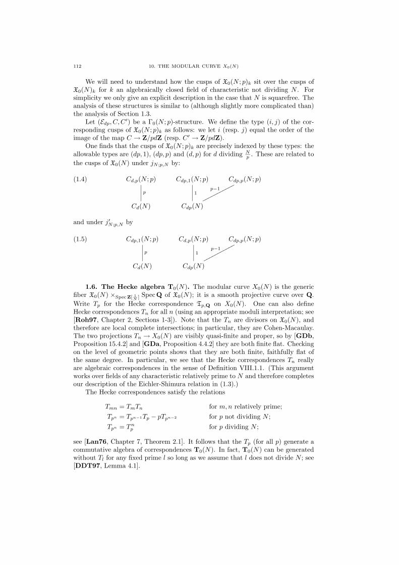
112 10. THE MODULAR CURVE X0(N)
We will need to understand how the cusps of X0(N ; p)k sit over the cusps ofX0(N)k for k an algebraically closed field of characteristic not dividing N . Forsimplicity we only give an explicit description in the case that N is squarefree. Theanalysis of these structures is similar to (although slightly more complicated than)the analysis of Section 1.3.
Let (Edp, C, C ′) be a Γ0(N ; p)-structure. We define the type (i, j) of the cor-responding cusps of X0(N ; p)k as follows: we let i (resp. j) equal the order of theimage of the map C → Z/pdZ (resp. C ′ → Z/pdZ).
One finds that the cusps of X0(N ; p)k are precisely indexed by these types: theallowable types are (dp, 1), (dp, p) and (d, p) for d dividing N
p . These are related tothe cusps of X0(N) under jN ;p,N by:
(1.4) Cd,p(N ; p)
p
Cdp,1(N ; p)
1
Cdp,p(N ; p)p−1
ooooooooooo
Cd(N) Cdp(N)
and under j′N ;p,N by
(1.5) Cdp,1(N ; p)
p
Cd,p(N ; p)
1
Cdp,p(N ; p)p−1
ppppppppppp
Cd(N) Cdp(N)
1.6. The Hecke algebra T0(N). The modular curve X0(N) is the genericfiber X0(N) ×Spec Z[ 1
N ] Spec Q of X0(N); it is a smooth projective curve over Q.Write Tp for the Hecke correspondence Tp,Q on X0(N). One can also defineHecke correspondences Tn for all n (using an appropriate moduli interpretation; see[Roh97, Chapter 2, Sections 1-3]). Note that the Tn are divisors on X0(N), andtherefore are local complete intersections; in particular, they are Cohen-Macaulay.The two projections Tn → X0(N) are visibly quasi-finite and proper, so by [GDb,Proposition 15.4.2] and [GDa, Proposition 4.4.2] they are both finite flat. Checkingon the level of geometric points shows that they are both finite, faithfully flat ofthe same degree. In particular, we see that the Hecke correspondences Tn reallyare algebraic correspondences in the sense of Definition VIII.1.1. (This argumentworks over fields of any characteristic relatively prime to N and therefore completesour description of the Eichler-Shimura relation in (1.3).)
The Hecke correspondences satisfy the relations
Tmn = TmTn for m,n relatively prime;Tpn = Tpn−1Tp − pTpn−2 for p not dividing N ;
Tpn = Tnp for p dividing N ;
see [Lan76, Chapter 7, Theorem 2.1]. It follows that the Tp (for all p) generate acommutative algebra of correspondences T0(N). In fact, T0(N) can be generatedwithout Tl for any fixed prime l so long as we assume that l does not divide N ; see[DDT97, Lemma 4.1].

2. THE MODULAR UNIT ∆ 113
1.7. Poincare duality. Fix a prime l ≥ 7 and not dividing N and let V =H1(X0(N)Q,Zl); we wish to fit V into the general framework of Section VIII.8.It follows from the formulas in [MW84, p. 236] and the fact that the diamondautomorphisms act trivially on V that the Hecke operators Tp for p not dividingN are self-adjoint acting on V . However, here we must make the unfortunateassumption that all Tp are self-adjoint acting on V . This is certainly false in general;we make this assumption so that we can proceed in the simpler self-adjoint case. Wewill remove it in the next chapter. Given this, the Poincare pairing ϕ : V ⊗ZlV (1)→Zl is a T0(N)-hermitian, skew-symmetric, Galois equivariant perfect pairing.
1.8. Non-Eisenstein maximal ideals. Let B denote the image of T0(N) inEndZl V ; by self-adjointness this is independent of which map we take. We wishto find a dualizing maximal ideal m of B. There is a very well developed theoryof such ideals; see [DDT97, Chapter 4] and [Til97] for an exposition. The firststep is to find a maximal ideal m of B associated to a newform and such thatthe Galois representation V ⊗B k (where A = Bm and k = A/mA as always) isabsolutely irreducible. This occurs precisely when m is not Eisenstein. (Recall thatm is said to be Eisenstein if Tp ≡ p + 1 (mod m) for all primes p congruent to 1modulo N ; see [DDT97, Section 4.3, esp. Lemma 4.12].) Since l does not divideN , [Til97, Theorem 3.4] and the proofs of its corollaries show that a non-Eisensteinm containing l is dualizing in our sense. In particular, A is Gorenstein. Fix forthe remainder of the chapter one such maximal ideal m and a corresponding choiceof Gorenstein trace tr : A → Zl. Let η ∈ A denote the corresponding congruenceelement.
1.9. The finite/singular structure. Let T = End0AH(1) considered as a
GQ-module. We give T the finite/singular structure as in Section IX.4: that is,it is unramified away from Nl, minimally ramified at N and crystalline at l. Wewill assume below that N is squarefree so that H is ordinary at primes dividing N ;thus the minimally ramified structure will coincide with the weak structure. Wewill return to this below.
2. The modular unit ∆
We assume from now on that N is squarefree. In order to construct a cohesiveFlach system for T as in Chapter IX.6, we first must find an admissible marking forthe algebra T0(N). Following Flach we choose ∆, the unique normalized rationalcusp form of weight 12 and level 1. In fact, we will see that this is essentially theonly choice, at least if we constrain the divisor to the cusps. (We prefer not to evencontemplate non-cuspidal divisors.)
Lemma 2.1. The marking ∆ is admissible for the Hecke algebra T0(N). Fur-thermore, the only cusp forms of any weight (and level dividing N) which yieldadmissible markings for T0(N) are rational multiples of powers of ∆.
Proof. Since one can check if a divisor vanishes after base extension, for thisproof all of the varieties and divisors we consider will be over Q; we will omit thisfrom our notation. On the modular curve X(1), ∆ lies in Ω⊗6
X(1) and has divisorC1(1). It follows easily that on X0(N), ∆ lies in Ω⊗6
X0(N) and has divisor
(2.1)∑d|N
dCd(N).
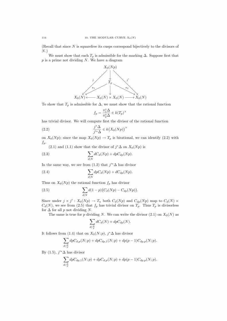
114 10. THE MODULAR CURVE X0(N)
(Recall that since N is squarefree its cusps correspond bijectively to the divisors ofN .)
We must show that each Tp is admissible for the marking ∆. Suppose first thatp is a prime not dividing N . We have a diagram
X0(Np)
j′
???????????????????
j
Tp
π2
''OOOOOOOOOOOOOπ1
wwooooooooooooo
X0(N) X0(N)×X0(N) //oo X0(N)
To show that Tp is admissible for ∆, we must show that the rational function
fp =π∗1∆π∗2∆
∈ k(Tp)×
has trivial divisor. We will compute first the divisor of the rational function
(2.2)j∗∆j′∗∆
∈ k(X0(Np)
)×on X0(Np); since the map X0(Np) → Tp is birational, we can identify (2.2) withfp.
(2.1) and (1.1) show that the divisor of j∗∆ on X0(Np) is
(2.3)∑d|N
dCd(Np) + dpCdp(Np).
In the same way, we see from (1.2) that j′∗∆ has divisor
(2.4)∑d|N
dpCd(Np) + dCdp(Np).
Thus on X0(Np) the rational function fp has divisor
(2.5)∑d|N
d(1− p)(Cd(Np)− Cdp(Np)
).
Since under j × j′ : X0(Np) → Tn both Cd(Np) and Cdp(Np) map to Cd(N) ×Cd(N), we see from (2.5) that fp has trivial divisor on Tp. Thus Tp is divisorlessfor ∆ for all p not dividing N .
The same is true for p dividing N . We can write the divisor (2.1) on X0(N) as∑d|Np
dCd(N) + dpCdp(N).
It follows from (1.4) that on X0(N ; p), j∗∆ has divisor∑d|Np
dpCd,p(N ; p) + dpCdp,1(N ; p) + dp(p− 1)Cdp,p(N ; p).
By (1.5), j′∗∆ has divisor∑d|Np
dpCdp,1(N ; p) + dpCd,p(N ; p) + dp(p− 1)Cdp,p(N ; p).
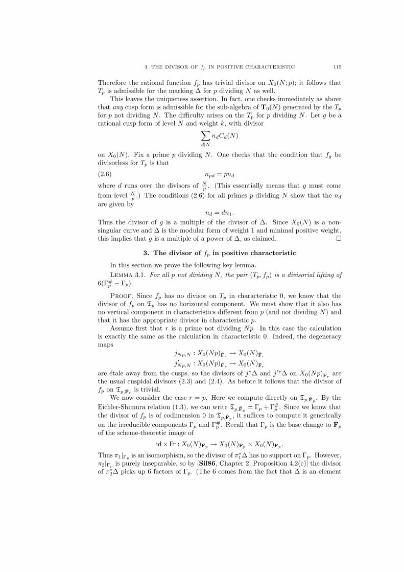
3. THE DIVISOR OF fp IN POSITIVE CHARACTERISTIC 115
Therefore the rational function fp has trivial divisor on X0(N ; p); it follows thatTp is admissible for the marking ∆ for p dividing N as well.
This leaves the uniqueness assertion. In fact, one checks immediately as abovethat any cusp form is admissible for the sub-algebra of T0(N) generated by the Tpfor p not dividing N . The difficulty arises on the Tp for p dividing N . Let g be arational cusp form of level N and weight k, with divisor∑
d|N
ndCd(N)
on X0(N). Fix a prime p dividing N . One checks that the condition that fg bedivisorless for Tp is that
(2.6) npd = pnd
where d runs over the divisors of Np . (This essentially means that g must come
from level Np .) The conditions (2.6) for all primes p dividing N show that the nd
are given bynd = dn1.
Thus the divisor of g is a multiple of the divisor of ∆. Since X0(N) is a non-singular curve and ∆ is the modular form of weight 1 and minimal positive weight,this implies that g is a multiple of a power of ∆, as claimed.
3. The divisor of fp in positive characteristic
In this section we prove the following key lemma.Lemma 3.1. For all p not dividing N , the pair (Tp, fp) is a divisorial lifting of
6(Γ#p − Γp).
Proof. Since fp has no divisor on Tp in characteristic 0, we know that thedivisor of fp on Tp has no horizontal component. We must show that it also hasno vertical component in characteristics different from p (and not dividing N) andthat it has the appropriate divisor in characteristic p.
Assume first that r is a prime not dividing Np. In this case the calculationis exactly the same as the calculation in characteristic 0. Indeed, the degeneracymaps
jNp,N : X0(Np)Fr → X0(N)Fr
j′Np,N : X0(Np)Fr → X0(N)Fr
are etale away from the cusps, so the divisors of j∗∆ and j′∗∆ on X0(Np)Fr arethe usual cuspidal divisors (2.3) and (2.4). As before it follows that the divisor offp on Tp,Fr is trivial.
We now consider the case r = p. Here we compute directly on Tp,Fp . By theEichler-Shimura relation (1.3), we can write Tp,Fp = Γp + Γ#
p . Since we know thatthe divisor of fp is of codimension 0 in Tp,Fp , it suffices to compute it genericallyon the irreducible components Γp and Γ#
p . Recall that Γp is the base change to Fpof the scheme-theoretic image of
id×Fr : X0(N)Fp → X0(N)Fp ×X0(N)Fp .
Thus π1|Γp is an isomorphism, so the divisor of π∗1∆ has no support on Γp. However,π2|Γp is purely inseparable, so by [Sil86, Chapter 2, Proposition 4.2(c)] the divisorof π∗2∆ picks up 6 factors of Γp. (The 6 comes from the fact that ∆ is an element

116 10. THE MODULAR CURVE X0(N)
of Ω⊗6X0(N).) In the same way, the divisor of π∗1∆|Γ#
pis 6Γ#
p , while the divisor ofπ∗2∆|Γ#
pis trivial. Combining these results, we find that fp has divisor 6(Γ#
p − Γp)in characteristic p.
4. The cohesive Flach system
Given our analysis to this point, the proof of the following theorem is notdifficult. Recall that we have assumed that N is squarefree and that l ≥ 7 is aprime not dividing N . B is the image of T0(N) in EndZl H
1(X0(N)Q,Zl) wherewe have assumed that all Tp are self-adjoint. We have A = Bm and
H = H1(X0(N)Q,Zl
)m
for m a non-Eisenstein maximal ideal of B associated to a newform. and we havefixed a Gorenstein trace tr : A→ Zl with congruence element η.
Theorem 4.1. Let H be a modular Galois representation as above and setT = End0
AH(1). Assume that T ⊗A k is absolutely irreducible and that
H1(Q(T ∗[a])/Q, T ∗[a]) = 0
for all ideals a of finite index in A. Then T admits a cohesive Flach system ofEichler-Shimura type of depth η and weight −12 for the structure Sc.
Proof. This is an immediate consequence of Theorem IX.6.1 and Lemma 3.1once we check that the hypotheses of Theorem IX.6.1 are satisfied. X0(N) is co-homologically torsion-free at l since it is a curve. The fact that T ∗p is the trace ofFrp on H is [DDT97, Theorem 3.1] (taking into account that the representationthere is the dual of ours and Frobenius there is arithmetic). This leaves the fournumbered conditions of Section IX.4. By [DDT97, Lemma 3.27], H is minimallyramified and ordinary; Lemma I.5.2 now gives condition 1 since l ≥ 7. That H⊗Akis absolutely irreducible follows from the fact that m is non-Eisenstein, as discussedin Section 1.8; the rest of condition 2 is one of our hypotheses. Condition 3 is aswell, and condition 4 is shown in [DDT97, Lemma 4.1]. Finally, the crystallineconditions come from Proposition VII.10.1 on checking that the cycle class of Tpvanishes in End0
AH; that is, that it is a scalar. This is clear from the computationsof Lemma IX.4.1 and the compatibility of the cycle class map with specializationas in [GBI71, Appendix to Expose 10]. (The singularities of the Hecke correspon-dences are all ordinary double points, which can indeed be resolved over Zl.) Thiscompletes the proof.
Note that the cohesive Flach system of Theorem 4.1 is canonically determinedup to the choice of Gorenstein trace tr. Note also that the depth η is canonicallydetermined as the congruence element of tr.

CHAPTER 11
The modular curve X1(N)
In this chapter we construct cohesive Flach systems of Eichler-Shimura typefor Galois representations associated to modular forms of weight 2 and arbitrarycharacter. We assume for this chapter that N is a squarefree integer greater thanor equal to 7.
1. The geometry of X1(N)
1.1. The model X1(N). Let E/S be a generalized elliptic curve over a Z[ 1N ]-
scheme S. We define a Γ1(N)-structure on E/S to be a section P : Z/NZ → E ofexact order N on fibers; we further require that the subgroup generated by P meetevery irreducible component of fibers which are Neron polygons. (As before thisimplies that only Neron d-gons for d dividing N can support Γ1(N)-structures.) Weconsider two Γ1(N)-structures (E/S, P ) and (E′/S, P ′) to be isomorphic if there isan isomorphism E
'−→ E′ taking P to P ′.The functor from the category of Z[ 1
N ]-schemes to sets sending a scheme S to theset of isomorphism classes of Γ1(N)-structures on generalized elliptic curves over Sis representable (only coarsely representable for N ≤ 4) by a scheme X1(N). X1(N)is a proper, smooth, geometrically connected Z[ 1
N ]-scheme of relative dimension 1.X1(N) admits a proper, regular model over Z as well; see [DI95, Sections 8.2, 8.3,9.2, 9.3].
1.2. The degeneracy maps. For all N dividing M , there is a natural degen-eracy map
jM,N : X1(M)→ X1(N);
here we are using a model for X1(M) defined over Z[ 1N ]. This map is defined on
the moduli level by sending the Γ1(M)-structure (E/S, P ) to the Γ1(N)-structure(E/S, MN P ).
1.3. The diamond automorphisms. For d ∈ (Z/NZ)× there is an automor-phism of the above moduli problem sending a pair (E/S, P ) to the pair (E/S, dP );the corresponding automorphism of X1(N) is called a diamond automorphism andis written 〈d〉. Note that 〈−1〉 acts trivially on X1(N), and that (Z/NZ)×/±1 actsfreely on X1(N).
X0(N) is defined to be the quotient of X1(N) by (Z/NZ)×/ ± 1; the naturalquotient map
πN : X1(N)→ X0(N)
realizes X1(N) as a finite Galois covering of X0(N), of degree φ(N)/2.
117

118 11. THE MODULAR CURVE X1(N)
1.4. The cusps. The closed subschemes of X1(N) corresponding to familiescontaining Neron polygons are called the cusps. The map πN is a finite Galoiscovering unramified at the cusps, so over any algebraically closed field k there areexactly φ(N)/2 cusps of X1(N) sitting over each cusp of X0(N).
1.5. The Hecke correspondences. Fix a prime p not dividing N . Let E/Sbe a generalized elliptic curve over a Z[ 1
N ]-scheme S. We define a Γ1(N ; p)-structureon E/S to be a pair of a Γ1(N)-structure P and a finite flat subgroup scheme Cof E with all geometric fibers of rank p; we require that the group generated by Pand C meet every irreducible component of Neron polygon fibers. The Γ1(N ; p)-moduli problem is representable by a proper, regular, geometrically irreducibleZ[ 1
N ]-scheme X1(N ; p) of relative dimension 1; it becomes smooth over Z[ 1Np ]. (See
[DI95, Sections 8.3 and 9.3].)X1(N ; p) admits two natural degeneracy maps
jN ;p,N : X1(N ; p)→ X1(N)
j′N ;p,N : X1(N ; p)→ X1(N).
jN ;p,N sends the triple (E/S, P,C) to the pair (E/S, P ), and j′N ;p,N sends it to((E/C)/S, P ). These maps are both generically etale away from characteristic p.
We define the pth Hecke correspondence Tp to be the scheme-theoretic imageof the map
jN ;p,N × j′N ;p,N : X1(N ; p)→ X1(N)×Spec Z[ 1N ] X1(N).
Tp is birational to X1(N ; p) away from characteristic p, and has pure codimension1 in X1(N)×Spec Z[ 1
N ] X1(N).We can give a precise description of the closed subscheme Tp,Fp of the proper
smooth variety X1(N)Fp ×Spec Fp X1(N)Fp . We will see later that Tp,Fp can beconsidered as an algebraic self-correspondence on X1(N)Fp ; the Eichler-Shimurarelation states that
Tp,Fp = Γp + Γ′pwhere Γp is the graph of the Frobenius morphism on X1(N)Fp and Γ′p is its modifiedtranspose given as the image of
Fr×〈p〉 : X1(N)Fp → X1(N)Fp × X1(N)Fp .
See [Gro90, p. 454] and [DI95, Section 8.4].
1.6. The Atkin correspondences. Fix a prime p dividing N . Let E/S bea generalized elliptic curve over a Z[ 1
N ]-scheme S. We define a Γ1(N ; p)-structureon E/S to be a pair of a Γ1(N)-structure P and a finite flat subgroup scheme Cof E with all geometric fibers of rank p; we require that the group generated by Pand C meet every irreducible component of Neron polygon fibers and we furtherrequire that C has trivial intersection with the group generated by P . The Γ1(N ; p)-moduli problem is representable by a proper, regular Z[ 1
N ]-scheme X1(N ; p) withgeometrically irreducible fibers and of relative dimension 1; it becomes smooth overZ[ 1
Np ]. See [Gro90, p. 454].X1(N ; p) admits two natural degeneracy maps jN ;p,N and j′N ;p,N to X1(N):
the first sends the triple (E/S, P,C) to the pair (E/S, P ) and the second sends(E/S, P,C) to ((E/C)/S, P ); here P denotes the induced section of E/C, which

1. THE GEOMETRY OF X1(N) 119
still had order N since C is not contained in the group generated by P . We definethe pth Atkin correspondence Tp to be the scheme-theoretic image of the map
jN ;p,N × j′N ;p,N : X1(N ; p)→ X1(N)×Spec Z[ 1N ] X1(N).
As before, Tp is birational to X1(N ; p) away from characteristic p and has purecodimension 1 in X1(N) ×Spec Z[ 1
N ] X1(N). See [MW84, Section 5.5] for moredetails.
There is a natural projection π′N : X1(N ; p) → X0(N ; p); in fact, it is simplythe quotient map by the diamond automorphisms (acting on the point of order N)and is a Galois covering of degree φ(N)/2. It is unramified at the cusps, so it allowsus to understand the cusps on X1(N ; p) in terms of the cusps of X0(N ; p).
1.7. The Hecke algebra T1(N). The modular curve X1(N) is the genericfiber X1(N)×Spec Z[ 1
N ] Spec Q of X1(N); it is a smooth projective curve over Q. Weregard the diamond automorphisms 〈d〉 as algebraic correspondences on X1(N) viatheir graphs. Write Tp for the Hecke correspondence Tp,Q on X1(N). One can alsodefine Hecke correspondences Tn for all n as with X0(N). The same argument asin the X0(N) case shows that these are all algebraic correspondences in our sense.Note also that the compositions 〈d〉 Tn and Tn 〈d〉 are trivially defined since 〈d〉is an automorphism.
The Hecke correspondences satisfy the relations
Tmn = TmTn for m,n relatively prime;
Tpn = Tpn−1Tp − p 〈p〉Tpn−2 for p not dividing N ;
Tpn = Tnp for p dividing N ;
see [Lan76, Chapter 7, Theorem 2.1]. The Tp and diamond automorphisms gen-erate a commutative algebra of correspondences which we denote T1(N). We canomit any Tl from the set of generators of T1(N) so long as l does not divide N by[DDT97, Lemma 4.1].
1.8. The involution wζ. We will need one “exotic” involution of X1(N)Q.Fix a primitive N th root of unity ζ and for every elliptic curve E/S over a Z[ 1
N ]-scheme S, let e : E[N ]×E[N ]→ µN be the scheme-theoretic Weil pairing. wζ is theautomorphism of X1(N)Z[1/N,ζ] sending a pair (E/S, P ) to the pair ((E/C)/S,Q),where C is the subgroup of E generated by P and Q is the unique point of E[N ]such that e(Q,P ) = ζ; see [MW84, Section 5.2] for more details.
Consider now the corresponding involution of X1(N)Q, which we also writeas wζ . wζ is self-adjoint in the sense that w∗ζ = wζ∗ acting on cohomology. wζinteracts with elements of T1(N) via the relation α∗w∗ζ = w∗ζα∗. Since wζ is aninvolution, this implies also that α∗w∗ζ = w∗ζα
∗; see [Til97].We also have a simple interaction with the Galois action on etale cohomology:
for v ∈ H1(X1(N)Q,Zl) and σ ∈ GQ, we have (considering w∗ζ as an involution oncohomology)
σ(w∗ζv) = (σw∗ζ )(σv) = 〈σ〉∗ −1w∗ζ (σv).
Here we are using the natural identification of Gal(Q(ζN )+/Q) with (Z/NZ)×/±1to regard 〈·〉 as a character of GQ. See [MT73, Section 2] for details.

120 11. THE MODULAR CURVE X1(N)
1.9. Poincare duality. Fix a prime l ≥ 7 and not dividing N and let V bethe etale cohomology group H1(X1(N)Q,Zl). The algebra T1(N) is not self-adjointwith respect to the Poincare pairing ϕ : V ⊗Zl V (1)→ Zl. Since wζ is self-adjoint,ϕ does satisfy ϕ(w∗ζ t, t
′) = ϕ(t, w∗ζ t′).
Let B∗ and B∗ be the images of T1(N) in EndZl V , as usual. We define anuntwisting of T1(N) as follows: let B be a free B∗-module of rank 1 (with a chosengenerator ξ) with a B∗-linear action of GQ given by
σξ = 〈σ〉∗ ξ.
We claim that the mapξ ⊗ w∗ζ : V → B ⊗B∗ V
sending v to ξ ⊗ w∗ζv is Galois equivariant. Indeed,
σ(ξ ⊗ w∗ζ (v)
)= σξ ⊗ σ
(w∗ζ (v)
)= 〈σ〉∗ ξ ⊗ 〈σ〉∗ −1w∗ζ (σv)
= ξ ⊗ w∗ζ (σv)
= (ξ ⊗ w∗ζ )(σv).
Thus the triple (w∗ζ , B, ξ) is an untwisting of V .
1.10. Non-Eisenstein maximal ideals. The theory of maximal ideals inT1(N) is very similar to that of T0(N) in Section X.1.8; see [DDT97, Chapter 4]and [Til97, Theorem 3.4]. Let m be a non-Eisenstein maximal ideal ofB∗ associatedto a newform at level N . Set A = B∗m, k = A/mA, H = V ⊗B∗A and A = B⊗B∗A.H ⊗A k is absolutely irreducible as a GQ-module, and as usual we know that A isGorenstein. Fix a choice of Gorenstein trace tr : A→ Zl with congruence elementη. We set T = End0
AH and we endow T with the finite/singular structure which isunramified away from Nl, minimally ramified at N and crystalline at l.
2. Admissible markings
We once again will use ∆ as our admissible marking.Lemma 2.1. The marking ∆ is admissible for the Hecke algebra T1(N).
Proof. Since the maps X1(N ; p) → X0(N ; p) are finite Galois coverings un-ramified at the cusps, the verification that ∆ is divisorless for all Tp follows im-mediately from Lemma X.2.1. It remains to check that ∆ is divisorless for thediamond automorphisms 〈d〉. The induced rational function on the correspondence〈d〉 (which is isomorphic to X1(N)) is simply ∆ 〈d〉 /∆; since ∆ has trivial char-acter, this is the constant 1. Thus 〈d〉 is divisorless for ∆, and we conclude that allof T1(N) is divisorless for ∆.
Let fp denote the rational function on Tp induced by ∆. The calculation of thedivisor of fp in positive characteristic is entirely similar to that of Lemma X.3.1,taking into account the modification in the Eichler-Shimura relation and the factthat 〈p〉 is etale. One finds the following result; here Γp is the graph of Frobeniusand Γ′p is its modified transpose as in Section 1.5.
Lemma 2.2. For all p not dividing N , the pair (Tp, fp) is a divisorial lifting of6(Γ′p − Γp).

3. THE COHESIVE FLACH SYSTEM 121
3. The cohesive Flach system
Recall that we have assumed that N ≥ 5 is squarefree and that l ≥ 7 is a primenot dividing N . B∗ is the image of T1(N) in EndZl H
1(X1(N)Q,Zl). We haveA = B∗m and
H = H1(X0(N)Q,Zl
)m
for m a non-Eisenstein maximal ideal of B∗ associated to a newform, and we havefixed a Gorenstein trace tr : A→ Zl with congruence element η.
Theorem 3.1. Let H be a modular Galois representation as above and setT = End0
AH(1). Assume that T ⊗A k is absolutely irreducible and that
H1(Q(T ∗[a])/Q, T ∗[a]
)= 0
for all ideals a of finite index in A. Then T admits a cohesive Flach system ofEichler-Shimura type of depth η and weight −12.
Proof. The fact that the diamond automorphisms are diamond operators inthe sense of Definition IX.5.1 follows from [DDT97, Theorem 3.1]. The rest of theproof is virtually identical to the proof of Theorem X.4.1. The one complicationis the check that the minimally ramified structure agrees with the weak structure.For this one uses [Car86, Theoreme A] to see that H is either ordinary or elsea direct sum of an unramified character and a tamely ramified character. Thefirst case is dealt with via Lemma I.5.2, while the second case is a straightforwardcomputation.


CHAPTER 12
Kuga-Sato varieties
In this chapter we extend the methods of the previous two chapters to constructcohesive Flach systems of Eichler-Shimura type for modular Galois representationsof higher weight. There are many possible approaches to this. We choose theleast elegant but simplest geometrically: we realize these representations in thecohomology of an “open” Kuga-Sato variety. This requires some modifications ofthe results of Chapters VII and VIII, but has the advantage of not involving anyresolution of singularities.
1. The geometry of Kuga-Sato varieties
1.1. The universal elliptic curve. Recall that X1(N) represents the Γ1(N)-moduli problem for Z[ 1
N ]-schemes. We will be interested only in the complementY1(N) of the cusps in X1(N); Y1(N) is a smooth separated Z[ 1
N ]-scheme, but itis not proper. Y1(N) represents the Γ1(N)-moduli problem for elliptic curves overZ[ 1
N ]; in particular, there exists a universal elliptic curve (with a point of exactorder N) E1(N) over Y1(N).
1.2. Open Kuga-Sato schemes. For k ≥ 0, we let Ek1 (N) denote the k-foldfiber product of E1(N) over Y1(N):
Ek1 (N) =
k︷ ︸︸ ︷E1(N)×Y1(N) E1(N)× · · · ×Y1(N) E1(N) .
Ek1 (N) → Z[ 1N ] is smooth and separated of relative dimension k + 1, but is not
proper. We call Ek1 (N) the open Kuga-Sato scheme of weight k + 2. Ek1 (N) hasa canonical compactification in each characteristic (see [Del71, Lemma 5.4] and[Con, Theorem 4.3.1.1]) but (with one exception) we will not need this.
1.3. The Hecke algebra. For d ∈ (Z/NZ)× there is an automorphism 〈d〉 ofE1(N) sitting over the automorphism 〈d〉 of Y1(N); see [Con, Section 4.2.7] whereit is denoted Id. This in turn yields an automorphism of Ek1 (N) which we denote by〈d〉(k). Similarly, the Hecke correspondences Tp (for all p not dividing N) on Y1(N)yield (by base change) Hecke correspondences T
(k)p on Ek1 (N). (One can also obtain
these operators by a generalization of the methods of Section XI.1.5; see [Sch90,Section 4].)
We define Ek1 (N) to be the generic fiber of Ek1 (N); it is a smooth separatedvariety of dimension k+ 1 over Q. Let T (k)
p denote the Hecke correspondence T(k)p,Q
on Ek1 (N). We note that the projections T (k)p,Q → Ek1 (N) are finite flat of the same
degree (by base change), although T(k)p,Q is not technically an algebraic correspon-
dence in the sense of Chapter VIII as Ek1 (N) is not proper over Q. However, T (k)p
123

124 12. KUGA-SATO VARIETIES
still yields maps in K-theory and the notion of composition as in Section VIII.3is still valid in this setting. In particular, it follows from the relations of [Lan76,Chapter 7, Theorem 2.1] that the T (k)
p and 〈d〉(k) generate a commutative algebra ofcorrespondences for the open variety Ek1 (N); we denote this algebra by T1(N)(k).(Note that we have not yet defined any maps on etale cohomology associated tothese correspondences.) As always we can omit any T
(k)l from the generators of
T1(N)(k) so long as l does not divide N .Let p be a prime not dividing N . For such a p we have the usual Eichler-
Shimura relation for Tp,Fp , regarded as an algebraic correspondence on the smoothvariety Ek1 (N)Fp ×Spec Fp Ek1 (N)Fp :
(1.1) Tp,Fp = Γp + Γ′p
where Γp is the graph of the Frobenius morphism on Ek1 (N)Fp and Γ′p is its modifiedtranspose given as the image of
Fr×〈p〉 : Ek1 (N)Fp → Ek1 (N)Fp ×Spec Fp Ek1 (N)Fp .
See [Con, Theorem 5.3.3.1] for details.
1.4. Untwistings. Let ζ denote a fixed primitive N th root of unity. By [Con,Section 4.2.7], the involution wζ of Y1(N)Z[1/N,ζ] lifts to an involution wζ (called ϕζin [Con]) of E1(N)Z[1/N,ζ]; this in turn yields an involution w
(k)ζ of Ek1 (N)Z[1/N,ζ].
1.5. Galois representations. The production of Galois representations fromV and maximal ideals of B∗ is due to Deligne; see [Del71]. We follow the presen-tation of [Con] via the integral theory of [FJ95].
Fix a prime l ≥ max7, k + 1 not dividing N . We consider first the image
V = H1(Y1(N)Q,Symk R1f∗Zl
)of the map
H1c
(Y1(N)Q,Symk R1f∗Zl
)→ H1
(Y1(N)Q,Symk R1f∗Zl
)of compactly supported cohomology into ordinary cohomology. Here f : E1(N)Q →Y1(N)Q is the structure map. By [Con, Section 5.4], [Sch90, Proposition 4.1.1]and [Car94] (which discusses the integral structure), V is a subquotient of theetale cohomology group Hk+1(Ek1 (N)Q,Zl). We must assume that:
• Ek1 (N) is cohomologically torsion-free at l;• V is a direct summand of Hk+1(Ek1 (N)Q,Zl) as a Zl-module.
Both conditions hold for almost all l.Given these assumptions, we claim that we can apply the methods of Chapters
VII and VIII for the open variety Ek1 (N) ×Spec Q Ek1 (N) to the direct summand(via the above assumptions and the Kunneth formula) EndZl V inside of
(1.2) V0 = H2k+2(Ek1 (N)Q ×Spec Q Ek1 (N)Q,Zl
).
To show this we must consider where proper hypotheses were used in these chapters.Properness was used in three places in Chapter VII. In Section VII.3 it was used toguarantee the local constancy of a higher direct image for an application of purity;however, [Ras89, Lemma 2.1] applies even without this, so that here propernesswas not required. The critical application of properness was in Section VII.7 whereit was used to relate the cohomology of the generic fiber with the cohomology of

2. ADMISSIBLE MARKINGS 125
the special fiber. By [Con, Theorem 5.2.8.1], our V is compatible with such basechange, and one sees immediately that this compatibility is compatible with theinclusion of V into Hk+1(Ek1 (N)Q,Zl). This is sufficient to extend Theorem VII.1.1to apply to EndZl V inside of (1.2); that is, there is a commutative diagram(1.3)
Ek+1,−k−22
(Ek1 (N)× Ek1 (N)
) divFp//
σk+1
Ak+1(Ek1 (N)Fp × Ek1 (N)Fp
)s
H1(Q, V0)
H2k+2(Ek1 (N)Fp × E
k1 (N)Fp ,Zl(k + 1)
)GFp
'
H1(Q,EndZl V )
(EndZl)GFp
H1(Qp,EndZl V ) // H1s (Qp,EndZl V )
for each p not dividing Nl.The last application of properness in Chapter VII occurred in Section 10 where
it was assumed of the ambient variety. However, the deRham cases of these resultsremain valid without this properness, and in our particular case the crystallinecase remains valid by the explicit compactification of Ek1 (N) given by Kuga-Satovarieties.
In Chapter VIII properness was used frequently, but always to insure thatappropriate operations in etale cohomology (covariant functoriality, Poincare du-ality and Kunneth projections) operate entirely on ordinary cohomology (that is,without introducing compact cohomology). The results of [Con, Section 5.2.1.1],[Sch90, Proposition 4.1.1] and especially [FJ95, Theorem 2.1] show that these op-erations for the Hecke algebra T1(N)(k) can be regarded as operating entirely onV . We conclude that the results of Chapter VIII, and thus the results of ChapterIX, remain valid for the Flach map
Ek+1,−k−22
(Ek1 (N)×Spec Q Ek1 (N)
)→ H1(Q,EndZl V )
of (1.3).We let B∗ and B∗ denote the images of T1(N)(k) in EndZl V . We define an
untwisting of V via w(k)ζ exactly as in Section XI.1.9, using [FJ95] to check that
it is an untwisting. Let m be a non-Eisenstein maximal ideal of B∗ associated toa newform; by [FJ95, Theorem 2.1 and Theorem 3.38], such an m is dualizing. Inparticular, H = Vm is free of rank 2 over the Gorenstein ring A = B∗m and H ⊗A kis absolutely irreducible. We fix a choice of Gorenstein trace tr : A → Zl and letη ∈ A be the associated congruence element. We set T = End0
AH(1) and give itthe finite/singular structure which is unramified away from Nl, minimally ramifiedat N and crystalline at l.
2. Admissible markings
Note that by pullback the modular form ∆ yields a differential form on Ek1 (N).We use ∆ as a marking for the Hecke algebra T1(N)(k). It is actually possible in

126 12. KUGA-SATO VARIETIES
this setting to use any modular unit as a marking, but we will not pursue this here.
Lemma 2.1. The marking ∆ is admissible for the Hecke algebra T1(N)(k).
Proof. Recall that T (k)p is obtained by pullback from the Hecke correspon-
dence Tp on Y1(N). By the definition of the rational function induced by a marking,we see that the rational function f (k)
p on T (k)p induced by ∆ is precisely the pullback
of the rational function fp on Tp induced by ∆. Since by Lemma XI.2.1 we knowthat fp has trivial divisor on Tp, we see that T (k)
p is divisorless for ∆. The prooffor the diamond automorphisms is entirely similar.
Lemma 2.2. For all p not dividing N , the pair (T (k)p , f
(k)p ) on Ek1 (N)×Ek1 (N)
is a divisorial lifting of the cycle 6(Γ′p − Γp) on Ek1 (N)Fp ×Spec Fp Ek1 (N)Fp .
Proof. The proof of this is identical to the proof of Lemma XI.3.1 using theEichler-Shimura relation (1.1) in this context and regarding ∆ as a differential formon Ek1 (N); see also [Con, Theorem 5.3.3.1].
3. The cohesive Flach system
Recall that we have assumed thatN ≥ 5 is squarefree and that l ≥ max7, k+1is a prime not dividing N . We have also assumed that
• Ek1 (N) is cohomologically torsion-free at l;• V is a direct summand of Hk+1(Ek1 (N)Q,Zl) as a Zl-module.
B∗ is the image of T1(N)(k) in EndZl V for
V = H1(Y1(N)Q,Symk R1f∗Zl
)regarded as a direct summand ofHk+1(Ek1 (N)Q,Zl). We have A = B∗m andH = Vm
for m a non-Eisenstein maximal ideal of B∗ associated to a newform, and we havefixed a Gorenstein trace tr : A→ Zl with congruence element η.
Theorem 3.1. Let H be a modular Galois representation as above and setT = End0
AH(1). Assume that T ⊗A k is absolutely irreducible and that
H1(Q(T ∗[a])/Q, T ∗[a]
)= 0
for all ideals a of finite index in A. Then T admits a cohesive Flach system ofEichler-Shimura type of depth η and weight −12.
Proof. The proof of this is virtually identical to the proof of Theorem XI.3.1.In particular, the crystalline condition again follows from Proposition VII.10.1 sincethe cycle class of Tp is easily seen to be scalar.
4. Applications
As observed in [Fla92], results like Theorem 3.1 can also be used to show thatcertain deformation problems are unobstructed.
Theorem 4.1. Let H and T be as above; in particular, we assume that l doesnot divide N . Let S denote the set of places of Q dividing Nl together with thearchimedean place. Assume that:
• T ⊗A k is absolutely irreducible;• H1
(Q(T ∗[a])/Q, T ∗[a]
)= 0 for all ideal a of finite index in A;

4. APPLICATIONS 127
• η = A;• H0
(Qp,End0
k(H ⊗A k)(1))
= 0 for all p dividing Nl.Then the deformation problem (with fixed determinant) for the residual representa-tion
ρ : GQS→ Autk(H ⊗A k)
is cohomologically unobstructed. In particular, the associated universal deformationring is a power series ring in two variables over W (k).
Proof. This is derived from Theorem 3.1 as in [Fla92, Section 3]; see also[Wes00, Sections 3–5]. We are forced to impose the determinant condition as theShafarevich-Tate group of the determinant of H ⊗A k is difficult to control if Hdoes not have cyclotomic determinant.


Appendix


APPENDIX A
Edge maps of spectral sequences
In this appendix we prove various compatibility results for edge maps of spectralsequences which are used in the text.
1. Notation for filtered complexes
We will use the notation of [Wei94, Chapter 5]; for clarity we review whatwe will need. We work only in the level of generality which we will need for theapplications. Note that we can afford to be a bit carefree, as we already knowthat everything we are looking at is well-defined. We will also ignore all categoricalissues without further comment.
Let C• be a cochain complex supported in non-negative degree. We will writed for the differential on C•. We assume that C• has a filtration F •C•:
· · · ⊆ Fn+1C• ⊆ FnC• ⊆ · · · ⊆ F 1C• ⊆ F 0C• = C•.
We assume that this filtration is canonically bounded: recall that this means thatFn+1Cn = 0 for each n, so that we have filtrations
0 = Fn+1Cn ⊆ FnCn ⊆ · · · ⊆ F 1Cn ⊆ F 0Cn = Cn.
We associate a spectral sequence to this data as follows. For each p, q, r ≥ 0,set
Apqr =c ∈ F pCp+q | d(c) ∈ F p+rCp+q+1
.
Note that from this definition the differential yields a map
(1.1) d : Apqr → Ap+r,q−r+1r .
Set Epq0 = F pCp+q/F p+1Cp+q and let ηpq : F pCp+q → Epq0 be the quotient map.Define
Zpqr = ηpq(Apqr )
Bpqr = ηpq(d(Ap−r+1,q+r−2
r−1 ))
for r ≥ 0. Set Zpq∞ = ∩rZpqr and Bpq∞ = ∪rBpqr . We have inclusions
0 = Bpq0 ⊆ Bpq1 ⊆ · · · ⊆ Bpq∞ ⊆ Zpq∞ ⊆ · · · ⊆ Z
pq1 ⊆ Z
pq0 = Epq0 .
SetEpqr = Zpqr /B
pqr ;
one checks immediately that this agrees with our previous definition for r = 0. Themaps (1.1) above now yield maps
d : Epqr → Ep+r,q−r+1r
and one checks that this yields a spectral sequence
(1.2) Epq0 ⇒ Hp+q(C•).
131

132 A. EDGE MAPS OF SPECTRAL SEQUENCES
Recall that convergence of (1.2) means that for each p, q there is an isomorphism
(1.3) Epq∞∼= F pHp+q/F p+1Hp+q.
One checks immediately that (1.3) is induced by the inclusion
(1.4) Apq∞ → F pCp+q
where Apq∞ is defined to be ∩rApqr .
2. Edge maps
For this section let Epqa ⇒ Hp+q be any first quadrant spectral sequence. Fixp, q ≥ 0, r ≥ a. Define zEpqr to be the elements of Epqr which survive to Epq∞ ; in thecase of a filtered complex, this is just Zpq∞/B
pqr . We obtain the following sequence
of maps:
(2.1) Epqr ← zEpqr Epq∞ ↔ F pHp+q/F p+1Hp+q → Hp+q/F p+1Hp+q Hp+q.
We will say that this spectral sequence has an x-axis edge map at Epqr if zEpqr = Epqrand F p+1Hp+q = 0. (Often we will omit the “x-axis” if it is clear from context.)Under these hypotheses (2.1) becomes
Epqr Epq∞ ↔ F pHp+q → Hp+q;
that is, we obtain a mapEpqr → Hp+q,
which explains the terminology. Note that if there is an x-axis edge map at Epqrthen there is an x-axis edge map at Epqr′ for all r′ ≥ r.
Example 2.1. Suppose that for some p, q, r the spectral sequence satisfies
(2.2) Ep+1,q−1r = Ep+2,q−2
r = · · · = Ep+q,0r = 0
and
(2.3) Ep+r,q−r+1r = Ep+r+1,q−r
r = Ep+r+2,q−r−1r = · · · = Ep+q+1,0
r = 0.
(2.2) implies that the corresponding E∞ terms vanish; this in turn implies that
F p+1Hp+q/F p+2Hp+q = · · · = F p+qHp+q/F p+q+1Hp+q = 0;
thus F p+1Hp+q = 0. (2.3) implies that Epqr = zEpqr since every later differentialfrom the (p, q) entry maps to 0. We conclude that under these conditions there isan x-axis edge map at Epqr .
There is a similar theory for y-axis edge maps: define bEpqr to be the quotientof Epqr by all boundaries which ever map to it; in the case of a filtered complex, itis Zpqr /B
pq∞ . There is a sequence of maps
(2.4) Hp+q ← F pHp+q F pHp+q/F p+1Hp+q ↔ Epq∞ → bEpqr Epqr .
We will say that a spectral sequence has a y-axis edge map at Epqr if bEpqr = Epqrand F pHp+q = Hp+q. Under these conditions (2.4) reduces to
Hp+q F pHp+q/F p+1Hp+q ↔ Epq∞ → Epqr ,
so we obtain a mapHp+q → Epqr .
Again, if there is a y-axis edge map at Epqr , then there is a y-axis edge map at Epqr′for all r′ ≥ r.

3. EDGE MAPS IN SPECTRAL SEQUENCES OF FILTERED COMPLEXES 133
Example 2.2. Suppose that for some p, q, r we have
Ep−1,q+1r = Ep−2,q+2
r = · · · = E0,p+qr = 0
andEp−r,q+r−1r = Ep−r−1,q+r
r = Ep−r−2,q+r+1r = · · · = E0,p+q+1
r = 0.Then as in Example 2.1 one shows that there is a y-axis edge map at Epqr .
In the following we will work exclusively with x-axis edge maps, but the proofsall adapt immediately to the y-axis case as well.
3. Edge maps in spectral sequences of filtered complexes
Let C•1 and C•2 be filtered complexes as before. Suppose that we are given amap C•1 → C•2 compatible with the filtrations. This induces a map
Epqr (C•1 )→ Epqr (C•2 )
of spectral sequences and a map
Hp+q(C•1 )→ Hp+q(C•2 )
of cohomology groups.Proposition 3.1. Suppose that for some p, q, r there are edge maps
Epqr (C•1 )→ Hp+q(C•1 );
Epqr (C•2 )→ Hp+q(C•2 ).Then the diagram
Epqr (C•1 ) //
Epqr (C•2 )
Hp+q(C•1 ) // Hp+q(C•2 )
commutes.
Proof. Consider the expanded diagram
(3.1) Epqr (C•1 ) //
Epqr (C•2 )
Epq∞(C•1 ) //
Epq∞(C•2 )
F pHp+q(C•1 )/F p+1Hp+q(C•1 ) //
F pHp+q(C•2 )/F p+1Hp+q(C•2 )
Hp+q(C•1 ) // Hp+q(C•2 )
All maps in (3.1) exist by our assumption that the edge maps exist. The first andlast squares commute by the definitions of morphisms of spectral sequences andfiltered complexes. This leaves the middle square: as we observed in (1.4), themaps
Epq∞(C•i )→ F pHp+q(C•i )/F p+1Hp+q(C•i )

134 A. EDGE MAPS OF SPECTRAL SEQUENCES
are induced by the inclusions Apq∞ → F pCp+q, and now the commutativity of themiddle square is clear as well.
4. Edge maps in Grothendieck spectral sequences I
Let A, B and C be abelian categories such that A and B have enough injectives.Let G : A → B and F : B → C be left exact functors. Suppose that G maps injectiveobjects to F -acyclic objects. Under these hypotheses for each object A of A oneobtains a Grothendieck spectral sequence
(4.1) Epq2 = (RpF )(RqG)(A)⇒ Rp+q(FG)(A).
(4.1) is constructed as follows: one begins with an injective resolution A→ I• of A.The complex G(I•) admits a Cartan-Eilenberg resolution J••. The Grothendieckspectral sequence (4.1) is the spectral sequence associated to the filtration by rowsof the total complex of the double complex F (J••); see [Wei94, Section 5.8] fordetails.
Now let A1 and A2 be two objects of A and write Epqr (A1) and Epqr (A2) for thecorresponding Grothendieck spectral sequences. Suppose that there is a morphismA1 → A2 in A. We now construct a corresponding morphism Epqr (A1)→ Epqr (A2)of spectral sequences. Begin with injective resolutions A1 → I•1 and A2 → I•2 . Stan-dard properties of injective resolutions show that the map A1 → A2 lifts to a mapof complexes I•1 → I•2 . This in turn yields a map of the complexes G(I•1 )→ G(I•2 ),and this lifts to a map J••1 → J••2 of any corresponding Cartan-Eilenberg resolu-tions. Taking F of these complexes and passing to the associated total complexyields a map
(4.2) TotF (J••1 )→ TotF (J••2 )
compatible with filtrations by rows or columns. (4.2) in turn yields a map of theassociated Grothendieck spectral sequences. Proposition 3.1 can be restated in thissituation as follows.
Proposition 4.1. Let A1 → A2 be a morphism in A. This morphism inducesa morphism Epqr (A1) → Epqr (A2) of spectral sequences. Suppose further that forsome p, q, r there are edge maps
Epqr (A1)→ Rp+q(FG)(A1);
Epqr (A2)→ Rp+q(FG)(A2).
Then the diagram
Epqr (A1) //
Epqr (A2)
Rp+q(FG)(A1) // Rp+q(FG)(A2)
commutes.

5. EDGE MAPS IN GROTHENDIECK SPECTRAL SEQUENCES II 135
5. Edge maps in Grothendieck spectral sequences II
Suppose that one is given categories and functors forming a commutative dia-gram
A1G1 //
α
B1F1 //
β
C
A2G2 // B2
F2
??
Suppose that the Fi, Gi are left exact, that Gi maps injectives to Fi-acyclics, andthat α and β are exact. Given an object A of A1, these hypotheses allow us toform Grothendieck spectral sequences Epqr,1 for A and Epqr,2 for αA.
Proposition 5.1. Under the above hypotheses there is a natural map of spectralsequences Epqr,1 → Epqr,2 defined at the r = 0 stage. For r = 2 it agrees with the naturalmap
RpF1RqG1(A)→ RpF2R
qG2(αA).
Furthermore, if for some p, q, r there exist edge maps
Epqr,1 → Rp+q(F1G1)(A);
Epqr,2 → Rp+q(F2G2)(αA);
then the diagram
Epqr,1 //
Epqr,2
Rp+q(F1G1)(A) // Rp+q(F2G2)(αA)
commutes, where the bottom map is the natural map.
Proof. Begin with an injective resolution A → I•1 . Let J••1 be a Cartan-Eilenberg resolution of the complex G1(I•1 ). The Grothendieck spectral sequencefor F1 and G1 is the spectral sequence associated to the filtration by rows of thetotal complex of F1(J••1 ).
The same construction for αA yields an injective resolution I•2 and a Cartan-Eilenberg resolution J••2 of G2(I•2 ). Since α is exact, αI•1 is still exact; thus it is aresolution of αA. This implies that there exists a map of complexes αI•1 → I•2 . Thisyields a map G2αI
•1 → G2I
•2 . Since G2α = βG1, we obtain a map βG1I
•1 → G2I
•2 .
β is exact, so βJ••1 is a resolution of βG1I•1 and thus maps to the Cartan-Eilenberg
resolution J••2 .Applying F2 yields a map F2βJ
••1 → F2J
••2 . Since F2β = F1, this is a map
(5.1) F1J••1 → F2J
••2
of double complexes. (5.1) induces a map of filtered complexes, and the propositionnow follows from Proposition 3.1 so long as we check that the maps Epq2,1 → Epq2,2
and Rp+q(F1G1)(A)→ Rp+q(F2G2)(αA) are the natural maps.We begin with Epq2,1 → Epq2,2. These maps are induced from (5.1) after first
taking horizontal cohomology and then vertical cohomology. By the definition ofa Cartan-Eilenberg resolution, horizontal cohomology of J••i yields resolutions (of

136 A. EDGE MAPS OF SPECTRAL SEQUENCES
complexes) Hq(GiI•)→ Jq•i . By the definition of derived functors, we can identifythese with resolutions
RqG1(A)→ Jq•1
RqG2(αA)→ Jq•2 .
Since the map βJ••1 → J••2 sits over a map βG1I•1 → G2I
•2 , we now see immediately
that the map Epq1,1 → Epq1,2 (which is what we obtain after horizontal cohomology)sits over the natural maps βRqG1(A) → RqG2(αA). The Epq1,i’s form injectiveresolutions of these and the cohomology computes the right derived functors ofthe Fi. Since the map Epq1,1 → Epq1,2 sits over these natural maps we see now thatEpq2,1 → Epq2,2 coincides with the natural maps RpF1R
qG1(A)→ RpF2RqG2(αA), as
claimed.For the naturality of the other maps, it is immediate from the definitions that
the map Rp+qF1(G1I•1 ) → Rp+qF2(G2I
•2 ) induced by the spectral sequence map
Epqr,1 → Epqr,2 is the natural map. We must check that the corresponding mapRp+q(F1G1)(A) → Rp+q(F2G2)(αA) obtained from the collapsing of IEpqr,i is thenatural map. Recall that to compute in this spectral sequence we first take verticalcohomology and then take horizontal cohomology. But since Gi takes injectivesto Fi-acyclics, after taking vertical cohomology (which computes RqFi(GiI•)), weare left with a single row R0Fi(GiI•) = FiGi(I•). One now sees as before thathorizontal cohomology yields the usual map Rp+q(F1G1)(A) → Rp+q(F2G2)(αA).
6. Boundary maps of exact sequences of filtered complexes
Let C• be a filtered complex as in Section 1. Note that in the first stage ofthe spectral sequence constructed from C• the differentials are all horizontal. Thatis, for fixed q, E•q1 can be considered as a complex as well, and its cohomology isnothing other than E•q2 .
Now let0→ C•1 → C•2 → C•3 → 0
be an exact sequence of filtered complexes. Suppose in addition that for some q theinduced sequence
0→ E•q1 (C•1 )→ E•q1 (C•2 )→ E•q1 (C•3 )→ 0
is also exact. We obtain long exact sequences of cohomology in both cases:
(6.1) · · · → Hn−1(C•3 )→ Hn(C•1 )→ Hn(C•2 )→ Hn(C•3 )→ Hn+1(C•1 )→ · · ·
(6.2) · · · → Ep−1,q2 (C•3 )→ Epq2 (C•1 )→ Epq2 (C•2 )→ Epq2 (C•3 )→ Ep+1,q
2 (C•1 )→ · · ·
In particular, we have boundary maps
Hp+q(C•3 )→ Hp+q+1(C•1 )
Epq2 (C•3 )→ Ep+1,q2 (C•1 )
for each p.Proposition 6.1. Suppose that for some p, q ≥ 0 there exist edge maps
Epq2 (C•3 )→ Hp+q(C•3 );
Ep+1,q2 (C•1 )→ Hp+q+1(C•1 ).

7. BOUNDARY MAPS OF GROTHENDIECK SPECTRAL SEQUENCES 137
Then the diagram
(6.3) Epq2 (C•3 ) //
Ep+1,q2 (C•1 )
Hp+q(C•3 ) // Hp+q+1(C•1 )
commutes.
Proof. Consider the diagram (in the notation of Section 1)
(6.4) Ap+1,q1 (C•1 ) // Ap+1,q
1 (C•2 ) // Ap+1,q1 (C•3 )
Apq1 (C•1 ) //
OO
Apq1 (C•2 ) //
OO
Apq1 (C•3 )
OO
On the one hand, (6.4) surjects onto the diagram
Ep+1,q1 (C•1 ) // Ep+1,q
1 (C•2 ) // Ep+1,q1 (C•3 )
Epq1 (C•1 ) //
OO
Epq1 (C•2 ) //
OO
Epq1 (C•3 )
OO
from which the boundary maps of (6.2) are computed. We can therefore alsocompute these boundary maps after lifting to the diagram (6.4). (Recall thatthe boundary map is computed by lifting from Epq1 (C•3 ) to Epq1 (C•2 ), mapping toEp+1,q
1 (C•2 ) and pulling back to Ep+1,q1 (C•1 ).)
On the other hand, (6.4) naturally injects into the diagram
Cp+q+1(C•1 ) // Cp+q+1(C•2 ) // Cp+q+1(C•3 )
Cp+q(C•1 ) //
OO
Cp+q(C•2 ) //
OO
Cp+q(C•3 )
OO
from which one computes the boundary maps of (6.1). The edge maps (when theyexist) are induced by these injections. Since boundary maps are computed by thesame procedure in both cases, it is now clear (6.3) commutes.
7. Boundary maps of Grothendieck spectral sequences
We return now to the set-up of Section 4. We now assume that we have threeleft exact functors
F1, F2, F3 : B → Cand that G : A → B takes injectives to Fi-acyclic objects for each i. Supposefurther that for any injective object I of B, the sequence
(7.1) 0→ F1(I)→ F2(I)→ F3(I)→ 0
is exact.Let us now go through the construction of the Grothendieck spectral sequence
again. Begin with an object A of A. One first forms an injective resolution A→ I•
of A. Next, one takes a Cartan-Eilenberg resolution J•• of the complex G(I•).

138 A. EDGE MAPS OF SPECTRAL SEQUENCES
Applying each Fi to this, we obtain three double complexes Fi(J••) in C. In fact,we obtain an exact sequence
0→ F1(J••)→ F2(J••)→ F3(J••)→ 0
of double complexes by the exactness of (7.1). This in turn yields an exact sequence
0→ TotF1(J••)→ TotF2(J••)→ TotF3(J••)→ 0
of the total complexes, compatible with filtrations by rows and columns.Consider now the filtrations of the Fi(J••) by rows. At the first stage of the
associated spectral sequence one takes the horizontal cohomology. Since J•• isa Cartan-Eilenberg resolution, we can first form the cohomology of the complexJ•• and then apply Fi. By the definition of a Cartan-Eilenberg resolution, thehorizontal cohomology of J•• yields injective resolutions of the cohomology complexH•(G(I•)). The first stage of the spectral sequence is obtained by applying Fi tothis double complex; since the complex still consists of injectives, we again obtainan exact sequence of double complexes
0→ E••1,1 → E••1,2 → E••1,3 → 0
where the spectral sequence E••1,i is the Grothendieck spectral sequence for thecomposition of Fi and G. In particular, we get boundary maps Ep+1,q
2 → Ep,q2 as in(6.2). Given all of this, fixing q and translating Proposition 6.1 into the languageof Grothendieck spectral sequences yields the following result.
Proposition 7.1. Let F1, F2, F3, G be functors as above. Suppose that forsome p, q, r and A there exist edge maps
RpF3RqG(A)→ Rp+q(F3G)(A)
andRp+1F1R
qG(A)→ Rp+q+1(F1G)(A).Then the diagram
RpF3RqG(A) //
Rp+1F1RqG(A)
Rp+q(F3G)(A) // Rp+q+1(F1G)(A)
of edge maps and boundary maps commutes.
8. Edge maps of exact couples
We conclude this appendix by considering the spectral sequence of an exactcouple. Since [Wei94, Section 5.9] does not consider the cohomological case, wefirst set our notation. We will work in a somewhat restricted setting, as this is allwhich we will need for the applications.
We being by recalling the construction of the derived couple. Our terminologyis adapted to our situation and is not standard. Consider an exact diagram E1
Di // D
j~~~~~~~~~
E
k
``@@@@@@@

8. EDGE MAPS OF EXACT COUPLES 139
We define the (second) derived couple E2 to be
i(D) i // i(D)
j(2)xxppppppppppp
ker(jk)/ im(jk)k
ffNNNNNNNNNNN
where j(2)(i(d)) = j(d). One checks easily that these maps are all well defined andthat E2 is an exact couple; see [Wei94, Definition 5.9.1]. The rth derived coupleEr of E1 is defined to be the exact couple obtained from E1 after r− 1 iterations ofthis construction.
Now suppose further that D and E are bigraded: D = ⊕pqDpq, E = ⊕pqEpq.Assume also that the maps i, j and k have bidegrees (−1, 1), (0, 0) and (1, 0)respectively. Let Er be the rth derived couple, and let Epqr be the (p, q)-gradedpiece of the E-term in this couple. Letting j(r)k be the differential for Epqr , onesees immediately that j(r)k has bidegree (r,−r + 1), so that Epqr is a spectralsequence.
We now make some more simplifying assumptions. Assume that E is concen-trated in the first quadrant; that Dpq = 0 for q < p; and that ipq : Dpq → Dp−1,q+1
is an isomorphism for p ≤ 0. In this situation one shows easily that Epqr convergesto Hn = D0,n, with filtration F pHn = ir(Dp,n−p) for any r ≥ p (here using the factthat i is eventually an isomorphism). For any r large enough so that Epqr = Epq∞ ,the isomorphism
(8.1) F pHn/F p+1Hn = ir(Dp,n−p)/ir+1(Dp,n−p) ∼= Epqr = Epq∞
is induced by j(r).Suppose now that we have a morphism (of degree (0, 0)) E1 → E2 of bigraded
exact couples. It is immediate from the construction above that this induces amorphism
Epqr (E1)→ Epqr (E2)
of the corresponding spectral sequences. In the proposition below we consider onlyx-axis edge maps; the y-axis case is somewhat different.
Proposition 8.1. Suppose that for some p, q, r there exist x-axis edge maps
Epqr (E1)→ Hp+q(E1);
Epqr (E2)→ Hp+q(E2).
Then the diagram
Epqr (E1) //
Epqr (E2)
Hp+q(E1) // Hp+q(E2)
commutes, where the bottom map is induced from the map D0,n1 → D0,n
2 .

140 A. EDGE MAPS OF SPECTRAL SEQUENCES
Proof. Consider the diagram
Epqr (E1) //
Epqr (E2)
Epq∞(E1) //
Epq∞(E2)
F pHp+q(E1)/F p+1Hp+q(E1) //
F pHp+q(E2)/F p+1Hp+q(E2)
Hp+q(E1) // Hp+q(E2)
Recalling the definitions of each object, the only non-obvious commutativity is themiddle square, and this is also clear since by (8.1) the maps can be taken to beinduced by j(r) in both cases.

APPENDIX B
Gorenstein linear algebra
In this appendix we will prove the results on linear algebra over Gorensteinrings which we will need in the text. We also include a basic discussion of bilateralderivations and a few results on torsion Zl-modules.
1. Definitions
We will restrict ourselves to the case of finite, flat, local Zl-algebras.Definition 1.1. Let A be a finite, flat, local Zl-algebra with residue field k.
We say that A is Gorenstein if Ext1A(k,A) ∼= k.
Note that HomA(k,A) = 0 since A is torsion-free. Since A necessarily has Krulldimension 1, this implies that this definition is the same (at least for finite, flat,local Zl-algebras) as that of [Mat86, Section 18].
It is a general fact [Mat86, Theorem 21.3] that local complete intersectionrings (and therefore regular local rings) are Gorenstein. In particular, any ring ofthe form Zl[x]/f(x) for a monic polynomial f(x) is Gorenstein. Gorenstein ringsare also necessarily Cohen-Macaulay; see [Mat86, Theorem 18.1].
The following characterization of finite, flat, local, Gorenstein Zl-algebras ismuch more concrete and will be especially useful for us. For a finite, flat, localZl-algebra A, we make HomZl(A,Zl) an A-module via af(x) = f(ax) for a ∈ Aand f ∈ HomZl(A,Zl). Note that HomZl(A,Zl) is isomorphic to A as a Zl-module,but they need not be isomorphic as A-modules.
Lemma 1.2. Let A be a finite, flat, local Zl-algebra with maximal ideal m andresidue field k. Then the following conditions are equivalent.
(1) A is Gorenstein;(2) dimk(A/lA)[m] = 1;(3) HomZl(A,Zl) is free of rank 1 as an A-module.
Proof. To prove the equivalence of the first two statements, consider the exactsequence
(1.1) 0→ Al→ A→ A/lA→ 0.
Since HomA(k,A) = 0, we obtain from (1.1) an exact sequence
(1.2) 0→ HomA(k,A/lA)→ Ext1A(k,A) l→ Ext1
A(k,A).
But l kills k and thus kills Ext1A(k,A); therefore (1.2) yields an isomorphism
HomA(k,A/lA) ∼= Ext1A(k,A).
HomA(k,A/lA) naturally identifies with (A/lA)[m], from which the equivalence of(1) and (2) is clear.
141

142 B. GORENSTEIN LINEAR ALGEBRA
To prove the equivalence of the second two statements, we will first show thatdimk(A/lA)[m] = 1 is equivalent to HomFl(A/lA,Fl) being free of rank 1 overA/lA. First assume that HomFl(A/lA,Fl) is free of rank 1 over A/lA. We have
(1.3) (A/lA)[m] ∼= HomFl(A/lA,Fl)[m] ∼= HomFl(A/m,Fl).
The last term in (1.3) is easily seen to be a k-vector space of dimension 1, so that(A/lA)[m] is as well, as claimed.
Next assume that dimk(A/lA)[m] = 1. We have an isomorphism
(1.4) HomFl(A/lA,Fl)⊗A/lA A/m ∼= HomFl
((A/lA)[m],Fl
).
A/lA[m] is a one-dimensional k-vector space, so HomFl(A/lA,Fl) ⊗A/lA k is aswell. Nakayama’s lemma shows that any lift of a generator of this module toHomFl(A/lA,Fl) will generate it as well; that is, HomFl(A/lA,Fl) is a cyclic A/lA-module. An easy Fl-dimension count together with (1.4) now shows that it mustbe free of rank 1 over A/lA. This establishes the asserted equivalence.
To prove the lemma it now suffices to show that HomFl(A/lA,Fl) ∼= A/lA isequivalent to HomZl(A,Zl) ∼= A. For this, note that
HomZl(A,Zl)⊗A A/lA ∼= HomFl(A/lA,Fl).
From here a Nakayama’s lemma argument and a Zl-rank count finish the proof.
Note that Lemma 1.2 says that Gorenstein Zl-algebras are in some sense thosewhich are self-dual. To the best of my knowledge, this sort of result first appearedin [Maz77, Chapter 2, Section 15].
2. Gorenstein traces and congruence elements
For the next two sections we fix a finite, flat, local, Gorenstein Zl-algebra A.We will call any A-generator of HomZl(A,Zl) a Gorenstein trace for A. Note thatthe choice of a Gorenstein trace is determined up to multiplication by an elementof A×.
Let tr : A → Zl be a choice of Gorenstein trace for A. Consider the ringA ⊗Zl A, which we will always regard as an A-algebra via multiplication on theright factor of A. We have an isomorphism
HomZl(A,Zl)⊗Zl A∼= HomA(A⊗Zl A,A),
so that this module is free of rank 1 over A ⊗Zl A. (In the A ⊗Zl A-action onHomA(A ⊗Zl A,A), the left factor of A must act on the domain, but the rightfactor can act on either the domain or the range by A-linearity.) tr induces anA⊗Zl A-generator Tr = tr⊗1 : A⊗Zl A→ A of HomA(A⊗Zl A,A):
Tr(a⊗ a′) = tr(a)a′.
Let ∆ : A ⊗Zl A → A be the diagonal map. Since Tr is a generator ofHomA(A ⊗Zl A,A), we can write ∆ = ιTr for a unique ι ∈ A ⊗Zl A. We de-fine the congruence element ηtr associated to tr to be ∆(ι). That is, ηtr is theimage of 1 ∈ A under the maps
(2.1) A ∼= HomA(A,A) ∆−→ HomA(A⊗Zl A,A) αTr 7→α−→ A⊗Zl A∆−→ A.
We define the congruence ideal of A to be the A-ideal ηtrA; the next lemma showsthat this ideal is independent of the choice of Gorenstein trace tr.

3. GORENSTEIN DUALITY 143
Lemma 2.1. For any u ∈ A×,
ηu tr = u−1ηtr.
Proof. u tr is also a generator of HomZl(A,Zl), given by u tr(a) = tr(ua). Theassociated generator of HomA(A ⊗Zl A,A) is therefore Tr′ = (u ⊗ 1) Tr. Writing∆ = ιTr, we have ∆ = ι(u−1 ⊗ 1) Tr′. Thus ηu tr = ∆(ι(u−1 ⊗ 1)) = u−1ηtr asclaimed.
For a definition of the congruence ideal for more general rings in a relativesetting, see [Len97]. For us it will be critical to pin down the congruence elementassociated to a given Gorenstein trace, which more general formulations can notdo.
The next result is useful for giving conditions under which there is an exactsequence 0→ A→ A→ A/ηA→ 0.
Lemma 2.2. Let A be a finite, flat, local, Gorenstein Zl-algebra and let η be anycongruence element for A. Then A is reduced if and only if η is a non-zero-divisor.
3. Gorenstein duality
A key property of modules over Gorenstein rings is that it is possible to gobetween A-linear maps to A and Zl-linear maps to Zl, in the sense of the followinglemmas.
Lemma 3.1. Let M be a finitely generated free A-module. Fix a Gorensteintrace tr of A. Then the map f 7→ tr f is an isomorphism
HomA(M,A) ∼= HomZl(M,Zl).
Proof. One immediately reduces to the case where M is free of rank 1, inwhich case this is just the definition of Gorenstein trace.
Lemma 3.2. Let M be a finitely generated A-module. Fix a Gorenstein tracetr of A. Then the map f 7→ tr f is an isomorphism
HomA(M,A⊗Zl Ql/Zl) ∼= HomZl(M,Ql/Zl).
Proof. This follows from Lemma 3.1 on taking a resolution of M by freeA-modules.
Let M be a finitely generated free A-module. By Lemma 3.1 we can associateto a Gorenstein trace tr : A→ Zl an isomorphism
(3.1) HomA(M,A) ∼= HomZl(M,Zl).
We can use (3.1) to define a map
htr : EndZlM → EndAM
as the composition
EndZlM∼= HomZl(M,Zl)⊗Zl M
∼= HomA(M,A)⊗Zl M
HomA(M,A)⊗AM ∼= EndAM.
htr is a fairly remarkable map, as it associates to a Zl-linear endomorphism of M anA-linear endomorphism of M . The description of htr on A-linear endomorphismsof A will be of fundamental importance to us.

144 B. GORENSTEIN LINEAR ALGEBRA
Lemma 3.3. Let M be a finitely generated free A-module. Let tr be a Gorensteintrace for A. Then the endomorphism
EndAM → EndZlMhtr−→ EndAM
of EndAM is multiplication by ηtr.
Proof. As usual, we reduce immediately to the case M = A. Tracing throughthe maps above, we see that we must prove that the identity map in EndZl A mapsto ι under the isomorphisms
(3.2) EndZl A∼= HomZl(A,Zl)⊗Zl A
∼= A⊗Zl A,
where ι ∈ A ⊗Zl A is such that ∆ = ιTr. But this is clear after making theidentification
(3.3) HomZl(A,Zl)⊗Zl A∼= HomA(A⊗Zl A,A)
and observing that the image of the identity map in (3.3) under (3.2) is precisely∆.
4. Gorenstein pairings
The next result again goes back to [Maz77, Chapter 2, Section 15]; it is yetanother relationship between Gorenstein rings and duality. Let A be a finite, flat,local Zl-algebra and let M and N be finitely generated A-modules. We say that apairing
ψ : M ⊗Zl N → Zlis A-hermitian if ψ(am, n) = ψ(m,an) for all a ∈ A, m ∈M , n ∈ N . Equivalently,this means that the natural maps
M → HomZl(N,Zl)
N → HomZl(M,Zl)are maps of A-modules.
Lemma 4.1. Let A be a finite, flat, local Zl-algebra and let H be a free A-moduleof rank 2. Then A is Gorenstein if and only if there exists an A-hermitian perfectpairing
ψ : H ⊗Zl H → Zl.
Proof. First assume that such a ψ exists. Since ψ is perfect, there is aninduced isomorphism
H ∼= HomZl(H,Zl)of A-modules. Let A† denote the A-module Hom(A,Zl); we need to show that A†
is a free A-module of rank 1. But this follows from the isomorphism
A† ⊕A† ∼= HomZl(H,Zl) ∼= H ∼= A⊕Aand the fact that A is flat over Zl.
For the other direction, let tr : A→ Zl be a Gorenstein trace and let x, y be abasis for H. One checks easily that the pairing ψ given by ψ(ax + by, cx + dy) =tr(ad − bc) is perfect, A-hermitian and even skew-symmetric. This completes theproof.
We will call a pairing as in Lemma 4.1 a Gorenstein pairing.The next result give a method of factoring Gorenstein pairings.

5. SKEW-SYMMETRIC GORENSTEIN PAIRINGS 145
Lemma 4.2. Let A be a finite, flat, local, Gorenstein Zl-algebra and let
ψ : H ⊗Zl H → Zl
be a Gorenstein pairing. Let tr : A→ Zl be any Gorenstein trace for A. Then thepairing ψ factors as
H ⊗Zl H H ⊗A Hψ′−→ A
tr−→ Zl
where ψ′ is an A-linear perfect pairing.
Proof. Since ψ is A-hermitian, it factors through some pairing H⊗AH → Zl.Lemma 3.1 shows that this pairing factors through an A-linear pairing ψ′ : H ⊗AH → A, and one checks immediately that ψ′ is perfect.
5. Skew-symmetric Gorenstein pairings
As the proof of Lemma 4.1 indicates, the most natural Gorenstein pairings arethose that are skew-symmetric. In this section we investigate the linear algebraassociated to such a pairing.
Let A be a finite, flat, local Zl-algebra and let H be a free A-module of rank2. Let
ψ : H ⊗Zl H → Zlbe a skew-symmetric Gorenstein pairing. ψ induces a map
(5.1) ∧2AH → Zl,
and it is easily checked that any choice of isomorphism of A with ∧2AH turns (5.1)
into a Gorenstein trace. Equivalently, we have the following lemma.Lemma 5.1. Let A be a finite, flat, local, Gorenstein Zl-algebra and let
ψ : H ⊗Zl H → Zl
be a skew-symmetric Gorenstein pairing. Let x, y be a fixed A-basis of H such thatψ(x, y) = 1. Then the map tr : A → Zl given by tr(a) = ψ(ax, y) is a Gorensteintrace. Furthermore, ψ factors as
H ⊗Zl H H ⊗A Hψ′−→ A
tr−→ Zl
where ψ′ : H ⊗A H → A is the pairing ψ′(ax+ by, cx+ dy) = ad− bc.
Proof. That the map tr is a Gorenstein trace is just the preceding argumentmade explicit. The factorization then follows by an easy computation.
Recall that there are canonical decompositions
(5.2) EndAH ∼= A⊕ End0AH
(5.3) H ⊗A H ∼= ∧2A ⊕ Sym2
AH.
Lemma 5.2. The map
(5.4) EndAH → HomZl(H ⊗A H,Zl)sending f : H → H to the map gf (h ⊗ h′) = ψ(h ⊗ f(h′)) is an isomorphism ofA-modules. Restricting to the direct summands of (5.2) and (5.3) induces isomor-phisms
(5.5) A ∼= HomZl(∧2AH,Zl)
146 B. GORENSTEIN LINEAR ALGEBRA
(5.6) End0AH
∼= HomZl(Sym2AH,Zl).
Proof. Fix a basis x, y of H such that ψ(x, y) = 1. Let tr be the associatedGorenstein trace as in Lemma 4.2, so that ψ(ax+by, cx+dy) = tr(ad−bc). Now letf be an endomorphism of H with matrix
(a bc d
)with respect to x, y. The associated
homomorphismgf : H ⊗Zl H → A
is given by
(5.7) gf (αx+ βy, γx+ δy) = tr(αγc+ αδd− βγa− βδb).
That (5.4) is an isomorphism follows from (5.7) by an easy calculation using abasis for EndAH. The isomorphisms (5.5) and (5.6) also follow immediately onconsidering the cases a = −d and a = d, b = c = 0.
Corollary 5.3. The isomorphism of Lemma 5.2 induces an isomorphism
EndAH ⊗Zl Ql/Zl ∼= HomZl(H ⊗A H,Ql/Zl).
6. Bilateral derivations
In this section we give the basic theory of bilateral derivations as developedin [Maz]. We make no effort to work in any level of generality which we will notneed for our applications. Let A be a commutative Zl-algebra and let M be anA⊗Zl A-module. A bilateral derivation from A to M is a Zl-linear map
D : A →M
such thatD(βα) = (α⊗ 1)D(β) + (1⊗ β)D(α)
for all α, β ∈ A. Note that if the action on M factors through the diagonal map∆ : A⊗Zl A → A, then a bilateral derivation is nothing more than a derivation inthe usual sense.
The fundamental example of a bilateral derivation is the map δ : A → A⊗Zl Agiven by δ(α) = α⊗ 1− 1⊗ α. Note that the image of δ lies in the kernel I of ∆;one can show that δ : A → I is the universal bilateral derivation.
If M is an A⊗Zl A-module, define Mδ by
Mδ =m ∈M | δ(α)m = 0 for all α ∈ A
.
Mδ is canonically an A-module via ∆.
Lemma 6.1. Let D : A → M be a bilateral derivation and let a be an ideal ofA such that 1⊗ a and a⊗ 1 annihilate M . Then the restriction of D to a yields anA-module homomorphism
D : a/a2 →Mδ.
Proof. If β ∈ a, then the definition of a bilateral derivation shows that
(6.1) (α⊗ 1)D(β) = D(βα) = D(αβ) = (1⊗ α)D(β)
for all α ∈ A. Thus D(a) ⊆ Mδ. If also α ∈ a, then (6.1) shows that D(αβ) = 0;thus D(a2) = 0. This proves the lemma.

6. BILATERAL DERIVATIONS 147
Now let A be a finite, flat, local, reduced, Gorenstein Zl-algebra. Fix a Goren-stein trace tr for A and let η be the associated congruence element; η is a non-zerodivisor since A is reduced. Let M and N be free A-modules of finite rank; M⊗ZlNis an A⊗Zl A-module in the obvious way.
Lemma 6.2. There exists a unique A-module isomorphism
ν : (M ⊗Zl N)δ'−→M ⊗A N
fitting into a commutative diagram
(M ⊗Zl N)δ //
ν
M ⊗Zl N
M ⊗A N η// M ⊗A N
Proof. The uniqueness of such a ν is clear. To define ν it suffices to considerthe case M = N = A. Consider the sequence
(6.2) (A⊗Zl A)δ → A⊗Zl A∆−→ A.
Applying HomZl(·,Zl) to (6.2) yields a sequence
(6.3) HomZl(A,Zl)∆−→ HomZl(A⊗Zl A,Zl)
f−→ HomZl
((A⊗Zl A)δ,Zl
).
The trace tr and Tr identify the first two terms with A and A⊗Zl A, respectively.We claim that to define ν it suffices to prove that there is a commutative diagram
(6.4) HomZl(A⊗Zl A,Zl)f// HomZl
((A⊗Zl A)δ,Zl
)
A⊗Zl A
'·Tr
OO
∆ // A
'
OO
Indeed, given (6.4) it follows immediately from (2.1) that (6.3) fits into a commu-tative diagram
HomZl(A,Zl)' // HomZl
((A⊗Zl A)δ,Zl
)
A
'· tr
OO
η// A
'
OO
By duality we conclude that there is an isomorphism ν : (A ⊗Zl A)δ'−→ A such
that
Aν←− (A⊗Zl A)δ → A⊗Zl A
∆−→ A
is multiplication by η, as claimed.It thus suffices to construct (6.4). Note first that for any α ∈ A ⊗Zl A such
that lα ∈ (A⊗Zl A)δ we must have α ∈ (A⊗Zl A)δ. It follows that (A⊗Zl A)δ is aZl-module direct summand of A⊗Zl A and thus that(6.5)HomZl
((A⊗Zl A)δ,Zl
) ∼= HomZl(A⊗Zl A,Zl)/HomZl
(A⊗Zl A/(A⊗Zl A)δ,Zl
).

148 B. GORENSTEIN LINEAR ALGEBRA
There is a commutative diagram
(6.6) HomZl
(A⊗Zl A/(A⊗Zl A)δ,Zl
) // HomZl(A⊗Zl A,Zl)
δ(A)
'·Tr
OO
// A⊗Zl A
' ·Tr
OO
by the definition of δ. The desired diagram (6.4) now arises as the cokernel of (6.6)via (6.5).
Lemma 6.3. Let H be a free A-module of finite rank with an A-linear action ofsome group G. Assume also that every Jordan-Holder constituent of H ⊗Zl H hastrivial G-invariants. Then there is a canonical isomorphism
H1(G,H ⊗Zl H)δ ∼= H1(G, (H ⊗Zl H)δ
).
Proof. This is an easy argument on the level of cocycles; we omit the details.
Note that Lemma 6.3 applies in particular when H⊗Ak is absolutely irreducibleof rank at least 2.
7. Torsion modules
In this section we collect some results on modules over finite, flat, local Zl-algebras. Let A be a such a Zl-algebra, with maximal ideal m and residue field k.If T is an A-module and a is an ideal of A, then we write T [a] for the a-torsion inT :
T [a] =t ∈ T | αt = 0 for all α ∈ a
.
We will need the following simple facts about A-modules.Lemma 7.1. Let α ∈ A be a non-zero divisor. Then α divides some power of l
in A and αA has finite index in A.
Proof. Since A is finite over Zl and α is a non-zero divisor, α necessarilysatisfies some monic linear equation of the form
αn + an−1αn−1 + · · ·+ a1α+ a0 = 0
with ai ∈ Zl and a0 6= 0. Thus α divides a0, which proves the first statement. Sincea0A ⊆ αA and a0A visibly has finite index in A (as A is free of finite rank over Zl),the second statement is now clear as well.
Lemma 7.2. Let T be an A-module and let t be a non-zero element of T annihi-lated by some power of l. Then there exists α ∈ A such that αt 6= 0 and αt ∈ T [m].
Proof. Since t is l-power torsion, there is a largest power ln of l such thatt0 = lnt 6= 0; thus t0 ∈ T [l]. Note that T [l] is a module over the artinian ring A/lA.Let α1, . . . , αm be generators of m in A; they also generate the maximal ideal ofA/lA and are therefore nilpotent in this ring. It follows that some power of α1
annihilates t0; let n1 be the smallest such power, and set t1 = αn1−11 t0. Continuing
in this way, we obtain a non-zero element tm = αt where α = lnαn1−11 · · ·αnm−1
m .This tm is killed by every generator of m, so it is clearly in T [m].
Lemma 7.3. Let T be a Zl-torsion A-module. If T [m] = 0, then T = 0.

7. TORSION MODULES 149
Proof. Suppose that T 6= 0 and let t be a non-zero element of T . ByLemma 7.2 there is some α ∈ A such that αt is non-zero and annihilated by m.Thus T [m] 6= 0, which yields the desired contradiction.


Bibliography
[Art62] Michael Artin, Grothendieck topologies, Lecture notes, Harvard University Department
of Mathematics, Cambridge, Massachusetts, 1962.[AW67] Michael Atiyah and C.T.C. Wall, Cohomology of groups, In Cassels and Frohlich
[CF67], pp. 94–115.
[Bas73] Hyman Bass (ed.), Algebraic K-theory I (Battelle, 1972), Lecture Notes in Mathe-matics, no. 341, Springer-Verlag, 1973.
[BK90] Spencer Bloch and Kazuya Kato, L-functions and Tamagawa numbers of motives, InCartier et al. [CIK+90], pp. 333–400.
[Car86] Henri Carayol, Sur les representations l-adiques associees aux formes modulaires de
Hilbert, Annales Scientifiques de l’Ecole Normale Superieure 19 (1986), 409–468.[Car94] Henri Carayol, Formes modulaires et representations Galoisiennes a valeuers dans
un anneau local complet, Contempory Mathematics, no. 165, American MathematicalSociety, 1994, pp. 213–237.
[Cas67] Ian Cassels, Global fields, In Cassels and Frohlich [CF67], pp. 42–84.
[CF67] Ian Cassels and Jurg Frohlich (eds.), Algebraic number theory (Brighton, 1965), Aca-demic Press, 1967.
[CIK+90] Pierre Cartier, Luc Illusie, Nicholas Katz, Gerard Laumon, Yuri Manin, and Ken Ribet
(eds.), The Grothendieck festschrift II, Birkhauser, 1990.[Con] Brian Conrad, Modular forms, cohomology and the Ramanujan conjecture, Harvard
University, Fall 1999.[CPS75] Edward Cline, Brian Parshall, and Leonard Scott, Cohomology of finite groups of
Lie type I, Institut des Hautes Etudes Scientifiques, Publications Mathematiques 45
(1975), 169–191.[CR00] Brian Conrad and Karl Rubin (eds.), Arithmetic algebraic geometry (Park City, 1999),
IAS/Park City Mathematics Series, no. 3, American Mathematical Society, 2000.[CSS97] Gary Cornell, Joseph Silverman, and Glenn Stevens (eds.), Modular forms and Fer-
mat’s last theorem (Boston Univesity, 1995), Springer-Verlag, 1997.
[CT95] Jean Louis Colliot-Thelene, Birational invariants, purity and the Gersten conjecture,In Jacob and Rosenberg [JR95], pp. 1–64.
[CTHK97] Jean Louis Colliot-Thelene, Raymond Hoobler, and Bruno Kahn, The Bloch-Ogus-Gabber theorem, In Snaith [Sna97], pp. 31–94.
[CY97] John Coates and Shing-Tung Yau (eds.), Elliptic curves, modular forms and Fermat’s
last theorem (Hong Kong, 1993), International Press, 1997.[DDT97] Henri Darmon, Fred Diamond, and Richard Taylor, Fermat’s last theorem, In Coates
and Yau [CY97], pp. 2–140.[Del71] Pierre Deligne, Formes modulaires et reprentations l-adiques, Seminaire Bourbaki 355
(1971), 139–172.
[DI95] Fred Diamond and John Im, Modular forms and modular curves, In Murty [Mur95],pp. 39–133.
[Dic00] Mark Dickinson, A criterion for the existence of a universal deformation ring, InConrad and Rubin [CR00].
[DK73] Pierre Deligne and Willem Kuyk (eds.), Modular functions of one variable II
(Antwerp, 1972), Lecture Notes in Mathematics, no. 349, Springer-Verlag, 1973.[DR73] Pierre Deligne and Michael Rapoport, Schemas de modules de courbes elliptiques, In
Deligne and Kuyk [DK73], pp. 143–316.[dSL97] Bart de Smit and Henrik Lenstra, Explicit construction of universal deformation rings,
In Cornell et al. [CSS97], pp. 313–326.
151
152 BIBLIOGRAPHY
[EM97] David Eisenbud and Barry Mazur, Evolutions, symbolic squares, and Fitting ideals,
Journal fur die Reine und Angewandte Mathematik 488 (1997), 189–201.[Fal89] Gerd Faltings, Crystalline cohomology and p-adic Galois representations, In Igusa
[Igu89], pp. 25–80.
[FI93] Jean-Marc Fontaine and Luc Illusie, p-adic periods: a survey, In Ramanan andBeauville [RB93], pp. 57–93.
[FJ95] Gerd Faltings and Bruce Jordan, Crystalline cohomology and GL(2,Q), Israel Journalof Mathematics 90 (1995), 1–66.
[FK88] Eberhard Freitag and Reinhardt Kiehl, Etale cohomology and the Weil conjecture,Springer-Verlag, Berlin, 1988.
[FL82] Jean-Marc Fontaine and Guy Laffaille, Construction de representations p-adiques,Annales Scientifiques de l’Ecole Normale Superieure 15 (1982), 547–608.
[Fla92] Matthias Flach, A finiteness theorem for the symmetric square of an elliptic curve,
Inventiones Mathematicae 109 (1992), 307–327.
[Fla95] Matthias Flach, Annihilation of Selmer groups for the adjoint representation of amodular form, In Murty [Mur95], pp. 249–265.
[FM87] Jean-Marc Fontaine and William Messing, p-adic periods and p-adic etale cohomology,In Ribet [Rib87], pp. 179–207.
[Fon82] Jean-Marc Fontaine, Sur certains types de representations p-adiques du groupe de
Galois d’un corps local; construction d’un anneau de Barsotti-Tate, Annals of Math-ematics 115 (1982), 529–577.
[Fon94] Jean-Marc Fontaine, Representations p-adique semi-stables, Periodes p-adiques (Bu-res, 1988), Asterique, no. 223, Societe mathematique de France, 1994, pp. 113–184.
[FPR94] Jean-Marc Fontaine and Bernadette Perrin-Riou, Autour des conjectures de Bloch et
Kato: cohomologie galoisienne et valuers de fonctions L, In Jannsen et al. [JKS94],pp. 599–706.
[Fro67] Jurg Frohlich, Local fields, In Cassels and Frohlich [CF67], pp. 1–41.[Ful98] William Fulton, Intersection theory, Springer-Verlag, New York, 1998.
[GAV73] Alexander Grothendieck, Michael Artin, and Jean-Louis Verdier, Theorie des topos et
cohomologie etale des schemas (1963-1964), Lecture Notes in Mathematics, no. 269,270, 305, Springer-Verlag, 1972-73.
[GBI71] Alexander Grothendieck, Pierre Berthelot, and Luc Illusie, Theorie des intersections ettheoreme de Riemann-Roch, Lecture Notes in Mathematics, no. 225, Springer-Verlag,
1971.
[GDa] Alexander Grothendieck and Jean Dieudonne, Etude cohomologique des faisceauxcoherents, Institut des Hautes Etudes Scientifiques, Publications Mathematiques, vol.
11 (1961), vol. 17 (1963).[GDb] Alexander Grothendieck and Jean Dieudonne, Etude local des schemas et des mor-
phismes de schemas, Institut des Hautes Etudes Scientifiques, Publications Mathema-
tiques, vol. 20 (1964), vol. 24 (1965), vol. 28 (1966), vol. 32 (1967).[GDc] Alexander Grothendieck and Jean Dieudonne, Le langage des schemas, Institut des
Hautes Etudes Scientifiques, Publications Mathematiques, vol. 4 (1960).[Gil81] Henri Gillet, Riemann-Roch theorems for higher algebraic K-theory, Advances in
Mathematics 40 (1981), 203–289.
[GK68] Alexander Grothendieck and Nicolaas Kuiper (eds.), Dix exposes sur la cohomolgiedes schemas, North-Holland Publishing Company, Amsterdam, 1968.
[Gou00] Fernando Gouvea, Deformations of Galois representations, In Conrad and Rubin[CR00].
[Gra77] Daniel Grayson, The K-theory of hereditary categories, Journal of Pure and Applied
Algebra 11 (1977), 67–74.[Gro68] Alexander Grothendieck, Le groupe de Brauer III : Exemples et complements, In
Grothendieck and Kuiper [GK68], pp. 88–188.[Gro77] Alexander Grothendieck, Cohomologie l-adique et fonctions L (1965-1966), Lecture
Notes in Mathematics, no. 589, Springer-Verlag, 1977.
[Gro90] Benedict Gross, A tameness criterion for Galois representations associated to modularforms (mod p), Duke Mathematical Journal 61 (1990), 445–517.
[HS53] Gerhard Hochschild and Jean-Pierre Serre, Cohomology of group extensions, Transac-tions of the American Mathematical Society 74 (1953), 110–134.

BIBLIOGRAPHY 153
[Igu89] Jun-Ichi Igusa (ed.), Algebraic analysis, geometry and number theory (Baltimore,
1988), Johns Hopkins University Press, 1989.[IRS90] Yasutaka Ihara, Ken Ribet, and Jean-Pierre Serre (eds.), Galois groups over Q (Berke-
ley, 1990), Mathematical Sciences Research Instistute Publications, no. 16, Springer-
Verlag, 1990.[Jan90] Uwe Jannsen, Mixed motives and algebraic K-theory, Lecture Notes in Mathematics,
no. 1400, Springer-Verlag, New York, 1990.[JKS94] Uwe Jannsen, Steve Kleiman, and Jean-Pierre Serre (eds.), Motives (Seattle, 1991),
Proceedings of Symposia in Pure Mathematics, no. 55, American Mathematical Soci-ety, 1994.
[JR95] William Jacob and Alex Rosenberg (eds.), K-theory and algebraic geometry: connec-tions with quadratic forms and division algebras (Santa Barbara, 1992), Proceedingsof Symposia in Pure Mathematics, no. 58, American Mathematical Society, 1995.
[JS89] J. Jardine and Victor Snaith (eds.), Algebraic K-theory: connections with geometry
and topology (Alberta, 1987), Kluwer Acadeear=, 1989.[Kis] Mark Kisin, Potential semi-stability of p-adic etale cohomology, preprint.
[KM85] Nicholas Katz and Barry Mazur, Arithmetic moduli of elliptic curves, Princeton Uni-versity Press, Princeton, New Jersey, 1985.
[Lan76] Serge Lang, Introduction to modular forms, Springer-Verlag, Berlin, 1976.
[Len97] Henrik Lenstra, Complete intersections and Gorenstein rings, In Coates and Yau[CY97], pp. 248–257.
[Lev98] Marc Levine, Mixed motives, American Mathematical Society, Providence, Rhode Is-land, 1998.
[Mat86] Hideyuki Matsumura, Commutative ring theory, Cambridge University Press, Cam-
bridge, 1986.[Maz] Barry Mazur, Galois deformations and Hecke curves, Harvard University, spring 1994.
[Maz77] Barry Mazur, Modular curves and the Eisenstein ideal, Institut des Hautes EtudesScientifiques, Publications Mathematiques 47 (1977), 33–186.
[Maz90] Barry Mazur, Deforming Galois representations, In Ihara et al. [IRS90], pp. 385–437.
[Maz97] Barry Mazur, An introduction to the deformation theory of Galois representations, InCornell et al. [CSS97], pp. 243–311.
[Mil86] James Milne, Arithmetic duality theorems, Academic Press, Boston, 1986.[MT73] Barry Mazur and John Tate, Points of order 13 on elliptic curves, Inventiones Math-
ematicae 22 (1973), 41–49.
[Mur95] V. Kumar Murty (ed.), Seminar on Fermat’s last theorem, Canadian MathematicalSociety Proceedings, vol. 17, American Mathematical Society, Providence, Rhode Is-
land, 1995.[MW84] Barry Mazur and Andrew Wiles, Class fields of abelian extensions of Q, Inventiones
Mathematicae 76 (1984), 179–330.
[Pie82] Richard Pierce, Associative algebras, Springer-Verlag, New York, 1982.[Qui73] Daniel Quillen, Higher algebraic K-theory I, In Bass [Bas73], pp. 85–147.
[Ras89] Wayne Raskind, Torsion algebraic cycles on varieties over local fields, In Jardine andSnaith [JS89], pp. 343–388.
[RB93] Sundararaman Ramanan and Arnaud Beauville (eds.), Proceedings of the Indo-French
conference on geometry (Bombay, 1989), Hindustan Book Agency, 1993.[Rib87] Ken Ribet (ed.), Current trends in arithmetical algebraic geometry (Arcata, 1985),
Contemporary Mathematics, no. 67, American Mathematical Society, 1987.[Roh97] David Rohrlich, Modular curves, Hecke correspondences and L-functions, In Cornell
et al. [CSS97], pp. 41–100.
[Rub00] Karl Rubin, Euler systems, Princeton University Press, Princeton, New Jersey, 2000.[Sch90] Anthony Scholl, Motives for modular forms, Inventiones Mathematicae 100 (1990),
419–430.[Ser79] Jean-Pierre Serre, Local fields, Springer-Verlag, New York, 1979.
[Ser97] Jean-Pierre Serre, Galois cohomology, Springer-Verlag, Berlin, 1997.
[Sil86] Joseph Silverman, The arithmetic of elliptic curves, Springer-Verlag, New York, 1986.[Sna97] Victor Snaith (ed.), Algebraic K-theory (Toronto, 1996), Fields Insititute Communi-
cations, no. 16, American Mathematical Society, 1997.

154 BIBLIOGRAPHY
[Til97] Jacques Tilouine, Hecke algebras and the Gorenstein property, In Cornell et al.
[CSS97], pp. 327–342.[Was97] Lawrence Washington, Galois cohomology, In Cornell et al. [CSS97], pp. 101–120.[Wei94] Charles Weibel, An introduction to homological algebra, Cambridge University Press,
Cambridge, England, 1994.[Wes00] Tom Weston, An overview of a theorem of Flach, In Conrad and Rubin [CR00].[Wil95] Andrew Wiles, Modular elliptic curves and Fermat’s last theorem, Annals of Mathe-
matics 142 (1995), 443–551.


![Part II | Galois Theorydec41.user.srcf.net/notes/II_M/galois_theory_thm_proof.pdf · Normal and Galois extensions, automorphic groups. Fundamental theorem of Galois theory. [3] Galois](https://static.fdocuments.net/doc/165x107/5f3b019b8ccd1673676b3f72/part-ii-galois-normal-and-galois-extensions-automorphic-groups-fundamental-theorem.jpg)