On Saaty ’s and Koczkodaj ’s inconsistencies ofpairwise comparison matrices1

Bozóki, S. and Rapcsák, T.

Computer and Automation Research Institute,Hungarian Academy of Sciences,

Budapest, Hungary

Abstract

The aim of the paper is to obtain some theoretical and numerical properties ofSaaty ’s and Koczkodaj ’s inconsistencies of pairwise comparison matrices (PRM ).In the case of 3 × 3 PRM, a differentiable one-to-one correspondence is given be-tween Saaty ’s inconsistency ratio and Koczkodaj ’s inconsistency index based onthe elements of PRM. In order to make a comparison of Saaty ’s and Koczkodaj ’sinconsistencies for 4 × 4 pairwise comparison matrices, the average value of themaximal eigenvalues of randomly generated n× n PRM is formulated, the ele-ments aij (i < j) of which were randomly chosen from the ratio scale

1M

,1

M − 1, . . . ,

12, 1, 2, . . . , M − 1,M,

with equal probability 1/(2M−1) and aji is defined as 1/aij . By statistical analysis,the empirical distributions of the maximal eigenvalues of the PRM depending onthe dimension number are obtained. As the dimension number increases, the shapeof distributions gets similar to that of the normal ones. Finally, the inconsistencyof asymmetry is dealt with, showing a different type of inconsistency.

1. Introduction

In multiattribute decision making (MADM ), the aim is to rank a finite number ofalternatives with respect to a finite number of attributes. Tender evaluations, public pro-curement processes, selections of applicants for positions, decisions on the best portfoliosin investments are real-life decision situations in which MADM models can be used.

In solving a multiattribute decision problem, one needs to know the impor-tances or weights of the not equally important attributes and also the evaluationsof the alternatives with respect to the attributes. One technique, often used, is themethod of pairwise comparisons a concept which is more than two hundred years old.Condorcet (1785) and Borda (1781) introduced it for voting problems in the 1780’s byusing only 0 and 1 in the pairwise comparison matrices. In experimental psychology,Thorndike (1920) and Thurstone (1927) used it in the 1920’s. Especially, pairwise com-parisons based on a ratio scale is one of the basic pillars of the Analytic Hierarchy Process(Saaty, 1980).

1This research was supported, in part, by the Hungarian Scientific Research Fund, Grant Nos.OTKA-T043276, T043241 and K60480.

1

Given n objects, e.g., attributes or alternatives, we suppose that the decision maker(s)is (are) able to compare any two of them. In preference modelling, this assumptionis called comparability. For any pairs (i, j), i, j = 1, 2, . . . , n, the decision maker isrequested to tell how many times the i-th object is preferred (or more important) thanthe j-th one, which result is denoted by aij.

By definition,

aij > 0; (1.1)aii = 1; (1.2)

aij =1

aji

, (1.3)

for any pair of indices (i, j), i, j = 1, 2, . . . , n. The name of matricesA = [aij]i,j=1,2,...,n ∈ Rn×n with properties (1.1-1.3) is pairwise comparison matricesor positive reciprocal matrices (PRM ).

A pairwise comparison matrix A is consistent if it satisfies the transitivity property

aijajk = aik (1.4)

for any indices (i, j, k), i, j, k = 1, 2, . . . , n. Otherwise, A is inconsistent. It was shownby Saaty (1980) that a pairwise comparison matrix is consistent if and only if it is ofrank one. When a pairwise comparison matrix A is consistent, the normalized weightscomputed from A are unique. Otherwise, an approximation of A by a consistent matrix(determined by a vector) is needed.

A crucial point of this methodology is to determine the inconsistency of thepairwise comparison matrices. The only widely accepted rule of inconsistency isdue to Saaty (1980), but his definition does not meet some important requirements(see Section 2 ). The aim of the paper is to make some comparison on Saaty ’s andKoczkodaj ’s inconsistencies of pairwise comparison matrices. The two approaches seemto be completely different, because while Saaty ’s inconsistency ratio is an index for thedeparture from randomness, Koczkodaj ’s inconsistency index is related to the departurefrom consistency with the possibility to locate inconsistency.

In Section 2, the question is how to investigate Saaty ’s and Koczkodaj ’s inconsisten-cies. In Section 3, the inconsistency formulas of 3× 3 pairwise comparison matrices arestudied from theoretical and computational points of view. A differentiable one-to-onecorrespondence is given between Saaty ’s and Koczkodaj ’s inconsistencies. In Section 4,by using statistical tools, the average value of the maximal eigenvalues of randomlygenerated n × n PRM is formulated, the elements aij (i < j) of which were randomly

chosen from the ratio scale1

M,

1

M − 1, . . . ,

1

2, 1, 2, . . . ,M − 1,M , with equal probability

1/(2M − 1) and aji is defined as 1/aij. Then, a comparison of Koczkodaj ’s inconsistencyindex and Saaty ’s inconsistency ratio is given for 4× 4 pairwise comparison matrices.In Section 5, the inconsistency of random pairwise comparison matrices is investigatedand by statistical analysis, the empirical distributions of the maximal eigenvalues of thePRM depending on the dimension number are obtained. As the dimension number in-creases, the shape of distributions gets similar to that of the normal ones. In Section 6,the inconsistency of asymmetry is dealt with, showing a different type of inconsistency.

2

2. Inconsistency indices

In real-life decision problems, pairwise comparison matrices are rarely consistent.Nevertheless, decision makers are interested in the level of consistency of the judgements,which somehow expresses the goodness or “harmony” of pairwise comparisons totally,because inconsistent judgements may lead to senseless decisions.

Saaty (1980) proposed the following method for calculating inconsistency. Computingthe largest eigenvalue λmax of A, he has shown that λmax ≥ n and equals to n if andonly if A is consistent. Then, inconsistency index (CIn) is defined by

CIn =λmax − n

n− 1,

which gives the average inconsistency. Mathematically, inconsistency is not but arescaling of the largest eigenvalue. Since λmax ≥ n, CIn is always non-negative. Theinconsistency index in its own has no meaning, unless we compare it with some bench-mark to determine the magnitude of the deviation from consistency. Let a set of e.g., 500random pairwise comparison matrices of size n × n be generated so that each elementaij (i < j) be randomly chosen from the scale

1

9,1

8,1

7, . . . ,

1

2, 1, 2, . . . , 8, 9,

and aji is defined as1

aij

. Let RIn denote the average value of the randomly obtained

inconsistency indices, which depends not only on n but on the method of generatingrandom numbers, too. The inconsistency ratio (CRn) of a given pairwise comparisonmatrix A indicating inconsistency is defined by

CRn =CIn

RIn

.

If the matrix is consistent, then λmax = n, so CIn = 0 and CRn = 0, as well.Saaty concluded that an inconsistency ratio of about 10% or less may be consideredacceptable. The intuitive meaning of the 10 percent rule is skipped by several authors.A statistical interpretation of the 10 percent rule is given by Vargas (1982). Morerecently, Saaty ’s threshold is 5% for 3× 3, and 8% for 4× 4 matrices (Saaty, 1994).

It is emphasized that the inconsistency ratio CRn is related to Saaty ’s scale. Thestructuring process in AHP specifies that items to be compared should be within one or-der of magnitude. This helps avoid inaccuracy associated with cognitive overload as wellas aijajk relationships that are beyond the 1-9 scale, see e.g. Lane and Verdini (1989)and Murphy (1993). If only two attributes (or alternatives) are present, inconsistency isalways zero, since the decision maker gives only one importance ratio.

Though the only one widely accepted rule of inconsistency for any order of matrixis due to Saaty, its consistency definition has some drawbacks. By Koczkodaj (1993),“The author of this paper truly believes that failure of the pairwise comparison method tobecome more popular has its roots in the consistency definition.” The major drawbackof Saaty ’s inconsistency definition seems to be the 10 percent rule of thumb. Anotherweakness of it is related to the location of inconsistency or rather its lack. Since aneigenvalue is a global characteristic of a matrix, by examining it, we cannot say whichmatrix element contributed to the increase of inconsistency. Some improvements can befound in Saaty (1990).

3

A general 3 × 3 pairwise comparison matrix has three comparisons a, b, c. In orderto define Koczkodaj ’s inconsistency index

(Duszak and Koczkodaj (1994) and Koczkodaj

(1993)), consider a general 3 × 3 pairwise comparison matrix. Reduce this reciprocal

matrix to a vector of three coordinates (a, b, c). In the consistent cases, the equalityb = ac holds. It is always possible to produce three consistent reciprocal matrices(represented by three vectors) by computing one coordinate from the combination of the

remaining two coordinates. These three vectors are:(

b

c, b, c

), (a, ac, c) and

(a, b,

b

a

).

The inconsistency index of a general 3× 3 pairwise comparison matrix is defined byKoczkodaj as the relative distance to the nearest consistent 3 × 3 pairwise comparisonmatrix represented by one of these three vectors.

Definition 2.1 The inconsistency index of a general 3× 3 pairwise comparison matrixis equal to

CM(a, b, c) = min

{1

a

∣∣∣a− b

c

∣∣∣, 1

b

∣∣∣b− ac∣∣∣, 1

c

∣∣∣c− b

a

∣∣∣}

. (2.1)

The inconsistency index of an n× n (n > 2) reciprocal matrix A is equal to

CM(A) = max

{min

{∣∣∣1− b

ac

∣∣∣,∣∣∣1− ac

b

∣∣∣}

for each triad (a, b, c) in A

}. (2.2)

In the case of matrices of higher orders, the inconsistency index of a matrix elementis equal to the maximum of CM of all possible triads which include this element.

Note that the inconsistency index is not a metric. By Duszak and Koczkodaj (1994),the number of all possible triads of the n× n comparison matrices is equal to

n(n− 1)(n− 2)/3!. (2.3)

In the case of 4× 4 pairwise comparison matrices and a scale of 1 to 5, the thresholdshould be 1/3 (Koczkodaj et al., 1997).

Other inconsistency indices have been introduced. The inverse inconsistency indexsuggested by Dodd, Donegan and McMaster (1993), Monsuur (1996) applied a transfor-mation of the maximal eigenvalues, Peláez and Lamata (2003) examined all the triplesof elements and used the determinant to indicate consistency, furthermore, Stein andMizzi (2007) obtained the harmonic consistency index. Another type of inconsistencyindex is the distance from a specific consistent matrix. Chu, Kalaba and Spingarn (1979)used the least squares estimation error, Crawford and Williams (1985) the logarithmicleast squares estimation error, furthermore, Aguarón and Moreno-Jiménez (2003) thegeometric consistency index for the logarithmic least squares method (the row geometricmean method).

Table 1 summarizes some weighting methods and inconsistency indices, namely,the eigenvector method (EM ) and inconsistency ratio (CR) (Saaty, 1980), the leastsquares method (LSM ) (Chu, Kalaba and Spingarn, 1979), the χ squares method (χ2M)(Jensen, 1983), the singular value decomposition method (SVDM ) (Gass and Rapcsák ,2004) and Koczkodaj ’s inconsistency index (Koczkodaj, 1993, 1994), the logarithmicleast squares method (LLSM ), (Crawford and Williams, 1985) and GCI, (Aguarón andMoreno-Jiménez , 2003).

4

MethodThe problemto be solved

Inconsistency(The optimalsolution is

denoted by w)

Thresholdof

acceptability

EigenvectorMethod,

EM

λmaxw = Aw,n∑

i=1

wi = 1

CRn =λmax−n

n−1

RIn,

where RIn denotes theaverage CI value of

n× n random matricesCRn ≤ 0.1

LeastSquaresMethod,

LSM

minn∑

i=1

n∑j=1

(aij − wi

wj

)2

n∑i=1

wi = 1,

wi > 0, i = 1, 2, . . . , n

√n∑

i=1

n∑j=1

(aij − wLSM

i

wLSMj

)2

Chi SquaresMethod,

χ2M

minn∑

i=1

n∑j=1

(aij−wi

wj

)2

wiwj

n∑i=1

wi = 1,

wi > 0, i = 1, 2, . . . , n

n∑i=1

n∑j=1

(aij−

wχ2Mi

wχ2Mj

)2

wχ2Mi

wχ2Mj

CM(A) ≤ 0.33

n = 4

scale of 1, . . . , 5

SingularValue

DecompositionMethod,

SV DM

A[1] = α1uvT

the best one rankapproximation of A

in Frobenius norm;

wSV Di =

ui+1vi

nPj=1

�uj+

1vj

�

i = 1, 2, . . . , n

√n∑

i=1

n∑j=1

(aij − wSV D

i

wSV Dj

)2

LogarithmicLeast

SquaresMethod,

LLSM

minn∑

i=1

n∑j=1

(ln aij − ln wi

wj

)2

n∑i=1

wi = 1,

wi > 0, i = 1, 2, . . . , n

GCI(A) =

2n∑

i=1

n∑j=1

(ln aij − ln

wLLSMi

wLLSMj

)2

(n− 1)(n− 2)

GCI(A) ≤ 0.3147

n = 3

GCI(A) ≤ 0.3526

n = 4

GCI(A) ≤ 0.370

n > 4

Table 1. Weighting methods and inconsistency indices

5

3. Inconsistency of 3× 3 pairwise comparison matrices

In this part, it is shown that there exists a one-to-one correspondence between Saaty ’sinconsistency ratio and Koczkodaj ’s inconsistency index.

The general form of 3× 3 positive reciprocal matrices is as follows:

1 a b

1/a 1 c

1/b 1/c 1

, a, b, c ∈ R+. (3.1)

By Tummala and Ling (1998), the maximal eigenvalues of matrices (3.1) can be explicitlygiven by the function

λmax(a, b, c) = 1 + 3

√b

ac+ 3

√ac

b, (a, b, c) ∈ R3

+. (3.2)

A consequence of this formula is that λmax does not change if the elements a and b aremultiplied by the same constant. Thus, the CR-inconsistencies of matrices

1 2 2

1 2

1

,

1 7 7

1 2

1

,

1 9 9

1 2

1

(3.3)

are equal, though the consistency violations in the matrices are different.

By formula (3.2), it is possible to make a connection between λmax and the inconsis-tency originated from the elements a, b, c of the positive reciprocal matrices.

Definition 3.1 In the case of (3.1), let T denote the maximum of two ratios, acband

bac, i.e., T = max

{acb, b

ac

}.

If the matrix is consistent, T equals to 1, otherwise, T > 1.

Theorem 3.1 In the case of 3× 3 pairwise comparison matrices, there exists a differen-tiable one-to-one correspondence for every pair of the inconsistency CR defined by Saaty,the inconsistency CM defined by Koczkodaj and T = max

{acb, b

ac

}as follows:

CR(T ) =

3√

T + 13√T− 2

2RI3

, T > 1. (3.4)

T (CR) =(1 + RI3 CR +

√RI3 CR(2 + RI3 CR)

)3

, CR ∈ (0,∞), (3.5)

CM(T ) = 1− 1

T, T (CM) =

1

1− CM, CM ∈ (0, 1), (3.6)

CR(CM) =

13√

1− CM+ 3√

1− CM − 2

2RI3

, CM ∈ (0, 1), (3.7)

CM(CR) = 1− 1(1 + RI3CR +

√RI3CR(2 + RI3CR)

)3 , CR ∈ (0,∞). (3.8)

6

Proof. From Definition 3.1, it follows that

3

√ac

b+

3

√b

ac=

3√

T +1

3√

T.

Since λmax = 1 + 3

√acb

+ 3

√bac

, it can be written in the equivalent form

λmax = 1 +3√

T +1

3√

T. (3.9)

Saaty defined the inconsistency ratio as CR =λmax−n

n−1

RIn. Let us substitute n = 3 and (3.9)

for the formula of CR, and (3.4) is proved.

Function CR(T ) is differentiable on the domain T > 1, and

CR′(T ) =1− 1

3√T2

6RI33√

T2 , (3.10)

which is positive if T > 1, consequently, CR is invertable in this domain. Its inversefunction is equal to

T (CR) =(1 + RI3 CR +

√RI3 CR(2 + RI3 CR)

)3

, CR ∈ (0,∞),

which proves (3.5).

Since

CM = min

{1

a

∣∣∣a− b

c

∣∣∣, 1

b

∣∣∣b− ac∣∣∣, 1

c

∣∣∣c− b

a

∣∣∣}

=

min

{∣∣∣1− b

ac

∣∣∣,∣∣∣1− ac

b

∣∣∣,∣∣∣1− b

ac

∣∣∣}

= min

{∣∣∣1− b

ac

∣∣∣,∣∣∣1− ac

b

∣∣∣}

,

it follows thatCM(T ) = 1− 1

T, CM ′(T ) =

1

T 2, T > 1,

andT (CM) =

1

1− CM, T ′(CM) =

1

(1− CM)2, CM ∈ (0, 1).

In order to obtain CR(CM), formulas (3.4) and (3.6) are used:

CR(CM) =

13√

1− CM+ 3√

1− CM − 2

2RI3

, CM ∈ (0, 1). (3.11)

Similarly, formulas (3.5) and (3.6) are used to obtain

CM(CR) = 1− 1(1 + RI3CR +

√RI3CR(2 + RI3CR)

)3 , CR ∈ (0,∞). (3.12)

Since the derivativesCR′(CM) = CR′(T ) T ′(CM) and

CM ′(CR) = CM ′(T ) T ′(CR)

are different from zero, we have one-to-one correspondences. ¥

7

Corollary 3.1 In the case of 3 × 3 pairwise comparison matrices, the followingproperties are equivalent:

CR ≤ 10%; (3.13)1

2.63= 0.38 ≤ ac

b≤ 2.63; (3.14)

CM ≤ 0.62. (3.15)

Proof. (3.13) ⇔ (3.14): Let x = 3

√b

ac. From (3.2) and since λmax corresponding to

CR = 10% is 3.1048, (3.13) is equivalent to

x2 − 2.1x + 1 ≤ 0, x > 0.

By solving equality x2 − 2.1x + 1 = 0, x > 0, we obtain that x∗1 ≈ 1.38

and x∗2 =1

x∗1≈ 0.7244. Thus,

1

x∗≤ 3

√b

ac≤ x∗1,

which is equivalent to the statement.

(3.13) ⇔ (3.15) follows from (3.11) and (3.12). ¥

The intuitional meaning of (3.13) ⇔ (3.14) in Theorem 3.1 may be interpreted bythe following example. Let

A =

1 2 6

1/2 1 3

1/6 1/3 1

.

Now, a = 2, b = 6, c = 3, and A is consistent(ac

b= 1

). Let us fix a and b. If, e.g.,

c = 4, the inconsistency of matrix A remains acceptable, because

ac

b=

2 · 46

= 1.33 < 2.63.

The maximal value of c, for which matrix A is acceptable by the 10% rule, is3 · 2.63 = 7.89.

We remark that the CM -inconsistencies of matrices (3.3) are equal as well.

8

4. A comparison of Saaty ’s and Koczkodaj ’s inconsistencyindices for 4× 4 pairwise comparison matrices

Koczkodaj (1997) reported on concrete inconsistency index calculations based ona ratio scale 1/5, 1/4, 1/3, 1/2, 1, 2, 3, 4, 5 for 4× 4 pairwise comparison matrices. Heremarked that in this case, an acceptable threshold of inconsistency is 1/3. In order tomake comparisons between Saaty ’s and Koczkodaj ’s inconsistency indices, we have to fitSaaty ’s threshold to the ratio scale 1/5, 1/4, 1/3, 1/2, 1, 2, 3, 4, 5.

By the definition of CR, the rule of acceptability of a pairwise comparison matrix isthat the maximal eigenvalue λmax should not be greater than a linear combination of theaverage λmax of randomly generated matrices, denoted by λmax, with a coefficient 0.1,and λmax(= n) of a consistent matrix, with a coefficient 0.9, i.e.,

CR ≤ 0.10 ⇐⇒ λmax ≤ 0.1λmax + 0.9n. (4.1)

We remark that λmax grows more rapidly (the slope of the approximating line is 2.76)than n.

Let λ̄max(n, M) denote the average value of the dominant eigenvalue of a randomlygenerated n× n matrix the elements of which are chosen from the ratio scale

1

M,

1

M − 1, . . . ,

1

2, 1, 2, . . . ,M − 1,M, (4.2)

with equal probability1

2M − 1.

Table 2 presents the values of λ̄max(n,M) for n = 3, 4, . . . , 10 and M = 3, 4, . . . , 15.λ̄max(n,M) can be well approximated by using a 4 -parameter quasilinear regression.

Theorem 4.1

λ̄max = 0.5625n− 0.621M + 0.2481Mn + 1.1478 + ε(n, M), (4.3)

where ε(n,M) denotes the approximation error of λ̄max(n, M).

Proof. The least-squares optimal solution of the 4 -parameter quasilinear approxi-mation problem

λ̄max(n,M) ≈ αn + βM + γnM + δ

is as follows:

α = 0.5625,

β = −0.6210,

γ = 0.2481,

δ = 1.1478.

The maximal approximate error ε(n, M), while 3 ≤ n ≤ 10, 3 ≤ M ≤ 15, is 0.35.¥

9

The

largestelem

ent

(M)

λm

ax(n,M

)3

45

67

89

1011

1213

1415

33.23

63.36

93.50

53.64

13.77

83.91

34.04

94.18

44.31

74.45

04.58

24.71

44.84

5

44.55

54.88

45.22

65.57

85.93

36.29

26.65

27.01

57.37

87.74

28.10

68.47

28.83

4

55.90

16.44

57.01

77.60

68.20

88.81

99.43

510

.057

10.683

11.311

11.940

12.574

13.209

Matrix

67.25

68.01

98.82

39.65

610

.506

11.370

12.245

13.128

14.017

14.913

15.811

16.712

17.620

size

78.61

59.59

710

.633

11.705

12.801

13.915

15.045

16.185

17.331

18.486

19.645

20.810

21.978

(n)

89.97

711

.177

12.442

13.752

15.091

16.452

17.830

19.220

20.620

22.028

23.445

24.865

26.290

911

.339

12.757

14.252

15.797

17.377

18.983

20.605

22.244

23.895

25.555

27.222

28.896

30.574

1012

.702

14.337

16.059

17.840

19.658

21.504

23.373

25.258

27.155

29.063

30.980

32.903

34.832

Tab

le2.

Averag

evalueof

thelargesteigenv

aluesof

rand

omP

RM

depe

ndingon

thelargestelem

entof

theratioscale

Let CI(n,M), RI(n,M) and CR(n,M) denote the inconsistency index, the averagevalue of the randomly obtained inconsistency indices and the inconsistency ratio withrespect to the dimension number n and ratio scale (4.2), respectively. The theorem aboveprovides an equivalent characterization of the 10 percent rule as follows:

Corollary 4.1

CR(n,M) =CI(n,M)

RI(n,M)≤ 0.10 ⇐⇒ λmax ≤ 0.95625n− 0.0621M

+0.02481Mn + 0.1148.(4.4)

Proof. By substituting (4.3) for (4.1), we have the result. ¥We emphasize that the condition for the acceptable inconsistency in (4.4) depends

only on the data of the experimental pairwise comparison matrix, namely, on its dimen-sion and its largest element. If we use a continuous ratio scale instead of the discretescale by Saaty, the results remain almost the same.

The results of Theorem 4.1 and Corollary 4.1 can be used in the case of experi-mental pairwise comparison matrices. A set of 384 PRM taken from real-world AHPanalyses were studied in Gass and Standard (2002). The experimental distribution ofthe numbers in the basic AHP comparison scale was unexpected. It seems that for thesereal-world problems, the decision makers did not use with large experimental probabilitythe extreme comparison values of 8 and 9 (see Table 1 in Gass and Standard, 2000).Consequently, in order to estimate the inconsistency more precisely, the influence of thepairwise comparisons determined by the decision makers can be taken into considerationthrough the largest ratio numbers, respectively.

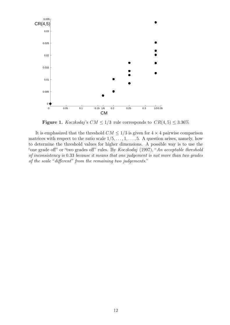
Based on Theorem 4.1 and Table 3, the inconsistency ratio CR(4, 5) can be deter-mined. By generating all the possible PRM (96 = 531441 matrices) with CM ≤ 1/3(1377 matrices) on the ratio scale 1/5, . . . , 1, . . . , 5, Figure 1 shows that the possiblevalues of CM under 1/3 are from the set {0, 1/6, 1/5, 1/4, 1/3} and the total number ofdifferent pairs (CM, CR(4, 5)) is 14. We can state that the threshold CM ≤ 1/3 corre-sponds to CR(4, 5) ≤ 0.0336 (3.36%). It follows that Koczkodaj ’s inconsistency index for4× 4 pairwise comparison matrices with respect to ratio scale 1/5, . . . , 1, . . . , 5, is stricterthan that of Saaty ’s. It is noted that the 10% rule allows much higher CM -inconsistencywhen using the ratio scale 1/9, . . . , 1, . . . , 9. An example is as follows:

A =

1 1/8 2 6

8 1 7 9

1/2 1/7 1 2

1/6 1/9 1/2 1

,

where CR = CR(4, 9) = 9.47% and CM = 0.8125.

11

0 0.05 0.1 0.15 1/6 0.2 0.25 0.3 1/3 0.35

0

0.005

0.01

0.015

0.02

0.025

0.03

0.035

CR(4,5)

CM

Figure 1. Koczkodaj ’s CM ≤ 1/3 rule corresponds to CR(4, 5) ≤ 3.36%

It is emphasized that the threshold CM ≤ 1/3 is given for 4× 4 pairwise comparisonmatrices with respect to the ratio scale 1/5, . . . , 1, . . . , 5. A question arises, namely, howto determine the threshold values for higher dimensions. A possible way is to use the“one grade off” or “two grades off” rules. By Koczkodaj (1997), “An acceptable thresholdof inconsistency is 0.33 because it means that one judgement is not more than two gradesof the scale “different” from the remaining two judgements.”

12

The

largestelem

ent

(M)

RI(n

,M

)3

45

67

89

1011

1213

1415

30.11

80.18

50.25

20.32

10.38

90.45

70.52

50.59

20.65

80.72

50.79

10.85

70.92

2

40.18

50.29

50.40

90.52

60.64

40.76

40.88

41.00

51.12

61.24

71.36

91.49

11.61

1

50.22

50.36

10.50

40.65

10.80

20.95

51.10

91.26

41.42

11.57

81.73

51.89

42.05

2

Matrix

60.25

10.40

40.56

50.73

10.90

11.07

41.24

91.42

61.60

31.78

31.96

22.14

22.32

4

size

70.26

90.43

30.60

60.78

40.96

71.15

31.34

11.53

11.72

21.91

42.10

82.30

22.49

6

(n)

80.28

20.45

40.63

50.82

21.01

31.20

71.40

41.60

31.80

32.00

42.20

62.40

92.61

3

90.29

20.47

00.65

70.85

01.04

71.24

81.45

11.65

61.86

22.06

92.27

82.48

72.69

7

100.30

00.48

20.67

30.87

11.07

31.27

81.48

61.69

51.90

62.11

82.33

12.54

52.75

9

Tab

le3.

Averag

evalueof

theinconsistencyindicesof

rand

omP

RM

depe

ndingon

thelargestelem

entof

theratioscale

Let us consider the general form of 3× 3 positive reciprocal matrices formulated in(3.1). In the consistent cases, a = b/c, 1/a = c/b, b = ac, 1/b = 1/(ac), c = b/a,1/c = a/b. In the inconsistent cases, the approximation of an element by the other twoelements can be considered by the grade difference

GD(a, b, c) = min{

max {| a− b/c | , | 1/a− c/b |},

max {| b− ac | , | 1/b− 1/(ac) |} , max {| c− b/a | , | 1/c− a/b |}}

.

Thus, the one grade off rule and the two grades off rule are

GD(a, b, c) ≤ 1 and GD(a, b, c) ≤ 2,

respectively.

In the case of matrices A of higher orders, the one grade off rule and the two gradesoff rule (Koczkodaj et al., 1997) are

GD(A) = max{

GD(a, b, c) for each triad (a, b, c) in A}≤ 1 or 2.

Figure 2 shows that the threshold CM ≤ 1/3 corresponds to GD ≤ 2/3, which isclose to the one grade off rule.

0 0.05 0.1 0.15 0.2 0.25 0.3 0.350

0.1

0.2

0.3

0.4

0.5

0.6

0.7

CM

GD

Figure 2. CM ≤ 1/3 threshold corresponds to GD ≤ 2/3

14

5. Inconsistency of random pairwise comparison matrices

Golden and Wang (1990) computed the random inconsistency indices and Forman(1990) the same for incomplete PRM. Dodd, Donegan and McMaster (1993) investigatedthe frequency distributions of random inconsistency indices and their statistical signif-icance levels. Lane and Verdini (1989) determined the exact distribution of randominconsistency indices for 3 × 3 matrices, and random samples of 2500 matrices wereproduced and analysed for 4 × 4 to 10 × 10 and selected higher-order matrices, as wellas stricter consistency requirements for 3 × 3 and 4 × 4 pairwise comparison matriceswere suggested. Standard 2000 generated randomly 1000 PRM, but restricted the CRn

as follows. For n = 3, 4 or 5, CRn < 0.1 was required, for n = 6, CRn < 0.2, and forn = 7, CRn < 0.3. The computer was very slow in generating the random, low CRn,PRM regarding sizes 6 and 7 and the results became more scattered as n increased. Ad-ditionally, regarding n = 7, there were no results for CRn < 0.1. Due to these conditions,the low CRn analysis was not run regarding matrices of sizes 8 and 9. A conclusion isthat Saaty ’s rule is statistically very strict for large PRM.

We have performed a statistical analysis of CR and CM inconsistencies. The aimof our simulation was to analyze the empirical distributions of the maximal eigenvaluesλmax of randomly generated pairwise comparison matrices. The elements aij (i < j) wererandomly chosen from the scale

1

9,1

8,1

7, . . . ,

1

2, 1, 2, . . . , 8, 9,

and aji is defined as1

aij

. In the paper, the assumption of equal probabilities is used.

In order to have equal probabilities ( 117), we used Matlab’s rand function for simulat-

ing uniform distribution, the period of which is 21492. We have computed the averagevalue of λmax of randomly generated pairwise comparison matrices which is the basisof the mean random consistency index (RIn). The values of λmax corresponding to theCRn = 10%, the number of matrices which satisfies the CRn ≤ 10%, GD ≤ 1 andGD ≤ 2 conditions were also computed. (It follows from the definition of CRn that – ifthe comparisons are carried out randomly – the expected value of CRn is 1.) In Table 4,n varies from 3 to 10, the sample size is 107 for all n.

In the case of 3× 3 matrices, the sample size 107 is much larger than the numberof different matrices 173 = 4913. Thus, many (or all) of the matrices may have beencounted more than once. The ratios of the numbers of matrices holding CR ≤ 10%,GD ≤ 1 and GD ≤ 2 compared to the sample size have been also computed if eachmatrix counted exactly once, and found to have almost the same results as above.

Our simulations are visualized in histograms, too. Figures 3.a – 3.h show the empir-ical distributions of λmax on the lower horizontal axis and the corresponding consistencyratio CRn on the upper horizontal axis. As n increases, the shape of distribution ofλmax gets similar to a normal one in our sample. For n = 3, a notable part of the ran-domly generated matrices satisfies the CRn ≤ 10% rule. The number of matrices withCRn ≤ 10% drastically decreases as n increases (see Table 4 ). Regarding n = 8, 9, 10,we have not found a matrix in the sample of ten million with acceptable inconsistency.Based on the results, it seems that the meaning of 10% for n = 3 is very different fromn = 8, which is one of the weaknesses of the inconsistency ratio by Saaty. It is alsointeresting that consistency and randomness do not exclude each other: 1.7% of 3 × 3random matrices (and 0.0014% of 4× 4 random matrices) are consistent.

15

nSa

mple

size

Averag

evalue

ofλ

max

RI n

λm

ax

correspo

ndingto

CR

=10

%

Num

berof

matrices

CR≤

10%

Num

berof

matrices

GD≤

1

Num

berof

matrices

GD≤

2

310

74.04

840.52

423.10

482.

08×

106

1.42×

106with

GD≤

12.

0×

106with

GD≤

2

1.42×

106

allw

ith

CR≤

10%

2.68×

106

2.0×

106with

CR≤

10%

410

76.65

250.88

424.26

53.

15×

105

2.76×

104with

GD≤

11.

55×

105with

GD≤

2

2.76×

104

allw

ith

CR≤

10%

1.7×

105

1.55×

105with

CR≤

10%

510

79.43

471.10

875.44

352.

39×

104

61with

GD≤

123

71with

GD≤

2

61allw

ith

CR≤

10%

2404

2371

with

CR≤

10%

610

712

.244

1.24

886.62

4477

00with

GD≤

113

with

GD≤

20

13allw

ith

CR≤

10%

710

715

.045

1.34

087.80

459

0with

GD≤

10with

GD≤

20

0

810

717

.831

1.40

048.98

310

00

910

720

.604

1.45

0510

.16

00

0

1010

723

.374

1.48

611

.337

40

00

Tab

le4.

Averag

evalueof

λm

axof

rand

omly

generatedpa

irwisecompa

risonmatrices,

RI n,the

numbe

rof

matriceswith

CR≤

10%,

GD≤

1an

dG

D≤

2

6. Inconsistency of asymmetry

A conceptual weakness of some weighting method is related to the issue of asymmetry.The question: “To what extent does alternative i dominate j?” may be replaced by thequestion “To what extent is j dominated by i?” The answers to these questions arelogically reciprocal. If a technique is applied first to the pairwise comparison matrix A,

yielding a solution w, and then to the transpose AT , yielding a solution w′ , is

wi

wj

=w′j

w′i

for every pair (i, j)?

EM does not possess this asymmetry property, since the principal right and lefteigenvectors of A are not elementwise reciprocal in the cases of inconsistent pairwisecomparison matrices. Consequently, a conceptual limitation of EM is the lack of asym-metry with respect to A and AT , which means that, for n ≥ 4, there exist, generally,two competing solutions (Johnson et al., 1979). Now, it will be shown that the propertyof asymmetry is related to the inconsistency.

Definition 6.1 Let A be a pairwise comparison matrix, w and w′ the priority vectors

of A and AT , respectively. The invariance under transpose holds if

wi ≥ wj implies w′i ≤ w

′j, ∀(i, j), i, j = 1, . . . , n. (6.1)

It follows from the definitions that LSM, χ2M and LLSM defined in Table 1 alwaysfulfil the property of invariance under transpose. SVDM takes this asymmetry, in somesense, into account.

Lemma 6.1 SVDM fulfils the invariance under transpose if and only if

uivi + 1

ujvj + 1≥ vi

vj

impliesuivi + 1

ujvj + 1≤ ui

uj

, ∀(i, j) i, j = 1, . . . , n, (6.2)

where u and v are the left and right singular vectors belonging to the largest singularvalue of A, respectively.

Proof. By the formula in Table 1, the invariance under transpose holds if and onlyif

ui +1

vi

≥ uj +1

vj

implies vi +1

ui

≤ vj +1

uj

, ∀(i, j) i, j = 1, . . . , n,

which is equivalent to

uivi + 1

ujvj + 1≥ vi

vj

impliesuivi + 1

ujvj + 1≤ ui

uj

, ∀(i, j) i, j = 1, . . . , n.

¥

108 matrices of size 5× 5 have been generated randomly in order to detect the rankreversals of the weights computed from the left and right eigenvectors. Based on ourhypothesis, the frequency of rank reversals varies as the CR inconsistency ratio changes.By Table 5 and Figure 4, the frequency of rank reversals increases as the CR increases.We can conclude that the larger the CR-inconsistency is, the more often the EM violatesthe property of invariance under transpose. Since no “cut off” point appears in Figure 4 ,this seems to be another reason for reconsidering the asymmetry property.

17

The next example (Dodd et al., 1995) shows that a good inconsistency ratio CR doesnot exclude the rank reversal between the weights computed from the left and righteigenvectors. Let

A =

1 1 3 9 9

1 1 5 8 5

1/3 1/5 1 9 5

1/9 1/8 1/9 1 1

1/9 1/5 1/5 1 1

,

where CR(A) = 0.0820, the weights of the right eigenvector

wT = (36.5652, 38.9564, 16.7155, 3.4693, 4.2936),

and the weights of the left eigenvector

w′T = (40.6431, 36.4208, 15.0669, 3.4391, 4.4302).

It is interesting that GD(A) = 4.1111. There remain open questions, namely, how todetect and eliminate the inconsistency of asymmetry.

18

Levels ofinconsistencyratio CR

Number of rank reversalsof the weight vectors

corresponding to the leftand right eigenvectors

Number ofmatrices

Frequency ofrank reversals

CR ≤ 0.01 8 162 0.0490.01 < CR ≤ 0.02 81 1138 0.0710.02 < CR ≤ 0.03 288 3414 0.0840.03 < CR ≤ 0.04 685 7130 0.0960.04 < CR ≤ 0.05 1253 12645 0.0990.05 < CR ≤ 0.06 2096 19827 0.1060.06 < CR ≤ 0.07 3342 29686 0.1130.07 < CR ≤ 0.08 5284 41400 0.1280.08 < CR ≤ 0.09 7896 55105 0.1430.09 < CR ≤ 0.10 10819 70885 0.1530.10 < CR ≤ 0.11 14371 88104 0.1630.11 < CR ≤ 0.12 18743 1.07 × 105 0.1740.12 < CR ≤ 0.13 23362 1.28 × 105 0.1820.13 < CR ≤ 0.14 27841 1.50 × 105 0.1850.14 < CR ≤ 0.15 33402 1.73 × 105 0.1930.15 < CR ≤ 0.16 39344 1.97 × 105 0.1990.16 < CR ≤ 0.17 44851 2.21 × 105 0.2030.17 < CR ≤ 0.18 50847 2.46 × 105 0.2070.18 < CR ≤ 0.19 57625 2.69 × 105 0.214

0.19 < CR not analysed 9.82 × 107 not analysed

Table 5. Frequency of rank reversals of the weight vectors corresponding to the leftand right eigenvectors with respect to different levels of inconsistency ratio CR

Figure 4. Frequency of rank reversals of the weight vectors corresponding to the leftand right eigenvectors with respect to different levels of inconsistency ratio CR

19

7. Concluding remarks

In the paper, some theoretical and numerical properties of Saaty ’s and Koczkodaj ’sinconsistencies of PRM are investigated. Based on the results, it seems that the deter-mination of the inconsistency of PRM has some drawbacks, thus the improvement of thenotion of inconsistency should be necessary.

Related to Saaty ’s inconsistency ratio, some basic questions are as follows:What is the relation between an empirical matrix from human judgements and a ran-

domly generated one? Is an index obtained from several hundreds of randomly generatedmatrices the right reference point for determining the level of inconsistency of pairwisecomparison matrix built up from human decisions, for a real decision problem? How totake the size of matrices into account in a more precise form?

Related to Koczkodaj ’s consistency index, a major question seems to be the elabora-tion of the thresholds in higher dimensions or to replace the index by a refined grade offrule.

The existence of the inconsistency of asymmetry shows the complexity of the problem.By the example in Section 6, Saaty ’s consistency of PRM is insufficient to exclude asym-metric inconsistency, therefore, this latter should be considered as a separate issue. Thus,it seems that only one inconsistency index is insufficient for describing the inconsistency.

Acknowledgement

The authors thank the Referees for the remarks and advice. The distinction of Saaty ’sand Koczkodaj ’s inconsistencies, given by one of the Referees, is emphasized.

20

References

Aguarón, J. and Moreno-Jiménez, J.M., The geometric consistency index: Approxi-mated thresholds, European Journal of Operational Research 147 (2003) 137-145.

Borda, J.C. de, Mémoire sur les électiones au scrutin, Histoire de l’Académie Royaledes Sciences, Paris, 1781.

Chu, A.T.W., Kalaba, R.E. and Spingarn, K., A comparison of two methods fordetermining the weight belonging to fuzzy sets, Journal of Optimization Theory andApplications 4 (1979) 531-538.

Condorcet, M., Essai sur l’application de l’analyse à la probabilité des décisions renduesá la pluralité des voix, Paris, 1785.

Crawford, G. and Williams, C., A note on the analysis of subjective judgment matrices,Journal of Mathematical Psychology 29 (1985) 387-405.

Dodd, F.J., Donegan, H.A. and McMaster, T.B.M., A statistical approach to consis-tency in AHP, Mathematical and Computer Modelling 18 (1993) 19-22.

Dodd, F.J., Donegan, H.A. and McMaster, T.B.M., Inverse inconsistency in analytichierarchy process, European Journal of Operational Research 80 (1995) 86-93.

Duszak, Z. and Koczkodaj, W.W., Generalization of a new definition of consistency forpairwise comparisons, Information Processing Letters 52 (1994) 273-276.

Forman, E.H., Random indices for incomplete pairwise comparison matrices, EuropeanJournal of Operational Research 48 (1990) 153-155.

Gass, S.I. and Rapcsák, T., Singular value decomposition in AHP, European Journal ofOperational Research 154 (3) (2004) 573-584.

Gass, S.I. and Standard, S.M., Characteristics of positive reciprocal matrices inthe analytic hierarchy process, Journal of Operational Research Society 53 (2002)1385-1389.

Golden, B.L. and Wang, Q., An alternative measure of consistency, in: AnalyticHierarchy Process: Applications and Studies, B.L. Golden, E.A. Wasil and P.T. Hacker(eds.), Springer-Verlag (1990) 68-81.

Jensen, R.E., Comparison of eigenvector, least squares, Chi square and logarithmic leastsquares methods of scaling a reciprocal matrix, Trinity University, Working Paper 127(1983). (http://www.trinity.edu/rjensen/127wp/127wp.htm)

Johnson, C.R., Beine, W.B. and Wang, T.J., Right-left asymmetry in an eigenvectorranking procedure, Journal of Mathematical Psychology 19 (1979) 61-64.

Koczkodaj, W.W., A new definition of consistency of pairwise comparisons,Mathematical and Computer Modelling 8 (1993) 79-84.

Koczkodaj, W.W., Herman, M.W. and Orlowski, M., Using consistency-driven pairwisecomparisons in knowledge-based systems, in: Proceedings of the sixth internationalconference on Information and knowledge management, ACM Press (1997) 91-96.

21

Lane, E.F. and Verdini, W.A., A consistency test for AHP decision makers, DecisionSciences 20 (1989) 575-590.

Monsuur, H., An intrinsic consistency threshold for reciprocal matrices, EuropeanJournal of Operational Research 96 (1996) 387-391.

Murphy, C.K., Limits on the analytic hierarchy process from its consistency index,European Journal of Operational Research 65 (1993) 138-139.

Peláez, J.I. and Lamata, M.T., A new measure of consistency for positive reciprocalmatrices, Computers and Mathematics with Applications 46 (2003) 1839-1845.

Saaty, T.L., The analytic hierarchy process, McGraw-Hill, New York, 1980 and 1990.

Saaty, T.L., Fundamentals of Decision Making, RSW Publications, 1994.

Standard, S.M., Analysis of positive reciprocal matrices, Master’s Thesis, GraduateSchool of the University of Maryland, 2000.

Stein, W.E. and Mizzi, P.J., The harmonic consistency index for the analytic hierarchyprocess, European Journal of Operational Research 177 (2007) 488-497.

Thorndike, E.L., A constant error in psychological ratings, Journal of AppliedPsychology 4 (1920) 25-29.

Thurstone, L.L., The method of paired comparisons for social values, Journal ofAbnormal and Social Psychology 21 (1927) 384-400.

Tummala, V.M.R. and Ling, H., A note on the computation of the mean randomconsistency index of the analytic hierarchy process (AHP), Theory and Decision 44(1998) 221-230.

Vargas, L.G., Reciprocal matrices with random coefficients, Mathematical Modelling 3(1982) 69-81.

22

List of Figures 3

3 4 5 6 7 8 9 10

0

500000

1000000

1500000

2000000

λmax

Number of matrices

0 1 2 3 4 5 6 C R

3.1048 4.0484λ

max(10%) λ

max(average)

0.1

10%

4 5 6 7 8 9 10 11 12 13 14

0

50000

100000

150000

200000

250000

300000

λmax

Number of matrices

0 1 2 3 C R

4.2652 6.6525λ

max(10%) λ

max(average)

0.110%

Figure 3.a λmax and CR valuesof 3× 3 random matrices

Figure 3.b λmax and CR valuesof 4× 4 random matrices

5 7 9 11 13 15 17 19

0

50000

100000

150000

200000

λmax

Number ofmatrices

0 1 2 3 C R

5.4435 9.4347λ

max(10%) λ

max(average)

0.110%

6 8 10 12 14 16 18 20

0

50000

100000

150000

200000

250000

300000

λmax

Number of matrices

0 1 2 C R

6.6244 12.2442λ

max(10%) λ

max(average)

0.1

10%

Figure 3.c λmax and CR valuesof 5× 5 random matrices

Figure 3.d λmax and CR valuesof 6× 6 random matrices

23

7 10 13 16 19 22

0

100000

200000

300000

400000

λmax

Number of matrices

0 1 2 C R

7.8045 15.0452λ

max(10%) λ

max(average)

0.110%

8 11 14 17 20 23 26

0

100000

200000

300000

400000

λmax

Number of matrices

0 0.5 1 1.5 C R

8.9831 17.8309λ

max(10%) λ

max(average)

0.1

10%

Figure 3.e λmax and CR valuesof 7× 7 random matrices

Figure 3.f λmax and CR valuesof 8× 8 random matrices

9 13 17 21 25 29 33

0

100000

200000

300000

400000

500000

λmax

Number ofmatrices

0 0.5 1 1.5 C R

10.1604 20.6044λ

max(10%) λ

max(average)

0.1

10%

10 15 20 25 30

0

100000

200000

300000

400000

λmax

Number ofmatrices

0 0.5 1 1.5 C R

11.3374 23.3743λ

max(10%) λ

max(average)

0.1

10%

Figure 3.g λmax and CR valuesof 9× 9 random matrices

Figure 3.h λmax and CR valuesof 10× 10 random matrices

24