On-road Heavy-duty Vehicle Emissions Monitoring System
17
On-road Heavy-duty Vehicle Emissions Monitoring System Gary A. Bishop,* Rachel Hottor-Raguindin, and Donald H. Stedman Department of Chemistry and Biochemistry, University of Denver, Denver Colorado 80208, United States Peter McClintock Applied Analysis, 13700 Marina Pointe Dr. Unit 301, Marina Del Rey, California 90292, United States Ed Theobald Envirotest Canada, 207-6741 Cariboo Rd., Burnaby British Columbia, Canada V3N4A3 Jeremy D. Johnson, Doh-Won Lee, † and Josias Zietsman Texas A&M Transportation Institute, 3135 TAMU, Texas A&M University, College Station, Texas 77843, United States Chandan Misra California Air Resources Board, 1001 I St. Sacramento, California 95814, United States * S Supporting Information ABSTRACT: The introduction of particulate and oxides of nitrogen (NO x ) after-treatment controls on heavy-duty vehicles has spurred the need for fleet emissions data to monitor their reliability and effectiveness. The University of Denver has developed a new method for rapidly measuring heavy-duty vehicles for gaseous and particulate fuel specific emissions. The method was recently used to collect 3088 measurements at a Port of Los Angeles location and a weigh station on I-5 in northern California. The weigh station NO x emissions for 2014 models are 73% lower than 2010 models (3.8 vs 13.9 gNO x /kg of fuel) and look to continue to decrease with newer models. The Port site has a heavy-duty fleet that has been entirely equipped with diesel particulate filters since 2010. Total particulate mass and black carbon measurements showed that only 3% of the Port vehicles measured exceed expected emission limits with mean gPM/kg of fuel emissions of 0.031 ± 0.007 and mean gBC/kg of fuel emissions of 0.020 ± 0.003. Mean particulate emissions were higher for the older weigh station fleet but 2011 and newer trucks gPM/kg of fuel emissions were nevertheless more than a factor of 30 lower than the means for pre-DPF (2007 and older) model years. ■ INTRODUCTION Diesel engines in the United States (U.S.) are major sources of fine particulate matter (PM) and oxides of nitrogen (NO x ) even though they generally represent <5% of the on-road vehicle fleet. 1-4 Many of the constituents found in diesel exhaust have also drawn the concerns of health officials for the past several decades. 5-7 For these reasons, reducing diesel exhaust emissions has been a major emphasis of state and federal regulators with the most recent U.S. and California limits for heavy-duty vehicles requiring a PM limit of 0.01 g/ bhp-hr (beginning with 2007 engines) and a NO x limit of 0.2 g/bhp-hr (beginning with some 2010 engines, Family Emission Limit rules allowing for emissions averaging and the banking and trading of emission credits permitted many 2010 and newer engines to exceed a rigid 0.2 g/bhp-hr limit until the credits were exhausted). 8-13 This has led to the introduction of new diesel engine after-treatment systems, most notably the diesel particulate filter (DPF) for PM reduction and selective catalytic reduction systems (SCR) for NO x control. The long- term in-service performance and durability of these devices is unknown and an important research question. U.S. and California diesel engine emission certification is accomplished with the use of an engine dynamometer and the Received: November 13, 2014 Revised: December 26, 2014 Accepted: January 5, 2015 Published: January 21, 2015 Article pubs.acs.org/est © 2015 American Chemical Society 1639 DOI: 10.1021/es505534e Environ. Sci. Technol. 2015, 49, 1639-1645
Transcript of On-road Heavy-duty Vehicle Emissions Monitoring System

On-road Heavy-duty Vehicle Emissions Monitoring System
Gary A. Bishop,* Rachel Hottor-Raguindin, and Donald H. Stedman
Department of Chemistry and Biochemistry, University of Denver, Denver Colorado 80208, United States
Peter McClintock
Applied Analysis, 13700 Marina Pointe Dr. Unit 301, Marina Del Rey, California 90292, United States
Ed Theobald
Envirotest Canada, 207-6741 Cariboo Rd., Burnaby British Columbia, Canada V3N4A3
Jeremy D. Johnson, Doh-Won Lee,† and Josias Zietsman
Texas A&M Transportation Institute, 3135 TAMU, Texas A&M University, College Station, Texas 77843, United States
Chandan Misra
California Air Resources Board, 1001 I St. Sacramento, California 95814, United States
*S Supporting Information
ABSTRACT: The introduction of particulate and oxides of nitrogen (NOx)after-treatment controls on heavy-duty vehicles has spurred the need for fleetemissions data to monitor their reliability and effectiveness. The University ofDenver has developed a new method for rapidly measuring heavy-duty vehiclesfor gaseous and particulate fuel specific emissions. The method was recentlyused to collect 3088 measurements at a Port of Los Angeles location and aweigh station on I-5 in northern California. The weigh station NOx emissionsfor 2014 models are 73% lower than 2010 models (3.8 vs 13.9 gNOx/kg offuel) and look to continue to decrease with newer models. The Port site has aheavy-duty fleet that has been entirely equipped with diesel particulate filterssince 2010. Total particulate mass and black carbon measurements showed thatonly 3% of the Port vehicles measured exceed expected emission limits withmean gPM/kg of fuel emissions of 0.031 ± 0.007 and mean gBC/kg of fuelemissions of 0.020 ± 0.003. Mean particulate emissions were higher for the older weigh station fleet but 2011 and newer trucksgPM/kg of fuel emissions were nevertheless more than a factor of 30 lower than the means for pre-DPF (2007 and older) modelyears.
■ INTRODUCTION
Diesel engines in the United States (U.S.) are major sources offine particulate matter (PM) and oxides of nitrogen (NOx)even though they generally represent <5% of the on-roadvehicle fleet.1−4 Many of the constituents found in dieselexhaust have also drawn the concerns of health officials for thepast several decades.5−7 For these reasons, reducing dieselexhaust emissions has been a major emphasis of state andfederal regulators with the most recent U.S. and Californialimits for heavy-duty vehicles requiring a PM limit of 0.01 g/bhp-hr (beginning with 2007 engines) and a NOx limit of 0.2g/bhp-hr (beginning with some 2010 engines, Family EmissionLimit rules allowing for emissions averaging and the bankingand trading of emission credits permitted many 2010 and
newer engines to exceed a rigid 0.2 g/bhp-hr limit until thecredits were exhausted).8−13 This has led to the introduction ofnew diesel engine after-treatment systems, most notably thediesel particulate filter (DPF) for PM reduction and selectivecatalytic reduction systems (SCR) for NOx control. The long-term in-service performance and durability of these devices isunknown and an important research question.U.S. and California diesel engine emission certification is
accomplished with the use of an engine dynamometer and the
Received: November 13, 2014Revised: December 26, 2014Accepted: January 5, 2015Published: January 21, 2015
Article
pubs.acs.org/est
© 2015 American Chemical Society 1639 DOI: 10.1021/es505534eEnviron. Sci. Technol. 2015, 49, 1639−1645

transient Federal Test Procedure cycle. Recent revisions haveincluded the possibility of on-road compliance monitoringusing portable emission monitors (PEMS).14,15 Thesetechniques, along with chassis dynamometer testing and on-road testing laboratories, provide highly detailed emissionmeasurements but are limited by cost, time, and effort in thenumber of heavy-duty vehicles (HDV) available for testingmaking it difficult to follow fleet-wide emission trends,especially when the means are dominated by a small percentageof malfunctioning vehicles.16−18
In-use fleet HDV emissions have been studied to date usingroad-way tunnels, mobile platforms, optical remote sensing andsampling individual truck plumes with a snorkel from bridgesand tunnels. Road-way tunnels allow for the unobtrusivemeasurement of fleet average emissions from large numbers ofvehicles at highway speeds but can be limited by location,driving mode and the inability to identify individualvehicles.19−21 The use of mobile measurement platforms is anovel approach for capturing vehicle plumes in all types ofdriving conditions but collecting a plume from a single vehicleand identifying its source can be a challenge.22 Optical remotesensing has been used in many locations to collect largenumbers of gaseous emission measurements on individualHDV’s identified by make and model year but is limited in itsability to collect detailed particle measurements.23−25 SniffingHDV exhaust stacks with a snorkel from an overpass or atunnel roof is one of the newer approaches that can captureboth gaseous and detailed particle data on individual HDV butto date has not linked any make and model year informationwith the measurements.26−28 All of these approaches canprovide large and robust data sets that when combined cancomplement one another in the study of fleet emission trends.Focusing on improving the measurements of individual HDV
gaseous and in particular particle emissions, the University ofDenver has developed a new technique which we have calledthe On-Road Heavy-Duty Vehicle Emissions MonitoringSystem (OHMS). To date we have tested the concept infour measurement campaigns. Two previous campaigns wereperformed in the summer of 2012 at the New Waverly weighstation on I-45 north of Houston, TX and the Nordel weighstation in Vancouver, BC.29,30 The two most recent campaignsdata will be discussed in this paper and were collected in 2013at a Port of Los Angeles location, previously used for ouroptical remote sensing measurements, and the Cottonwoodweigh station on I-5 near Redding CA.24,25
■ EXPERIMENTAL SECTION
OHMS is composed of three basic components, an exhaustcollection system, vehicle monitoring equipment and a suite ofgas and particle analysis instruments. The exhaust collectionsystem uses an extra-large event tent which can allow a heavy-duty truck to pass safely underneath. The tent acts as acontainment system to prevent the exhaust from simply risingand forces it to disperse in all directions, allowing the exhaustcollection pipe to capture a sample. The height of the tent hasbeen increased for each measurement campaign as overheighttrucks have proven to be more common than expected. Thethird version used in California, and the first to go unscathed byan overheight truck, is 15.2 m long, 4.6 m high and 5.5 m wide(see Figure 1). On the passenger side of the vehicle is a 3/4height tent wall, again to help contain the exhaust plume, whilethe driver side of the tent is open allowing an unobstructed
view for the driver. Each tent support standard is held to theground with concrete weights or two 200 L water barrels.Mounted to the tent roof underside on the passenger side of
the trucks, is the air intake pipe which is a 15.2 m long, 10.2 cmdiameter thin wall plastic pipe with holes drilled every 30.5 cmfor a total of 50 holes. The holes gradually decrease in size from∼2.5 cm at the entrance of the tent to ∼6.4 mm at the exit andare preferably angled toward the roadway. As the truck drivesthrough the tent its exhaust is integrated over the entire 15.2 m.Where the vehicles speed and acceleration matches the airspeed in the pipe, fresh exhaust from the truck arrives at eachsuccessive hole at the same time the exhaust sampled at theprior holes arrive, thus achieving a spatial and temporalintegration of the emissions of the tractor as it drives throughthe tent. An inline fan (Fantech FG 4XL, 135 cfm) brings thesampled exhaust down for the sampling lines (see SupportingInformation (SI) Figure S1). The entire pipe has a residence
Figure 1. Photographs of OHMS setups in Texas (top), VancouverBC (middle) and Cottonwood CA (bottom).
Environmental Science & Technology Article
DOI: 10.1021/es505534eEnviron. Sci. Technol. 2015, 49, 1639−1645
1640
time of approximately 8 s and rapidly dilutes the exhaust in theprocess by about a factor of 1000.Each truck either stops or slows to a crawl before entering
the tent where they are encouraged to accelerate as they drivethrough. The tent is long enough for many vehicles to usemultiple gears. Vehicle speeds and accelerations are measuredat the entrance and exit of the tent using two pairs of parallelinfrared beams (Banner Industries) 1.8m apart and approx-imately 1.2 m above the roadway. External exhaust pipetemperatures are estimated from thermal images collected oneach vehicle using a FLIR Thermovision A20 infrared (IR)camera. The thermographs are manually read and assigned amaximum temperature between 90 and 350 °C by comparisonto a lab created standard using a stainless steel exhaust pipe.The assigned temperatures assume a similar IR emissivity for allin-service exhaust pipes.25 Digital images are captured of eachvehicle’s license plate and of the driver’s side of each tractor.The license plates are matched against state records fornonpersonal vehicle information which generally includesmake, chassis model year, vehicle identification number(VIN), model and fuel type. The VIN (which we have notdecoded) will contain additional engine information but doesnot include engine certification standards or after-treatmentsystems installed. For the two California locations license plateinformation was obtained from the province of BritishColumbia, CA, and the states of California, Oklahoma, Oregonand Washington. The driver side images are used to identifytrucks with diesel exhaust fluid (DEF, 32.5% urea solution)tanks (not all tanks are on the driver’s side and many arehidden) denoting that the tractor is equipped with a NOx SCRsystem.The gaseous emission analyzers consist of a Horiba AIA-240
CO and CO2 nondispersive IR analyzer and two Horiba FCA-240 total hydrocarbon (THC)/nitrogen oxide (NO) or totalNOx analyzers. THC is only measured in one analyzer using aflame ionization detector while the NO/NOx detection methodutilizes ozone chemiluminescence. One FCA-240 is set up tomeasure only NO while the second incorporates a catalystenabling a total NOx (NO + nitrogen dioxide (NO2))measurement with the difference between the two analyzersequal to the amount of NO2 in the exhaust. The particlemeasurements use a Dekati digital mass monitor (DMM 230-A), which combines an aerodynamic and mobility particle sizedistribution measurement, to report total PM mass and particlenumber and a Droplet Measurement Technologies Photo-acoustic Extinctiometer (PAX, measures at 870 nm) fordetection of BC or soot (see SI Table S1 for analyzerspecifications).31 The Dekati DMM 230-A has been previouslyshown to correlate well with filter-based methods at the 2007Federal PM standard.32 All species are measured as a ratio toCO2 (see SI Figures S2−S5).
The CO2 analyzer’s maximum span adjustment is set at eachsite using a certified mixture of 3.5% CO2 in nitrogen (AirLiquide). All of the analyzers are adjusted to have a positiveoffset when sampling background air to preclude negativeconcentrations. Time alignment of the analyzers data streams ateach site are accomplished by filling a plastic syringe with all ofthe gaseous species and a small amount of black smoke andinjecting it about 0.5 m above the inline fan while recording allof the channels at 1 Hz. Peak positions relative to the CO2 peakare then stored by the data collection computer and used fortime alignment during the analysis. Daily calibrations of theanalyzers are made with multiple injections of a Bar-97 certifiedlow-range calibration gas (0.5% CO, 6% CO2, 200 ppmpropane, 300 ppm of NO in nitrogen) above the inline fan andaveraging the measured CO/CO2, HC/CO2, NO/CO2 andNOx/CO2 ratios and then dividing by the certified ratios. Theresults are then used to scale all of the measured vehicleemission ratios (see SI Table S2). The Dekati PM analyzer wascalibrated by the factory and does not require any additionalfield calibrations. The PAX BC instrument was calibrated in thelaboratory according to its standard operating procedures usingaerosolized ammonium sulfate particles for scatter and sootparticles from a propane flame for absorption.The gas analyzers are fed by a twin piston diaphragm pump
(KNF Neuberger, Inc. UN035.1.2ANP) delivering 55 l/min ofexhaust via 1/4 in. Teflon tubing via a water condensation trap.The two particle instruments each have internal samplingpumps and are fed by a separate 1/4 in. copper line (SI FigureS1 provides a schematic of the layout). An IR body sensorpositioned near the exit of the tent triggers the collection of 15or 20 s (depending on the site) of emissions data at 1 Hz fromall of the analyzers as the truck is exiting the tent. Theemissions time series for each instrument are time aligned andif sufficient amounts of CO2 are detected (minimum require-ments were for a 75 ppm rise above background) then eachspecies is correlated to CO2 and a linear least-squares line is fitto determine each slope (see SI Figures S2−S5). The slopes aredivided by the instrument ratio adjustment factor, previouslydetermined with the certified calibration gases, and convertedinto fuel-specific emissions of grams of pollutant per kilogramof fuel burned (g/kg) by carbon balance using the molecularweight of each species and 0.86 as diesel fuel’s carbon massfraction.We conducted 5 days of emission measurements using the
OHMS system at the Port of Los Angeles on lane no. 1 at theWater St. exit gate from the TRAPAC Inc. container operations(berths 135−139, April 22−26, 2013) in the South Coast AirBasin, that has been the site of four previous measurementcampaigns with our optical remote exhaust sensing system(FEAT), and at the California Highway Patrol Cottonwoodweigh station in northern CA (May 6−10, 2013) on
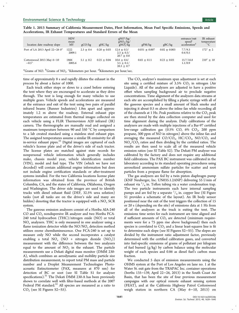
Table 1. 2013 Summary of California Measurement Dates, Fleet Information, Mean Fuel Specific Emissions, Speeds andAccelerations, IR Exhaust Temperatures and Standard Errors of the Mean
location date roadway slope
HDVmeanMY gCO/kg gHC/kg
gNOa/kg/gNO2/kg/gNOx
b/kg gPM/kg gBC/kg
entrance/exitspeedc
accelerationd
IR exhausttemperature
°C
Port of LA 2013 April 22−26 0° 12222009.1
2.3 ± 0.4 0.20 ± 0.03 12.4 ± 0.3/2.3 ± 0.3/20.7 ± 0.8
0.031 ± 0.007 0.02 ± 0.003 7.7/9.30.4/0.5
172° ± 2
Cottonwood 2013 May 6−10−0.5°
18662005.6
5.1 ± 0.2 0.25 ± 0.04 10.6 ± 0.4/3.5 ± 0.1/20.3 ± 0.7
0.65 ± 0.11 0.23 ± 0.03 15.7/16.81.1/0.9
210° ± 10
aGrams of NO. bGrams of NO2.cKilometers per hour. dKilometers per hour/sec.
Environmental Science & Technology Article
DOI: 10.1021/es505534eEnviron. Sci. Technol. 2015, 49, 1639−1645
1641

northbound I-5 (bottom photo Figure 1).24,25 The finalemission databases with vehicle registration information foreach site will be available for download from our Web site atwww.feat.biochem.du.edu.
■ RESULTS AND DISCUSSION
The OHMS measurement technique has evolved and beenimproved with each setup. The dimensions of the tent havechanged slightly with each successive campaign, especially theheight which was increased each time due to collisions withover height trucks (see Figure 1). The proof of concept tests inTexas experienced the most problems with high temperatureand humidity levels necessitating improvements in the watertrap design and proving intolerable for two PAX BC detectors(which has since been corrected by the manufacturer). Inaddition both of our previous studies suffered a likelyoverestimation of NO2 and total NOx emissions due to poorfield calibrations used to estimate the NOx analyzers NO2
conversion efficiencies which has also been corrected (see SI).Table 1 summarizes the data collected for the two California
locations with sampling dates, number of trucks successfullymeasured, their mean model year, fuel specific mean emissionswith standard errors of the mean calculated from the dailymeans, mean speeds and accelerations at the entrance and exitof the tent and the estimated mean IR exhaust temperatures ofthe trucks’ external exhaust pipes. NO2 emissions are calculatedby taking the difference between the total NOx analyzer and theNO analyzer. The accelerated retirement program previouslyinstituted by the Ports of Long Beach and Los Angelesmandated that all vehicles serving the port meet the Federal2007 PM emissions standard by 2010.33 Consequently, HDV’sat the Port are newer. The interstate truck fleet observed at theCottonwood weigh station is approximately 3.5 years olderthan the Port fleet and has higher mean CO and particulateemissions as a result, while the oxides of nitrogen meanemissions are similar. The higher than expected oxides ofnitrogen emissions for the newer Port fleet have been reportedbefore and are likely due to several factors including the slowerspeeds and higher load driving mode of accelerating their loadsfrom a complete stop.24,25 Port operations can lead to lowexhaust temperatures, poor SCR operation and higher NOx
emissions on the 2010 compliant HDV’s.34 In addition,although the Port fleet is newer, there are fewer 2010compliant HDV (only 11% of the Port fleet compared to18% of the weigh station fleet).We last measured HDV emissions at the Port of Los Angeles
with FEAT in the spring of 2012 when the fleet mean chassismodel year averaged 2009.3 which has changed little in theintervening year (2009.1 average for the 2013 measurements).The OHMS measurements have lower gCO/kg of fuel (2.3 ±
0.4 OHMS vs 8.2 ± 0.6 FEAT) and gHC/kg of fuel (0.20 ±
0.03 OHMS vs 3.7 ± 0.1 FEAT) means than the 2012 FEATmeasurements. Some of the differences are a direct result of thefleet differences between the two studies. In 2013 the OHMSsystem measured fewer natural gas powered trucks (3% OHMSvs 16% FEAT) than measured in 2012 by FEAT which havesignificantly higher CO and methane emissions. Figure 2compares the mean gNOx/kg of fuel emissions by model yearmeasured in 2013 with OHMS at the Port of Los Angeles andthe Cottonwood weigh station to our 2012 FEAT measure-ments at the same Port location and the Peralta weigh station inthe South Coast Air Basin in the Anaheim Hills.25 The errorbars plotted are standard errors of the mean determined from
the daily means. In general, chassis model years are a year olderthan the vehicles engine and it is the engines year ofmanufacture which defines Federal certification standards. Atthe Port the agreement between the two methods is quite goodwith the fleet mean emissions being statistically identical for theOHMS and FEAT data sets showing no emission deteriorationduring the intervening year.There are physical differences between the two weigh station
sites with Peralta having an uphill exit compared to Cotton-woods slightly downhill grade and the entrance ramp atCottonwood is significantly longer (1.1 km vs 0.3 km), whichmay account for the Cottonwood truck’s having slightly loweraverage IR exhaust temperatures (210 °C vs 225 °C). Speedsand accelerations are also slightly higher at Peralta. With thesecaveats the emission trends in Figure 2 are similar at the twoweigh stations with the highest NOx emissions during the late90s followed by a gradual reduction until the 2011 modelswhen a much faster reduction rate is observed as newer SCRequipped trucks are introduced. Because the Federal 2010HDV engine regulations allowed manufacturers the use ofemission credits to phase in 2010 compliant engines we stillhave not measured a fleet model year where all of the truckengines meet the 0.2 g/bhp-hr NOx standard. The 2014 modelyear trucks at Cottonwood (28 total) have mean NOx
emissions of 3.8 g/kg of fuel which is about 3 times higherthan an interpolated on-road standard of 1.33 g/kg of fuel byconverting the 0.2 g/bhp-hr standard into g/kg of fuelemissions assuming 0.15 kg of fuel are consumed per bhp-hr.35
The key advantage of the OHMS measurement system overFEAT is its ability to make particulate measurements. To datethere have only been a few studies in the literature that havereported particulate results for DPF equipped vehicles and acomparison of those results with the OHMS measurements isprovided in Table 2. Taking into account the load differences (a4% grade at highway speeds in the Caldecott Tunnel) and threeyears of fleet turnover to lower emitting HDV our 0.23 ± 0.03gBC/kg of fuel for the Cottonwood fleet is in generalagreement with on-road aethalometer measurements reportedby Dallmann et al. and statistically identical to the valuereported by Kozawa et al.22,26,27 For 2011 and newer trucks ourPort PM and BC measurements (133 measurements) arestatistically similar to the values May et al. reported for a 2010truck and only slightly higher than the data reported by Khalek
Figure 2. A comparison of the mean gNOx/kg of fuel emissions versuschassis model year between the OHMS results (filled symbols) andthe 2012 FEAT optical measurements (open symbols) at the Port ofLos Angeles site and the Cottonwood and Peralta weigh stationlocations. Error bars are standard errors of the means calculated fromthe daily means.
Environmental Science & Technology Article
DOI: 10.1021/es505534eEnviron. Sci. Technol. 2015, 49, 1639−1645
1642

et al. on 2010 engines.16,36 The PM and BC emissions for thisgroup are higher at Cottonwood. Both California locationssampled for the 2008−2010 model year group have higher BCemissions than the single DPF equipped 2007 truck May et al.measured, whereas the total PM measurements fall on eitherside. For non-DPF equipped trucks (generally pre-2008 chassismodel years and older) the on-road measurements fromCottonwood are higher for both PM and BC than the threevehicles May et al. tested in the laboratory.16 This is notsurprising since we have access to many more vehicles whichare unaware that they are going to be tested.Figures 3 and 4 are box and whisker plots by chassis model
year for the total PM (left gray shaded bars) and BC (right
white bars) measurements collected at the Port of Los Angelesand the Cottonwood weigh station. The box is defined as the25th, 50th, and 75th percentiles, the whiskers extend from the10th to the 90th percentiles and the data points are themeasurements beyond these percentiles. The filled square is themean value and split y-axes are used to cover the range of valueswhile preserving some of the detailed distribution of themajority of lower emitting vehicles. Within similar technologygroups we have aggregated some model years. The negativeratios reported provide a built in indicator for the noise level ofthe technique and a level above which an individualmeasurement’s significance can be judged. Negative ratios
occur when a zero emissions ratio (slope = 0) has noise thatresults in a fit with a negative slope. For a truly zero sample wewould expect half the readings to be negative and half positivewith a zero average. Negative results have not been removedand are included as measured in all of the calculations.In general, both PM and BC mean emissions increase with
age and BC emissions are lower than the total PMmeasurements. Beginning with the 2008 chassis model yearvehicles in Figure 4 it is clearly evident when the introductionsof DPFs occurred. Due to the limited number of model years inoperation at the Port the y-axis in Figure 3 can be expanded tosee the details of the interquartile range for each model yeargrouping. The size of the interquartile range, the extent of theoutliers and the skewness of the distribution (mean/medianratio increases) can be seen to increase with each successivemodel year group for both the PM and BC emissions. One istempted to speculate that this is the result of DPF deteriorationbut that determination will have to wait until we have additionaldata sets in order to distinguish “age” from model year. Againassuming that 0.15 kg of fuel is consumed per brake-horsepower we can convert the Federal 0.01 g/bhp-hr PMstandard to 0.07gPM/kg of fuel. If we follow light-duty OBDII“check engine light” logic and only consider trucks withemissions that are 3 times this standard (0.21gPM/kg) we findonly 3% of the 2007 and newer vehicles at the Port have PMmeasurements that exceed this level (40/1213) with 2010 andnewer trucks contributing only 6 of these exceedances (6/359).
Table 2. OHMS Particulate Emission Measurement Comparisons with Reported Literature Values
location (tests/samples) source chassis model year mean gPM/kg mean gBC/kg mean gEC/kg
laboratory (19) Khalek et al. 2011 0.0006 0.0001
Caldecott Tunnel (667) Dallmann et al. N.A. 0.54 ± 0.07a
Port of Oakland (418) Dallmann et al. N.A. 0.49 ± 0.08a
laboratory (13) May et al. 2010 0.007 ± 0.004b 0.0007 ± 0.002b
laboratory (12) May et al. 2007 0.15 ± 0.14b 0.0008 ± 0.0003b
laboratory (18) May et al. pre-2008 0.51 ± 0.05b 0.18 ± 0.03b
mobile platform (NA) Kozawa et al. N.A. 0.18 ± 0.1c
Port of LA (133) this work 2011 and newer 0.009 ± 0.004b 0.004 ± 0.006b
Port of LA (1070) this work 2008−2010 0.034 ± 0.007b 0.022 ± 0.003b
Cottonwood (335) this work 2011 and newer 0.03 ± 0.01b 0.013 ± 0.005b
Cottonwood (391) this work 2008−2010 0.3 ± 0.2b 0.059 ± 0.009b
Cottonwood (1094) this work pre-2008 0.96 ± 0.12b 0.36 ± 0.04b
a95% confidence intervals. bStandard errors of the mean. cOne standard deviation.
Figure 3. A box and whisker plot of gPM/kg (left and shaded) andgBC/kg of fuel (right) with a split y-axis versus chassis model year formeasurements collected at the Port of Los Angeles. The box is definedas the 25th, 50th, and 75th percentiles, the whiskers extend from the10th to the 90th percentiles, the circles lie beyond these percentilesand the filled square is the mean.
Figure 4. A box and whisker plot of gPM/kg (left and shaded) andgBC/kg of fuel (right) with a split y-axis versus chassis model year formeasurements collected at the Cottonwood weigh station. The box isdefined as the 25th, 50th and 75th percentiles, the whiskers extendfrom the 10th to the 90th percentiles, the circles lie beyond thesepercentiles and the filled square is the mean.
Environmental Science & Technology Article
DOI: 10.1021/es505534eEnviron. Sci. Technol. 2015, 49, 1639−1645
1643

At the Cottonwood weigh station there are more measure-ments above 0.21gPM/kg of fuel with 9% of the 2008 andnewer trucks (67/726), which also includes a higher percentageof 2010 and newer vehicles (31/432) than at the Port. Thelargest gPM/kg of fuel measurement was recorded from a 2009Kenworth, whose white smoke emissions were 73.8 g/kg offuel, accounting for the large increase in the 2009 mean PMemissions. The pre-DPF equipped trucks measured at Cotton-wood (generally 2007 and older), as expected have consistentlyhigher PM and BC emissions with a noticeable limit inemissions around 20 g/kg. There are two exceptions, a 2000Peterbilt with BC emissions of 25 g/kg of fuel and the 2009Kenworth previously mentioned. Since both particle instru-ments have cut-offs on the maximum size of particles that canbe sampled this will produce an upper limit on themeasurements that will be difficult to exceed without asignificant increase in the total number of small particles andthat may be the case for these two vehicles.Figure 5 plots the gBC/kg of fuel against gPM/kg of fuel for
the 107 vehicles at both locations, selected for PM emissions
greater than 0.21gPM/kg. If we exclude the 2009 Kenworthfrom the Cottonwood correlation, the increases in total particlemass correlate well (R2 of 0.75 with a slope of 0.4 atCottonwood and R2 of 0.93 with a slope of 0.6 at the Port) withthe increases in BC. The Cottonwood data’s (67 measurementsfrom 65 vehicles, filled circles) BC measurements are obviouslynoisier than similar measurements at the Port of Los Angeles(40 measurements from 36 vehicles, empty triangles).Contributing factors may include having to use generatorpower at Cottonwood and its audible noise affecting the PAXunit. Also the exhaust plumes at Cottonwood on average weresmaller (maximum CO2 of Δ350 ppm vs Δ400 ppm at thePort) and all of the larger negative gBC/kg of fuelmeasurements in Figure 5 are associated with small plumes.Confounding sources of emissions exist from transportation
refrigeration units (TRUs) and emissions from the contents ofthe trailers. We were able to identify 62 vehicles that had activeTRUs but saw no significant changes in NOx or particulateemissions. Since TRU engines cycle with temperature demandwe were not able to certify that the engine was actually in-use.We were also able to identify 90 vehicles with cattle transporttrailers in tow. These vehicles increase the mean gHC/kg offuel emission by ∼12% which is undoubtedly an increase inmethane emissions from the contents of the trailers.Going forward the OHMS measurement method is a new
tool that can be used to collect large numbers of gaseous and
particulate emission measurements from in-use heavy-dutyfleets in the U.S. The results discussed here are already asignificant contribution to realistic on-road HDV emissionsdata; we currently have plans to repeat the measurements at thetwo California locations in the spring of 2015 and 2017 whichwill hopefully allow us to study the important issue of in-usedeterioration of these vehicles NOx and PM after-treatmentsystems. It is also possible to envision using this method atpermanent locations that would allow year round sampling tocapture even larger segments of the HDV fleet.
■ ASSOCIATED CONTENT
*S Supporting Information
Supplementary figures (S1 to S7) and Tables (S1 to S2)referenced in the text. This material is available free of chargevia the Internet at http://pubs.acs.org.”
■ AUTHOR INFORMATION
Corresponding Author
*Phone (303) 871-2584; e-mail: [email protected].
Present Address†D-W.L.: California Air Resources Board, 9480 Telstar Ave.Suite 4, El Monte, CA 91731.
Author Contributions
The manuscript was written through contributions of allauthors. All authors have given approval to the final version ofthe manuscript.
Notes
The authors declare no competing financial interest.
■ ACKNOWLEDGMENTS
This paper is a result of work supported by the CaliforniaEnvironmental Protection Agency Air Resources Board (11-309), the North Central Texas Council of Governments,Envirotest Canada and the University of Denver. Results andconclusions presented here are solely the responsibility of theauthors and may not represent the views of the sponsors. Wegratefully acknowledge TraPac and the California HighwayPatrol for hosting our California measurements and IanStedman for support services.
■ REFERENCES
(1) Dallmann, T. R.; Harley, R. A. Evaluation of mobile sourceemission trends in the United States. J. Geophys. Res.: Atmos. 2010,115, D14305−D14312 DOI: 10.1029/2010JD013862.(2) McDonald, B. C.; Dallmann, T. R.; Martin, E. W.; Harley, R. A.Long-term trends in nitrogen oxide emissions from motor vehicles atnational, state, and air basin scales. J. Geophys. Res.: Atmos. 2012, 117(D18), 1−11 DOI: 10.1029/2012jd018304.(3) McDonald, B. C.; Gentner, D. R.; Goldstein, A. H.; Harley, R. A.Long-term trends in motor vehicle emissions in U.S. urban areas.Environ. Sci. Technol. 2013, 47 (17), 10022−10031 DOI: 10.1021/es401034z.(4) Pollack, I. B.; Ryerson, T. B.; Trainer, M.; Parrish, D. D.;Andrews, A. E.; Atlas, E. L.; Blake, D. R.; Brown, S. S.; Commane, R.;Daube, B. C.; de Gouw, J. A.; Dube,́ W. P.; Flynn, J.; Frost, G. J.;Gilman, J. B.; Grossberg, N.; Holloway, J. S.; Kofler, J.; Kort, E. A.;Kuster, W. C.; Lang, P. M.; Lefer, B.; Lueb, R. A.; Neuman, J. A.;Nowak, J. B.; Novelli, P. C.; Peischl, J.; Perring, A. E.; Roberts, J. M.;Santoni, G.; Schwarz, J. P.; Spackman, J. R.; Wagner, N. L.; Warneke,C.; Washenfelder, R. A.; Wofsy, S. C.; Xiang, B. Airborne and ground-based observations of a weekend effect in ozone, precursors, andoxidation products in the California South Coast Air Basin. J. Geophys.
Figure 5. Emissions of gBC/kg of fuel versus gPM/kg of fuel with asplit x-axis at the Cottonwood weigh station (filled circles) and thePort of Los Angeles (empty triangles) for HDV with a gPM/kg of fuelemissions greater than 0.21 gPM/kg of fuel.
Environmental Science & Technology Article
DOI: 10.1021/es505534eEnviron. Sci. Technol. 2015, 49, 1639−1645
1644

Res.: Atmos. 2012, 117 (D00V05), 1−14 DOI: 10.1029/2011JD016772.(5) Office of Environmental Health Hazard Assessment. Part B:Health Risk Assessment for Diesel Exhaust; California EnvironmentalProtection Agency: Sacramento, 1998; http://www.arb.ca.gov/regact/diesltac/partb.pdf.(6) California Air Resources Board. Risk Reduction Plan to ReduceParticulate Matter Emissions from Diesel-Fueled Engines and Vehicles;Sacramento, CA, 2000; http://www.arb.ca.gov/diesel/documents/rrpfinal.pdf.(7) Health Effects Institute. Traffic-related Air Pollution: A CriticalReview of the Literature on Emissions, Exposure, and Health Effects. ASpecial Report of the HEI Panel of the Health Effects of Traffic-related AirPollution; 2010; http://pubs.healtheffects.org/getfile.php?u=553.(8) NOx and particulate averaging, trading and banking for heavy-duty engines. In Code of Federal Regulations, Title 40, Section 86.007-15, 2001.(9) Emission standards and supplemental requirements for 2007 andlater model year diesel heavy-duty engines and vehicles. In Code ofFederal Regulations; Title 40 Section 86.007-−11, 2008.(10) U. S. Environmental Protection Agency; Air and Radiation,Highway diesel progress review; EPA420-R-02-016; 2002; www.epa.gov/oms/highway-diesel/compliance/420r02016.pdf.(11) Regulation to reduce emissions of diesel particulate matter,oxides of nitrogen and other criteria pollutants, from in-use heavy-dutydiesel-fueled vehicles. In California Code of Regulations; Title 13,Section 2025, 2008.(12) In-use on-road diesel-fueled heavy-duty drayage trucks. InCalifornia Code of Regulations, Title 13, Section 2027, 2008.(13) NOx plus NMHC and particulate averaging, trading and bankingfor heavy-duty engines. In Code of Federal Regulations; Title 40, Section86.004-15, 2000.(14) Amendments to the Regulation to Reduce Emissions of DieselParticulate Matter, Oxides of Nitrogen and Other Criteria PollutantsFrom In-Use On-Road Diesel-Fueled Vehicles. In California Code ofRegulations; Title 13, Section 2025, 2011.(15) Transient test cycle generation. In Code of Federal Regulations;Title 40, Section 86.1333, 2014.(16) May, A. A.; Nguyen, N. T.; Presto, A. A.; Gordon, T. D.; Lipsky,E. M.; Karve, M.; Gutierrez, A. r.; Robertson, W. H.; Zhang, M.;Brandow, C.; Chang, O.; Chen, S.; Cicero-Fernandez, P.; Dinkins, L.;Fuentes, M.; Huang, S.-M.; Ling, R.; Long, J.; Maddox, C.; Massetti, J.;McCauley, E.; Miguel, A.; Na, K.; Ong, R.; Pang, Y.; Rieger, P.; Sax, T.;Truong, T.; Vo, T.; Chattopadhyay, S.; Maldonado, H.; Maricq, M.M.; Robinson, A. L. Gas- and particle-phase primary emissions fromin-use, on-road gasoline and diesel vehicles. Atmos. Environ. 2014, 88,247−260 DOI: 10.1016/j.atmosenv.2014.01.046.(17) Johnson, K. C.; Durbin, T. D.; Jung, H.; Cocker, D. R.; Bishnu,D.; Giannelli, R. Quantifying in-use PM measurements for heavy dutydiesel vehicles. Environ. Sci. Technol. 2011, 45 (14), 6073−6079DOI: 10.1021/es104151v.(18) Wu, Y.; Carder, D.; Shade, B.; Atkinson, R.; Clark, N.; Gautam,M. In A CFR1065-Compliant Transportable/On-Road Low EmissionsMeasurement Laboratory with Dual Primary Full-Flow Dilution Tunnels;ASME 2009 Internal Combustion Engine Division Spring TechnicalConference, Milwaukee, WI, 2009; pp 399−410, 10.1115/ICES2009-76090.(19) Pierson, W. R.; Gertler, A. W.; Robinson, N. F.; Sagebiel, J. C.;Zielinska, B.; Bishop, G. A.; Stedman, D. H.; Zweidinger, R. B.; Ray,W. D. Real-world automotive emissionsSummary of studies in theFort McHenry and Tuscarora Mountain tunnels. Atmos. Environ. 1996,30 (12), 2233−2256.(20) Ban-Weiss, G. A.; McLaughlin, J. P.; Harley, R. A.; Lunden, M.M.; Kirchstetter, T. W.; Kean, A. J.; Strawa, A. W.; Stevenson, E. D.;Kendall, G. R. Long-term changes in emissions of nitrogen oxides andparticulate matter from on-road gasoline and diesel vehicles. Atmos.Environ. 2008, 42, 220−232 DOI: 10.1016/j.atmosenv.2007.09.049.(21) Fujita, E. M.; Campbell, D. E.; Zielinska, B.; Chow, J. C.;Lindhjem, C. E.; DenBleyker, A.; Bishop, G. A.; Schuchmann, B. G.;
Stedman, D. H.; Lawson, D. R. Comparison of the MOVES2010a,MOBILE6.2 and EMFAC2007 mobile source emissions models withon-road traffic tunnel and remote sensing measurements. J. Air WasteManage. Assoc. 2012, 62 (10), 1134−1149 DOI: 10.1080/10962247.2012.699016.(22) Kozawa, K. H.; Park, S. S.; Mara, S. L.; Herner, J. D. Verifyingemission reductions from heavy-duty diesel trucks operating onsouthern California freeways. Environ. Sci. Technol. 2014, 48 (3),1475−1483 DOI: 10.1021/es4044177.(23) Bishop, G. A.; Morris, J. A.; Stedman, D. H.; Cohen, L. H.;Countess, R. J.; Countess, S. J.; Maly, P.; Scherer, S. The effects ofaltitude on heavy-duty diesel truck on-road emissions. Environ. Sci.Technol. 2001, 35, 1574−1578 DOI: 10.1021/es001533a.(24) Bishop, G. A.; Schuchmann, B. G.; Stedman, D. H.; Lawson, D.R. Emission changes resulting from the San Pedro Bay, CaliforniaPorts truck retirement program. Environ. Sci. Technol. 2012, 46, 551−558 DOI: 10.1021/es202392g.(25) Bishop, G. A.; Schuchmann, B. G.; Stedman, D. H. Heavy-dutytruck emissions in the South Coast Air Basin of California. Environ. Sci.Technol. 2013, 47 (16), 9523−9529 DOI: 10.1021/es401487b.(26) Dallmann, T. R.; Harley, R. A.; Kirchstetter, T. W. Effects ofdiesel particle filter retrofits and accelerated fleet turnover on drayagetruck emissions at the Port of Oakland. Environ. Sci. Technol. 2011, 45,10773−10779 DOI: 10.1021/es202609q.(27) Dallmann, T. R.; DeMartini, S. J.; Kirchstetter, T. W.; Herndon,S. C.; Onasch, T. B.; Wood, E. C.; Harley, R. A. On-road measurementof gas and particle phase pollutant emission factors for individualheavy-duty diesel trucks. Environ. Sci. Technol. 2012, 46, 8511−8518DOI: 10.1021/es301936c.(28) Ban-Weiss, G. A.; Lunden, M. M.; Kirchstetter, T. W.; Harley,R. A. Measurement of black carbon and particle number emissionfactors from individual heavy-duty trucks. Environ. Sci. Technol. 2009,43, 1419−1424 DOI: 10.1021/es8021039.(29) Texas A&M Transportation Institute. Heavy-duty DieselInspection and Maintenance Pilot Program; College Station, TX, 2013;http://www.nctcog.org/trans/air/hevp/documents/NCTCOG_DieselIM_Final_Report_UpdatedOctober2013.pdf.(30) Envirotest Canada. Remote Sensing Device Trail for MonitoringHeavy-duty Vehicle Emissions; Burnaby, BC Canada, 2013; http://www.metrovancouver.org/about/publications/Publications/2013_RSD_HDV_Study.pdf.(31) Mamakos, A.; Ntziachristos, L.; Samaras, Z. Evaluation of theDekati Mass Monitor for the measurement of exhaust particle massemissions. Environ. Sci. Technol. 2006, 40 (15), 4739−4745DOI: 10.1021/es052302c.(32) Khalek, I. A. 2007 diesel particualte measurement researchPhase 1; Alpharetta, GA, 2005; http://www.crcao.com/reports/recentstudies2005/Final%20Rport-10415-Project%20E-66-Phase%201--R3.pdf.(33) San Pedro Bay Ports Clean Air Action Plan: About the CleanAir Action Plan. Port of Long Beach; Port of Los Angeles. http://www.cleanairactionplan.org/about_caap/default.asp (June 2011).(34) Misra, C.; Collins, J. F.; Herner, J. D.; Sax, T.; Krishnamurthy,M.; Sobieralski, W.; Burntizki, M.; Chernich, D. In-use NOx emissionsfrom model year 2010 and 2011 heavy-duty diesel engines equippedwith aftertreatment devices. Environ. Sci. Technol. 2013, 47 (14),7892−7898 DOI: 10.1021/es4006288.(35) Burgard, D. A.; Bishop, G. A.; Stedman, D. H.; Gessner, V. H.;Daeschlein, C. Remote sensing of in-use heavy-duty diesel trucks.Environ. Sci. Technol. 2006, 40, 6938−6942 DOI: 10.1021/es060989a.(36) Khalek, I. A.; Blanks, M. G.; Merritt, P. M. Phase 2 of theadvanced collarorative emissions study; Alpharetta, GA, 2013; http://crcao.org/reports/recentstudies2013/ACES%20Ph2/03-17124_CRC%20ACES%20Phase2-%20FINAL%20Report_Khalek-R6-SwRI.pdf.
Environmental Science & Technology Article
DOI: 10.1021/es505534eEnviron. Sci. Technol. 2015, 49, 1639−1645
1645

S-1
Supporting Information For:
On-road Heavy-duty Vehicle Emissions Monitoring System
Gary A. Bishop*, Rachel Hottor-Raguindin and Donald H. Stedman
Department of Chemistry and Biochemistry, University of Denver, Denver CO 80208
Peter McClintock
Applied Analysis, 13700 Marina Pointe Dr. Unit 301, Marina Del Rey, CA 90292
Ed Theobald
Envirotest Canada, 207-6741 Cariboo Rd., Burnaby British Columbia, Canada V3N4A3
Jeremy D. Johnson, Doh-Won Lee and Josias Zietsman
Texas A&M Transportation Institute, 3135 TAMU, Texas A&M University, College Station, TX
77843
Chandan Misra
California Air Resources Board, 1001 I St. Sacramento, CA 95814
*Corresponding author email: [email protected]; phone: (303) 871-2584
Summary of Supporting Information:
9 Pages (excluding cover):
Tables S1, S2
Figures S1 – S7

S-2
Table S1. Summary of instruments with corresponding operating principle, species measured,
range, repeatability and response time.
Model Operating Principle Species Range
(Repeatability)
Response
Time
Horiba AIA-240 Non-dispersive infrared
absorptiometry CO / CO2
CO – 0 to 1.0 vol%
(± 1% max value)
CO2 – 0 to 4.0 vol%
(± 1% max value)
1.5 s
Horiba FCA-240 Hydrogen flame
ionization detector THC
0 – 2000 ppm-C
(± 1% full scale)
1.5 s
Horiba FCA-240a Ozone
Chemiluminescence NO / NOx 0 to 500 ppm
NO 1.0 s
NOx 3.0 s
Dekati
DMM-230A
Density measurement
principle Particulate 0 to 1.2µm < 5 s
Droplet Measurement
Technologies PAXb
Photoacoustic
Extinctiometer (870nm)
Black
Carbon
< 1Mm-1
to
100,000Mm-1 < 10 s
a NOx measurements are collected using a second Horiba FCA-240 with a catalyst that converts
any NO2 to NO.
b Mass absorption cross section of 4.74 µm
-3 used to convert absorption to BC concentration.

S-3
Table S2. Field determined scaling factors for the OHMS gaseous analyzers.
Location CO/CO2 HC/CO2
NO/CO2 NOx/CO2
Port of LA 0.9 3.68 0.98 1.02
Cottonwood 0.8 2.94 1.04 1.02
Certified BAR-97 Low range cylinder with 0.5% CO, 6% CO2, 200ppm propane, 300ppm NO in nitrogen used to determine scaling factors.

S-4
Figure S1. Schematic drawing (not to scale) of the OHMS emission sampling setup.

S-5
Example Truck Plumes:
When a vehicle exits the tent an infrared body sensor triggers all of the cameras and the main
data collection cpu1 collects 1Hz voltage data from the five analyzers. The voltages are
converted to the appropriate units for each analyzer using each instrument’s response equations.
Figures S2 and S3 show the converted second by second data collected from a 2003 Freightliner
at the Cottonwood weigh station. These data have not been time aligned and the total NOx
analyzer and the two particulate instruments have noticeable time lags. Provided that the CO2
concentrations increase by more than 75ppm (our minimum plume size criteria) above the
background levels the data are time aligned and correlated against CO2 and a least squares line is
fit to the data and the slope of that line is the unadjusted fuel specific emissions ratio. Figures S4
and S5 show the correlation plots for the time aligned data for the five species measured and
each data set’s best fit line. Note that in Figure S4 the NOx/CO2 correlation data have been
vertically offset to better show the data points. For this vehicle the data points in the particulate
correlations have noticeably more scatter than the gaseous data which can result from higher
particle emissions during gear shifts at ratios to CO2 which are different than the dominant
driving mode.
Each linear least squares fit is quality checked against a set of error criteria and ratios meeting
those criteria are marked as valid in the data record. Valid ratios are adjusted by dividing by each
species scaling factors (see Table S2) determined using the gas calibration mixtures described in
the text. These adjusted ratios reported are mole ratios which are moles of the particular species
ratioed to the moles of carbon emitted as detailed in equation (1).
兼剣健結嫌 喧剣健健憲建欠券建兼剣健結嫌 系 噺 喧剣健健憲建欠券建系頚 髪 系頚態 髪 茎系 噺 岫喧剣健健憲建欠券建系頚態 岻岾 系頚系頚態峇 髪 な 髪 岾 茎系系頚態峇 岫な岻
Moles of pollutant are converted to grams by multiplying by the molecular weight of the species
and the moles of carbon in the exhaust are converted to kilograms by multiplying the result by
0.014 kg of fuel per mole of carbon in the fuel (this assumes a carbon mass fraction of 0.86),
assuming the fuel is stoichiometrically CH2.1

S-6
Figure S2. Concentration time series for the gaseous species from a 2003 Freightliner
measured at the Cottonwood weigh station. CO2 data (black circles) are plotted on the left
axis while the CO (black open diamonds), HC (red triangles), NO (blue filled diamonds)
and NOx (green pluses) are plotted on the right axis. Data are not time aligned.
Figure S3. Concentration time series for the particulate emissions from a 2003 Freightliner
measured at the Cottonwood weigh station. Total PM mass (grey circles) data are plotted
on the left axis and the BC mass (black diamonds) are plotted on the right axis. Data are
not time aligned.

S-7
Figure S4. Correlation plots for each of the gaseous species time aligned data
against CO2 for the 2003 Freightliner measured at the Cottonwood weigh station.
The NOx concentration data have been offset from their true values to clearly show
the data points and due to time offsets it only contains 14 data points.
Figure S5. Correlation plots for each of the particle species time aligned data
against CO2 for the 2003 Freightliner measured at the Cottonwood weigh station.
Due to time offsets the PM correlation only contains 13 data points and the BC
correlation only contains 14 data points. Also note that these correlations data
exhibit more scatter than the gaseous data likely a result of gear shifting that can
change the emission ratio very quickly.
S-8
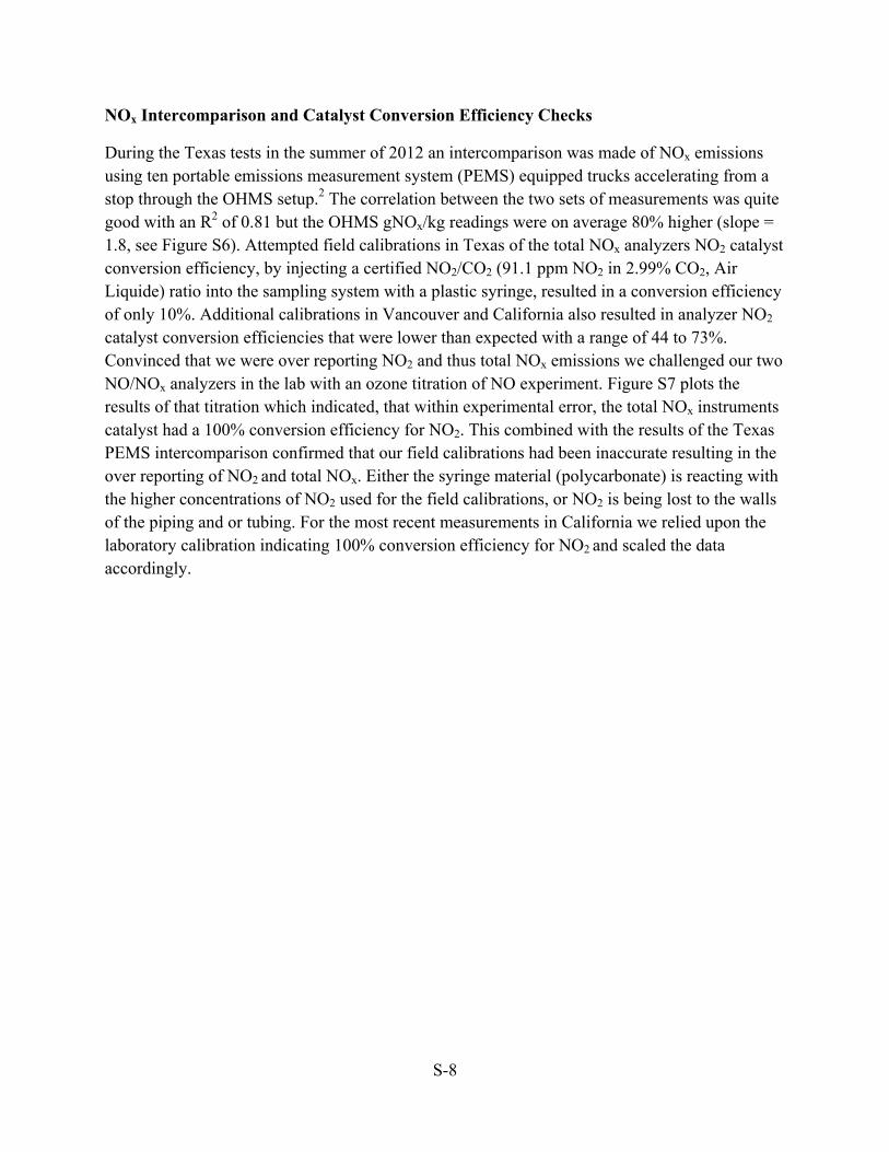
NOx Intercomparison and Catalyst Conversion Efficiency Checks
During the Texas tests in the summer of 2012 an intercomparison was made of NOx emissions
using ten portable emissions measurement system (PEMS) equipped trucks accelerating from a
stop through the OHMS setup.2 The correlation between the two sets of measurements was quite
good with an R2 of 0.81 but the OHMS gNOx/kg readings were on average 80% higher (slope =
1.8, see Figure S6). Attempted field calibrations in Texas of the total NOx analyzers NO2 catalyst
conversion efficiency, by injecting a certified NO2/CO2 (91.1 ppm NO2 in 2.99% CO2, Air
Liquide) ratio into the sampling system with a plastic syringe, resulted in a conversion efficiency
of only 10%. Additional calibrations in Vancouver and California also resulted in analyzer NO2
catalyst conversion efficiencies that were lower than expected with a range of 44 to 73%.
Convinced that we were over reporting NO2 and thus total NOx emissions we challenged our two
NO/NOx analyzers in the lab with an ozone titration of NO experiment. Figure S7 plots the
results of that titration which indicated, that within experimental error, the total NOx instruments
catalyst had a 100% conversion efficiency for NO2. This combined with the results of the Texas
PEMS intercomparison confirmed that our field calibrations had been inaccurate resulting in the
over reporting of NO2 and total NOx. Either the syringe material (polycarbonate) is reacting with
the higher concentrations of NO2 used for the field calibrations, or NO2 is being lost to the walls
of the piping and or tubing. For the most recent measurements in California we relied upon the
laboratory calibration indicating 100% conversion efficiency for NO2 and scaled the data
accordingly.

S-9
Figure S6. OHMS and portable emissions measurement system (PEMS) gNOx/kg of fuel
intercomparison conducted at the New Waverly weigh station on NB I-45 in Texas. PEMS
unit utilized was a SEMTECH-DS from Sensors, Inc. The least squares best fit line has a
slope of 1.8 and an R2 of 0.81.
Figure S7. NO (black dashed line) and NOx (red line) concentrations versus time during an ozone titration of NO. The large peak at the beginning is from opening the NO cylinder and after equilibration the ozone generator is turned on at a level which titrates about half of the NO in the sampling stream leaving the total NOx concentration unaffected.

S-10
1. FEAT Math II. Bishop, G. A.
http://www.feat.biochem.du.edu/assets/reports/FEAT_Math_II.pdf .
2. Texas A&M Transportation Institute, Heavy-duty Diesel Inspection and Maintenance Pilot
Program; College Station, TX, 2013;
http://www.nctcog.org/trans/air/hevp/documents/NCTCOG_DieselIM_Final_Report_UpdatedOc
tober2013.pdf.