
On Quantum Codes and Networks - Mathematics
211
On Quantum Codes and Networks Colin Michael Wilmott Technical Report RHUL–MA–2009–11 23 February 2009 Department of Mathematics Royal Holloway, University of London Egham, Surrey TW20 0EX, England http://www.rhul.ac.uk/mathematics/techreports
Transcript of On Quantum Codes and Networks - Mathematics

On Quantum Codes and Networks
Colin Michael Wilmott
Technical ReportRHUL–MA–2009–11
23 February 2009
Department of MathematicsRoyal Holloway, University of LondonEgham, Surrey TW20 0EX, England
http://www.rhul.ac.uk/mathematics/techreports

ON QUANTUM CODES ANDNETWORKS
Colin Michael Wilmott
Royal Holloway and Bedford New College,
University of London
Thesis submitted to
The University of London
for the degree of
Doctor of Philosophy
2008.

Declaration
The material contained herein is the result of my own studies. I declare that
foregoing is true and correct.
2
Acknowledgements
It is a real pleasure to acknowledge the help that I have received in bringing
this thesis to fruition. My supervisor Professor Peter Wild displayed patience,
understanding and insight during our many hours of discussion. To my family
and friends for their welcome distraction and source of excellent conversation.
To these, I offer my sincere thanks for their sustained support at all stages.
My graduate career was supported by an Engineering and Physical Sciences
Research Council Fellowship.
3
Abstract
The concern of quantum computation is the computation of quantum phe-
nomena as observed in Nature. A prerequisite for the attainment of such
computation is a set of unitary transformations that describe the operational
process within the quantum system. Since operational transformations in-
evitably interact with elements outside of the quantum system, we therefore
have quantum gate evolutions determined with less than absolute precision.
Consequently, the theory of quantum error-correction has developed to meet
this difficulty. Further, it is increasingly evident that much effort is being made
into finding efficient quantum circuits in the sense that for a library of realis-
able quantum gates there is no smaller circuit that achieves the same task with
the same library of gates. A reason for this concerted effort is primarily due
to the principle of decoherence. I give the construction for the set of unitary
transformations that describe an error model that acts on a d-dimensional
quantum system. I also give an overview of the theoretical framework asso-
ciated with such unitary transformations and generalise results to cater for
d-dimensional quantum states. I introduce two quantum gate constructions
that generalises the qubit SWAP gate to higher dimensions. The first of these
constructions is the WilNOT gate and the second is an efficient design also
based on binomial summations. Both of these constructions yield a quan-
tum qudit SWAP gate determined only in the CNOT gate. Furthermore, the
task of constructing generalised SWAP gates based on transpositions of qudit
states is argued in terms of the signature of a permutation. Based on this ar-
gument, we show that circuit architectures completely described by instances
4

of the CNOT gate can not implement a transposition of a pair of qudits over
dimensions d = 3 mod 4. Consequently, our quantum circuits are of interest
because it is not possible to implement a SWAP of qutrits by a sequence of
transpositions of qutrits if only CNOT gates are used. I also give bounds
on numbers of quantum codes predicated on d-dimensional quantum systems,
and generalise the encoding and decoding architectures for qudit codes.
5

Contents
Declaration 2
Acknowledgements 3
Abstract 4
Contents 6
List of Tables 9
List of Figures 10
1 Introduction 12
1.1 Introduction to Quantum Mechanics . . . . . . . . . . . . . . 15
1.2 Introduction to Coding Theory . . . . . . . . . . . . . . . . . 21
2 Quantum Error Correction 27
2.1 The Channel . . . . . . . . . . . . . . . . . . . . . . . . . . . 27
2.2 An Error Model . . . . . . . . . . . . . . . . . . . . . . . . . . 34
2.3 Definition and basic properties . . . . . . . . . . . . . . . . . . 37
2.4 A Quantum Qudit Code . . . . . . . . . . . . . . . . . . . . . 43
2.5 Qudit Error Correction . . . . . . . . . . . . . . . . . . . . . . 45
3 Unitary Error Bases 50
3.1 Higher Dimensional Unitary Error Bases . . . . . . . . . . . . 52
3.2 Shift and Multiply Bases . . . . . . . . . . . . . . . . . . . . . 55
3.3 Nice Error Bases . . . . . . . . . . . . . . . . . . . . . . . . . 56
6

4 The Stabilizer Formalism 65
4.1 Basic Definitions . . . . . . . . . . . . . . . . . . . . . . . . . 66
4.2 Stabilizer Codes . . . . . . . . . . . . . . . . . . . . . . . . . . 67
4.3 On Stabilizer Equivalence . . . . . . . . . . . . . . . . . . . . 70
4.4 Error Correcting Capabilities . . . . . . . . . . . . . . . . . . 74
4.5 Encoding the Stabilizer . . . . . . . . . . . . . . . . . . . . . . 76
4.6 Network for Encoding . . . . . . . . . . . . . . . . . . . . . . 80
5 Quantum Computation 84
5.1 Introduction . . . . . . . . . . . . . . . . . . . . . . . . . . . . 84
5.2 Multiple Quantum Gates . . . . . . . . . . . . . . . . . . . . . 89
5.3 Quantum Circuits . . . . . . . . . . . . . . . . . . . . . . . . . 90
5.4 On Permutations . . . . . . . . . . . . . . . . . . . . . . . . . 97
5.4.1 On the swap of a pair of Qutrits . . . . . . . . . . . . . 99
5.5 On the swap of a pair of qudits . . . . . . . . . . . . . . . . . 102
6 On the WilNOT Gate 105
6.1 The WilNOT Gate . . . . . . . . . . . . . . . . . . . . . . . . 106
6.2 WilNOT Example: The Qutrit Case . . . . . . . . . . . . . . 121
6.3 On the WilNOT Gate over Even
Dimensions Greater than Two . . . . . . . . . . . . . . . . . . 136
7 On Binomial Summations and an Efficient Generalised Quan-
tum SWAP Gate 143
7.1 The Construction . . . . . . . . . . . . . . . . . . . . . . . . . 143
7.1.1 The case d = pm . . . . . . . . . . . . . . . . . . . . . 148
7.1.2 Examples . . . . . . . . . . . . . . . . . . . . . . . . . 152
7.2 On the cycle length of 〈aj mod pm〉 . . . . . . . . . . . . . . . 155
7

7.3 Efficient Qutrit SWAP . . . . . . . . . . . . . . . . . . . . . . 159
8 Examples of Qudit Codes 172
8.1 The Qudit Shor Code . . . . . . . . . . . . . . . . . . . . . . 172
8.2 Qudit Stabilizer Codes . . . . . . . . . . . . . . . . . . . . . . 175
8.3 Constructing the Normaliser N (S) . . . . . . . . . . . . . . . 180
8.4 Encoding a Qudit Stabilizer Code . . . . . . . . . . . . . . . . 183
8.5 Correcting Procedure . . . . . . . . . . . . . . . . . . . . . . . 190
8.6 Complexity of a Qudit Stabilizer Code . . . . . . . . . . . . . 192
Appendix 195
Bibliography 199
8

List of Tables
7.1 Cycle length of∑j/d
i=0
(j−(d−1)i
i
)mod d. . . . . . . . . . . . . . . 157
8.1 The stabilizer for a five qutrit code. . . . . . . . . . . . . . . 176
8.2 The stabilizer for a nine qutrit code. . . . . . . . . . . . . . . 180
8.3 Algorithm to compute an encoding network for a qudit code. . 185
8.4 The stabilizer for a five qudit code derived from the five qubit
code. . . . . . . . . . . . . . . . . . . . . . . . . . . . . . . . 194
9

List of Figures
2.1 Generalised Bell State. . . . . . . . . . . . . . . . . . . . . . . 29
2.2 Quantum channel for teleporting a qudit. . . . . . . . . . . . . 31
2.3 Non-demolition measurement circuit. . . . . . . . . . . . . . . 47
4.1 Encoding network for X∗M . . . . . . . . . . . . . . . . . . . . 82
4.2 Encoding network for X∗MZ
∗M . . . . . . . . . . . . . . . . . . . 83
4.3 An Encoding Network for the [[8, 3, 5]] qubit code. . . . . . . . 83
5.1 Controlled-NOT produces entangled states. . . . . . . . . . . . 89
5.2 Quantum circuit swapping two qubits. . . . . . . . . . . . . . 91
5.3 Matrix representations of CNOT types. . . . . . . . . . . . . . 100
6.1 The WilNOT Gate; A Generalised SWAP Gate. . . . . . . . 107
6.2 WilNOT gate; Stage 2, steps j = 1, 2. . . . . . . . . . . . . . . 110
6.3 WilNOT gate; Stage 2. Algorithm step operates on successive
pairs. . . . . . . . . . . . . . . . . . . . . . . . . . . . . . . . . 110
6.4 WilNOT gate; Stage 2, steps j = 1,. . . , d-1. . . . . . . . . . . 111
6.5 WilNOT gate; Stage 3, step j = d. . . . . . . . . . . . . . . . 112
6.6 WilNOT gate; Stage 4, step j = d + 1. . . . . . . . . . . . . . 112
6.7 WilNOT gate; Stage 5, step j = d + 2. . . . . . . . . . . . . . 113
6.8 Qutrit WilNOT SWAP Network. . . . . . . . . . . . . . . . . 121
6.9 WilNOT gate over dimensions d = 0 mod 2; Stage 3. . . . . . 137
6.10 Pξ − 1 gates on pairs (ik, ik+1). . . . . . . . . . . . . . . . . . . 140
6.11 d− ξ gates on (id−2, id−1). . . . . . . . . . . . . . . . . . . . . 141
10

7.1 Binomial summation Quantum SWAP network construction over
dimension 4. . . . . . . . . . . . . . . . . . . . . . . . . . . . . 144
7.2 Quantum SWAP gate for qutrit states. . . . . . . . . . . . . . 159
8.1 Encoding and decoding circuit for the Shor qudit code. . . . . 173
8.2 Encoding circuit for a five qutrit code. . . . . . . . . . . . . . 189
8.3 Encoding circuit for a nine qutrit code. . . . . . . . . . . . . . 193
11

Chapter 1
Introduction
The desire to comprehend philosophies at the edge of possibility continues to
be a source of advancement today as it has been at any other time in his-
tory. If such a premise is taken to be a departure point in the challenge to
extend the boundaries of knowledge then theoretical and technical innovation
will abide. The Theory of Quantum Computation continues to advance our
understanding of information as established in the seminal work of Shannon
through an innovative analysis of the nature of noise. This development of a
quantum mechanical computing framework has redefined quantum computa-
tion and inspires discoveries whose very nature lie at the frontier of reality.
Modern computing begins with the pioneering work of Charles Babbage
and Alan Turing. An analytical machine put forward by Babbage conceived
the principle on which modern computing rests. Over a century later, Turing
improved upon the ideas of Babbage by devising a programmable means that
would become a basis for the description of computing logic. This model of
computation was then strengthened to illustrate the universal nature. This
became known as the Church-Turing thesis [89] and acknowledges the equiv-
alence between the principles of the Turing machine and the work of Alonzo
Church in lambda calculus. However, it is the nature of innovation to challenge
12

common perception, and challenges from different forms of efficient computa-
tion coupled with the emergence of randomised algorithmic protocols have
recast the Church-Turing thesis. These challenges may be seen to either
strengthen the position of modern computing or illustrate the limitations in
which modern computing is envisaged.
Quantum mechanics offers a new direction in the field of computation with
an interpretation of system more profound than the classical interpretation of
computation. Whereas the state of a classical computation can be described in
terms of a set of observable elements, the state of a quantum computation can
not be observed but rather is interpreted through a wave function associated
with the system. The promise of a quantum computer rests with the com-
plexity advantage it has over its classical counterpart. This was first mooted
by Richard Feynman [29] in which he suggests that the intractable nature of
using classical computers to describe quantum phenonmen might be overcome
were one to design a computer that used quantum mechanical effects. In 1985
David Deutsch [24] proposed a model of a quantum computer that gave cre-
dence to Feynman’s conjecture. The insights of Feynman and Deutsch into
the theory of quantum compuation mirror the contributions made by Babbage
and Turing to classical computation.
The task of constructing a quantum computer is predicated on firstly re-
alising the inherent processing advantage of quantum compuation over its
classical analogue and secondly, and more importantly, on controlling the sen-
sitive quantum interference effects that explain the source of its computational
power. However quantum computations also produce interactions between
sensitive quantum information and noise in the system and this interaction
results in decoherence, an outcome that destroys quantum information. Deco-
herence is an inevitable feature of quantum computation, and therefore, it is
13

of fundamental importance that any coupling between information and noise
be controlled to within a suitable degree of precision. A number of proposals
have emerged in recent years that put forth descriptions for a complete physi-
cal model for quantum computation. The first proposal is the Linear Ion Trap
[17] which stores quantum information in a well-defined way. This technique
prepares two distinct states in a trap of an electric field by targeting each
state with a series of laser pulses. A second proposal uses Nuclear Magnetic
Resonance [37], NMR, to measure the average nuclear spin state of atomic
nuclei. Cavity Quantum Electrodynamics [87], QED, is another consideration
whereby photons assume quantum state representations which together with
cavity QED techniques permit the preparation of a quantum state.
Chapter 2 introduces a quantum channel that permits the transmission of
a high dimensional quantum information state called a qudit in the general
dimension d. This is followed by a study on noise associated with such qudit
information states. I then discuss the theoretical nature of the corresponding
error model in chapter 3 together with construction techniques. Chapter 4
describes the stabilizer formalism, a network to encode stabilizer codes and
provides a result analogous to the number of distinct bases of a classical code.
Chapter 5 gives an overview of quantum computation and introduces the ques-
tion of constructing a generalised quantum SWAP gate. Chapter 6 introduces
the first of our quantum gate constructions, the WilNOT gate, that describes
the construction of a generalised quantum SWAP gate. This is followed by
a second gate construction that describes an efficient generalised quantum
SWAP gate. In this instance, efficiency is determined by the fewest use of the
controlled-NOT gate that is required to compute the task. Finally, I discuss
a number of qudit codes in chapter 7 along with a result on the complexity
associated with the encoding of a qudit code.
14

1.1 Introduction to Quantum Mechanics
The consideration of information theory is the efficient transmission of infor-
mation from sender to receiver. Classical information is recorded in a sequence
of states over some finite alphabet Σ where it is most often maintained that
Σ = {0, 1}. The classical unit of information is represented by a bit over the
finite field F2. Quantum information theory is constructed under an analogous
concept. The single state of a quantum system over CΣ is called a ket and
is represented by a qubit over C2 which is associated with the computational
basis states |0〉 and |1〉 whereby
|ψ〉 = α |0〉 + β |1〉 , (1.1.1)
with α, β ∈ C and |α|2 + |β|2 = 1. If both α and β are non-zero then the
state |ψ〉 is a superposition state with amplitudes α and β. The information
source of a classical system is described by a set of probabilites and similarly,
a quantum information source associates a set of probabilites, described by
probability amplitudes |αi|2, to basis states |ψi〉. Furthermore, while an n-
dimensional state in Fn2 is required to represent n bits of classical information,
a 2n dimensional state in C2nis needed to describe n qubits. Therefore, the
quantum system must remember 2n complex numbers for an n qubit state,
and it is this property of quantum system that is used in quantum information
theory.
Let {|ψi〉 , i ∈ Σ} be a basis for CΣ for which |ψ〉 =∑
i∈Σ αi |ψi〉. Then
CΣ explains span and independence, however we require the concepts of angle
and length between vectors to endow the vector space CΣ with geometry. A
linear functional on a vector space is a scalar-valued function γ defined for
15

every vector |ζ〉 and |η〉 and scalars α1 and α2 with the property that
γ(α1 |ζ〉+ α2 |η〉) = α1γ(|ζ〉) + α2γ(|η〉). (1.1.2)
To every vector space CΣ, we have a corresponding dual space(CΣ)⊥
consisting
of all linear functionals on CΣ. The single state of a quantum system over
CΣ⊥is called a bra. In particular, if {|ψi〉 , i ∈ Σ} is a basis in CΣ, then there
is a uniquely determined basis {|ψj〉† , j ∈ Σ} in(CΣ)⊥
such that the linear
functional ψj(|ψi〉) is identically |ψj〉†(|ψi〉) = δij. In the language of Dirac, the
action of the conjugate linear functional ψj(|ψi〉) on CΣ is written and defined
to be 〈ψj|ψi〉 = δij. To each |γ〉 =∑
j∈Σ βj |ψj〉 and |ψ〉 =∑
i∈Σ αi |ψi〉 the
value of γ(|ψ〉) is determined by
γ(|ψ〉) = 〈γ|ψ〉 =∑
i,j∈Σ
β∗jαi〈ψj|ψi〉 =
∑
i,j∈Σ
β∗jαiδij =
∑
i∈Σ
β∗i αi. (1.1.3)
where * denotes complex conjugation. Consequently, we are equipped to in-
duce a geometry on CΣ by defining inner product (|γ〉 , |ψ〉) on |γ〉 and |ψ〉 as
γ(|ψ〉). A function (|γ〉 , |ψ〉) from CΣ × CΣ to C is an inner product on the
vector space CΣ if the following conditions are satisfied
1. (|ψ〉 , |ψ〉) ≥ 0 with equality if and only if |ψ〉 = 0
2.(|γ〉 ,
∑i∈Σ αi |ψi〉
)=∑
i∈Σ αi(|γ〉 , |ψi〉)
3. (|γ〉 , |ψ〉) = (|ψ〉 , |γ〉)∗
Hence, an inner product space is a vector space with an inner product. We
say |ψ〉 and |γ〉 are orthogonal if the associated inner product vanishes. Fur-
thermore, to each inner product space we can associate a canonical form by
defining the norm of |ψ〉
‖ |ψ〉 ‖ =√〈ψ|ψ〉. (1.1.4)
16

A unit ket is a state with ‖ |ψ〉 ‖ = 1. The basis set {|ψi〉 , i ∈ Σ} is called
orthonormal if for all |ψi〉 and |ψj〉 it follows that 〈ψi|ψj〉 = δij. A vector
space CΣ that is an inner product space and complete with respect to the
norm is then called a Hilbert space over H = CΣ. Furthermore, there is only
one Hilbert space in distinct dimensions up to isomorphism.
A linear operator M on the Hilbert space CΣ is a mapping that assigns to
every state |ζ〉 in CΣ a state M |ζ〉 in CΣ, in such a way that
M (|ζ〉+ |η〉) = M |ζ〉+M |η〉 . (1.1.5)
The study of linear operators is known to elicit a matrix representation in-
duced by way of linear functionals. Given a basis {|ψi〉 , i ∈ Σ} in CΣ with
a corresponding dual set {〈ψj| , j ∈ Σ} in CΣ⊥, we have it that M |ζ〉 =
∑i∈Σ ψi(|ζ〉) |ψi〉 =
∑i∈Σ αi |ψi〉 = |ψ〉. Since every state is a linear combi-
nation in |ψi〉, then M |ζ〉 = M(∑
j∈Σ αj |ψj〉) =∑
i∈Σ αij |ψi〉 , for j ∈ Σ.
Therefore, the set of linear functionals define M within a matrix formalism
where such form is called an outer product representation. Suppose |ζ〉 and
|ψ〉 are states in the Hilbert space CΣ, we define |ψ〉 〈ζ| to be the outer product
operator on CΣ that maps |ζ〉 to |ψ〉 and whose action is defined by
M(|ζ〉) = (|ψ〉 〈ζ|) |ζ〉 ≡ |ψ〉 〈ζ|ζ〉 = 〈ζ|ζ〉 |ψ〉 . (1.1.6)
An important consequence of the outer product formalism is the completeness
relation for orthonormal vectors. For an orthonormal basis {|ψi〉 , i ∈ Σ} for
CΣ, and arbitrary state |ψ〉 for which 〈ψi|ψ〉 = αi, we have it that
(∑
i∈Σ
|ψi〉 〈ψi|)|ψ〉 =
∑
i∈Σ
|ψi〉 〈ψi|ψ〉 =∑
i∈Σ
αi |ψi〉 = |ψ〉 . (1.1.7)
The equation∑
i∈Σ |ψi〉 〈ψi| = I is known as the completeness relation.
17

A more general linear operator describes a number of important analogs
in matrix algebra. Given the Hilbert space CΣ, let {〈ζ| , i ∈ Σ} be a set of
states in the dual space(CΣ)⊥
, then for any linear operator M we have a
corresponding linear functional ζ(M |ψ〉) on C. There exists a unique linear
operator M † on(CΣ)⊥
, with the property
(|ζ〉 ,M |ψ〉) = (M † |ζ〉 , |ψ〉), (1.1.8)
for all |ζ〉 and |ψ〉 in CΣ. The linear operator M † is called the adjoint of M .
If M = M †, then M is a Hermitian operator. If M is Hermitian then MM † =
M †M . An operator M is said to be unitary if M †M = I. Unitary operators
are an important concept in the Hilbert space because they ensure that any
action by such an operator conditioned on a ket preserves the unit condition
in a Hilbert space. Furthermore, if both M and N are Hermitian operators
then (NM)† = M †N † = MN . If NM is Hermitian, that is, (NM)† = NM ,
then we requireM †N † = NM , whence,M and N commute. The commutation
property holds special resonance in quantum mechanics where the commutator
between operators M and N is defined as
[M,N ] = MN −NM. (1.1.9)
The operators M and N are then said to commute if [M,N ] vanishes.
Let {|ψi〉 , i ∈ Σ} be a basis for the Hilbert space CΣ and write A =∑
i,j∈Σ αij |ψi〉 〈ψj|. Let {|ζk〉 , k ∈ Γ} be a basis for the Hilbert space CΓ and
write B =∑
k,l∈Γ βkl |ζk〉 〈ζl|. The operators A and B define a spectral repre-
sentation of the respective Hilbert spaces. The tensor product is an operation
that creates a vector space of dimension |Σ||Γ| from vector spaces with asso-
ciated dimensions |Σ| and |Γ|. A basis for the tensor product system A ⊗ B
associated with the Hilbert space CΣΓ is given by |ψi〉⊗ |ζk〉 , i ∈ Σ and k ∈ Γ
18
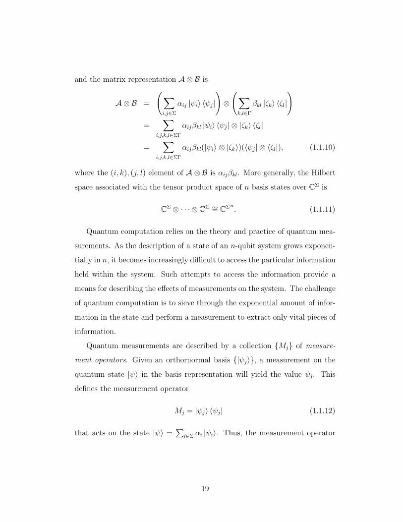
and the matrix representation A⊗ B is
A⊗ B =
(∑
i,j∈Σ
αij |ψi〉 〈ψj|
)⊗
(∑
k,l∈Γ
βkl |ζk〉 〈ζl|
)
=∑
i,j,k,l∈ΣΓ
αijβkl |ψi〉 〈ψj| ⊗ |ζk〉 〈ζl|
=∑
i,j,k,l∈ΣΓ
αijβkl(|ψi〉 ⊗ |ζk〉)(〈ψj| ⊗ 〈ζl|), (1.1.10)
where the (i, k), (j, l) element of A ⊗ B is αijβkl. More generally, the Hilbert
space associated with the tensor product space of n basis states over CΣ is
CΣ ⊗ · · · ⊗ CΣ ∼= CΣn. (1.1.11)
Quantum computation relies on the theory and practice of quantum mea-
surements. As the description of a state of an n-qubit system grows exponen-
tially in n, it becomes increasingly difficult to access the particular information
held within the system. Such attempts to access the information provide a
means for describing the effects of measurements on the system. The challenge
of quantum computation is to sieve through the exponential amount of infor-
mation in the state and perform a measurement to extract only vital pieces of
information.
Quantum measurements are described by a collection {Mj} of measure-
ment operators. Given an orthornormal basis {|ψj〉}, a measurement on the
quantum state |ψ〉 in the basis representation will yield the value ψj. This
defines the measurement operator
Mj = |ψj〉 〈ψj| (1.1.12)
that acts on the state |ψ〉 =∑
i∈Σ αi |ψi〉. Thus, the measurement operator
19

Mj extracts the component of a quantum state associated with |ψj〉,
Mj |ψ〉 = |ψj〉 〈ψj|ψ〉
=∑
i∈Σ
αiδij |ψj〉
= αj |ψj〉 . (1.1.13)
The probability, pj , that the result ψj occurs post measurement can be written
as
pj = 〈ψ|Mj |ψ〉
= 〈ψ|ψj〉〈ψj|ψ〉
=∑
i∈Σ
α∗iαiδij
= α∗jαj
= |αj|2 (1.1.14)
An important consequence of the measurement process is that it alters the
superposition state of a quantum state. If the result of the measurement of
|ψ〉 is ψj then we can describe the state post measurement as
|ψj〉 =1
αjMj |ψ〉
=Mj |ψ〉√〈ψ|Mj |ψ〉
. (1.1.15)
This result implies that additional information of the state |ψ〉 cannot be
collected post measurement since it is the nature of the measurement Mj
to distill a classical number ψj thereby collapsing |ψ〉 onto one of the basis
eigenstates |ψj〉. Furthermore, we note
〈ψ|M †jMj |ψ〉 = 〈ψj|α∗
jαj |ψj〉
= pj (1.1.16)
20

with
∑
j∈Σ
〈ψ|M †jMj |ψ〉 =
∑
j∈Σ
〈ψj|α∗jαj |ψj〉
=∑
j∈Σ
pj
= 1. (1.1.17)
Thus, the set of measurement operators {Mj} adhere to the completeness
equation which is expressed by the fact that the probabilities sum to unity.
Consequently, we have it that the measurement operator Mj admits the con-
dition
M †j = Mj = MjMj , (1.1.18)
illustrating that measurement operators associated with the basis states are
idempotent and Hermitian.
Hermitian operators play an important role in the theory of quantum com-
putation and communication and have a representation as meaningful entities,
or observables, of classical computation. This statement is qualified since Her-
mitian operators admit the result that measurement of a quantum state cor-
responds to classical outcome.
1.2 Introduction to Coding Theory
Coding theory is a branch of mathematics which seeks efficient solutions to the
many problems concerning the safe and accurate transfer of information from
one destination to another. Coding theory was initiated with a 1948 paper
by Claude E. Shannon [74] on the mathematics of communication and with a
1950 paper by Richard Hamming [39] on the correction of errors on magnetic
storage media which introduced the concept of error-correcting codes. As
21

our society becomes increasingly automated the applications of coding theory
become more diverse. From mobile telephone communications to interstellar
communications and compact disc recordings, coding theory has ensured its
prominance in modern society.
The coding channel is the physical medium through which we transmit
information. Within the spectrum of the channel there exist disturbances that
interact in an unwanted manner with the information as it passes through the
channel. More formally, these disturbances are referred to as noise, and result
in an information output that differs from the original information input.
Coding theory concerns itself with the problem of constructing efficient
error-correcting procedures to minimize the noise that act on the information
within the channel. A certain class of classical codes called BCH codes elicit
such an effective error-correcting procedure. The BCH codes, introduced in-
dependently by Bose and Ray-Chaudhuri [10] in 1960 and by Hocquenghem
[43] in 1959, rank among the most widely studied and practiced of all error-
correcting codes.
To speak of noise in terms of the errors it generates on the information
set is to speak on the choice of channel over which we send such information.
On the selection of an acceptable channel, we turn our considerations from
the communication device to devising procedures to encode and decode the
information for which the affects of noise are best minimized.
Information is transmitted over a channel. The channel takes the role
of a communication device in which there is a transmitter and a receiver.
Associated with the transmitter is an input alphabet Σ and corresponding to
the receiver we have an output alphabet Γ. We assume both Σ and Γ to be
of finite cardinality with Σ ⊆ Γ. The channel permits the transmission of
information by a sequence of characters from the finite alphabet Σ. A word is
22

a sequence of such alphabet characters. We denote Σn to be the set of words
of length n where Σn represents the Cartesian product of Σ with itself n times.
Furthermore, constraints are placed on Shannon’s general channel model.
The channel requires that the length of a word does not increase or decrease
during transmission. Secondly, associated with the input alphabet Σ and
output alphabet Γ, we have a graph with Σ on the left and Γ on the right
where the edge (σi, γi) is assigned with a probability of the channel changing
σi to γi. For each σi ∈ Σ, we have it that the sum of the probabilities on the
edged incident with it equals 1. In the theory of error-correcting codes, it is
often assumed that errors occur independently for each input character [52].
Shannon considered the difficulties in transmitting information over two
types of channel. Firstly, Shannon described a perfect, or noiseless, channel
whereby information is transmitted with perfect fidelity. However, the more
interesting concept of channel transmission considered by Shannon was that
of a noisy channel. The noisy channel is regarded as the cornerstone of Infor-
mation Theory by providing a beautiful description between two of the more
vital concerns of coding theory, namely, the maximal transmission of informa-
tion against a maximal correctness of transmission of such information. The
exact result allowed the understanding that should the flow of information
over the channel be less than the maximum permitted by the channel then
error-correction may take place. A commonly considered noisy channel is a
Binary Symmetric Channel (BSC). The alphabets Σ and Γ have cardinality
two and information is transmitted in a sequence of zeros and ones. The re-
liability of the binary symmetric channel is a real number p, (1/2 < p < 1),
where p represents the probability that the transmitted character is the same
as the received character.
A code C is a collection of words from a subset of Σn. A block code
23
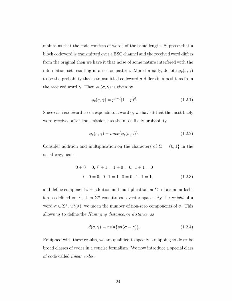
maintains that the code consists of words of the same length. Suppose that a
block codeword is transmitted over a BSC channel and the received word differs
from the original then we have it that noise of some nature interfered with the
information set resulting in an error pattern. More formally, denote φp(σ, γ)
to be the probabilty that a transmitted codeword σ differs in d positions from
the received word γ. Then φp(σ, γ) is given by
φp(σ, γ) = pn−d(1 − p)d. (1.2.1)
Since each codeword σ corresponds to a word γ, we have it that the most likely
word received after transmission has the most likely probability
φp(σ, γ) = max{φp(σ, γ)}. (1.2.2)
Consider addition and multiplication on the characters of Σ = {0, 1} in the
usual way, hence,
0 + 0 = 0, 0 + 1 = 1 + 0 = 0, 1 + 1 = 0
0 · 0 = 0, 0 · 1 = 1 · 0 = 0, 1 · 1 = 1, (1.2.3)
and define componentwise addition and multiplication on Σn in a similar fash-
ion as defined on Σ, then Σn constitutes a vector space. By the weight of a
word σ ∈ Σn, wt(σ), we mean the number of non-zero components of σ. This
allows us to define the Hamming distance, or distance, as
d(σ, γ) = min{wt(σ− γ)}. (1.2.4)
Equipped with these results, we are qualified to specify a mapping to describe
broad classes of codes in a concise formalism. We now introduce a special class
of code called linear codes.
24

We concern ourselves with the motivation of a certain class of code known
to elicit good error-correcting properties. While we earlier described codes
over Σn, we particularize this formalism of such a group code to a version
endowed with certain algebraic structures. Let Fq, where q is a prime power,
be a field. A block code C over Σn is linear over Fnq when we associate the
alphabet Σ with the field Fq if C is a subspace of Fnq .
A linear code C over Fnq is a subspace with dimension k if there exists a
minimal set of k vectors that generated the code, and in such case, we say C
is an [n, k, d]q code. Denote v1,v2, . . . ,vk to be the basis set of vectors that
generate C . Then, we can represent the code C by a generator matrix G over
Fk×nq . The rows of G correspond to the k linearly independent set of vectors
that generate C . In particular, C = {αG | α ∈ Fkq}.
If v = (v1, v2, . . . , vn) and w = (w1, w2, . . . , wn) are vectors in Fnq , we define
the inner product < v|w > of v and w as
< v|w > =n∑
i=0
vi · wi. (1.2.5)
Vectors v and w are orthogonal if < v|w > = 0. Given a generator matrix G
for the code C , we say that w is orthogonal to the code C if < vi|w > = 0
for all vi, i ∈ |k|. Therefore, the set of vectors orthogonal to C is called the
orthogonal complement, or dual code, of C and is denoted C⊥. Since C is a
linear subspace of dimension k, we have it that the orthogonal complement
C⊥ is also a subspace of Fnq with dimension n − k such that for v ∈ C and
w ∈ C⊥, < v|w > = 0. Let HT ∈ F(n−k)×nq be the generator matrix for
the code C⊥. Furthermore, a matrix H ∈ Fn×(n−k)q is called a parity-check
matrix for a linear code C if the columns of H generate the dual code C⊥,
and it is this matrix formalism that admits a useful approach to the task of
error-correction.
25
Let C be a linear [n, k, d]q code and u is some word in Fnq , we define the
coset of C determined by u to be the set of words v + u for v ∈ C . In
particular, the coset C + u is
C + u = {v + u | v ∈ C}. (1.2.6)
Suppose that the codeword v ∈ C is transmitted over a BSC and the word
u is received. Suppose further that the received word differs from that which
was transmitted resulting in an error pattern e = v− u. We seek an efficient
decoding scheme by choosing a word e of least weight in the coset C + u.
The use of the parity-check matrix H associated with the code C enables an
efficient procedure to determine a word e of least weight in the coset C + u.
To see this, we first note that for any received word u ∈ Fnq , the syndrome of u
is a word uH ∈ F(n−k)q . Should the syndrome uH = 0 then the received word
is a codeword in C . Alternatively, if uH 6= 0 then we can correctly identify
an error patterm e associated with the coset C + u that relates perfectly to
uH. We conclude that the codeword transmitted was most likely v = u− e.
26

Chapter 2
Quantum Error Correction
2.1 The Channel
We now consider the transmission of quantum information with respect to a
quantum noisy channel where a full continuum of noise is maintained. While
classical information can be transmitted and protected from the effects of noise
by replication, quantum information cannot be copied with perfect fidelity.
Introduced by Bennett et al. [5], quantum teleportation is an experimental
demonstration of the means by which quantum communication is made pos-
sible and purports a fundamental distinction between quantum and classical
information theory. Such distinction is maintained by the Bell-EPR correla-
tions whereby an essential nonlocality principle, described by quantum entan-
glement, is revealed. This result was demonstrated experimentally by Aspect
et al. in 1982 [1]. Quantum teleportation takes advantage of the non-local
behaviour of quantum mechanics by treating quantum entanglement as an in-
formation resource. The first complete transmission of quantum information
was performed by Nielsen et al. [66] in 1998.
The Church-Turing Principle [24] maintains that it is impossible to trans-
mit quantum information by implementing a classical computation. Bennett
27
et al. [5] introduced quantum teleportation to overcome this limitation by
developing a quantum algorithm that describes a complete communication
transmission of quantum information.
Given an arbitrary finite alphabet Σ of cardinality d, we process quantum
information by specifying a state description of a finite dimension quantum
space. In particular, the state description of the Hilbert space Cd. While the
state of an Σ-dimensional Hilbert space can be more generally expressed as a
linear combination of basis states |ψi〉, we write each orthonormal basis state
of the d-dimensional Hilbert space Cd to correspond with an element of Zd. In
this context the basis {|0〉 , |1〉 , . . . , |d− 1〉} is referred to as the computational
basis. Therefore, a state |ψ〉 of Cd is given by
|ψ〉 =d−1∑
i=0
αi |i〉 , (2.1.1)
where αi ∈ C and∑d−1
i=0 |αi|2 = 1. A qudit describes a state in the Hilbert
space Cd. The state space of an n-qudit state is the tensor product of the
basis states of the single system Cd, writtenHn = (Cd)⊗n, with corresponding
orthonormal basis states given by
|i1〉 ⊗ |i2〉 ⊗ · · · ⊗ |in〉 = |i1i2 . . . in〉 , (2.1.2)
where ij ∈ Zd. The general state of a qudit in the Hilbert space Hn is then
written
|ψ〉 =∑
(i1i2...in) ∈ Znd
α(i1i2...in) |i1i2 . . . in〉 , (2.1.3)
where α(i1i2 ...in) ∈ C and∑|α(i1i2...in)|2 = 1.
Quantum teleportation describes how two parties, A and B, process and
communicate quantum information in a manner secure from the effects of error.
28

zF
X
|βAB〉
|A〉
|B〉
Figure 2.1: Generalised Bell State.
Suppose A wishes to communicate the state |ψ〉 then the goal of teleportation
is to transmit that particular quantum information state to B. Further suppose
that A prepares the qudit |A〉 where |A〉 ∈ {|0〉 , |1〉 , . . . , |d− 1〉}. Similarly,
B prepares the qudit |B〉 where |B〉 ∈ {|0〉 , |1〉 , . . . , |d− 1〉}. In order to
achieve teleportation, A must interact the information state |ψ〉 with a two
qudit entangled state, |βAB〉. The entangled state |βAB〉 is called a generalised
Bell state whereby A and B each possess one qudit of this two qudit state. To
construct a generalised Bell state |βAB〉, we first apply the Fourier transform
F⊗I to the qudit |A〉. This acts on basis states |j〉 |k〉 as follows (F⊗I) |j〉 |k〉 =
1√d
∑di=0 ω
ij |i〉 |k〉 where ω is a primitive dth root of unity in C such that
ωd = 1 and ωt 6= 1 for all 0 < t < d. Secondly, we follow the Fourier transform
by the Controlled-NOT operation given by |k〉 |l〉 7→ |k〉 |l+ k (mod d)〉 for all
basis states |k〉 |l〉 which maps the two qudit state accordingly. Consequently,
any pair of qudits |A〉 |B〉 from the d2 computational basis states of Cd ⊗Cd
generate a generalised Bell state. In particular, applying the Fourier transform
29

to the first half of the pair of qudit states |A〉 |B〉, we obtain,(
1√d
d−1∑
i=0
d∑
j=0
d−1∑
x=0
ωix |x〉 |j〉 〈i| 〈j|)|A〉 |B〉
=1√d
d−1∑
i=0
d−1∑
j=0
d−1∑
x=0
ωix |x〉 |j〉 〈i|A〉〈j|B〉
=1√d
d−1∑
x=0
ωAx |x〉 |B〉 . (2.1.4)
The action of the Controlled-NOT operator on resulting state (2.1.4) completes
the generalised Bell state construction(
d−1∑
k=0
d−1∑
l=0
|k〉 |l + k〉 〈k| 〈l|)
1√d
d−1∑
x=0
ωAx |x〉 |B〉
=1√d
d−1∑
l=0
d−1∑
k=0
d−1∑
x=0
ωAx |k〉 |l + k〉 〈k|x〉〈l|B〉
=1√d
d−1∑
x=0
ωAx |x〉 |B + x〉
= |βAB〉 . (2.1.5)
Since the Bell pair is an entangled state [60], any operator acting on the first
qudit held by A influences the state of the second qudit held by B. This con-
dition permits the teleportation of the quantum information state |ψ〉 between
parties A and B when A interacts |ψ〉 with the first half of the generalised
Bell pair (2.1.5). To negate the effects of the Bell state transformations on
|ψ〉, thereby allowing the teleportation of |ψ〉, A transforms |ψ〉 by apply-
ing the inverse of the generalised Controlled-NOT operator for qudit states
which is then followed by an application of the inverse Fourier transform.
Now, the Fourier transform is unitary so its inverse is its adjoint, and the
inverse of the generalised Controlled-NOT operation has its action defined as
|k〉 |l〉 7→ |k〉 |l− k (mod d)〉.
30
X−1
v zz
F
M2
M1
X−B−M2 Z−A−M1
|βAB〉
|ψ〉
|ψ〉
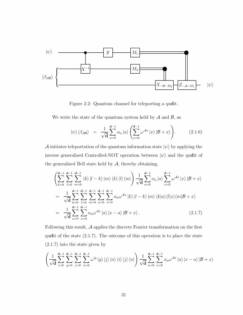
Figure 2.2: Quantum channel for teleporting a qudit.
We write the state of the quantum system held by A and B, as
|ψ〉 |βAB〉 =1√d
d−1∑
a=0
αa |a〉(
d−1∑
x=0
ωAx |x〉 |B + x〉). (2.1.6)
A initiates teleportation of the quantum information state |ψ〉 by applying the
inverse generalised Controlled-NOT operation between |ψ〉 and the qudit of
the generalised Bell state held by A, thereby obtaining,
(d−1∑
k=0
d−1∑
l=0
d−1∑
m=0
|k〉 |l − k〉 |m〉 〈k| 〈l| 〈m|)
1√d
d−1∑
a=0
αa |a〉d−1∑
x=0
ωAx |x〉 |B + x〉
=1√d
d−1∑
k=0
d−1∑
l=0
d−1∑
m=0
d−1∑
a=0
d−1∑
x=0
αaωAx |k〉 |l − k〉 |m〉 〈k|a〉〈l|x〉〈m|B + x〉
=1√d
d−1∑
a=0
d−1∑
x=0
αaωAx |a〉 |x− a〉 |B + x〉 . (2.1.7)
Following this result, A applies the discrete Fourier transformation on the first
qudit of the state (2.1.7). The outcome of this operation is to place the state
(2.1.7) into the state given by
(1√d
d−1∑
i=0
d−1∑
y=0
d−1∑
j=0
d−1∑
n=0
ωiy |y〉 |j〉 |n〉 〈i| 〈j| 〈n|)
1√d
d−1∑
a=0
d−1∑
x=0
αaωAx |a〉 |x− a〉 |B + x〉
31

=1
d
d−1∑
i=0
d−1∑
y=0
d−1∑
j=0
d−1∑
n=0
d−1∑
a=0
d−1∑
x=0
αaωiyωAx |y〉 |j〉 |n〉 〈i|a〉〈j|x− a〉〈n|B + x〉
=1
d
d−1∑
y=0
d−1∑
a=0
d−1∑
x=0
αaωayωAx |y〉 |x− a〉 |B + x〉
=1
d
d−1∑
y=0
d−1∑
a=0
d−1∑
x=0
d−1∑
z=0
αaωayωAx |y〉 |z〉 〈z|x− a〉 |B + x〉
=1
d
d−1∑
y=0
d−1∑
a=0
d−1∑
z=0
αaωayωA(z+a) |y〉 |z〉 |B + z + a〉
=1
d
d−1∑
y=0
d−1∑
z=0
ωAz |y〉 |z〉(
d−1∑
a=0
αaωa(y+A) |B + z + a〉
). (2.1.8)
The qudit of the generalised Bell state held by B is transformed into the state∑d−1
a=0 αaωa(y+A) |B + z + a〉. Thus A has teleported a quantum information
state |ψ′〉 to B, however, it has been subjected to error over the channel
and therefore B receives∑d−1
a=0 αaωa(y+A) |B + z + a〉 instead of
∑d−1a=0 αa |a〉.
A measurement projection onto the computational basis state of Cd ⊗ Cd
is performed by A on the first and second qudit of the state of the quan-
tum system (2.1.8) which yields two classical numbers. Simultaneously, the
third qudit of the state of the system (2.1.8) teleported to B collapses to a
post-measurement state that is dependent upon the measurement outcome
obtained by A. Let M1,M2 be two classical numbers corresponding to the
resulting states |M1〉 |M2〉. Then the state of the qudit held by B is given
by∑d−1
a=0 αaω(A+M1)a |B +M2 + a〉. The set M1,M2 is transferred by classical
means to B, where upon delivery B learns which of the generalised Pauli op-
erators are required to correct the effect of the error. In particular, B applies
the operators
X−B−M2 =
d−1∑
x=0
|x− B −M2〉 〈x|
32
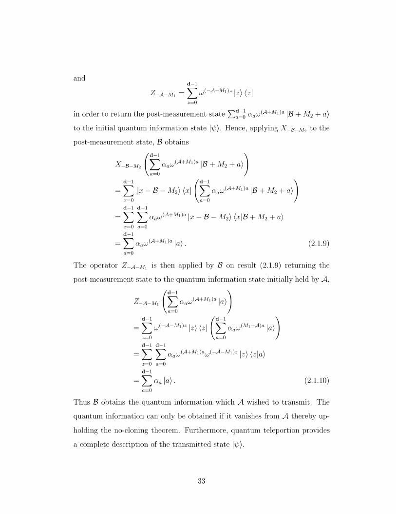
and
Z−A−M1 =d−1∑
z=0
ω(−A−M1)z |z〉 〈z|
in order to return the post-measurement state∑d−1
a=0 αaω(A+M1)a |B +M2 + a〉
to the initial quantum information state |ψ〉. Hence, applying X−B−M2 to the
post-measurement state, B obtains
X−B−M2
(d−1∑
a=0
αaω(A+M1)a |B +M2 + a〉
)
=d−1∑
x=0
|x− B −M2〉 〈x|(
d−1∑
a=0
αaω(A+M1)a |B +M2 + a〉
)
=d−1∑
x=0
d−1∑
a=0
αaω(A+M1)a |x− B −M2〉 〈x|B +M2 + a〉
=
d−1∑
a=0
αaω(A+M1)a |a〉 . (2.1.9)
The operator Z−A−M1 is then applied by B on result (2.1.9) returning the
post-measurement state to the quantum information state initially held by A,
Z−A−M1
(d−1∑
a=0
αaω(A+M1)a |a〉
)
=d−1∑
z=0
ω(−A−M1)z |z〉 〈z|(
d−1∑
a=0
αaω(M1+A)a |a〉
)
=d−1∑
z=0
d−1∑
a=0
αaω(A+M1)aω(−A−M1)z |z〉 〈z|a〉
=d−1∑
a=0
αa |a〉 . (2.1.10)
Thus B obtains the quantum information which A wished to transmit. The
quantum information can only be obtained if it vanishes from A thereby up-
holding the no-cloning theorem. Furthermore, quantum teleportion provides
a complete description of the transmitted state |ψ〉.
33
2.2 An Error Model
The challenge of quantum information processing is to elicit a reliable form
of communication and to maintain such a form in the presence of quantum
noise. Noise is a characteristic of the environment associated with an in-
formation state and is a property of an open quantum system that subjects
an information state to unwanted interactions with the elements of the en-
vironment during teleportation. It is inevitable that the communication of
an information state will cause interactions with the environment. However,
prolonged contact between the information state and environment is soon to
suffer in entanglement that degrades the information state. This process is
called decoherence. Any strategy to stabilize quantum computations from the
effects of noise will ultimately be required to deal with both the problems
of decoherence and unitary imperfections of channel communication. Thus,
to understand the fundamentals of noise propagation is to understand the
formalism of a model that explains it.
Given a qudit information state |ψ〉 =∑d−1
i=0 αi |i〉 of the Hilbert space Cd,
let us consider an adjoined environment space |E〉 endowed with an orthonor-
mal basis of dimension d2. We suppose that both the state space of the qudit
and the corresponding environment space are initially independent systems.
The joint state of the systems |ψ〉 and |E〉 is then |ψ〉 ⊗ |E〉 and its dynamics
may be characterised when we further suppose that the joint system evolves
according to some unitary operation. Given a unitary operation U , we write
interaction of each basis qudit with the environment under U as
U(|i〉 ⊗ |E〉) =d−1∑
l=0
γ−i+l,−i(|i+ l〉 ⊗ |e−i+l,−i〉)
34

=d−1∑
l=0
|i+ l〉 ⊗ γ−i+l,−i |e−i+l,−i〉 , (2.2.1)
for i ∈ {0, . . . ,d − 1}. By linearity of U , the dynamics of the joint system
|ψ〉 ⊗ |E〉 is then
U(|ψ〉 ⊗ |E〉) = U
((d−1∑
i=0
αi |i〉)⊗ |E〉
)= U
(d−1∑
i=0
αi(|i〉 ⊗ |E〉))
=d−1∑
i=0
αiU(|i〉 ⊗ |E〉) =d−1∑
i=0
d−1∑
l=0
αi |i+ l〉 ⊗ γ−i+l,−i |e−i+l,−i〉 . (2.2.2)
Since 1d
∑d−1z=0 ω
zk = 1 if z = 0 and vanishes otherwise then equation (2.2.2)
may be written as
1
d
d−1∑
i=0
d−1∑
l=0
(αi |i+ l〉 ⊗
(d−1∑
z=0
d−1∑
k=0
ωzkγ−i+l+z,−i+z |e−i+l+z,−i+z 〉
))
=1
d
d−1∑
i=0
d−1∑
l=0
d−1∑
k=0
(αi |i+ l〉 ⊗
(d−1∑
z=0
ωzkγ−i+l+z,−i+z |e−i+l+z,−i+z 〉))
=1
d
d−1∑
l=0
d−1∑
k=0
(d−1∑
i=0
(αi |i+ l〉 ⊗
(d−1∑
z=0
ωzkγ−i+l+z,−i+z |e−i+l+z,−i+z 〉)))
=1
d
d−1∑
l=0
d−1∑
k=0
(d−1∑
i=0
(ωikαi |i+ l〉 ⊗
(d−1∑
z=0
ω−ikωzkγ−i+l+z,−i+z |e−i+l+z,−i+z 〉
)))
=1
d
d−1∑
l=0
d−1∑
k=0
(d−1∑
i=0
(ωikαi |i+ l〉 ⊗
(d−1∑
z′=0
ωz′kγz′+l,z′ |ez′+l,z′ 〉)))
=1
d
d−1∑
l=0
d−1∑
k=0
((d−1∑
i=0
ωikαi |i+ l〉)⊗(
d−1∑
z′=0
ωz′kγz′+l,z′ |ez′+l,z′ 〉))
. (2.2.3)
An outer product representation describes the set of errors that act on the
joint quantum state under U . The operator X1 =∑d−1
i=0 |i+ 1〉 〈i| maps
αi |i〉 to αi |i+ 1〉 for i ∈ {|0〉 , . . . , |d− 1〉}, and thus maps∑d−1
i=0 αi |i〉 to∑d−1
i=0 αi |i+ 1〉. Similarly, Z1 =∑d−1
i=0 ωi |i〉 〈i| maps αi |i〉 to ωiαi |i〉 and cor-
respondingly maps∑d−1
i=0 αi |i〉 to∑d−1
i=0 ωiαi |i〉. Both X1 and Z1 are called
35

the Weyl Pair [96]. Consequently, the action of U on |ψ〉 ⊗ |E〉 is described
by the set of operators XlZk =∑d−1
i=0 ωik |i+ l〉 〈i| , (l, k) ∈ Zd × Zd,
d−1∑
l=0
d−1∑
k=0
((d−1∑
i=0
ωikαi |i+ l〉)⊗ 1
d
(d−1∑
z′=0
ωz′kγz′+l,z′ |ez′+l,z′〉))
=d−1∑
l=0
d−1∑
k=0
XlZk |ψ〉 ⊗ γlk |elk〉 . (2.2.4)
Thus, to correctly specify an error model that describes the action of a unitary
operator U on the joint space |ψ〉 ⊗ |E〉, it is necessary that the environment
|E〉, associated with an information state in Cd, be a Hilbert space of dimen-
sion d2. Following the action of U on the joint system, a measurement on the
environment is performed with respect to the basis |emn〉 , (m,n) ∈ Zd × Zd
to diagnose the introduced error in result (2.2.4). Therefore, equation (2.2.4)
provides the conceptual foundation of quantum error correction. Measure-
ments taken in the environment basis initiate the correction step (XmZn)−1 =
Z(−n mod d)X(−m mod d).
The depolarization channel is a well investigated error model, see [60], and
references therein, and it is the error model with which we concern ourselves.
We adapt its qubit form to cater for qudits so that the effects of noise as those
modelled by equation (2.2.4) can be explained. In particular, we have it that
there is a 1 − (d2−1)p
d2 probability that |ψ〉 will not suffer the effects of noise
and a pd2 probability that any given error will occur. The depolarizing channel
for qudits is therefore represented as
U(|ψ〉 ⊗ |E〉) 7→√
1 − (d2 − 1)p
d2 |ψ〉 ⊗ |eX0Z0〉+√
p
d2
∑
(k,l)\(0,0)∈ Zd×Zd
XlZk |ψ〉 ⊗ |eXlZk〉
. (2.2.5)
36

In general, we consider the case where 1 − (d2−1)p
d2 > pd2 , and as such the
probability of an error operator decreases exponentially with weight [2]. Con-
sequently, good n-qudit error-correcting codes are those for which all errors of
weight ≤ p
d2n can be corrected. It is for this reason that the rationale for error
analysis is guided by the necessity to detect and error correct error operators
up to a given weight [2].
2.3 Definition and basic properties
The process of quantum error detection and correction raises difficulties not
evident in the classical analogue. Firstly, the coding theorist must contend
with an extra class of error, phase errors, and any subsequent linear combi-
nations with qudit flip errors that are introduced by the environment during
information transmission. Secondly, information transmission causes commu-
nication signals to become attenuated which is primarily due to the physical
capabilities of the hardware used. Consequently, the likelihood of errors occur-
ring during transmission may increase. In particular, the 10−4 threshold level
is widely assumed to be the fault-tolerant threshold for both environmentally
induced and systematic errors. More rigorous bounds recently calculated sug-
gest that this threshold could be closer to 10−5 [85], and references therein.
For what follows, it is worth noting that a robust CNOT gate could operate
at close to the 10−7 level, a level well within more rigorous threshold bounds.
Furthermore, for systems whose Hamiltonian is unclear, the CNOT operating
at the 10−7 level represents an important result as it suggests that operating
the CNOT gate in this way can ensure that the error rate remains below the
fault-tolerant error threshold [69, 85]. Finally, the no-cloning theorem main-
tains that it is impossible to generate copies of an unknown quantum state.
37

Classical error correction enables reliable communication by the process of
data replication. However, measurements that allow classical information to
be obtained cause the collapse of a quantum state thereby destroying the quan-
tum information content. Quantum error detection and correction schemes do
exist despite these difficulties.
A quantum code C consists of an encoding function E from the Hilbert
space Hk = (Cd)⊗k ≡ Cdkto the Hilbert space Hn = (Cd)⊗n ≡ Cdn
, where k
and n are integers and k < n. We define the codewords of a quantum code to
be those states contained in the image of E, Im(E). The length of the code is
given by n, while k denotes the number of encoded message qudits, or logical
qudits, of the code. The extra n− k qudits introduce additional information
that allows the logical qudits to be stored in a redundant manner where such
redundancy can be used to detect transmission errors. A code C is a quantum
n, kd
code over Cd if it is a subspace of dimension dk in the Hilbert space
Hn.
An error operator E acting on a qudit state can be written as a linear
combination of E = {XlZk : (l, k) ∈ Zd × Zd}. The generalised Pauli group,
G1 is a group has order d4 generated by E and τI with center ζ(G1) = 〈τI〉.
For an n-qudit system, any operator E of the group G⊗n1 can be written as
E = τα(Xl1Zk1)⊗ (Xl2Zk2)⊗ · · · ⊗ (XlnZkn ), (2.3.1)
where α ∈ {0, . . . ,d − 1} and ((l1, k1), (l2, k2), . . . , (ln, kn)) ∈ Znd × Zn
d. The
weight of the error E, wt(E), in E⊗n is the number of pairs (li, ki) for which
li and ki are not both zero.
Let |ψ〉 ∈ C be a codeword that is transmitted across a noisy quantum
channel. Thus |ψ〉 has the expansion∑d−1
k=0
∑d−1l=0 XlZk |ψ〉 ⊗ |eXlZk
〉. This re-
sult provides a conceptual starting point for which a quantum error-correcting
38

code can be explained. Let {ψ1, . . . , ψn−k} be an orthogonal basis for C and
write {E} = {E1, . . . , Ed2}. To detect an error E in E in the computational
basis of C, we require that the state E |ψi〉 be orthogonal from all |ψj〉, hence,
〈ψj |E|ψi〉 = 0. To correct an error, we require that the action of error El on
|ψi〉 be distinct from the action of Ek, for k 6= l , on |ψj〉. Hence, a necessary
condition for quantum error-correcting is given by 〈ψj |E†kEl|ψi〉 = 0 for i 6= j
and for all Ek, El ∈ E. If this condition were not satisfied for i 6= j and k 6= l,
we have |ψz〉 = El |ψi〉 = Ek |ψj〉. Suppose |ψz〉 is a received word then it
would not be possible to determine the original codeword transmitted since
the distinguishability of the orthogonal codewords is destroyed. To see that
this necessary condition is also sufficient, let us assume that Ek |ψj〉 is distinct
from El |ψi〉, for i 6= j and k 6= l, and construct a decoding function D(|ψ〉).
Then there is a unique |ψi〉 ∈ C and Ei(z) ∈ E for which Ei(z)=l |ψi〉 = |ψz〉 is
true. Thus we can decode |ψz〉 by defining |ψi〉 = D(|ψz〉).
We now give a formal treatment of the quantum error-correcting code
conditions. The quantum error correcting conditions are a set of equations
which can be checked to determine whether a quantum code protects against
a particular type of noise from the environment. The set of error-correcting
conditions for quantum error-correcting codes were introduced by Knill and
Laflamme [52]. These conditions for qubit error-correcting codes were dis-
cussed further in Nielsen and Chuang [60]. We adapt the proof of Nielsen and
Chuang [60] and consider the formulation of these conditions with respect to
quantum basis states instead of density matrices. We also cater for quantum
error-correcting codes over larger dimensions.
Theorem 1. [52] Let C be a subspace of the Hilbert space H. Then C is a
quantum error-correcting code for the error operators E = {E1, . . . , Ed2} if
39

and only if there exists αl,k ∈ C such that, for all |ψi〉 , |ψj〉 ∈ C and Ek, El in
E,
〈ψj|E†kEl |ψi〉 = αl,kδij. (2.3.2)
Proof : It is necessary that
〈ψj|E†kEl |ψi〉 = 0, (2.3.3)
for i 6= j, otherwise the action of an error operator would destroy the distin-
guishability of orthogonal codewords. The non-trivial content αl,k of condition
(2.3.2) presents a stronger argument than the necessary condition, in that the
assumed Hermition matrix α with entries αl,k = 〈ψi|E†kEl |ψi〉 does not de-
pend on i. This argument is qualified since the action of any error mapping
must take orthogonal codewords to orthogonal states as any projective mea-
surement on the error space would reveal information thereby disturbing the
state of the system. Furthermore, suppose F is a quantum operation with op-
erations {Fm} which are linear combinations of the {Ek, k ∈ {1, . . . ,d2}, that
is, Fm =∑
k βm,kEk for some matrix βm,k of complex numbers. The action of
the error operators Fm on a code basis state is given by
|ψi〉 ⊗ |E〉 7→∑
m
Fm |ψi〉 ⊗ |em〉 (2.3.4)
where the states |em〉 denote an orthonormal basis for the environment. Re-
covery is accomplished if there exist an operator R with operation {Rn} such
that
∑
n
R†nRn = I (2.3.5)
and
∑
m,n
RnFm |ψi〉 ⊗ |em,n〉 ∝ |ψi〉 ⊗ |em,n〉 . (2.3.6)
40

Since |em,n〉 does not depend on i, it follows that
RnFm |ψi〉 = λm,n |ψi〉 , (2.3.7)
λm,n ∈ C. Therefore, {RnFm} acts trivally on the code space∑
i |ψi〉. With
the assumption of completeness, that is condition (2.3.5), on {Rn}, we have it
that
F †uFm |ψi〉 = F †
u
(∑
n
R†nRn
)Fm |ψi〉
=∑
n
λ∗u,nλn,m |ψi〉 , (2.3.8)
thereby illustrating the trival action of F †uFm on the basis states {|ψi〉}. Con-
sidering
〈ψj|F †uFm |ψi〉 = αu,mδij, (2.3.9)
where αu,m =∑
n λ∗u,nλn,m, the error correcting condition follows.
To show that condition (2.3.2) is also sufficient, we need to illustrate that
the recovery operator R can be explicitly constructed. By assumption, we
have it that α is a Hermitian matrix and can therefore be diagonalised,
〈ψj|F †uFm |ψi〉 = αmδumδij, (2.3.10)
where∑
m αm = 1 follows from the normalisation condition. For each n with
Rn 6= 0 make the correspondence
Rn =1√αn
∑|ψi〉 〈ψi|F †
n. (2.3.11)
The set of recovery operators Rn satisify the normalisation condition since∑
n R†nRn =
∑n,i
1αnFn |ψi〉 〈ψi|F †
n. The action of Rn on Fm |ψi〉 is given by
41

√αnδmn |ψi〉. To show that this correction procedure is legitimate, we have it
that
∑
n,m
RnFm |ψi〉 ⊗ |em,n〉 = |ψi〉 ⊗(∑
n
√αn
)|em,n〉 , (2.3.12)
thus we can recover the code space from the effects of error.
The distance of the code C is the minimal weight of E in En such that
condition (2.3.2) does not hold. An n, kd
code C with distance d is called
an n, k, dd
quantum code.
Theorem 2. If a quantum code C corrects errors of weight ≤ < then C is
2< error-detecting. If C detects errors of weight ≤ = then C is b=/2c error-
correcting.
Proof : For all m with wt(Em) ≤ 2<, write Em = E†kEl such that wt(E†
k),
wt(El) ≤ <. Then 〈ψj|Em|ψi〉 = 〈ψj|E†kEl|ψi〉 = αl,kδij. Thus, C is 2< error
detecting where αm = αl,k.
For k, l with wt(E†k), wt(El) ≤ b=/2c then E†
kEl has weight≤ =. The prod-
uct E†kEl has support ωk,lEk,l and therefore 〈ψj |E†
kEl|ψi〉 = ωk,l〈ψj |Ek,l|ψi〉 =
ωk,lαl,kδij since C is= error detecting. Writing α′l,k = ωk,lαl,k, then 〈ψj|E†
kEl|ψi〉
= α′l,kδij and C is therefore b=/2c error-correcting.
Theorem 3. An n, k, dd
quantum code detects errors of weight ≤ d− 1 and
corrects errors of weight ≤ b(d − 1)/2c.
Proof : Since C has distance d there exists an error Em of weight d−1 such
that 〈ψj|Em|ψi〉 = αmδij, thereby, illustrating C to be d − 1 error-detecting.
Writing Em as the product of pairs E†kEl with wt(E†
k) and wt(El) ≤ b(d−1)/2c
then 〈ψj|Em|ψi〉 = 〈ψj|E†kEl|ψi〉 = αl,kδij and C is b(d−1)/2c error-correcting.
42

2.4 A Quantum Qudit Code
Quantum error correction was first demonstrated by Steane [83] and by Calder-
bank and Shor [14]. A group-theoretic formalism was introduced by Gottes-
man [31] and Calderbank et al. [12] and led to the discovery of many more
quantum error correcting codes. Since then the theory of quantum error cor-
rection has matured remarkably quickly.
Let us consider information transmission over a channel that protects a
single qudit against error. Introduced by Shor [79], the quantum 9, 12
code
illustrates that quantum error-correction is possible. The code proposed by
Shor is a quantum bit generalisation of the classical 3-bit repetition code, and
is characterised by specifying two basis states for the code subspace. These
basis states are referred to as |0〉, the logical 0, and |1〉, the logical 1, and are
written
|0〉 = [1√2(|000〉 + |111〉)]⊗3 (2.4.1)
|1〉 = [1√2(|000〉 − |111〉)]⊗3 (2.4.2)
Since the encoded qubit is written in the guise of entanglement, the informa-
tion content is dispersed among the nine qubits where it is then said to be
encoded nonlocally with protection from decoherence ensured because of this
nonlocal property of encoded information.
We seek to extend error correction beyond the binary setting it was original
envisaged and to which most results are derived. Suppose we wish to protect
an unknown single quantum state of Cd that has been prepared as
|ψ〉 =d−1∑
i=0
αi |i〉 (2.4.3)
for αi ∈ C and∑d−1
i=0 |αi|2 = 1.
43
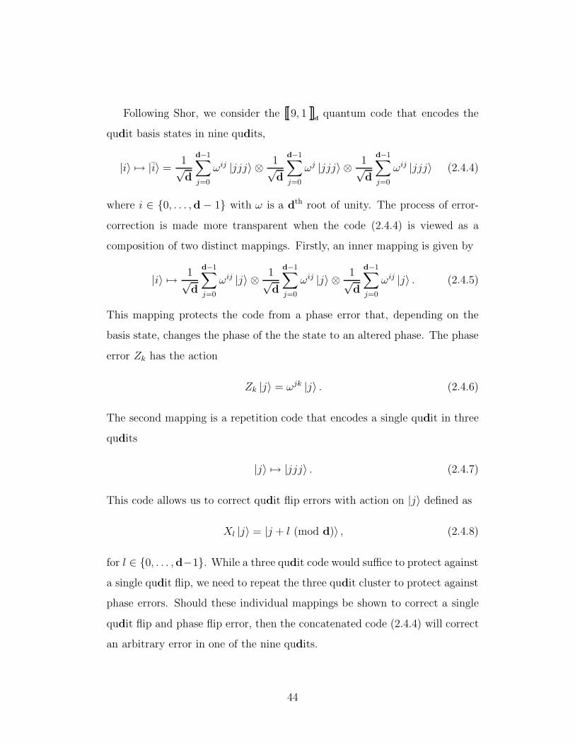
Following Shor, we consider the 9, 1d
quantum code that encodes the
qudit basis states in nine qudits,
|i〉 7→ |i〉 =1√d
d−1∑
j=0
ωij |jjj〉 ⊗ 1√d
d−1∑
j=0
ωj |jjj〉 ⊗ 1√d
d−1∑
j=0
ωij |jjj〉 (2.4.4)
where i ∈ {0, . . . ,d − 1} with ω is a dth root of unity. The process of error-
correction is made more transparent when the code (2.4.4) is viewed as a
composition of two distinct mappings. Firstly, an inner mapping is given by
|i〉 7→ 1√d
d−1∑
j=0
ωij |j〉 ⊗ 1√d
d−1∑
j=0
ωij |j〉 ⊗ 1√d
d−1∑
j=0
ωij |j〉 . (2.4.5)
This mapping protects the code from a phase error that, depending on the
basis state, changes the phase of the the state to an altered phase. The phase
error Zk has the action
Zk |j〉 = ωjk |j〉 . (2.4.6)
The second mapping is a repetition code that encodes a single qudit in three
qudits
|j〉 7→ |jjj〉 . (2.4.7)
This code allows us to correct qudit flip errors with action on |j〉 defined as
Xl |j〉 = |j + l (mod d)〉 , (2.4.8)
for l ∈ {0, . . . ,d−1}. While a three qudit code would suffice to protect against
a single qudit flip, we need to repeat the three qudit cluster to protect against
phase errors. Should these individual mappings be shown to correct a single
qudit flip and phase flip error, then the concatenated code (2.4.4) will correct
an arbitrary error in one of the nine qudits.
44

2.5 Qudit Error Correction
Error-correction has its foundations in classical theory, however, considering
such thought within the quantum setting presents difficulties not evident in
the classical setting. The classical majority voting scheme requires a mea-
surement of bits to correct errors. However, a projective measurement taken
on the information state will collapse the superposition leading to the loss of
information. Furthermore, we note that where once we protected information
by making copies of the information, the no-cloning theorem [60] maintains
the quantum information cannot be copied. We take Shor’s quantum 9, 12
binary repetition code [79] and generalise it to the qudit setting as given in
equation 2.4.4. We look at how error-correction on such a code may be ad-
dressed with respect to two procedures. The first procedure requires the use of
non-demolition measurements [22] to construct the error syndrome. Recently,
Lu and Marinescua [54] have provided a nondemolition algorithm argument
that describes an error-correction procedure for use with the Steane code. The
second procedure views error-correction and syndrome diagnosis with respect
to a projective formalism.
A single qudit may be encoded in three qudits, and the corresponding
superposition state is written
d−1∑
i=0
αi |i〉 7→d−1∑
i=0
αi |iii〉. (2.5.1)
For a given three qudit state |a, b, c〉, we have it that any measurement per-
formed directly on the states leads to a collapse of the superposition state. To
avoid such an outcome, a quantum nondemolition measurement [22] is instead
performed on pairs of qudits. Quantum nondemolition measurements were
originally envisaged to be a measurement of a ”total” photon number which
45

would determine whether quantum jumps due to loss had occurred while still
preserving the superposition state [22]. Further, quantum error-correction re-
quires nondemolition measurements of the error syndrome in order to preserve
the quantum state [54]. Such nondemolition measurements allows us to con-
struct the error syndrome and on examining the syndrome an error correcting
procedure should be able to decide whether; an error has occurred for which
no correcting action is take, one error has occurred for which we apply the
corresponding Pauli transformation to the state in error, or lastly, if two or
more errors have occurred for which a quantum error-correcting code capable
of correcting a single error will fail. We now describe an alorithm based on
the qudit repetition code. Without loss of generality, let us consider a qudit
flip Xl acting on the first qudit of the superposition,
d−1∑
j=0
αj |jjj〉 7→ (Xl ⊗ I ⊗ I)d−1∑
j=0
|jjj〉
=d−1∑
j=0
αj |j + ljj〉. (2.5.2)
Figure 2.3 describes the circuit that returns one of the syndrome’s values
(a + b). A similar argument returns the remaining syndrome values. The
returned values (b + c), (a + c) and (a + b), with addition in Zd, constitute
a syndrome that reveals the error location. Figure 2.3 consists of a pair of
CNOT gates. Both CNOT gates target the ancilla qudit prepared in the
state |0〉 where it is necessary that measurement of the ancilla should not
influence the superposition state of the system. A nondemolition measurement
performed on the state |j + ljj〉 returns the syndrome (b + c, a + c, a + b) =
(2j, 2j + l, 2j + l). Since (b + c) = 2j is the differing value of the syndrome,
then the revealed error location is qudit position one. A unique solution for j
can be found from (b+ c) = 2j when d > 2 and d 6= 0 (mod2) and l is given
46

|0〉
|b〉
|a〉
|c〉
a+ bm m
tt
Figure 2.3: Non-demolition measurement circuit.
by (a + c) − (b + c). Recovery of initial qudit state is achieved by applying
(X−l ⊗ I ⊗ I) to∑d−1
j=0 |j + ljj〉.
As an alternative to error-corection via a nondemoltion preocedure, we may
consider error-correction by describing a syndrome diagnosis under a projec-
tive formalism. Syndrome diagnosis via projective measurements on qubit
repetition code is discussed in Nielsen and Chuang [60]. In respect of this, and
to generalise, we have it that the projector M0 =∑d−1
j=0 |jjj〉 〈jjj| measures
no error having taken place on the logical qudit state by returning a value of
one. Similarly, the measurements M1 =∑d−1
i=0
∑d−1j=0 |j + ijj〉 〈j + ijj|, M2 =
∑d−1i=0
∑d−1j=0 |jj + ij〉 〈jj + ij|, and M3 =
∑d−1i=0
∑d−1j=0 |jjj + i〉 〈jjj + i| re-
turn a value of one, if the logical codeword has the qudit flip error, Xi, i ∈
{1, . . . ,d−1}, in position one, two, or three, respectively, of the logical qudit.
Suppose also that an error flips that state of the first qudit so that the cor-
rupted state is |ψ〉 =∑d−1
j=0 αj |j + ljj〉. Now note that 〈ψ|M1|ψ〉 = 1 in this
case. Furthermore, the projective measurement does not cause that state to
change; it remains the same both before and after the measurement. Thus,
the syndrome contains only information about what error has occurred and
does not provide any information about the state itself. A repeat application
of X1 at the error location, with the identity elsewhere, on the logical state
followed by the projector M0 until the action of M0 equals unity completes
47

the recovery.
Having protected the code against any possible qudit flip error, we follow in
similar fashion to protect against phase errors. Therefore, we encode a single
qudit using nine qudits according to
|i〉 7→ 13√
d
d−1∑
j=0
ωkj |jjj〉 ⊗d−1∑
j=0
ωkj |jjj〉 ⊗d−1∑
j=0
ωkj |jjj〉 (2.5.3)
Suppose that a phase error occurs on the first qudit, then the basis state are
written as
(Zk′ ⊗ I ⊗ · · · ⊗ I) 13√
d
d−1∑
j=0
ωkj |jjj〉 ⊗d−1∑
j=0
ωkj |jjj〉 ⊗d−1∑
j=0
ωkj |jjj〉
=1
3√
d
d−1∑
j=0
ω(k+k′)j |jjj〉 ⊗d−1∑
j=0
ωkj |jjj〉 ⊗d−1∑
j=0
ωkj |jjj〉 (2.5.4)
for some k′ ∈ {0, ...,d− 1}. The introduction of the error causes the relative
sign of |jjj〉 in the first cluster of qudits to change. As we do not measure
the phase directly since such a measurement would destroy the superposition
state then correction with respect to a non-demolition measurement is sought.
The relative phase degree of pairs of the three qudit clusters A,B,C motivate
such a syndrome, in particular, (B + C,A+ C,A+B). As in the case of the
qudit-flip error, we determine the damaged cluster and error by comparing
the results of the non-demolition measurement. The quantum circuit imple-
mented in the qudit flip case to generate a non-demolition syndrome may be
used to generate a similar type of syndrome to detect a qudit phase error.
Alternatively, a circuit known as the Toffoli circuit can be implemented to
give a similar outcome [86]. An n bit Toffoli gate, θ(n) is defined as
(x1, x2, ..., xn−1, y)→ (x1, x2, ..., xn−1, y ⊕ x1x2...xn−1) (2.5.5)
48

The Toffoli gate allows us to take the product of the clusters’ relative phase.
The recorded ancilla, y, provides no individual information of a particular
cluster’s relative phase but rather it gives a combined measurement. The
non-demolition syndrome associated with a Toffoli circuit is given by
(BC,AC,AB) (2.5.6)
A particular value of the non-demolition syndrome, BC, is the result of imple-
menting the mapping
(ωkj |j〉 , ωkj |j〉 , |0〉)→ (ωkj |j〉 , ωkj |j〉 , |0〉 ⊕ ωkj |j〉ωkj |j〉) (2.5.7)
The returned ancilla |0〉⊕ω(2k)j |j〉, along with similar values for the remaining
elements of the syndrome permits error recovery.
While a single error XlZk acting on any one of the nine qudits will cause
no irrevocable damage, should more than one error occur then the encoded
information will be damaged. For example, if the first two qudits in a cluster
flip then we misdiagnose the error and attempt recovery by flipping the third.
Similarly, the encoded information will be damaged if phase errors occur in
two different clusters. A phase error will be introduced in a misguided attempt
at correction.
49

Chapter 3
Unitary Error Bases
The theory of quantum error correction is increasingly well understood. The
recent results of Shor and Steane marked the initial development of quantum
coding theory. Subsequently, Calderbank and Shor have shown that good
quantum codes exist and formulated their notion of quantum control codes on
classical binary group codes. Introduced by Gottesman [32] and Calderbank,
Rains, Shor, and Sloane [13], the stabilizer code is a class of quantum code and
further popularises the connection between the quantum and classical realm.
A large body of theory and practice has been developed around the stabilizer
formalism.
Teleportation was demonstrated to be an initial feature of information
processing that makes use of a correlated system between the two parties to
send quantum information in a secure manner. The means for why this is
possible in the quantum setting and impossible in a classical analogy rests
with a particular type of connection known as entanglement. Entanglement
describes the process by which quantum states can be described with reference
to each other.
The majority of publications relating to quantum coding theory are re-
stricted to the binary setting. Popular models of quantum computing such
50

as the Ion Trap, Cavity QED, and NMR require the storage of qubits for an
extended period of time and that such qubits be isolated from the environment
to reduce decoherence. In addition, quantum hardware must measure qubits
and perform controlled operations. Any successful implementation of these
models will need to meet these requirements. A research group directed at the
National Institute for Standards and Technology have made studies into how
qubits are carried by a single ion. Monroe et al. [58] have illustrated that the
quantum XOR gate can be implemented in an ion trap using a series of laser
pulses. Another model of quantum hardware makes use of nuclear magnetic
resonance (NMR) technology to prepare a maximally entangled state of three
qubits.
The role of an error model in quantum information processing is crucial to
the theory of quantum processing as it permits quantum error correction, tele-
portation, and physical demonstrations of quantum models. It is inevitable
that a system will interact with the environment and to ensure that infor-
mation is accurately processed we are required to understand the effects of
environment on information. The set of Pauli matrices for a single qubit de-
scribes an error model for the binary case of quantum information theory.
Indeed, a class of quantum code called stabilizer codes are defined as the com-
mon eigenspace of a subset of Pauli matrices thus illustrating an important
role of an error model.
Before any thoughts of scaling quantum computing and hardware to a
non-binary setting, we need to consider error operators that act on higher
dimensional quantum states. Such error bases should provide a natural ex-
tension from binary to non-binary and lead to codes over the ring of integers
modulo d.
51

3.1 Higher Dimensional Unitary Error Bases
The bit and phase flip error basis is an important prime in the theory of
quantum information. This basis has permitted the construction of a class of
quantum code that identifies the common eigenspace of an Abelian subgroup
of the well known Pauli group. The Pauli error group G1 = 〈X,Z, iI〉 contains
the set P = {I,X,Z, Y } of Pauli matrices given by
I =
(1 00 1
), X =
(0 11 0
), Z =
(1 00 −1
), Y =
(0 −ii 0
). (3.1.1)
Any matrix A in C2 can be expressed as a linear combination of the Pauli
matrices. In particular,
A =1
2(tr(A)I + tr(X†A)X + tr(Y †A)Y + tr(Z†A)Z). (3.1.2)
We concern ourselves with the generalisation of unitary error basis associated
with the Pauli group for higher dimensional quantum systems and confine our-
selves to the set errors that form a basis of Cd2since it is a well known premise
of quantum coding theory that if a code can correct a set E of errors then the
code also corrects the linear span of E [32, 65]. To motivate a description of
such a set E for higher dimensional systems, let us again consider the Pauli
group G1 = 〈X,Z, iI〉 with center ζ(G1) = 〈iI〉. The group G1/ζ(G1) is iso-
morphic to the Klein four-group, V = Z2 × Z2 with correspondence given by
I = E(0,0),X = E(1,0), Z = E(0,1), Y = E(1,1), and multiplication on E(i,j) and
E(k,l) defined as Ei,jEk,l = E(i+k,j+l). An error basis for a higher dimensional
quantum system is identified with an orthonormal basis E = {E1, . . . , Ed2}
over Cd of d× d complex matrices with inner product (A,B) = 1dtr(A†B).
Result (2.2.4) gave an explicit construction of the evolution of the joint
state of a qudit information vector with the environment state. The dynamics
52

of such evolution are characterised by an arbitrary unitary transformation
upon which it is a priori clear that an error basis E of dimension d2 exists.
Let us now describe some properties of such error bases.
Definition 1. The error bases E and E ′ are said to be equivalent if and only if
there exist unitary matrices U,U † ∈ H and some c ∈ C such that
E ′ = {c UEi,jU† | Ei,j ∈ E}. (3.1.3)
Consequently, we show that any unitary error basis over the Hilbert space
C2 is equivalent to the Pauli basis.
Theorem 4. [46] If E = {E1, . . . , Ed2} is an error basis and E ′ is related to E
by (3.1.3) then E ′ is an error basis.
Definition 2. A d×d matrixA is said to be diagonalisable if it can be written in
the form A = UDU †, where D is a diagonal d×d matrix with the eigenvalues
of A as its diagonal entries and U is a unitary d × d matrix whose columns
are the eigenvectors corresponding to the eigenvalues in D.
Theorem 5. [41] If A is an d× d unitary matrix then A is diagonalisable.
Proof If A is a unitary matrix then A has an inverse matrix and A is
said to be non-singular. Therefore, A has d linearly independent eigenvectors,
whence, by the diagonalisation theorem, A is diagonalisable.
Theorem 6. Every unitary error basis over H = C2 is equivalent to the Pauli
basis P = {I,X,Z, Y }.
Proof Let A = {A1, A2, A3, A4} be an arbitrary unitary error basis in
H = C2. The diagonalisation theorem states that a n × n matrix A is diag-
onalisable if and only if A has d linearly independent eigenvectors. With-
out loss of generality, let us consider the unitary basis matrix A1. Since
53

H is a unitary space then by the eigen decompostion theorem, A1 has an
eigen decomposition and can thus be diagonalised. Therefore U1A1U†1 = I
for some unitary matrix U1. Put Bi = U1AiU†1 , i = 2, 3, 4.. By definition
1, the set B = {I,B2, B3, B4} is equivalent with the set A. Next consider
the basis matrix B2 with B2 6= U1A1U†1 . The trace orthogonality condi-
tion requires that tr(B2) vanishes. Since B2 is a unitary matrix there ex-
ists a unitary matrix U2 that diagonalizes it. Therefore the condition that
tr(U1AiU†1B2) vanishes implies that (U2B2U
†2)11 + (U2B2U
†2)22 = 0. In partic-
ular, (U2B2U†2)11 = −(U2B2U
†2)22. Hence, by the trace condition it is neces-
sary that the diagonalised matrix U2B2U†2 contain the +1 and −1 eigenvalues,
whence, U2B2U†2 = Z. Put Cj = U2BjU
†2 , j = 3, 4. By defintion 1, the set
C = {I, Z,C3, C4} is equivalent with the set B. To determine the nature of
the matrices C3, C4, we note that the diagonal elements of both matrices are
necessarily zero to satisfy tr(Cj) = tr(Z†Cj) = 0, j = 3, 4. Since C†3C3 = I
there exists a unitary matrix U3 such that U3C3U†3 can be represented as an
anti-diagonal matrix. So U3C3U†3 = X for some unitary matrix U3. Put
D4 = U3C4U†3 . Then the set D = {I, Z,X,D4} is equivalent to the set C.
Finally, we consider the unitary matrix D4. Since D4 must square to unity,
we have it that D412D421 = D421D412 = 1. Also required is tr(XD4) = 0.
To satisfy this constraint it is necessary that D412 = −D421 . Substituting we
have −D2421
= 1, hence, D421 = −i. Since D421D412 = 1 with D421 = −i then
D412 = i. Therefore, D4 = Y and the result follows.
While any unitary error basis over C2 is therefore equivalent to the Pauli
basis, there exist non-equivalent unitary error bases over Cd, d > 2. There
are two known constructions which yield non-equivalent error bases. Intro-
duced by Werner, the shift-and-multiply error basis [95] is a combinatorial
54
construction while the nice error basis is attributed to Knill [50]. The ques-
tion of whether every nice error basis is of shift and multiply type was shown
by Klappenecker and Rotteler to be false [49]. We review the properties of
these known error bases with particular emphasis focused on Knill’s algebraic
formalism and its relation to (2.2.4) that describes the action of a unitary
operator U on a qudit information state adjoined to the environment space.
3.2 Shift and Multiply Bases
A Latin square, L, of dimension d is a d × d matrix such that each element
of the set Zd is contained exactly once in each row and in each column. A
complex Hadamard matrix H of order d is a matrix in GL(d,C) such that
Hi,k ∈ C, 0 ≤ i, k < d, and (H)†H = dI. Let H(j), 0 ≤ j < d, be a sequence
of complex Hadamard matrices.
Definition 3. A shift and multiply basis of unitary matrices in H = Cd is a set
of unitary operators Eij satisfying the orthogonality relation 1dtr(E†
ijEkl) =
δikδjl where the unitary operators Eij are defined by
Eij = Pj diag (Hji,k : 0 ≤ k < d), (3.2.1)
for (i, j) ∈ Zd×Zd. The permutation matrix Pj is defined as Pj(L(j, k), k) =
1, for 0 ≤ k < d and 0 otherwise.
A unitary matrix is of shift and multiply type if it is a composition of a
permutation operator and a diagonal matrix.
Theorem 7. [49] A shift-and-mulitply basis is a unitary error basis.
Proof We need to show that tr(E†ijEkl) = 0 when (i, j) 6= (k, l). If j 6= l,
then the resulting P †j Pl has a vanishing diagonal, whence tr(E†
ijEkl) = 0 for
55
any i and k. If j = l and i 6= k, then tr(E†ijEkl) is just the inner product of the
ith and kth rows of the complex Hadamard matrix, Hj, hence tr(E†ijEkl) = 0.
In order to construct a shift and multiply basis on unitary matrices in Cd,
we require Latin squares and Hadamard matrices of appropiate dimension.
While Result (2.2.4) illustrates that the interaction of a qudit information
state with the environment always produces an error basis in any dimension
then same can not be said for Shift and Multiply bases. Latin squares are not
completely classified, and real Hadamard matrices exist only in dimensions
d = 1, 2 or d ≡ 0 mod 4 [15].
3.3 Nice Error Bases
The process of entanglement is crucial in the theory of quantum information
as regards its role in effects such as quantum error correction, dense coding
and teleportation. Understanding how each of these quantum processes work
explains the reason for justifiable consideration of error bases as the pillar
of quantum information processing. The Pauli group of matrices illustrate a
wealth of structure seen through the clear and concise description of quan-
tum stabilizer codes. Indeed, the basis associated with the Pauli group is a
particular case of the error base formalism known as nice error bases.
Definition 4. A group is a set G with a binary operation ∗ : G×G 7→ G that
satisfies the following properties
1. g ∗ h ∈ G for all g, h ∈ G.
2. (g ∗ h) ∗ k = g ∗ (h ∗ k) for all g, h, k,∈ G.
3. There exists a unique element e ∈ G satisfying
(a) g ∗ e = e ∗ g = g for all g ∈ G.
56

(b) There exists a unique h ∈ G such that g ∗ h = h ∗ g = e.
Definition 5. A group is called Abelian or commutative if it satifies g∗h = h∗g
for all g, h ∈ G.
Definition 6. Let G be a finite group of order d2. A nice error basis in the
Hilbert space, H, is defined as a set E = {Eg | g ∈ G} of unitary matrices
such that
1. E1 is the identity matrix.
2. tr(Eg) = dδg,1 ∀g ∈ G.
3. EgEh = ω(g, h)Egh ∀ g, h ∈ G.
for some ω(g, h) ∈ C∗ where gh denotes the product of g and h in G.
Definition 7. Let G and E be groups. A homomorphism φ from G to E is a
map φ : G 7→ E such that
1. φ(gh) = φ(g)φ(h) for all g, h ∈ G.
2. φ(eG) = eE.
Let us suppose that φ is a homomorphism then φ must preserve the in-
verse map so that φ(g)φ(g−1) = φ(gg−1) = φ(eG) = eE . This is true when E†g =
ω(g, g−1)−1Eg−1 and by property 3 of definition 6, we have ω(g, g−1)
−1EgEg−1 =
ω(g, g−1)ω(g, g−1)−1Egg−1 = eE. To see that φ preserves the Hermitian inner
product on E, choose distinct elements g, h of G such that gh−1 6= eG. Since
φ(g) = Eg and φ(h−1) = ω(h, h−1)−1Eh−1 , then tr(Egh−1) = tr(ω(h, h−1)φ(gh−1))
= tr(ω(h, h−1)φ(g)φ(h−1)) = tr(ω(h, h−1)ω(h, h−1)−1EgEh−1) = tr(Eg)tr(Eh−1).
By property 2 of definition 6, we have it that tr(Eg)tr(Eh−1) vanishes. Thus
tr(Egh−1) = 0 and the result follows.
57

Definition 8. A unitary representation is a group homomorphism φ : G 7→ E
from a group G into the group of unitary transformations which preserves
Hermitian inner product on E.
The function ω from G × G into C∗ that maps (g, h) to ω(g, h) is called
the factor system of E. Furthermore, if we assume that det(Eg) = 1,∀g ∈ G,
which we may without loss of generality by multiplication of Eg by a suitable
constant, then ω(g, h) is a dth root of unity. A very nice error basis is one
in which this condition holds. The set E ′2 = {I, ιX, ιZ, ιY } is a very nice
error basis over dimension 2 and is a representation of the quaternions. In
particular, we may illustrate by multiplication how the quaternion algebra is
nothing more than a subset of the Pauli algebra of space;
ιY.ιZ = ιX, ιZ.ιX = ιY, ιX.ιY = ιZ. (3.3.1)
A set E satisfying conditions 1 and 3 of definition 6 is called a projective
representation of the index group G.
Definition 9. Let G and E be groups. An action of G on E is defined to be a
homomorphism φ : G 7→ E.
Thus φ is a group action of G into E since there exists a function that maps
G to a matrix group in H which preserves group multiplication. In particular,
for g ∈ G we have an Eg ∈ E such that for gh ∈ G then Egh ∈ E follows.
By condition 2 of definition 6, E is an orthogonal basis with respect to inner
product. As such, we have it that by the Group Orthogonality theorem [38],
φ is an irreducible representation and therefore E is said to act irreducibly on
H as {0} and H are the only E-invariant subspaces of H. For g ∈ G, g 6= 1,
condition 2 of definition 6 implies that corresponding elements of E are not
multiples of the identity matrix. Therefore, the representation φ is faithful
since ker(φ) = {g ∈ G | Eg = I} = {1}.
58

Definition 10. [28] Let F be a field. A Lie algebra over F is an F -vector space
L, together with a bilinear map, the Lie bracket
L× L→ L, (x, y) 7→ [x, y],
satisfying the following properties:
1. [x, x] = 0 for all x ∈ L, (L1)
2. [x, [y, z]] + [y, [z, x]] + [z, [x, y]] = 0 for all x, y, z ∈ L. (L2)
The Lie bracket [x, y] is often referred to as the commutor of x and y. Denote
by GL(n,F ) the vector space of all n×n matrices over F with the Lie bracket
defined by
[x, y] := xy − yx
where xy is the usual product of the matrices x and y. Thus nice error bases
of dimension d2 are described as faithful irreducible projective representations
of a finite Lie group of order d2. We turn to provide some properties to
strengthen the statements made regarding nice error bases.
Theorem 8. [51] If E is a nice error basis then gh is a group operation. If E is
very nice then ω(g, h) is dth root of unity.
Proof Denote by G the group generated by E with center ζ(G) = 〈ωI〉. The
subgroup ζ(G) consisting of scalar multiples of the identity is normal. Since
all elements of G will appear in exactly one coset of the normal subgroup
ζ(G), it follows that any two elements of the same coset of ζ(G) correspond up
to a scalar. Associating each element of the quotient group G/〈ωI〉 with the
element g of the unique Eg contained in it establishes an isomorphism between
G/〈ωI〉 and the multiplicative structure of the elements. The orthogonality
59
conditions show that for an identity Eg = αEh, with α a suitable scalar, we
have g = h. If E is a very nice error basis then we note that the determinant
on both sides of condition 3 of defintion 6 equals unity and thus ω(g, h) is a
dth root of unity.
Theorem 9. [47] Let E = {Eg | g ∈ G} be a set of unitary matrices
parametrized by the elements of a finite group G. The set E is a nice er-
ror basis with index group G if and only if φ is a unitary irreducible faithful
projective representation of G of dimension d = |G|1/2.
Proof If E is a nice error basis, then by arguments earlier E is a uni-
tary irreducible faithful projective representation of the group G of dimension
d = |G|1/2. Conversely, suppose φ is a unitary faithful irreducible projec-
tive representation of a group G of dimension d = |G|1/2. Then E satisfies
conditions 1 and 3 of definition 6 since it is a projective representation. The
dimension result gives condition 2 for g = 1. Similarly, as φ is faithful and
projective then for g 6= 1, hence, for all g ∈ G − ker φ, we have trEg1 = 0.
Thus, φ satisfies condition 2 of definition 6.
Theorem 10. [51] A nice error basis is a unitary error basis.
Proof Let E be a nice error basis. With respect to property 3 of a nice
error basis E, φ is a homomorphism from G into E when E†g = ω(g−1, g)Eg−1 .
Let g, h ∈ G with g−1h 6= eG. Then tr(Egh−1) = tr(ω(h, h−1)φ(gh−1)) =
tr(ω(h, h−1)φ(g)φ(h−1)) = tr(ω(h, h−1)ω(h, h−1)−1EgEh−1) = tr(Eg)tr(Eh−1).
E is a unitary error basis if and only if the Hermitian inner product between
distinct pairs of E vanishes. By property 2 of a nice error basis, we have it that
both tr(Eg) and tr(Eh−1) vanish. Thus tr(Egh−1) = 0 and the result follows.
Example 1. Denote by ω the primitive dth root of unity. Let us consider the
set of operators Xi and Zj for i, j ∈ Zd such that Xi|k〉 = |k + i (mod d)〉 and
60

Zj |k〉 = ωkj |k〉. Further consider the group G = 〈Xd, Zd, ωI〉. Then G/〈ωI〉
is isomorphic to Zd × Zd and E = {XiZj | (i, j) ∈ Zd × Zd} is a nice error
basis.
We show that the set in Example 1 is a basis for the Hilbert space Cd and
has the properties of a nice error basis. We show that Xi and Zj for i, j ∈ Zd
forms a basis for Cd and then we describe the solution given by Knill to show
that the set Xi and Zj for i, j ∈ Zd is a nice error basis.
Theorem 11. Denote by ω the primitive dth root of unity Let us consider
Xi|k〉 = |k + i (mod d)〉 and Zj |k〉 = ωkj |k〉. Then E = {XiZj | (i, j) ∈ Zd × Zd}
is a basis over H.
Proof To show that elements of E are linearly independent and span H, it
suffices to show that the basis {|a〉 〈b|}, a, b ∈ Zd, for H may be expanded as
a linear combination of elements in E as both sets of operators are of size d2.
Let us consider E in the {|a〉 〈b|} basis as
Ei,j =d−1∑
k=0
ωjk |k + i〉 〈k| (3.3.2)
then Ei,j |l〉 = XiZj |l〉 = Xiωjl |l〉 = ωjl |l+ i〉. Suppose we may express |a〉 〈b|
as the linear combination |a〉 〈b| =∑
(i,j)∈ d× dξi,jEi,j . Then coefficient ξi,j is
given by
ξi,j =1
dtr(E†
i,j |a〉 〈b|)
=1
dtr
(d−1∑
k=0
ω−jk |k〉 〈k + i| a〉 〈b|)
=1
dω−bj 〈b + i|a〉
=1
dω−bj δb+i,a. (3.3.3)
61

We show that with ξij defined as these values then |a〉 〈b| is in the span of E.
Now,
E†i,j |a〉 〈b| = E†
i,j
∑ξk,lEk,l
= ξi,jI +∑
k,l 6=i,j
ξk,lE†i,jEk,l (3.3.4)
where E†i,jEk,l has vanishing trace. Since
∑
(i,j)∈ d× d
1
dω−bjδb+i,aEi,j =
∑
(i,j)∈ d× d
1
dω−bjδb+i,a
(d−1∑
k=0
ωjk |k + i〉 〈k|)
=d−1∑
k=0
∑
(i,j)∈ d× d
1
dω(k−b)jδb+i,a |k + i〉 〈k|
=d−1∑
k=0
d−1∑
j=0
1
dω(k−b)j |k + a− b〉 〈k|
= |a〉 〈b| (3.3.5)
as∑
j1dω(k−b)j = δk,b. Then 〈b|
∑(i,j)∈ d× d
ξi,jEi,j|a〉 = δa,b. Hence, |a〉 〈b| =∑
(i,j)∈ d× dξi,jEi,j and the result follows.
Let Xi and Zj be the linear operators acting on the space Cd that are
defined by the matrices with entries Xm,n = δm,n−i(mod d), Zm,n = ωmjδm,n
respectively.
Theorem 12. [2] The operators Xi and Zj form a nice error basis.
Proof Since X1Z1 = ωZ1X1 then
XiZj = ωijZjXi
(XiZj)(XkZl) = ωil−jk(XkZl)(XiZj)
(XiZj)(XkZl) = ω−jkXi+kZj+l. (3.3.6)
62

The Hermitian transposes of Xi and Zj are obtained by raising to the power
d − 1, whence,
(Xi)† = (Xi)
d−1, (Zj)† = (Zj)
d−1 (3.3.7)
and
Xd = Zd = I. (3.3.8)
Using the above expressions we obtain
tr((XiZj)
†(XkZl))
= tr(ω−(k−i)(l−j)X(k−i)Z(l−j)
). (3.3.9)
Noting that tr(XiZj) = d δi,0 δj,0, the result follows.
Similarly, we may consider the case of an n-qudit error basis. With ref-
erence to the tensor product construction (1.1.10) of quantum systems, a
dn-dimensional Hilbert space Hn is identified with the n-fold tensor product
of d-dimensional Hilbert spaces H. Therefore, an element Ei,j of the group
G⊗n may be written as Ei,j = ωα(Xi1Zj1) ⊗ (Xi2Zj2) ⊗ · · · ⊗ (XinZjn) where
α ∈ {0, . . . ,d − 1} and ((i1, j1), (i2, j2), . . . , (in, jn)) ∈ Znd × Zn
d. The group
G⊗n/〈ωI〉 is isomorphic to Znd × Zn
d and thus E⊗n = {Ei,j | (i, j) ∈ Znd × Zn
d}
is a nice error basis.
The nice error basis E in Example 1 is also a shift-and-multiply basis for the
case d = 3. Consider the Latin square L = (j − i mod 3) for (i, j) ∈ Z3 × Z3,
and the complex Hadamard matrix H = (ωkl) for (k, l) ∈ Z3 with ω = e2πi/3.
Then
L =
0 1 22 0 11 2 0
and H =
1 1 11 ω ω2
1 ω2 ω
. (3.3.10)
By equation 3.2.1, we have it that the basis matrices E01 and E12 are given by
E01 =
0 1 00 0 11 0 0
and E12 =
0 0 ω2
1 0 00 ω 0
. (3.3.11)
63

The question that arises is to decide whether every nice error basis is of shift
and multiply type. This problem was posed by Schlingemann and Werner [73].
Klappenecker and Rotteler [49] solved this problem by illustrating that there
exist shift and multiply error bases that are not nice error bases. A wicked
error basis is an error basis that not equivalent to a nice error basis.
Example 2. Let Eα be the shift-and-multiply basis associated with L,Hα where
L =
0 1 2 33 0 1 22 3 0 11 2 3 0
Hα =
1 1 1 11 1 −1 −11 −1 eiα −eiα
1 −1 −eiα eiα
(3.3.12)
Let Q× denote the multiplicative group of rationals. If α ∈ Q×, then Eα is
not equivalent to a nice error basis. To see this, suppose there exist U,U † ∈
U(4), and a suitable scalar ai,j such that the set {ai,jUEi,jU†|i, j = 0 . . . 3}
is a nice error basis. We may assume that the group G generated by the
matrices ai,jUEi,jU† is finite. However, notice that Eα contains the matrices
E0,0 = I and E2,0 = diag(1,−1, eiα,−eiα). Consequently, we have it that
(a0,0UE0,0U†)(a2,0UE2,0U
†)−1
= a0,0a2,0−1UE0,0E
†2,0U
† = a0,0a2,0−1UE2,0U
† is
an element of the group G. Since G is finite, it follows that a0,0a2,0−1UE2,0U
†
and hence a0,0a2,0−1E2,0 is of finite order. Then a0,0a2,0
−1 and a0,0a2,0−1eiα are
necessarily roots of unity. This implies that eiα would also have to be a root
of unity, thus contradicting the assumption that α ∈ Q×.
64
Chapter 4
The Stabilizer Formalism
Stabilizer codes were introduced independently by Gottesman [32] and Calder-
bank et.al. [13] and rank among the most widely studied and practised of all
quantum error-correcting codes. The premise of the stabilizer formalism is
that a quantum code Q can be efficiently described by a subgroup of the er-
ror group Gn. The subgroup that describes the quantum code is called the
stabilizer of Q and is denoted by S. The stabilizer of Q is defined to be the
set of operators M of Gn for which the condition M|ψ〉 = |ψ〉 is satisfied for
all codewords |ψ〉. Thus S is a particular subgroup of the error group that
maintains the common +1-eigenspace of Q. Given the dimension in which
the stabilizer formalism was originally considered, we have it that the error
operators in Gn either commute or anti-commute. This property of the error
group elicits a relatively simple procedure to detect errors that occur within
the code. The set of all operators that commute with the stabilizer is called
the centralizer. Any error operator that lies outside of the centralizer anti-
commutes with the code stabilizer and can therefore be detected. Since the
stabilizer is necessarily Abelian then the centralizer is the normalizer of the
error group.
The stabilizer formalism permits a correspondence with classical linear
65

codes over F2. Such correspondence allows us to relate the normalizer of
the error group to the dual space of a linear code and through which we
can use well-established techniques to determine the error operators that go
undetected by the quantum code.
4.1 Basic Definitions
Consider the Galois field Fpm with d = pm elements for some prime p and
positive integer m. Let F2nd denote the set of all vectors of length 2n over Fd.
Then F2nd is a vector space of dimension 2n over Fd.
Definition 11. A subspace C of F2nd is called a linear code of length 2n over
Fd.
Definition 12. Define a bilinear form on F2nd to be the inner product (1.2.5).
The code C is orthogonal if for all codewords i, j contained in C the inner
product vanishes. The dual code C⊥ is the set of elements k ∈ F2nd that are
orthogonal to C. In particular, C⊥ = {k ∈ F2nd | 〈k|i〉 = 0 ∀ i ∈ C}.
A quantum error E of a d-dimensional system is a linear operator acting
on the Hilbert space Cd. A basis for a set of errors acting on Cd is given
by construction (2.2.4) and is shown to be E = {XiZj | (i, j) ∈ Zd × Zd}. In
particular, E is a nice error basis on Cd. Similarly, the set En = {Ei,j | (i, j) ∈
Znd × Zn
d} is a nice error basis on the Hilbert space Cdn. Denote by Gn the
group generated by the elements of En, hence, Gn = {ωαEi,j | (i, j) ∈ Znd ×
Znd, α ∈ Zd}. The group Gn has a number of interesting properties used in
the construction of good quantum codes. In particular,
1. Each operator Ei,j ∈ Gn is a unitary.
2. (Ei,j)(Ek,l) = ωjk−il(Ek,l)(Ei,j).
66
3. (Ei,j)(Ek,l) = ω−jkEi+k,j+l.
Let us look first at the qubit case. The group Gn/〈iI〉 has order 22n and is
isomorphic to F2n2 . We write a correspondence between the group Gn/〈iI〉 and
the vector space F2n2 as
Ei,j = ⊗nz=1Xiz · ⊗n
z=1Zjz ≡ (i1, i2, . . . , in|j1, j2, · · · , jn) = (i|j). (4.1.1)
The properties of elements in Gn have a natural correspondence in F2n2 . Given
relation (4.1.1), multiplication and commutativity in Gn is thus
1. (i|j)(k|l) = (−1)−jk(i+ k|j + l)
2. (i|j)(k|l) = (−1)jk−il(k|l)(i|j)
in F2n2 , respectively.
Definition 13. The weight of (i|j) ∈ F2n2 is wt(i|j) = |{z| iz 6= 0 or jz 6= 0}|.
Definition 14. The minimum distance d of a linear code C equals the minimum
weight of non-zero codewords.
4.2 Stabilizer Codes
Let Q be a quantum error correcting code. The stabilizer of Q is a formal-
ism that describes a quantum code in terms of error operators of Gn which
maintain a common eigenspace. We review the binary stabilizer formalism in
this section and in the following section we generalise aspects of the binary
stabilizer formalism.
Definition 15. A stabilizer code Q is a subspace of C2nthat satifies the relation
Q =⋂
M∈S
{|ψ〉 ∈ C2n | M |ψ〉 = |ψ〉} (4.2.1)
for some subgroup S of Gn.
67

Quantum stabilizer codes are thus defined as the +1-eigenspace of the
operators of a Abelian subgroup S of Gn. Since S describes the set of operators
that leave each state in the quantum code invariant therefore S is said to
stabilize the code. By relation (4.1.1) and its commutative property, elements
Mi,j andMk,l of S commute if and only if∑n−1
z=0 jzkz−izlz = 0. Therefore, the
task of finding an Abelian subgroup S for a K-dimensional, K = dk, quantum
code Q is related to finding a n− k-dimensional subspace C of F2nd . Since the
requirement∑n−1
z=0 jzkz − izlz must vanish, we have it that C ⊆ C⊥.
To determine the dimension of Q consider the generators of the code sta-
bilizer S. If S has independent generators Mi, i ∈ {1, . . . , n − k} then the
dimension of Q is 2k, and therefore there are k encoded qubits. To illustrate
this claim, we have it that Mi ∈ S must satisfy M2i = I. Should M2
i = −I
thenMi cannot have eigenvalue +1. For eachMi 6= ±I the number of eigen-
vectors with eigenvalue +1 equals the number of eigenvectors with eigenvalues
-1. Therefore, for such an Mi there exists an N ∈ Gn that anti-commutes
with Mi,
MiN = −NMi. (4.2.2)
In particular,Mi |ψ〉 = |ψ〉 if and only ifMiN |ψ〉 = −N |ψ〉. The action of
N establishes an isomorphism between the +1 eigenstates of M and the -1
eigenstates of M. Hence, there are 12(2n) = 2n−1 mutually orthogonal states
that satisfy
M1 |ψ〉 = |ψ〉 , (4.2.3)
where M1 ∈ S. Similarly, consider an M2 ∈ Gn that commutes with M1
with M2 6= ±I,±M1. We can choose an N ∈ Gn that commutes with M1
but anti-commutes withM2. Such a choice of N preserves the +1 eigenstates
68
ofM1 however within this space, it interchanges the +1 and -1 eigenstates of
M2. It follows that the space satisfying
M1 |ψ〉 =M2 |ψ〉 = |ψ〉 (4.2.4)
has dimension 2n−2. Following in a corresponding manner, if Mj is choosen
to be independent of the set of stabilizers {M1,M2, . . . ,Mj−1} then there
exists an N ∈ Gn that commutes withM1,M2, . . . ,Mj−1, but anti-commutes
with some Mj. Therefore, restricted to the space with M1 = M2 = · · · =
Mj−1 = +1, we note thatMj has again equal degeneracy, that is, the number
of eigenvectors with eigenvalue +1 equals the number of eigenvectors with
eigenvalues -1. The inclusion of Mj to the set of code stabilizers S will have
the effect of reducing the dimension of Q by a factor of two. With n − k
generators in the stabilizer S, the dimension of the remaining space, Q, is
2n(12)n−k = 2k. Given a quantum stabilizer code Q, we write
PQ =1
|S|∑
M∈S
M (4.2.5)
to be the orthogonal projection operator onto Q. We have it from result
(1.1.18) that PQ is idempotent and PQ = P †Q.
Theorem 13. The dimension of Q is 2k.
Proof. For Ei,j ∈ Gn/〈ωI〉 we have it that tr(Ei,j) = 0 by condition 2 of
Definition 6. Then the dimension of the code Q is
|Q| = tr(P )
= tr
(1
|S|∑
M∈S
M)
69

=1
2n−k
∑
α∈ d
tr(I)
=2n
2n−k
= 2k. (4.2.6)
We also note that the n − k stabilizer generators Mi act as check operators
for the code Q. The error operator El either commutes or anti-commutes with
a stabilizer generator Mi. Should El and Mi commute then for |ψ〉 ∈ Q,
we have it that MiEl |ψ〉 = ElMi |ψ〉 = El |ψ〉. Therefore, the error El
preserves the +1 eigenvalue value ofMi. Correspondingly, should El andMi
anticommute thenMiEl |ψ〉 = −ElMi |ψ〉 = −El |ψ〉 and the eigenvalue -1 is
recorded by Mi. Consider the stabilizer set {Mi}, and error set {El}, and
write MiEl = (−1)si,lElMi. The set of values {si,l} constitute the syndrome
for error El acting on Q. The code Q is nondegenerate if the syndrome is
distinct for all El ∈ Gn. Elements of the code C are linearly independent
if they are linearly independent over the vector space F2nd . The stabilizer
formalism is a powerful expression in that a strength lies in the simplicity
with which it detects and corrects errors. The set of error operators for which
the code Q detects is precise and further distinguishes the role of error bases
within quantum information theory.
4.3 On Stabilizer Equivalence
Coding theory has many established formalisms that elicit concise techniques
for error correction and one such description is that given by class of codes
called linear codes. Recall that a classical code C is a linear code if and only
if C is a subspace of the vector space Fnq . Furthermore, a linear subspace C
of dimension k over Fnq can be specified if there exists a basis consisting of a
70

minimal set of vectors v1,v2, . . . ,vk such that C = {∑k
i=1 αivi | αi ∈ Fq}. A
basis set for the subspace C provides a succinct description of a linear code.
We now consider the question [44] relating to the number of bases associated
with a linear code.
Theorem 14. A binary linear code of dimension k has precisely
1
k!
k−1∏
i=0
(2k − 2i)
different bases.
Proof. The set of code generators {v} can be chosen from among the 2k
codewords. The first generator v1 can be chosen in 2k − 1 ways. To maintain
linear independence, the second generator v2 can be chosen in 2k − 2 ways.
The third generator v3, independent of the first and second choices, can be
chosen in 2k − 4 ways. We continue this process until a set of generators
{vi}, i = 1, . . . , k, is chosen. By the product rule, the number of ways a set
of k such generators can be chosen is
k−1∏
i=0
(2k − 2i),
of which there are k! arrangements and the result follows.
As a classical (n, k, d)q linear code C over Fnq can be described efficiently
by a k-dimensional basis set, a quantum stabilizer n, k, dd
code Q over the
Hilbert space Cdncan be described by a dk-dimensional subspace of Cdn
. A
basis for Cdnis given by construction (2.2.4) and by result (4.1.1) extends to
the set En = {Ei,j | (i, j) ∈ Znd×Zn
d}. Recall Gn to be the group generated by
the elements of En then a stabilizer of Q describes a quantum code in terms of
operators of Gn that maintain a common eigenspace. In particular, a stabilizer
codeQ is a subspace of Cdnthat satifiesQ =
⋂M∈S {|ψ〉 ∈ Cdn |M |ψ〉 = |ψ〉}
for some stabilizer subgroup S of Gn.
71
Theorem 15. A stabilizer code Q of dimension dk has precisely
d(n−k−1)(n−k)
2
n−k−1∏
i=0
(d(n−i) − 1) (4.3.1)
different stabilizer sets.
Proof. The codewords associated with a qudit stabilizer code are given by
|c1 . . . ck〉 = Xc11 . . .X
ck
k
1
|S|∑
M∈S
M|00 . . . 0〉. (4.3.2)
The stabilizer code Q is defined as the common eigenspace of M ∈ S. There
are dn−k stabilizer elements that by definition maintain the codes +1-eigenspace
in a nontrivial manner. Furthermore, conditioning the dn−k stabilizer elements
with dk elements of the encoded X , we find that there are a total of dn ele-
ments that maintain the codes common eigenspace. Therefore, to count the
numbers of ways that such elements can be chosen for a particular stabilizer
code, we note there are dn − 1 choices forM1. M2 can then chosen indepen-
dently in dn − d ways, followed by dn − d2 choices for M3. In particular,Ml
can be chosen to preserve the common eigenspace of Q in dn − dl−1 ways. In
total there are
n−k−1∏
i=0
(dn − di
)= d
n−k−1i=0 i
n−k−1∏
i=0
(d(n−i) − 1
)
= d(n−k−1)(n−k)
2
n−k−1∏
i=0
(d(n−i) − 1
)(4.3.3)
choices for elementsMi that maintain the common eigenspace of a qudit code
Q, and the result follows.
Theorem 16. The number of stabilizer sets in the Hilbert space Cdnthat
maintain a common eigenspace is given by
dn−k−1(n−k)
2
n−k−1∏
i=0
(d2(n−i) − 1
).
72

Proof. The error group associated with an n-qudit system is the n-fold
product Gn = {ωαEij | (i, j) ∈ Znd × Zn
d, α ∈ Zd}. To count the number of
elements within Gn that maintain a +1-eigenspace we note that the first such
element M′1 can be chosen in d2n − 1 ways. Let M′
2 be another element
of Gn that commutes with M′1 but is distinct from M′
1. It can be shown
that there then exists an N ′2 ∈ Gn that commutes with M′
1 but fails to
commute with M′2. Hence, M ′
2 maintains the +1 eigenspace of M′1. It
follows that the number of choices forM′2 that maintain a common eigenspace
with M′1 is d2n
d− d. Following in a similar fashion, we note that for M′
l 6=
{M′1,M′
2, . . . ,M′l−1}, then suitable N ′
l can be found that commutes with
M′1,M′
2, . . . ,M′l−1 but does not commute with M′
l. Whence, the number
of choices for M′l that preserve the commmon eigen space of the set {M′
i},
i = 1, . . . , l − 1, is d2n
dl−1 − dl−1. Therefore, the number of elements M′i that
maintain a common eigenspace of a code Q is given by
n−k−1∏
i=0
(d2n
di − di
)= d
n−k−1i=0 i
n−k−1∏
i=0
(d2(n−i) − 1
)
= dn−k−1(n−k)
2
n−k−1∏
i=0
(d2(n−i) − 1
). (4.3.4)
Theorem 17. The number of distinct stabilizer sets associated with n, k, dd
qudit codes over Cdnis
n−k−1∏
i=0
(d(n−i) + 1).
Proof. The quotient obtained from equations (4.3.4) and (4.3.3) is given
by
n−k−1∏
i=0
(d
n−k−1(n−k)2 d2(n−i) − 1
dn−k−1(n−k)
2 d(n−i) − 1
)=
n−k−1∏
i=0
(d(n−i) + 1
)(4.3.5)
and the result follows.
73

4.4 Error Correcting Capabilities
When contructing a quantum code, we concern ourselves with two groups.
First is the stabilizer subgroup S that characterises the code, and second, is
the group called the normalizer of S, denoted N (S), which contains elements
that commute with S but which lie outside of S.
Definition 16. Denote by N (S) the group of elements E of Gn such that
EME† ∈ S for allM ∈ S. We call N (S) the normalizer of S.
While elements of the normalizer commute with the stabilizer but lie out-
side of it they go undetected by the code since they maintain the codes common
eigenspace. To determine those errors that go undetected by the code, we re-
late the requirement of commutativity among elements of the stabilizer to a
classical analogy.
The requirement of commutativity of S degenerates to the adherence of the
condition∑n−1
z=0 jzkz − izlz = 0 among elements of the stabilizer and thus fixes
a correspondence between the normalizer N (S) of Gn and the linear subspace
C⊥ of F2nd . In particular, the set of all elements Ei,j of Gn that commute with
S corresponds to the set of vectors (i|j) contained in C⊥.
Theorem 18. [32, 60] Let S be the stabilizer group for the quantum code Q.
Suppose that {Ei,j} is a set of elements in Gn such that E†i,jEk,l /∈ N (S) − S
for all (i, j) and (k, l) /∈ C⊥\C . Then {Ei,j} is a correctable set of errors for
the code Q.
Proof. Let P be the projection operator on Q. We consider three cases.
74

1. Consider E†iEj ∈ S. Then
E†iEjP =
1
|S|∑
M∈S
E†iEjM
=1
|S|∑
M∈S
ME†iEj
=1
|S|∑
M′∈S
M′
= P. (4.4.1)
P is invariant under multiplication by S and hence E†iEj is correctable.
2. Consider E†iEj ∈ Gn −N (S). Then
E†iEjP =
1
|S|∑
M∈S
E†iEjM
= −M1E†iEj
1
|S|∑
M′∈S\M1
M′.
Next
PE†iEjP = −PM1E
†iEj
1
|S|∑
M′∈S\M1
M′
= −PE†iEj
1
|S|∑
M∈S
M (4.4.2)
when E†iEj ∈ Gn−N (S). Therefore PE†
iEjP = 0 and E†iEj takes Q to
an orthogonal subspace.
3. Consider E†iEj ∈ N (S) − S. This is the set of operators that commute
with all the elements of S but do not lie in S. By Theorem 13, it
follows that Q has dimension dk. Form the projector P ′ by adjoining
the elements ofN (S)−S to S. Then the image of P ′ is the quantum code
Q′ whose dimension is less than dk. Hence E†iEj can not be corrected.
75

Finally, the minimum distance of a quantum stabilizer code Q relates to
the classical minimum distance of C⊥\C. The minimum distance d of a sta-
bilizer code Q is given by the minimum weight min{wt(i|j)} of (i|j) ∈ C⊥\C.
This result follows from Theorem 18, whence, the set of error operators Ei,j
corresponding to C⊥\C are not detected by Q. In summary, let (i|j) ∈ F2nd
be a basis for a code C over Fd. Then the set of n− k stabilizersMi,j define
a quantum n,K, dd
stabilizer code Q of length n, dimension K = dk and
a minimum distance d over Fd which can correct a set of errors Ei,j ∈ Gn
precisely when (i, j)−1(k, l) /∈ C⊥\C.
4.5 Encoding the Stabilizer
It is well known [12, 31] that a particular class of quantum code can be de-
scribed according to the stabilizer formalism. By specifying an abelian sub-
group of an error group associated with the Pauli basis, the stabilizer formal-
ism elicits a concise description for many quantum codes. Under the action of
each element of the abelian subgroup, the code remains invariant. Since the
specified group is an abelian subgroup, its elements can be simultaneously di-
agonalized. We then have it that the stabilizer code is the common eigenspace
having eigenvalue +1 of all elements of the abelian subgroup.
Many aspects of quantum error-correcting codes can be described under
the guise of its classical counterpart. A quantum code is described efficiently
by the structure of the stabilizer formalism, and it is through this description
that the process of encoding binary quantum codes is revealed [19, 21]. We
give the encoding process for the binary form of quantum codes. We generalise
the encoding process to qudit codes in a later section.
The connection to a classical perspective is achieved through the language
76
of binary vector spaces. Associated with a quantum stabilizer code is a set
of generating elements Mα, α = 1, . . . , n − k, belonging to Gn/〈ιI〉. In a
manner similar to 4.1.1, make the correspondence between Gn/〈ιI〉 and F2n2
as M = (⊗nz=1Xiz · ⊗n
z=1Ziz) ≡ (i1, i2, . . . , in|j1, j2, · · · , jn) = (i|j) where iz is
given by
iz =
{1 if Xz = X or Y0 if Xz = I or Z
(4.5.1)
and jz by
jz =
{1 if Zz = Z or Y0 if Zz = I or X.
(4.5.2)
The product of the stabilizers corresponding to (i|j) and (k|l) is the stabilizer
corresponding to (−1)nz=0 jzkz (i + k|j + l). The conjugate of the stabilizer
corresponding to (k|l) by the stabilizer corresponding to (i|j) is the stabilizer
corresponding to (−1)nz=0 izlz+jzkz(k|l). To encode the stabilizer code we form
an X-matrix of stabilizers as the n× (n−k) matrix X0 with elements given by
Xzα = iz whereMα = (i1, i2, . . . , in|j1, j2, . . . , jn)α for all α = 1, . . . , n−k and
z = 1, . . . , n. In a similar fashion we construct the Z-matrix, Z0 whose columns
represent the phase space of the generators. This pair of n× (n− k) matrices
completely determine the quantum stabilizer code and initiates the encoding
process. Now sometimes a matrix G can, after elementary row operations, be
put in the form G = (Im|J), where Im is the m×m identity matrix and J is an
m×(n−m) matrix. If this can be done, then we say that the generating matrix
can be put in standard form. The encoding of the stabilizer code is revealed by
transforming the stabilizer to standard form. Under vector space properties,
a stabilizer code with a corresponding vector space representation remains
invariant to a corresponding stabilizer code with a vector space in standard
77
form. Let us denote Xzα and Zzα to be the initial matrices that represent the
stabilizer code. Implementing Gaussian operations on the augmented matrix
(Xzα|Zzα), we obtain (X1|Z1) of the following form
X1 =
(n− r{n−k−r︷︸︸︷
0
r︷︸︸︷A
r{ 0 I
)Z1 =
(n− r{n−k−r︷︸︸︷B
r︷︸︸︷C
r{ D E
)
where r is the rank of Xzα. Those columns of the X1 matrix that form a lin-
early independent set are described as primary stabilizers while the remaining
null vectors are called secondary stabilizers [19]. Z1 has no particular form,
however, we can perform Gaussian elimination on the first n− r rows and the
n− k − r columns to transform B, the (n− r)× (n− k− r) submatrix of Z1,
into B′ of type
B′ =
k{s︷︸︸︷0
n−k−r−s︷︸︸︷B1
s{ 0 B2
n− k − r − s{ 0 I
The resulting forms of the resulting augmented matrix (X2|Z2) matrices is
given by
X2 =
k{s︷︸︸︷0
n−k−r−s︷︸︸︷0
r︷︸︸︷A1
s{ 0 0 A2
n− k − r − s{ 0 0 A3
r{ 0 0 I
78
and
Z2 =
k{s︷︸︸︷0
n−k−r−s︷︸︸︷B1
r︷︸︸︷C1
s{ 0 B2 C2
n− k − r − s{ 0 I C3
r{ D1 D2 E
The last r columns of both matrices correspond to the linearly independent
set of primary vectors with the preceeding columns representing the secondary
vectors. For a positive valued r, commutativity of each pair of stabilizers, one
corresponding to one of the first s columns and the other corresponding to one
of the last r columns is ensured if D1 vanishes but may not necessarily follow
otherwise. To specify the codewords, we construct a basis for the code by
amalgamating the standard form of the stabilizer with k pairs of seed vectors
X and Z. The stabilizers corresponding to seed vectors commute with all
elements of the stabilizer and with each other except for the case when Xi = Zj
in which case they anticommute. X and Z will satisfy this requirement if we
define the matrices of the seed vectors as
X =
k{k︷︸︸︷I
s{ 0
n− r − k − s{ B>1
r{ 0
Z =
k{k︷︸︸︷0
s{ 0
n− k − r − s{ 0
r{ 0
The set of columns of X are independent of the primary vectors. The stabiliz-
ers corresponding to the seed vectors commute with the stabilizers correspond-
ing to the secondary vectors. This is because the relation∑n−1
z=0 izlz + jzkz = 0
for (i|j) corresponding to a seed vector and (k|l) corresponding to a secondary
vectors. In particular, for j = 0 we have it that the∑n−1
z=0 izlz vanishes since
79
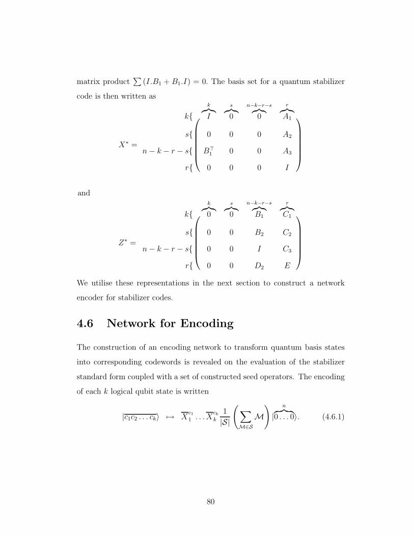
matrix product∑
(I.B1 + B1.I) = 0. The basis set for a quantum stabilizer
code is then written as
X∗ =
k{k︷︸︸︷I
s︷︸︸︷0
n−k−r−s︷︸︸︷0
r︷︸︸︷A1
s{ 0 0 0 A2
n− k − r − s{ B>1 0 0 A3
r{ 0 0 0 I
and
Z∗ =
k{k︷︸︸︷0
s︷︸︸︷0
n−k−r−s︷︸︸︷B1
r︷︸︸︷C1
s{ 0 0 B2 C2
n− k − r − s{ 0 0 I C3
r{ 0 0 D2 E
We utilise these representations in the next section to construct a network
encoder for stabilizer codes.
4.6 Network for Encoding
The construction of an encoding network to transform quantum basis states
into corresponding codewords is revealed on the evaluation of the stabilizer
standard form coupled with a set of constructed seed operators. The encoding
of each k logical qubit state is written
|c1c2 . . . ck〉 7→ Xc11 . . .X
ck
k
1
|S|
(∑
M∈S
M)|
n︷ ︸︸ ︷0 . . . 0〉. (4.6.1)
80

Let us consider the 8, 3, 5 qubit code [12, 31] with a stabilizer description
given by
M1 = X ⊗X ⊗X ⊗X ⊗X ⊗X ⊗X ⊗X
M2 = Z ⊗ Z ⊗ Z ⊗ Z ⊗ Z ⊗ Z ⊗ Z ⊗ Z
M3 = X ⊗ I ⊗X ⊗ I ⊗ Z ⊗ Y ⊗ Y ⊗ Y
M4 = X ⊗ I ⊗ Y ⊗ Z ⊗X ⊗ I ⊗ Y ⊗ Z
M5 = X ⊗ Z ⊗ I ⊗ Y ⊗ I ⊗ Y ⊗X ⊗ Z. (4.6.2)
The standard form associated with this set of operators and the seed operators
is derived as
X∗M =
1 0 0 0 1 1 1 00 1 0 0 1 1 0 10 0 1 0 1 0 1 11 1 1 0 0 1 1 10 0 0 0 1 0 0 00 0 0 0 0 1 0 00 0 0 0 0 0 1 00 0 0 0 0 0 0 1
Z∗M =
0 0 0 1 0 0 0 00 0 0 1 0 1 0 10 0 0 1 1 0 1 00 0 0 1 1 1 0 00 0 0 1 1 1 1 10 0 0 1 1 0 0 10 0 0 1 0 1 1 00 0 0 1 0 0 1 1
.
To encode this formalism, let us first consider a simplified version of the stan-
dard form in which we set Z∗M to vanish, and thus ignoring all phase shifts on
the code. Consequently, the matrix array X∗M is then given by the network in
Figure 4.1. While the encoding network implements bit-flip operations that
correspond to non-zero entries of X∗M , it also illustrates the importance of how
the standard form contributes to a clear exposition and an efficient computa-
tion. Let us now consider the action of phase shifts as seen by the matrix array
Z∗M on the encoding process. The action of a phase flip on a quantum states
serves only to alter the phase of that particular state. Since the phase flip does
not flip the individual state of the system, it follows that we can insert the set
of phase flips which corresponding to those non-zero elements of Z∗M into our
81

h
t
ht
ht
thhh
thhh
t
hhh
t
hhh
a4
a3
a2
a1
0
c3
c2
c1
Figure 4.1: Encoding network for X∗M .
encoding network where Y = X · Z. Finally, a complete network encoding is
achieved by implementing a Hadamard transform, H, on the last n− k qubits
with R = H · Z. A Hadamard transform of the last n − k qubits ensures
that the input states on the first k qudits, |c1c2c3〉, only determined the set of
codewords. Were this not the case then the last n − k inputs to the encoder
would influence the construction of the codewords since each of the last n− k
qubits in the state |0〉 would be flipped to the state |1〉. This would mean that
those qubits now flipped to |1〉 would help describe the codewords. Figure 4.2
illustrates the encoding circuit up to X∗MZ
∗M . The complete encoding circuit
is given in Figure 4.3.
82

Z Z
Z Z
Z Z
Z Z Z Z
Z Y
Y Y
Y Y
h
t
ht
ht
t
hh
t
h
t
h
h
t
hh
0
0
0
0
0
c3
c2
c1
Figure 4.2: Encoding network for X∗MZ
∗M .
R Z
R Z
H Z Z
R Z Z Z
Z Y
Y Y
Y Y
h
t
ht
ht
t
hh
t
h
t
h
h
t
hh
0
0
0
0
0
input
codeword
Figure 4.3: An Encoding Network for the [[8, 3, 5]] qubit code.
83
Chapter 5
Quantum Computation
5.1 Introduction
Introduced in his seminal paper, David Deutsch [24] proposed a new theory of
computation; the quantum theory of computation. Deutsch’s proposal copper-
fastened arguments given by Richard Feynman [29] that promised algorithms
to render many intractable classical problems feasible. By defining a computa-
tion predicated on exploiting inherently quantum phenomena, Deutsch offered
insights into the nature of quantum mechanics and provided a basis for the re-
alisation of a quantum computer. To realise a quantum computer one must be
concerned with the search for and implementation of quantum algorithms. A
quantum algorithm actuates quantum effects to perform computational tasks
with exponential speedup over its respective classical counterparts. Increased
theoretical and experimental research in the area of quantum computing is
providing such a basis for the discovery of further insights into the nature
of quantum algorithms. However, incidents of truely remarkable quantum
computing insights such as Shor’s factorisation algorithm are few in number.
Shor’s quantum algorithm was the first example of the exponential speedup in
resources over classical counterparts and that more examples of such insights
84

largely remain outside the confines of present knowledge stands in testament
to the understanding required to develop and exploit the theory of quantum
computing.
A quantum computer is in essence the realisation of quantum algorithms
which in many aspects is analogous to a classical computer with qudits re-
placing the classical bits as the conduit of information and unitary quantum
logic gates in respect of Boolean logic gates acting as operational elements. A
quantum logic gate is a transformation operator which is applied to a qudit
state in an equivalent fashion as a classical gate would be applied to a classical
bit. Furthermore, and in contrast to the classical case, quantum logic gates
must ensure that the superposition state of a qudit be maintained. This fea-
ture of quantum logic gates implies that the normalisation condition for qudit
states be preserved after the application of the operator.
The requirement of normalisation of transformed qudit states necessitates
the further precondition of unitarity on quantum logic gates. Unitarity is key
to setting the quantum and classical realms apart since transformed quantum
states must maintain coherence, or isolation from the environment. By the
linearity of quantum mechanics, it was shown (2.2.2) that unitarity of quan-
tum operators can only be preserved within a quantum system if the state
space of a qudit is isolated from the environment. Moreover, for the reason
that quantum logic gates are necessarily unitary transformations, quantum
gates are therefore said to exhibit a reversible nature. Herein lies a distin-
guishing feature of quantum computation since the reversible logic elements
exhibited in models of quantum computing do not lead to the irretrievable loss
of information associated with classical irreversible logic.
Since the theory of quantum computation is the theory of computation
then all classical irreversible operations must be resolved within the quantum
85

mechanical setting. To motivate an explanation for the nature of the exponen-
tial speedup in algorithm operation offered by quantum algorithms, we first
ought to consider at the picture of classical irreversibility. A reversible compu-
tation evaluates invertible functions f : {0, 1}n → {0, 1}n. Quantum circuitry
is fundamentally predisposed to this type of reversible computation since any
such computation can be reversed ensuring the existence of a suitable unitary
matrix for which f represents a legitimate quantum gate. In contrast, should
one consider the irreversible function f : {0, 1}n → {0, 1}m, n > m. Asso-
ciated with f is a gate with an m-bit range and n-bit domain. Each of the
m outputs can be characterised by one of the 22ndescriptions for a binary
function f : {0, 1}n 7→ {0, 1}. Therefore, there are (22n)mn×m gates that de-
scribe f of which only 2n! are reversible. The function f typifies many classical
irreversible gates such as AND, XOR, and NAND. Bennett [6] has shown that
any classical computation can be made reversible and therefore does not lead
to loss of entropy. Consider the function f given by f : {0, 1}n+m → {0, 1}n+m
where f (x; 0(m)) = (x; f(x)) and 0(m) denotes the setting of m-bits to zero.
Since f takes the inputs (x; 0(m)) to a distinct output then f can be extended
to an invertible function on n + m bits. Thus, for any irreversible function
f : {0, 1}n → {0, 1}m there is an invertible f which evaluates f . Understand-
ing how classical irreversibility can be made reversible in a quantum setting
may explain the delicate balance between loss of coherence, decoherence, in
the system and controlled computation of quantum algorithms.
1The set of functions f that describe arbitrary classical operations is as-
sociated with a corresponding set of logic gates. Furthermore, a set of gates
is called universal if instances of it are the only components required to repli-
cate the actions of all logic gates [26]. The quantum mechanical analogue
of the classical universal set of logic gates is a set of unitary operators that
86

generate the action of all unitary transformations in the Hilbert space. It was
shown that the 2-qubit controlled-NOT gate and the single rotational qubit
gate describes a universal set for quantum computation [3, 26]. Unitary trans-
formations act on quantum states and effect particular changes over a period
of time. A quantum state is therefore said to evolve under such transforma-
tions and correspondingly a time evolution operator acting on a quantum state
can always given by a unitary transformation. Suppose some quantum state
is given by |ψ〉 and further suppose there exists some unitary transformation
U acting on the state. If the state of the system is |ψ(t0)〉 at some initial
time t0 then its relation to the evolved state |ψ(t1)〉 at time t1 is given by
|ψ(t1)〉 = U(t1) |ψ(t0)〉 . Since U is an arbitrary operator, it is dependent on
the system and not on the initial state |ψ(t0)〉. The dynamics of U are de-
scribed by the action of some Hamiltonian H in Schrodinger’s equation [64].
To determine the dynamics of U , let us first consider a small increment in time
on |ψ(t)〉 under U . Hence, we have |ψ(t+4t)〉 = U(t +4t) |ψ(t)〉. Taking
a Taylor series expansion of U(t+4t) and coupled with the assumption of
H, it follows that U(t+4t) = 1 − ι/~H4t where ι2 = −1. The action of
U(t +4t) on the state |ψ(t)〉 is written |ψ(t+4t)〉 = (1 − ι/~H4t) |ψ(t)〉.
Hence,
|ψ(t+4t)〉 − |ψ(t)〉4t = − ι
~H |ψ(t)〉 , (5.1.1)
whence,
ι~∂ |ψ(t)〉∂t
= H |ψ(t)〉 . (5.1.2)
To determine the nature of the unitary transformation describing the time
evolved state |ψ(t1)〉, we consider the solution proposed by the Schrodinger
equation (5.1.2). Since H is a fixed Hermitian operator, we can deduce its
87

spectral decomposition. In particular, H has an orthonormal set of eigenvec-
tors |i〉 corresponding with real eigenvalues λi such that H |i〉 = λi |i〉. For
an arbitrary state |ψ(t)〉 =∑d−1
i=0 αi(t) |i〉, the time evolution of this arbitrary
state is described by the Schrodinger equation
ι~∂(∑d−1
i=0 αi(t) |i〉)∂t
= Hd−1∑
i=0
αi(t) |i〉
=d−1∑
i=0
αi(t)λi |i〉 (5.1.3)
and has solution
d−1∑
i=0
αi(t) |i〉 =d−1∑
i=0
e−ι/ λit1αi(t0) |i〉 (5.1.4)
Hence, for a time evolved state, t = t1, we have
|ψ(t1)〉 =
d−1∑
i=0
e−ι/ λit1αi(t0) |i〉
=
e−i/hλ0t1 0 . . . 0
0. . .
. . ....
.... . . 0
0 . . . 0 e−ι/ λd−1t1
d−1∑
i=0
αi(t0) |i〉
= U(t1) |ψ(t0)〉 . (5.1.5)
The matrix U(t1) = e−ι/ Ht1 maintains that the Hamiltonian H is a generator
of the unitary transformation U(t1). This is because the quantum mechanical
Hamiltonian operater H in the description of U(t1) corresponds to the total
energy of the system. From classical mechanics it follows that the energy
of the Hamiltonian operator generates the time evolution. Thus, any time
evolution on a quantum state in the Hilbert space is the result of applying the
Hamiltonian of the unitary transformation.
88

tj
|0〉 + |1〉
|0〉
|00〉 + |11〉
Figure 5.1: Controlled-NOT produces entangled states.
5.2 Multiple Quantum Gates
A universal quantum computer is a well-defined set of unitary gates that can
be designed to order the computation of quantum algorithms. Of crucial
importance for the successful performance of computations is this well-defined
set of gates. Thus far, we have considered the action of single quantum gates on
states. This description alone represents an incomplete model of computation.
The crux of successful quantum computation is the implementation of multiple
quantum gates. The most elementary of multiple quantum gates is to consider
some unitary operator U within a controlled-U two qubit operation. The
corresponding transformation given by transformation is written as |0〉 〈0| ⊗
I + |1〉 〈1| ⊗ U where the I operation represents the identity transformation.
This controlled two qubit operator is so called since the application of U on the
second qubit is decided by the state of the first qubit. The classic controlled-U
gate is the controlled-NOT gate. The action of a controlled-NOT gate with
respect to the computational basis is given as |x〉 |y〉 7→ |x〉 |y ⊕ x〉 where ⊕
represents addition modulo 2.
The controlled-NOT gate plays an important role in quantum computation
[27]. It is the quantum mechanical analogue of the classical connective XOR
gate and is a principle component for universal computations. It can be used
to produce maximally entangled states similar to the set of EPR pairs [60].
89

Furthermore, the controlled-NOT gate acts as a measurement gate [25] and
provides a basis for a so-called nondemolition measurement [22] that permits
the constuction of a syndrome table as used in error detection and correction.
5.3 Quantum Circuits
The quantum network approach to computation resembles the classical proce-
dure to computing [92] where quantum circuits are formed from a composition
of quantum states, quantum gates and quantum wires [61]. Computations are
described within the Hilbert spaceH = (Cd)⊗n
of n qudits where each horizon-
tal quantum wire corresponds to the individual Cd subspaces. Fundamental
to computation is the ability to store and control quantum information and
thus necessitates a suitable state space description to represent the information
vector. Computations are then a finite sequence of time-evolution quantum
gates set along the quantum wires to effect suitable transformations. Vertical
wires in a quantum circuit represent the coupling of arbitrary pairs of quan-
tum gates in a manner similar to a controlled-U gate. The depth of a circuit
refers to the maximum number of time evolution operators required to effect
necessary state changes. The width of a circuit is the maximum number of
gates in operation in any one time frame, and the complexity associated with
implementing a quantum circuit relates to the number of the gates needed
to solve the task. The task of constructing quantum circuitry architectures
is largely the problem of developing algorithms to describe various quantum
processes. Many theoretical approaches to quantum code design can now be
illustrated within a physical network. Computation of some inherently quan-
tum phenomenon by a quantum computer rests with the ability to find the
Hamiltonian for the Schrodinger equation which describes the dynamics of the
90

ht
th
ht|ψ〉
|φ〉
|φ〉
|ψ〉
Figure 5.2: Quantum circuit swapping two qubits.
phenomenon. This challenge degenerates to providing solutions to an expo-
nential number of differential equations that describe the Hamiltonian. The
growth of computations required for modest increases in the number of qudits
describing some quantum operation makes the classical computation of the
quantum system infeasible.
The crux of design and construction of a quantum computer operating in
a dn-dimensional Hilbert space lies with the suitable specification of quan-
tum gates that encode the support of a quantum code or implement quantum
algorithms. To realise such applications on a quantum computer requires cor-
responding gate circuitries that manipulate quantum states on both individual
and on controlled qudits. The controlled-NOT gate on a pair of qubits has
been experimentally realised by a string of ions in a linear Pauli trap [11].
The SWAP gate is an integral feature of the circuitry design of the quan-
tum Fourier transform. Figure 5.2 illustrates a quantum circuit swapping two
qubit by the repeated use of quantum controlled-NOT operators. Thus, the
question of designing a generalised quantum SWAP gate to implement a per-
mutation of quantum qudit states that utilize the generalised controlled-NOT
gate is a concern of universality in quantum computation in higher dimensional
quantum systems. How such designs can be extended within a mathematical
framework beyond the binary setting is of interest.
The concern of computation is to process information through the use a
well defined model that can be both understood algorithmically and realised
91

by some network topology. This is a concern encountered in both the classical
and quantum forms of computation where it is desirable that classes of com-
putation be implemented efficiently thereby requiring polynomial resources to
complete a task. While Shannon [74] demonstrated that most Boolean func-
tions require network topologies of exponential resources to compute, it was
Shor’s factorisation algorithm [79] that introduced the first model of quan-
tum computation to successfully exploit the laws of quantum mechanics and
process information efficiently. Such a model of computation now offered cre-
dence to years of speculative potential in the area by explicitly illustrating a
form that provided an exponential speedup in resources over the best known
classical form. It also signalled a marked increase in research into the means
of encoding classical information within quantum mechanical systems thereby
revealing aspects of what we now call a quantum computer.
Most often it is assumed that a quantum computer is predicated on a
collection of two-level quantum mechanical systems called qubits. However,
there has been the view to generalise to d-level, or qudit, quantum mechanical
systems. Implementing a quantum computer within a qubit or qudit frame-
work requires the ability to prepare a quantum state in a chosen basis, most
often maintained to be the computational basis, to perform a desired oper-
ation on some input state, and finally, to read the outcome of an operation
on an input state. While our knowledge of classical computation has influ-
enced the approach we take to implementing quantum computations, the task
of successfully implementing a quantum operation is made extremely difficult
by the phenomena of quantum parallelism and quantum entanglement. For-
tunately, the simultaneous interactions of quantum states expressed during
computation can be controlled to a degree by considering quantum opera-
tions as a composition of simpler operations on fewer quantum states. These
92

constituent operations are called quantum gates and surprisingly the only re-
striction quantum mechanics places on these gates is that they be unitary.
The influence classical computation renders on quantum computation is
again evident by mode of algorithm execution. The quantum circuit model
[24, 25] reflects the classical circuit and executes quantum algorithms by apply-
ing a sequence of quantum gates incrementally to act on one or more quantum
states. Those gates that have been experimentally demonstrated are said to
be elements of the quantum gate library. Unfortunately, there are only a
handful of quantum gates that can be experimentally realised within the co-
herence time of their systems [90]. However, Barenco et al. [3] showed that
any quantum operation on a set of n-qubits can be restricted to a composi-
tion of Controlled-NOT, CNOT, and single qubit gates. For this reason, we
say that the qubit gate library consisting of single qubit gates and CNOT is
universal. Furthermore, it has become standard in quantum information to
express any n-qubit quantum operation as a composition of single qubit gates
and CNOT gates. Consequently, the CNOT gate has acquired special status
as the hallmark of multiqubit control [91].
It is becoming increasingly evident that much effort continues to be made
into finding efficient quantum circuits in the sense that for the given gate
library there is no smaller circuit that achieves the same task. A reason for
this concerted effort is primarily due to the principle of decoherence. While
a quantum computer is predicated on the undisturbed evolution of quantum
coherences, decoherence represents a major but unavoidable problem for the
practical realization of quantum computers as it describes the error state of a
quantum computer which is introduced through the interaction of system and
environment. As with classical computation, the properties of experimentally
realisable quantum gates influence the execution time of quantum algorithms.
93

Since decoherence is unavoidable, it is therefore advantageous to ensure a
minimal use of computational resources to limit excution time and exposure
to the quantum environment. Thus, a minimal use of computational resources
serves to cap the total decohering time delivered by the execution of quantum
gates.
While universality is a key concern, the minimisation of gate counts is a
recent concern. To this end, research groups now focus on searching for uni-
versal n-qubit gates that contain fewest uses of CNOT gates [7, 8, 76, 77]. This
is because the cost of experimentally realising a CNOT gate exceeds the cost
associated by single qubit gates [8]. Consequently, construction of quantum
circuits that minimise the use of CNOT are important from the point of view
of execution time of the corresponding quantum algorithm which is positively
correlated with the decohering time of the circuit. Indeed, the experimental
realisation of a CNOT gate is a covented goal among quantum information
groups [91]. Experimental difficulties in realising certain quantum gates has
meant that universality of general n-qubit operations is a key motivation of
many quantum information groups. This is because both CNOT and single
qubit gates operations have now been experimentally realised. Universal quan-
tum circuits for an arbitrary two-qubit operator with six, four and three CNOT
gates have been found [78, 90, 91]. In fact, characterising the exact CNOT com-
plexity of an arbitrary n-qubit operation and constructing the corresponding
efficient quantum circuit is seen as an ambitious task, even by numerial anal-
ysis [91]. Research into universal circuit constructions have done considerable
work optimising their constructions [59]. In particular, Vatan and Williams
construct a quantum circuit for a general two-qubit operation that requires at
most three CNOT gates and fifteen one-qubit gates and show that their con-
struction is optimal [90]. However, crucial to this result is the demand that
94

quantum circuit for the two-qubit SWAP gate require at least three CNOT
gates [90]. To show the correctness of this claim, Vatan and Williams utilize
the notion of entangling power as introduced by Zanardi et. al [97]. More
recently, a scheme to realise the quantum SWAP gate between flying and sta-
tionary qubits has been presented by Liang and Li [53]. It is maintained [53]
that experimentally realising the quantum SWAP gate is a necessary condition
for the networkability of quantum computation. In fact, the SWAP gate can be
used to store quantum information, to teleport atomic or ionic states [53] and
is a fundamental element in the circuit implementation of Shor’s algorithm
[30].
Although universal two-qubit circuits with fewest uses of CNOT gates are
known, the three-qubit Toffoli gate is known to require at most six CNOT gates
[63], however, only five CNOT gates have been shown to be necessary [91]; see
also the references therein. More generally, devising quantum gate construc-
tions that extend to n-qubits remains an open problem. It is believed that
the study of quantum circuit minimisation and generalisation of qubit circuit
architectures to qudit circuit architectures will require different construction
techniques than those presently known. A geometric approach to quantum
circuit minimalisation has been put forward by Nielsen [59] that seeks to find
the length of a minimal geodesic with respect to a suitable Finsler metric. A
striking feature of this approach is that once an initial position and velocity of
the geodesic are determined the remainder of the geodesic can be completely
evaluated by a second order differential equation. This is in contrast with the
usual case of classical and quantum circuitry design where part of a circuit
does not aid the complete design. However, it is acknowledged the two-qubit
circuit synthesis can be used in a peephole optimization of larger circuits [78].
95

The problem of constructing an efficient quantum circuit for a given n-
qubit operation is seen as an important task for the complete networkability
of quantum computation. Unfortunately, the efficiency of universal designs
that accomplish this task is often known for the worst case of n-qubit opera-
tors. For example, the asymptotic number of CNOT gates used by Barenco’s
decomposition to implement any n-qubit operation is O(n34n) [76]. On the
other hand, it is believed that there are interesting operations which might
require a polynomial number of CNOT gates and that such operations might
also have an efficient construction within higher dimensional quantum sys-
tems. Indeed, considering new and efficient circuit designs within the qudit
setting taken with new approaches to circuitry design ought to be merit in
itself. However, in the context of information processing, it is maintained
that there are advantages in moving from the qubit paradigm to the qudit
paradigm. For instance, since the entropy of a message depends on the alpha-
bet used, it ought to be that and increasing the alphabet size should allow for
the construction of better error-correcting codes [36]. It has also been pointed
out that a quantum system composed of a pair of three dimensional subsystem
shows new features when compared to a two qubit system [36].
For efficient quantum computations, it is important to determine exactly
how many uses of the CNOT gate are required to effectuate a particular oper-
ation. We have seen that the optimal universal two-qubit circuit proposed by
Vatan and Williams [90] necessarily requires that the two-qubit SWAP gate
demands three CNOT gates. The SWAP gate has been illustrated to be a cor-
nerstone in the networkability of quantum computation. Therefore, a question
remains, can a generalised SWAP gate for higher dimensional quantum system
be efficiently constructed from generalised CNOT gates? Should this be the
case then the generalised SWAP gate for higher dimensional quantum systems
96

might be a cornerstone in the networkability of quantum computer based on
qudits. To this end, we note the following results.
5.4 On Permutations
Consider the set N = {1, 2, . . . , n} and let σ : N 7→ N be a bijection. We
say σ =
[1 2 . . . ni1 i2 . . . in
], where ik ∈ N is the image of k ∈ N under σ, is a
permutation of the set N.
Let σ and τ be two permutations of N. We define the product σ · τ by
(σ ·τ )(i) = σ(τ (i)), for i ∈ N, to be the composition of the mapping τ followed
by σ. These permutations taken with (·) form a group denoted Sn which is
called the symmetric group of degree n.
Given the permutation σ and for each i ∈ N, let us consider the sequence
i, σ(i), σ2(i), . . . . Since σ is a bijection and N is finite there exist a smallest
positive integer ` = `(i) depending on i such that σ`(i) = i. The orbit of i
under σ then consists of the elements i, σ(i), . . . , σ`−1(i). By a cycle of σ, we
mean the ordered set (i, σ(i), . . . , σ`−1(i)) which sends i into σ(i), σ(i) into
σ2(i),. . . , σ`−2(i) into σ`−1(i), and σ`−1(i) into i and leaves all other elements
of N fixed. Such a cycle is called an (`)-cycle. We refer to 2-cycles as trans-
positions. A pair of elements {σ(i), σ(j)} is an inversion in a permutation
σ if i < j and σ(i) > σ(j). Any permutation can be written as a product
of transpositions. The number of transpositions in any such product is even
if and only if the number of inversions is even, and consequently, we say the
permutation is even. Similarly, a permutation is odd if it can be written as a
product of an odd number of transposition and hence has an odd number of
inversions.
97
Lemma 1. Every permutation can be uniquely expressed as a product of dis-
joint cycles.
Proof: Let σ be a permutation. Then the cycles of the permutation are of
the form i, σ(i), . . . , σ`−1(i). Since the cycles are disjoint and by the multipli-
cation of cycles, we have it that the image of i ∈ N under σ is the same as
the image under the product, ς, of all the disjoint cycles of σ. Then, σ and ς
have the same effect on every element in N , hence, σ = ς.
Every permutation in Sn has then a cycle decomposition that is unique up
to ordering of the cycles and up to a cyclic permutation of the elements within
each cycle. Further, if σ ∈ Sn and σ is written as the product of disjoint cycles
of length n1, . . . , nk, with ni ≤ ni+1, we say (n1, . . . , nk) is the cycle type of σ.
As a result of Lemma 1, every permutation can be written as a product of
transpositions. Since the number of transpositions needed to represent a given
permutation is either even or odd, we define the signature of a permutation as
sgn(σ) =
{+1 if σ is even−1 if σ is odd
(5.4.1)
To each permutation, let us associate a permutation matrix Aσ whereby
Aσ(j, i) =
{1 if σ(i) = j0 otherwise
(5.4.2)
The mapping f : Sn 7→ det(Aσ) is a group homomorphism, where
det(Aσ) =∑
σ∈Sn
sgn(σ)
n∏
i=1
Aσ(i),i (5.4.3)
The kernel of this homomorphism, kerf , is the set of even permutations. Con-
sequently, we have it that σ is even if and only if det(Aσ) equals +1. The
kernel of the homomorphism signature defines the alternating group. Note
that the set of odd permutation can not form a subgroup but they form a
coset of the alternating group.
98
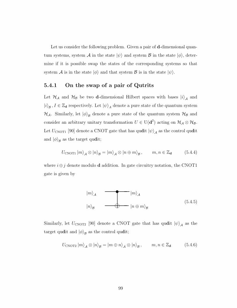
Let us consider the following problem. Given a pair of d-dimensional quan-
tum systems, system A in the state |ψ〉 and system B in the state |φ〉, deter-
mine if it is possible swap the states of the corresponding systems so that
system A is in the state |φ〉 and that system B is in the state |ψ〉.
5.4.1 On the swap of a pair of Qutrits
Let HA and HB be two d-dimensional Hilbert spaces with bases |i〉A and
|i〉B , I ∈ Zd respectively. Let |ψ〉A denote a pure state of the quantum system
HA. Similarly, let |φ〉B denote a pure state of the quantum system HB and
consider an arbitrary unitary transformation U ∈ U(d2) acting on HA ⊗HB.
Let UCNOT1 [90] denote a CNOT gate that has qudit |ψ〉A as the control qudit
and |φ〉B as the target qudit;
UCNOT1 |m〉A ⊗ |n〉B = |m〉A ⊗ |n⊕m〉B , m, n ∈ Zd (5.4.4)
where i⊕ j denote modulo d addition. In gate circuitry notation, the CNOT1
gate is given by
|m〉A
|n⊕m〉B|n〉B
|m〉Avj (5.4.5)
Similarly, let UCNOT2 [90] denote a CNOT gate that has qudit |ψ〉A as the
target qudit and |φ〉B as the control qudit;
UCNOT2 |m〉A ⊗ |n〉B = |m⊕ n〉A ⊗ |n〉B , m, n ∈ Zd (5.4.6)
99

vj =
1 0 0 0 0 0 0 0 00 1 0 0 0 0 0 0 00 0 1 0 0 0 0 0 00 0 0 0 1 0 0 0 00 0 0 0 0 1 0 0 00 0 0 1 0 0 0 0 00 0 0 0 0 0 0 0 10 0 0 0 0 0 1 0 00 0 0 0 0 0 0 1 0
vj
=
1 0 0 0 0 0 0 0 00 0 0 0 0 0 0 1 00 0 0 0 0 1 0 0 00 0 0 1 0 0 0 0 00 1 0 0 0 0 0 0 00 0 0 0 0 0 0 0 10 0 0 0 0 0 1 0 00 0 0 0 1 0 0 0 00 0 1 0 0 0 0 0 0
Figure 5.3: Matrix representations of CNOT types.
In gate circuitry notation, the CNOT2 gate is given by
|m⊕ n〉A
|n〉B|n〉B
|m〉Ajv (5.4.7)
Both circuits are read from left to right. Each horizontal line in both circuits
is called a wire and represents a finite dimensional quantum system. The
evolution of a quantum state over time is described by a set of unitary trans-
formations acting on the state description of the quantum system. Such state
evolutions are represented at various locations along the wire.
We now show that a swap of two qutrits is not possible using a composition
of CNOT gates alone. The point of this argument is to illustrate that a quan-
tum gate construction which permutes the states of three qutrit systems can
not be described by a set of qutrit transpositions induced by the CNOT gate
alone. Were this not the case then we would have a much simpler, with repect
to CNOT complexity, solution to the problem of construction a generalised
SWAP of d qudit system.
To show this, we first note that any sequence of CNOT gates acting on
the qutrit states |ψ〉A and |φ〉B can be written as a composition of the gates
100

CNOT1 and CNOT2. The CNOT1 and CNOT2 gates can be described in
the following way; the permutation matrix corresponding to the CNOT1 gate
takes the value 1 in row 3m + n and column 3m + (m ⊕ n), m, n = 0, 1, 2.
Similarly, the matrix corresponding to the CNOT2 gate takes the value 1 in
row 3m+ n column 3(m n) + n. These unitary matrix representations for a
CNOT gate are given in Fig. 5.3. Furthermore, both the CNOT1 matrix and
CNOT2 matrix have determinant +1 since the permutation corresponding to
each of the respective matrices is even.
Let us now assume that there exists a gate that swaps a pair of qutrit
states and that such a gate is composed using only the CNOT gate. Such a
swap gate will then be a composition of the gates CNOT1 and CNOT2. Since
each CNOT circuit acting on a pair of qutrits is a composition of CNOT1 and
CNOT2, it follows that any such composition will be equivalent to some prod-
uct of their respective unitary matrices. Such a product matrix product will
necessarily have determinant +1 as its constituent elements have determinant
+1. However, the matrix transformation representation required to effectuate
the swap of a pair of qutrits is given by
1 0 0 0 0 0 0 0 00 0 0 1 0 0 0 0 00 0 0 0 0 0 1 0 00 1 0 0 0 0 0 0 00 0 0 0 1 0 0 0 00 0 0 0 0 0 0 1 00 0 1 0 0 0 0 0 00 0 0 0 0 1 0 0 00 0 0 0 0 0 0 0 1
. (5.4.8)
This matrix takes the value 1 in row 3m+n column 3n+m and has determinant
-1. Thus, no composition of the former can yield the latter and the result
follows.
101

5.5 On the swap of a pair of qudits
Barenco et al. [3] showed that any unitary transformation on a set of qubits
can be decomposed into a sequence of CNOT and single-qubit gates [91]. We
now consider the problem of swapping a pair of d-dimensional quantum states
using only CNOT gates such that the system HA begins in the state |ψ〉A and
ends in the state |φ〉A while correspondingly the systemHB begins in the state
|φ〉B and ends in the state |ψ〉B. Our argument will be that a transposition
qudit states induces some unitary matrix U(d2) over HA ⊗HB whose circuit
architecture can not be completely determined by using only CNOT gates.
Recall the particular problem concerning the swap of a pair of qutrit sys-
tems. We have shown how the unitary matrices UCNOT1 and UCNOT2 both have
determinant +1. We also showed that this is in contrast to matrix USWAP
which describes the swapping of states of a pair of quantum systems where
such a matrix has determinant -1. Consequently, no compostion of CNOT
gates alone can induce the matrix that determines the action of the SWAP
gate. Another way to look at this is the following. The permutations
σCNOT1 =
(0 1 2 3 4 5 6 7 80 1 2 4 5 3 8 6 7
)
σSWAP =
(0 1 2 3 4 5 6 7 80 5 6 7 4 1 2 3 8
)(5.5.1)
that correspond to the unitary matrices UCNOT1 and USWAP have corresponding
cycle types (1, 1, 1, 3, 3) and (1, 1, 1, 2, 2, 2). Hence, a CNOT gate fixes three
basis states and permutes the remaining states in two cycles of length 3. Each
such cycle may be written as a product of two transpositions. Whence, the
signature of the CNOT permutation is +1. On the other hand, a SWAP
gate that swaps the states of a pairs of qutrits contains three fixed elements
and a set of three transpositions and therefore the signature of the SWAP
102
permutation is -1 and it follows that no composition of CNOT gates can lead
to an execution of a swap of a pair of qutrit systems.
More generally, a CNOT gate acting on a pair of d-dimensional quantum
systems corresponds to a permutation of the d2 basis states. We consider
the case when d = p is a prime. For prime dimensions d = p the case of
CNOT1, we have it that the basis states |m〉A ⊗ |n〉B of the system HAB
are mapped mapped to |m〉A ⊗ |n⊕m〉B. The permutation associated with
the CNOT1 mapping fixes d basis states and has (d − 1) cycles of length d,
each of which may be written as a product of d-1 transpositions. CNOT1
yields a permutation that can then be composed of (d− 1)2 transpositions of
qudit basis states. Similarly, the CNOT2 gate acting on a pair of qudit basis
states maps |m〉A ⊗ |n〉B of HAB to |m⊕ n〉A ⊗ |n〉B. There are d fixed basis
elements under the CNOT2 mapping and (d-1) cycles, each a product of d-1
transpositions. Therefore, the signature of the CNOT permutation is −1 for
dimension d = 2 and +1 for odd prime dimensions. Now suppose a CNOT
gate acting on a pair of qudits within system Hdd . Further suppose that such
an action is described by UCNOT ⊗ Idd−2. This matrix representation induces a
permutation of d(d−2) copies of the d2 basis elements targeted by the CNOT
gate and it follows that the signature of corresponding permutation is −1 only
for dimensions d = 2.
Let us consider a SWAP gate that swaps that states of a pair of qudits.
Such a gate corresponds to a permutation of the d2 basis states of system Hd2
which maps basis states |m〉A ⊗ |n〉B to basis states |n〉A ⊗ |m〉B. Under this
mapping there are d fixed basis elements and d(d−1)/2 transpositions which
describe the interchanging of all remaining basis states. Thus, the signature
of the permutation corresponding to the SWAP gate of a pair of qudits is −1
for dimensions d = 2 or 3 (mod 4) and +1 for dimensions d = 0 or 1 (mod
103

4). Thus when d = 3 (mod 4) the SWAP cannot be realised the CNOT gates
alone.
Further consider a cycle of d quantum states that maps basis states |u〉I ⊗
|v〉J ⊗ |w〉K · · · ⊗ |z〉M to the basis states |z〉I ⊗ |u〉J ⊗ |v〉K · · · ⊗ |y〉M. As
above the cycle structure of this permutation depends on the factorisation of
the dimension of the quantum system. Thus, for prime dimensions, the per-
mutation corresponding to a cycle of d qudit states contains d fixed states
and (dd−d)/d cycles of length d. Consequently, there are (d(d−1)−1)(d − 1)
transpositions association with the cycle of d qudit systems. Over even di-
mension d, the permutation signature of such is −1 and +1 for odd dimension
d.
The task swapping a pair of qudit states has been argued in terms of the
signature of a permutation. Based on this argument, we have shown that a
CNOT gate acting on a pair of qudits corresponds to a permutation whose
signature is +1, for odd prime dimensions. A SWAP of pairs of qudit systems
yields a permutation whose signature is −1 for dimensions d = 2 or 3 (mod
4) and +1 for dimensions d = 0 or 1 (mod 4). By this argument alone, circuit
architectures completely described by instances of the CNOT gate can not be
used to implement a SWAP of a pair of qudits for dimensions d = 3 (mod 4).
104

Chapter 6
On the WilNOT Gate
Of central importance to the theory of quantum computation is the role as-
sumed by single or multiple qudit gates that establish a basis for quantum cir-
cuitry designs. A quantum circuit is an assembly of discrete sets of components
which describe computational procedures [63]. A physical implementation of
such designs describes the process of computation whereby the evolution of a
qudit state and its influence on other states can be modelled. Quantum com-
putation is therefore a process that identifies the changes imposed on a quan-
tum state during the implementation of quantum gates in a manner analogous
to classical implementation of logic gates. Our ability to preserve quantum
coherence rests with our ability to implement efficient quantum computations.
Fundamental to successful quantum computations is the application of sin-
gle and multiple qudit gates. The most important multiple gate in the realm
of binary quantum computation is the two qubit controlled NOT gate [27]
as illustrated in Figure 5.1. The controlled NOT gate can realise quantum
computation networks such as entanglement, teleportation and error correc-
tion and is the principle multiple qubit gate in the universal set of gates that
describes arbitrary quantum computations [3, 63]. The dynamics of the con-
trolled NOT gate as described by its transformation on pairs of qubits can
105

be considered as an extension of the single gate NOT operation. In analogy
with the binary case, the generalised controlled NOT gate acts on two qudit
states. Correspondingly, the generalised NOT gate is crucial to the working
of the generalised controlled NOT gate and serves as the crux for popular
computations of error model and coding constructions in higher dimensions.
The qudit representation of a quantum state provides a natural mech-
anism by which quantum computations can be implemented. That such a
computation is made possible initially lies with the notion of state signature.
In particular, the correspondence of quantum information αk with a computa-
tional qudit basis element |k〉 and the subsequent genesis of the quantum state∑d−1
k=0 αk |k〉 in the Hilbert space Cd. Such a correspondence between informa-
tion and a Hilbert space representation is prerequisite to quantum computa-
tion since the successful transmission of any information state is predicated on
encoding the basis states associated with the quantum information elements
rather than the information itself which thereby prevents the collapse of the
state superposition and loss of information. This is in contrast to the classical
setting where no such correspondence is proffered nor required.
6.1 The WilNOT Gate
The WilNOT gate is a generalised quantum SWAP operator, see Figure 6.1.
By this I mean, suppose that the first quantum system A0 prepared in the
state |e0〉0, the second system A1 prepared in the state |e1〉1 and so forth, with
the final system Ad−1 prepared in the state |ed−1〉d−1. Construction of the
WilNOT gate over prime dimension yields a generalised SWAP gate so that
the system A0 is in the state |e1〉0, the system A1 is in the state |e2〉1 and
106

.
. . .
. . .
. . .
. . .
. . .
. . .
. . .
. . .
. . .
rf rf rf rf
. . .
. . .
. . .
. . .
. . .
. . .
. . .
. . .
. . .
......
......
. . .
. . .
. . .
. . .
. . .
. . .
. . .
. . .
. . .
f
rffff
fff
f
rffff
fff
f
rffff
fff
f
rffff
fff
rf r
f rf
. . . . . .
rf
rf
|e0〉0|e1〉1|e2〉2|e3〉3|e4〉4
|ed−1〉d−1
|ed−2〉d−2
|ed−4〉d−4
|ed−3〉d−3
.
. . .
. . .
. . .
. . .
. . .
. . .
. . .
. . .
. . .
......
...
r
f
r
f
r
f
r
f
......
......
r
f
r
f
r
frf rf rf f
r
. . .
. . .
. . .
. . .
. . .
. . .
. . .
. . .
. . .
. . .
. . .
. . .
. . .
. . .
. . .
. . .
. . .
. . . r
frf rf rf
. . .
. . .
. . .
. . .
. . .
. . .
. . .
. . .
. . .
rf
|e1〉0|e2〉1|e3〉2|e4〉3|e5〉4
|e0〉d−1
|ed−1〉d−2
|ed−3〉d−4
|ed−2〉d−3
Figu
re6.1:
The
WilN
OT
Gate;
AG
eneralised
SW
AP
Gate.
107
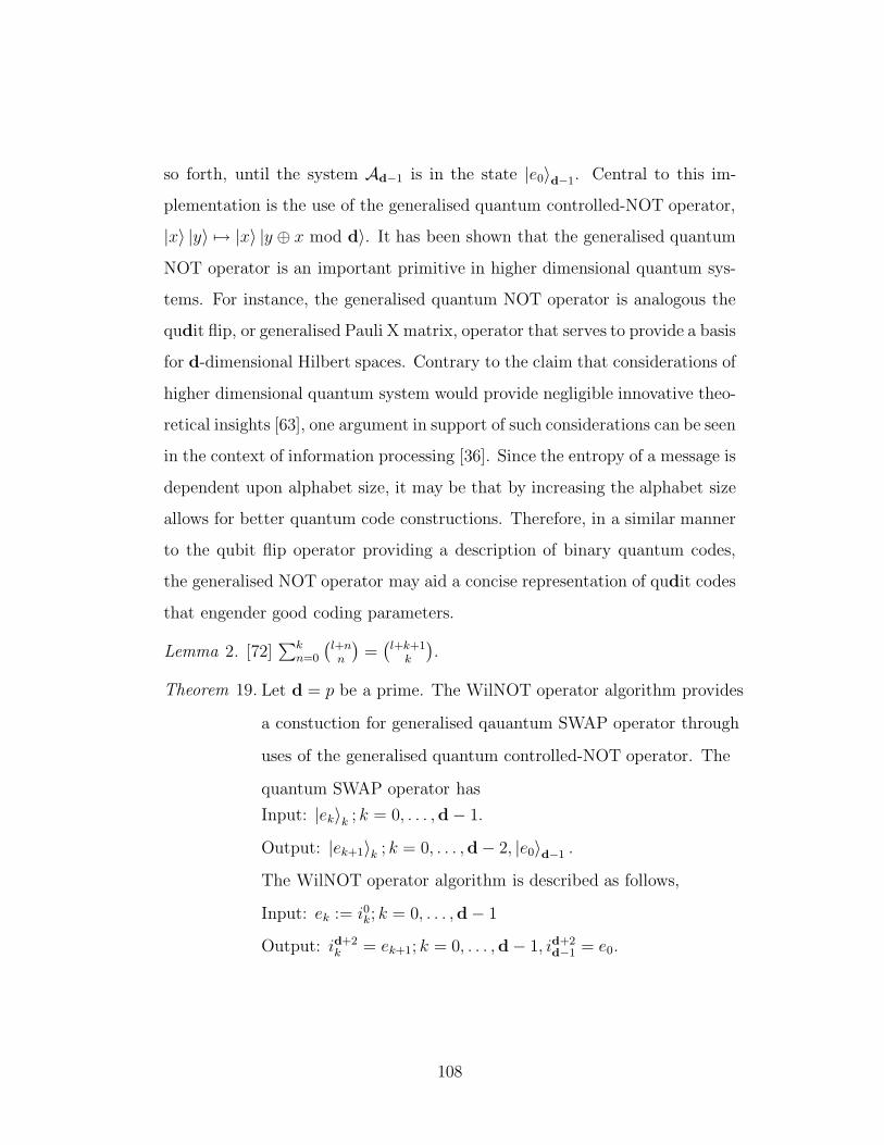
so forth, until the system Ad−1 is in the state |e0〉d−1. Central to this im-
plementation is the use of the generalised quantum controlled-NOT operator,
|x〉 |y〉 7→ |x〉 |y ⊕ x mod d〉. It has been shown that the generalised quantum
NOT operator is an important primitive in higher dimensional quantum sys-
tems. For instance, the generalised quantum NOT operator is analogous the
qudit flip, or generalised Pauli X matrix, operator that serves to provide a basis
for d-dimensional Hilbert spaces. Contrary to the claim that considerations of
higher dimensional quantum system would provide negligible innovative theo-
retical insights [63], one argument in support of such considerations can be seen
in the context of information processing [36]. Since the entropy of a message is
dependent upon alphabet size, it may be that by increasing the alphabet size
allows for better quantum code constructions. Therefore, in a similar manner
to the qubit flip operator providing a description of binary quantum codes,
the generalised NOT operator may aid a concise representation of qudit codes
that engender good coding parameters.
Lemma 2. [72]∑k
n=0
(l+nn
)=(
l+k+1k
).
Theorem 19. Let d = p be a prime. The WilNOT operator algorithm provides
a constuction for generalised qauantum SWAP operator through
uses of the generalised quantum controlled-NOT operator. The
quantum SWAP operator has
Input: |ek〉k ; k = 0, . . . ,d− 1.
Output: |ek+1〉k ; k = 0, . . . ,d− 2, |e0〉d−1 .
The WilNOT operator algorithm is described as follows,
Input: ek := i0k; k = 0, . . . ,d− 1
Output: id+2k = ek+1; k = 0, . . . ,d− 1, id+2
d−1 = e0.
108

Stage 1. Initialisation: j = 0.
ek := i0k
for k = 0, . . . ,d− 1.
The WilNOT gate is initiated by Stage 1 and step j = 0 by making the
correspondence between a representative input element i0k of the WilNOT
gate algorithm each standard basis state ek.
Stage 2. For j = 1, . . . ,d− 1.
ij0 = ij−10
ijk = ijk−1 + ij−1k ; k = 1, . . .d− 1.
Stage 2 consists of d − 1 steps which repeat the sequence of gates of
step j = 1. The sequence of gates at step j = 1, see Fig. 6.2, is tar-
geted on the systems A1, . . . ,Ad−1. Each step of Fig. 6.2 is a com-
position of CNOT gates acting on consecutive pairs of systems and
is written as a shorthand form to represent the sequence of CNOT
gates given in Fig. 6.3. The algorithm process of step j = 1 trans-
forms the input sequence i00, i01, i
02, . . . , i
0d−1 to the resulting state given
by i00,∑1
k=0 i0k,∑2
k=0 i0k, . . . ,
∑d−1k=0 i
0k. In a similar manner, the WilNOT
gate at step j = 2 takes the output from step j = 1 as input and repeats
the sequence of gates. The resulting state of the circuit at step j = 2
is given by i00, i00 +
∑1k=0 i
0k, i
00 +
∑1k=0 i
0k +
∑2k=0 i
0k, . . . , i
00 +
∑1k=0 i
0k +
∑2k=0 i
0k +· · ·+
∑d−1k=0 i
0k. This process continues to step j = d−1. Figure
6.4 illustrates initialisation on the circuit and the subsequent d−1 steps
of Stage 2.
109
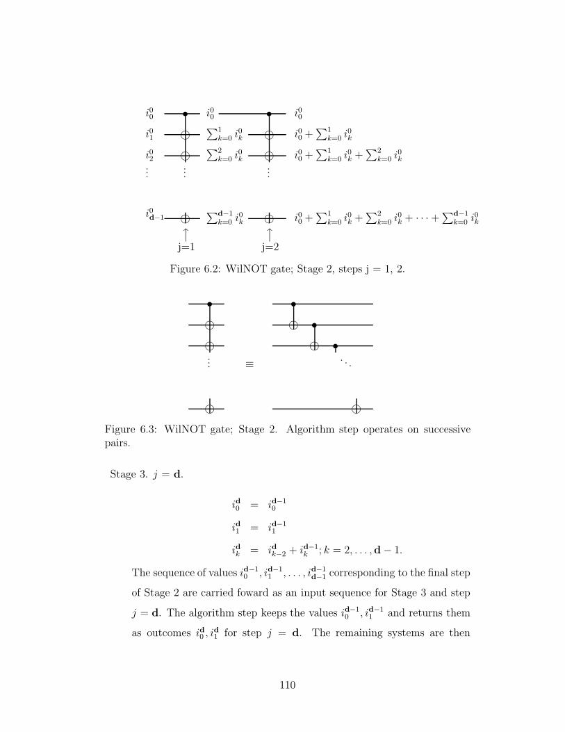
h hh
h
t th
i00∑1
k=0 i0k
∑2k=0 i
0k
∑d−1k=0 i
0k
i00
i00 +∑1
k=0 i0k
i00 +∑1
k=0 i0k +
∑2k=0 i
0k
i00 +∑1
k=0 i0k +
∑2k=0 i
0k + · · ·+
∑d−1k=0 i
0k
h
i01
i02
i00
......
...
i0d−1x x
j=1 j=2
Figure 6.2: WilNOT gate; Stage 2, steps j = 1, 2.
h hh
t tt
th
hh
.... . .≡
Figure 6.3: WilNOT gate; Stage 2. Algorithm step operates on successivepairs.
Stage 3. j = d.
id0 = id−10
id1 = id−11
idk = idk−2 + id−1k ; k = 2, . . . ,d− 1.
The sequence of values id−10 , id−1
1 , . . . , id−1d−1 corresponding to the final step
of Stage 2 are carried foward as an input sequence for Stage 3 and step
j = d. The algorithm step keeps the values id−10 , id−1
1 and returns them
as outcomes id0 , id1 for step j = d. The remaining systems are then
110

. . .
. . .
. . .
. . .
h hh
h
t tth h h
h
hh h
ht
i01
i02
i00
......
......
...
i0d−1
Figure 6.4: WilNOT gate; Stage 2, steps j = 1,. . . , d-1.
targeted in an iterative process. For instance, the outcome id2 for step
j = d is given by id0 + id−12 . This value is then stored as the result id2
for e2 at Stage 3. The outcome state for A0,A1,A2 at Stage 3 have thus
been determined. To evaluate the result value for A3, the algorithm
computes id1 + id−13 and stores this value as the outcome id3 for Stage 3.
Figure 6.5 illustrates the process that determines the current state of the
algorithm following stage 3 and step j = d in diagrammatic shorthand
form for the sequence of CNOTs.
Stage 4. j = d+1.
id+1k = idk + idk+1
id+1d−1 = idd−1; k = 0, . . . ,d− 2.
Stage 4 consists of a single step, j = d+1, whose primary algorithm oper-
ation acts as a CNOT on the d-1 consecutive pairs of systems (Ak,Ak+1)
for k = 0, . . . ,d − 2, computing (idk + idk+1) and storing these values as
the outcome id+1k . The value idd−1 is returned as the outcome id+1
d−1.
111
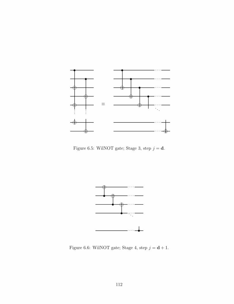
≡
h
hh
h
h
tt
......
. . .
. . .
. . .
. . .
. . .
. . .
. . .
. . .
hh
h
h
t
tt
t
Figure 6.5: WilNOT gate; Stage 3, step j = d.
. . .
. . .
. . .
. . .
. . .
. . .
hh
h
t
tt
t
Figure 6.6: WilNOT gate; Stage 4, step j = d + 1.
112

. . .
. . .
. . .
. . .
. . .
. . .
. . .
......
...
t
h
t
h
t
h
t
h
......
......
t
h
t
h
t
h h
t
. . .
. . .
. . .
. . .
. . .
. . .
. . .
. . .
. . .
. . .
. . .
. . .
. . .
. . .
. . . th
th
th
. . .
. . .
. . .
. . .
. . .
. . .
. . .
th
id+20
id+21
id+22
id+23
id+2d−1
id+2d−2.
id+2d−3
Figure 6.7: WilNOT gate; Stage 5, step j = d + 2.
Stage 5. j = d+2.
id+2k = id+1
k
id+2d−1 = id+1
d−1 +d−2∑
k=0
ηkid+2k ; k = 0, . . . ,d− 2
with
d−2∑
k=0
ηkid+2k :=
bd−22
c∑
t=0
(d − 1)id+22t+1 +
d−32∑
t=0
id+22t (6.1.1)
Stage 5 concludes the WilNOT gate transformation with a set of gates
targeted on system Ad−1 whose current state is represented by id+1d−1 . The
values id+20 , id+2
1 , . . . , id+2d−2 for the respective systems A0,A1, . . . ,Ad−2
are unchanged from their representative values id+10 , id+1
1 , . . . , id+1d−2 at step
j = d + 1 and are returned as outcomes in the final state for step j =
113

d+2. The final state of Ad−1 is given by id+2d−1 = id+1
d−1 +∑d−2
k=0 ηkid+2k
= id+1d−1 +id+1
0 +(d−1)id+11 +id+1
2 +(d−1)id+13 +· · ·+id+1
d−3 +(d−1)id+1d−2 .
Thus, for odd valued k there is a gate with id+2k as control and for even
valued k there are d-1 gates with id+2k as control. This is represented in
Figure 6.7.
Proof : We show that the algorithm outputs id+2k = ek+1 for k = 0, . . . ,d+2
and id+2d−1 = e0. At step j = 0, we have it that,
ek := i0k; k = 0, ...,d− 1.
At Stage 2, step j = 1 the algorithm sets i10 = i00 and computes i11 as
i11 = i10 + i01. Similarly, i12 = i11 + i02 = i00 + i01 + i02 =∑2
m=0 i0m. Therefore, for
k = 1, . . . ,d− 1, we have,
i1k = i1k−1 + i0k
= i1k−2 + i0k−1 + i0k
= i1k−3 + i0k−2 + i0k−1 + i0k
= . . .
= i10 + i01 + i02 + · · ·+ i0k−3 + i0k−2 + i0k−1 + i0k
=k∑
m=0
i0m (6.1.2)
The next step, Stage 2 step j = 2, implements a repeat set of gates of step
1. By definition i20 = i10 = i00. The case for k = 1, . . . ,d − 1 follows from the
algorithm step,
i2k = i2k−1 + i1k
= i2k−2 + i1k−1 + i1k
= . . .
114

= i20 + i11 + i12 + · · ·+ i1k−2 + i1k−1 + i1k
= i00 +1∑
m=0
i0m +2∑
m=0
i0m + · · ·+k∑
m=0
i0m
=
k∑
l=0
l∑
m=0
i0m
=k∑
m=0
k∑
l=m
i0m
=k∑
m=0
k−m∑
l=0
i0m
=
k∑
m=0
(k −m+ 1
1
)i0m (6.1.3)
We show by induction that, for j = 1, . . . ,d − 1, ijk =∑k
m=0
(k−m+j−1
j−1
)i0m,
k = 0, . . . ,d−1. We have shown that this is true for j = 1. Let 1 ≤ j < d−1
and suppose that
ijk =
k∑
m=0
(k −m+ j − 1
j − 1
)i0m, (6.1.4)
k = 0, . . . ,d− 1 Now, ij+10 = ij0 = i00. For 1 ≤ k ≤ d− 1, we have
ij+1k = ijk + ij+1
k−1
= ijk + ijk−1 + ij+1k−2
= . . .
= ijk + ijk−1 + · · ·+ ij2 + ij1 + ij+10
= ijk + ijk−1 + · · ·+ ij2 + ij1 + ij0. (6.1.5)
Since ij+10 = ij0 follows from the algorithm step, we have it that ij+1
k =∑k
m=0 ijm. Hence, by the induction process,
115

ij+1k =
k∑
m=0
ijm = i00 +1∑
l=0
(1− l + j − 1
j − 1
)i0l +
2∑
l=0
(2 − l + j − 1
j − 1
)i0l + . . .
+
k∑
l=0
(k − l+ j − 1
j − 1
)i0l
=k∑
m=0
m∑
l=0
(m− l+ j − 1
j − 1
)i0l
=k∑
m=0
k∑
l=0
(m− l+ j − 1
j − 1
)i0l
=
k∑
l=0
k∑
m=l
(m− l + j − 1
j − 1
)i0l
=k∑
l=0
(k − l + j
j
)i0l . (6.1.6)
Therefore, the result is true for j + 1
ij+1k =
k∑
m=0
(k −m+ j
j
)i0m (6.1.7)
and the result follows by induction.
The algorithm at Stage 3, step j = d
id0 = id−10 = i00
id1 = id−11 =
1∑
m=0
(1−m+ d− 2
d− 2
)i0m = (d− 1)i00 + i01. (6.1.8)
Implementing the algorithm step idk = idk−2 + id−1k for k = 2, . . . d − 1, we
have it that
id2 = id0 + id−12 = i00 +
2∑
m=0
(2 −m+ d − 2
d − 2
)i0m
116

id3 = id1 + id−12 =
1∑
m=0
(1−m+ d− 2
d− 2
)i0m +
3∑
m=0
(3 −m+ d− 2
d− 2
)i0m
id4 = id2 + id−14 = i00 +
2∑
m=0
(2 −m+ d − 2
d − 2
)i0m +
4∑
m=0
(4−m+ d− 2
d− 2
)i0m
. . .
Therefore for odd valued k,
idk =
k−12∑
t=0
2t+1∑
m=0
(2t+ 1−m+ d− 2
d− 2
)i0m
=
k−12∑
t=0
2t+1∑
m=2t
(2t+ 1−m+ d− 2
d− 2
)i0m (as d is prime)
=
k−12∑
t=0
(d − 1)i02t + i02t+1 (6.1.9)
and similarly for even valued k,
idk =
k2∑
t=0
2t∑
m=0
(2t−m+ d− 2
d− 2
)i0m
=
k2∑
t=0
2t∑
m=2t
(2t−m+ d − 2
d− 2
)i0m (as d is prime)
=
k2∑
t=0
(d− 1)i02t−1 + i02t. (6.1.10)
Stage 4, step j = d + 1 of the algorithm is given by id+1k = idk + idk+1 for
k = 0, . . . ,d− 2. Let us consider id+1k . There are two cases; for even valued k
we note that
idk = idk−2 + id−1k
117

= idk−4 + id−1k−2 + id−1
k
= . . .
=
k2∑
t=0
id−12t (6.1.11)
while
idk+1 = idk−1 + id−1k+1
= idk−3 + id−1k−1 + id−1
k+1
= . . .
=
b k+12
c∑
t=0
id−12t+1. (6.1.12)
Therefore, id+1k =
∑k+1t=0 i
d−1t . Alternatively, for odd valued k then idk =
∑ k−12
t=0 id−12t+1 while idk+1 =
∑ k+12
t=0 id−12t and id+1
k =∑k+1
t=0 id−1t . Hence,
id+1k =
k+1∑
t=0
id−1l
=k+1∑
l=0
t∑
m=0
(t−m+ d− 2
d− 2
)i0m
=
k+1∑
m=0
k+1∑
l=m
(l−m+ d− 2
d− 2
)i0m
=k+1∑
m=0
(k −m+ d
d− 1
)i0m
= i0k+1 mod d. (6.1.13)
Recall that since the dimesion, d = p, considered is prime, under arithmetic
modulo d,(k−m+d
d−1
)vanishes for m 6= k + 1 and therefore we deduce that
id+1k = i0k+1 for k = 0, . . . ,d− 2. When k = d-1 we have
id+1d−1 = idd−1 =
bd−12
c∑
t=0
2t∑
m=0
(2t−m+ d− 2
d − 2
)i0m. (6.1.14)
118
The WilNOT gate concludes at Stage 5 step j = d+2 with the implemen-
tation of a sequence of gates targeted on id+1d−1. For k = 0, . . . ,d − 2, we have
the result
id+2k = id+1
k = i0k+1 mod d. (6.1.15)
For k = d − 1, the value of id+2d−1 is given by
id+2d−1 = id+1
d−1 +d−2∑
k=0
ηkid+2k
=
bd−12
c∑
t=0
2t∑
m=0
(2t−m+ d− 2
d− 2
)i0m +
d−2∑
k=0
ηkid+2k .
To show that this returns the desired result, we consider the value id+1d−1 mod d.
Lemma 3. id+1d−1 mod d =
∑bd−12
ct=0 i02t +
∑bd−12
c−1
t=0 (d− 1)i02t+1.
Proof.
id+1d−1 =
d−12∑
t=0
2t∑
m=0
(2t−m+ d − 2
d− 2
)i0m
=
d−1∑
m=0
d−12∑
t=dm2e
(2t−m+ d− 2
d− 2
)i0m. (6.1.16)
Since(2t−m+d−2
d−2
)= 0 mod d for t > dm
2e then
id+1d−1 mod d =
d−1∑
m=0
(2dm
2e −m+ d − 2
d− 2
)i0m
=
d−12∑
l=0
i02l +
bd−22
c∑
l=0
(d− 1)i02l+1. (6.1.17)
Thus, id+1d−1 mod d =
∑d−12
t=0 i02t +
∑bd−22
ct=0 (d − 1)i02t+1. By definition of Stage 5,
we have it that∑d−2
k=0 ηkid+2k =
∑bd−22
ct=0 (d− 1)id+2
2t+1 +∑d−3
2t=0 i
d+22t . The value of
119
id+2d−1 is then given by
id+2d−1 = id+1
d−1 +d−2∑
k=0
ηkid+2k
=
bd−12
c∑
t=0
i02t +
bd−22
c∑
t=0
(d− 1)i02t+1 +
bd−22
c∑
t=0
i02t+1 +
bd−12
c∑
t=1
(d− 1)i02t. (6.1.18)
Consequently, id+2d−1 mod d = id+2
0 = i00. Stage 5 of the algorithm ensures that
the WilNOT gate effectuates the transformation of an input sequence given
by i0k = ek for k = 0, . . . ,d−1 to the sequence id+2k = ek+1 for k = 0, . . . ,d−2
and id+1d−1 = e0, thereby finalising the construction process for a generalised
quantum SWAP gate. We show that the network SWAPS all dd sequences of
input states.
Theorem 20. LetA0, . . . ,Ad−1 be d-dimensional systems with bases |e0〉j , |e1〉j,
. . . , |ed−1〉j , j = 0, . . . ,d−1, where e0, . . . , ed−1 ∈ Zd. LetA = A0⊗· · ·⊗Ad−1.
If a network implements a SWAP on each basis state |a0a1 . . . ad−1〉 = |a0〉0⊗
|a1〉1 ⊗ · · · ⊗ |ad−1〉d−1 of A where a0, . . . , ad−1 ∈ Zd then the network imple-
ments a SWAP on any input state |ψ〉 = |ψ0〉0 ⊗ |ψ1〉1 ⊗ |ψd−1〉d−1.
Proof: Let |ψj〉j =∑d−1
kj=0 αjkj
∣∣ekj
⟩j, j = 0, . . . ,d− 1. Then
|ψ〉 =d−1∑
k0=0
· · ·d−1∑
kd−1
α0k0 . . . α(d−1)kd−1|k0 . . . kd−1〉 . (6.1.19)
Now,
SWAP(|ψ〉) =d−1∑
k0=0
· · ·∑
kd−1
α0k0 . . . α(d−1)kd−1SWAP(|k0 . . . kd−1〉)
=d−1∑
k0=0
· · ·d−1∑
kd−1
α0k0 . . . α(d−1)kd−1|k1 . . . kd−1k0〉
=d−1∑
k1=0
· · ·d−1∑
kd−1
d−1∑
k0=0
α1k1 . . . α(d−1)kd−1α0k0 |k1 . . . kd−1k0〉
= |ψ1〉0 ⊗ · · · ⊗ |ψd−1〉d−2 ⊗ |ψ0〉d−1 (6.1.20)
120

hht t
hh
th
tt
hh
tt t
h h h
∑2i=0 ai |i〉
∑2i=0 bi|i〉
∑2i=0 ci|i〉
∑2i=0 ai |i〉
∑2i=0 bi|i〉
∑2i=0 ci|i〉
Figure 6.8: Qutrit WilNOT SWAP Network.
as required.
In particular, for an input quantum state of a d-fold quantum system
whose first system A0 is prepared in the state |e0〉0, whose second system
A1 is prepared in the state |e1〉1 and so forth, and whose final system Ad−1
of the input state is prepared in the state |ed−1〉d−1, an application of the
WilNOT gate over prime dimensions yields a generalised SWAP gate so that
the system A0 is in the state |e1〉0, the system A1 is in the state |e2〉1 and so
forth, until the system Ad−1 is in the state |e0〉d−1. Furthermore, a WilNOT(l),
l < d, operator composed of l repeating WilNOT gates can be constructed
to effectuate a cyclic shift of quantum states through l quantum systems of a
d-fold qudit system.
6.2 WilNOT Example: The Qutrit Case
The qubit network that swaps two arbitrary qubit states is well known [60].
When restricted to the qubit setting, the WilNOT operator yields the unitary
transformation matrices that swap the states of a pair of arbitrary qubits. We
give an example of how WilNOT is used to swap the information content of
three arbitrary qutrit states by defining the required unitary transformation
121

matrices, see Figure 6.8. For the case d=3 the WilNOT operator produces
the following sequence of states of systems A0,A1,A2 on input |i〉0 , |j〉1 , |k〉2.
Stage 1. |i〉0 |j〉1 |k〉2Stage 2, step 1. |i〉0 |i+ j〉1 |i+ j + k〉2Stage 2, step 2. |i〉0 |2i+ j〉1 (|3i+ 2j + k〉2 = |2j + k〉2)
Stage 3. |i〉0 |2i+ j〉1 |i+ 2j + k〉2Stage 4. (|3i+ j〉0 = |j〉0)(|3i+ 3j + k〉1 = |k〉1 |i+ 2j + k〉2Stage 5. |j〉0 |k〉1 (|i+ 3j + 3k〉2 = |i〉2)
The unitary transformation matrices associated with the WilNOT operator
over C27 ≡ C33are as follows; let U1 be the unitary transformation correspond-
ing to Stage 1, step 1. Then U1(|i〉0 |j〉1 |k〉2) = |i〉0 |i+ j〉1 |i+ j + k〉2. Let
|a〉0 =∑2
i=0 ai |i〉, |b〉1 =∑2
i=0 bi |i〉, |c〉2 =∑2
i=0 ci |i〉. Then we may write
|a〉0 ⊗ |b〉1 ⊗ |c〉2 as∑2
i1=0
∑2i2=0
∑2i3=0 ai1bi2ci3 |i1i2i3〉 . Thus
U1(|a〉0 ⊗ |b〉1 ⊗ |c〉2)
= U1 ((a0 |0〉 + a1 |1〉 + a2 |2〉)⊗ (b0 |0〉+ b1 |1〉 + b2 |2〉)⊗ (c0 |0〉 + c1 |1〉+ c2 |2〉))
= U1(a0b0c0 |000〉 + a0b0c1 |001〉 + a0b0c2 |002〉 + a0b1c0 |010〉 + a0b1c1 |011〉
+a0b1c2 |012〉 + a0b2c0 |020〉 + a0b2c1 |021〉 + a0b2c2 |022〉 + a1b0c0 |100〉
+a1b0c1 |101〉 + a1b0c2 |102〉 + a1b1c0 |110〉 + a1b1c1 |111〉 + a1b1c2 |112〉
+a1b2c0 |120〉 + a1b2c1 |121〉 + a1b2c2 |122〉 + a2b0c0 |200〉 + a2b0c1 |201〉
+a2b0c2 |202〉 + a2b1c0 |210〉 + a2b1c1 |211〉 + a2b1c2 |212〉 + a2b2c0 |220〉
+a2b2c1 |221〉 + a2b2c2 |222〉)
= a0b0c0 |000〉 + a0b0c1 |001〉 + a0b0c2 |002〉 + a0b1c0 |011〉 + a0b1c1 |012〉
+a0b1c2 |010〉 + a0b2c0 |022〉 + a0b2c1 |020〉 + a0b2c2 |021〉 + a1b0c0 |111〉
+a1b0c1 |112〉 + a1b0c2 |110〉 + a1b1c0 |122〉 + a1b1c1 |120〉 + a1b1c2 |121〉
+a1b2c0 |100〉 + a1b2c1 |101〉 + a1b2c2 |102〉 + a2b0c0 |222〉 + a2b0c1 |220〉
122

+a2b0c2 |221〉 + a2b1c0 |200〉 + a2b1c1 |201〉 + a2b1c2 |202〉 + a2b2c0 |211〉
+a2b2c1 |212〉 + a2b2c2 |210〉 . (6.2.1)
Thus for Stage 2, step 1 the matrix corresponding to U1 is (for the usual
lexicographic ordering for rows and coloumns)
U1 =
1 0 0 0 0 0 0 0 0 0 0 0 0 0 0 0 0 0 0 0 0 0 0 0 0 0 00 1 0 0 0 0 0 0 0 0 0 0 0 0 0 0 0 0 0 0 0 0 0 0 0 0 00 0 1 0 0 0 0 0 0 0 0 0 0 0 0 0 0 0 0 0 0 0 0 0 0 0 00 0 0 0 0 1 0 0 0 0 0 0 0 0 0 0 0 0 0 0 0 0 0 0 0 0 00 0 0 1 0 0 0 0 0 0 0 0 0 0 0 0 0 0 0 0 0 0 0 0 0 0 00 0 0 0 1 0 0 0 0 0 0 0 0 0 0 0 0 0 0 0 0 0 0 0 0 0 00 0 0 0 0 0 0 1 0 0 0 0 0 0 0 0 0 0 0 0 0 0 0 0 0 0 00 0 0 0 0 0 0 0 1 0 0 0 0 0 0 0 0 0 0 0 0 0 0 0 0 0 00 0 0 0 0 0 1 0 0 0 0 0 0 0 0 0 0 0 0 0 0 0 0 0 0 0 00 0 0 0 0 0 0 0 0 0 0 0 0 0 0 1 0 0 0 0 0 0 0 0 0 0 00 0 0 0 0 0 0 0 0 0 0 0 0 0 0 0 1 0 0 0 0 0 0 0 0 0 00 0 0 0 0 0 0 0 0 0 0 0 0 0 0 0 0 1 0 0 0 0 0 0 0 0 00 0 0 0 0 0 0 0 0 0 0 1 0 0 0 0 0 0 0 0 0 0 0 0 0 0 00 0 0 0 0 0 0 0 0 1 0 0 0 0 0 0 0 0 0 0 0 0 0 0 0 0 00 0 0 0 0 0 0 0 0 0 1 0 0 0 0 0 0 0 0 0 0 0 0 0 0 0 00 0 0 0 0 0 0 0 0 0 0 0 0 1 0 0 0 0 0 0 0 0 0 0 0 0 00 0 0 0 0 0 0 0 0 0 0 0 0 0 1 0 0 0 0 0 0 0 0 0 0 0 00 0 0 0 0 0 0 0 0 0 0 0 1 0 0 0 0 0 0 0 0 0 0 0 0 0 00 0 0 0 0 0 0 0 0 0 0 0 0 0 0 0 0 0 0 0 0 1 0 0 0 0 00 0 0 0 0 0 0 0 0 0 0 0 0 0 0 0 0 0 0 0 0 0 1 0 0 0 00 0 0 0 0 0 0 0 0 0 0 0 0 0 0 0 0 0 0 0 0 0 0 1 0 0 00 0 0 0 0 0 0 0 0 0 0 0 0 0 0 0 0 0 0 0 0 0 0 0 0 0 10 0 0 0 0 0 0 0 0 0 0 0 0 0 0 0 0 0 0 0 0 0 0 0 1 0 00 0 0 0 0 0 0 0 0 0 0 0 0 0 0 0 0 0 0 0 0 0 0 0 0 1 00 0 0 0 0 0 0 0 0 0 0 0 0 0 0 0 0 0 0 1 0 0 0 0 0 0 00 0 0 0 0 0 0 0 0 0 0 0 0 0 0 0 0 0 0 0 1 0 0 0 0 0 00 0 0 0 0 0 0 0 0 0 0 0 0 0 0 0 0 0 1 0 0 0 0 0 0 0 0
. (6.2.2)
(6.2.3)
The state returned after step 1, is now an entangled state. This is beacause
there is a positive entangling power measure associated with the CNOT gate
123

[90]. As we seek a generalised quantum SWAP gate, we have by extension of
the qubit SWAP gate, to construct a quantum gate whose entangling power
measure is zero [90]. The state of the WilNOT gate is remains entangled until
all the unitary transformations described by WilNOT are applied. The set of
unitary transformations are given by definition of each step in WilNOT. We
now give the remaining set of unitarity transformations and the action of each
unitary on the corresponding input states.
The unitary matrix corresponding to Stage 2, step 2 is the same as U1. Let
the transformation corresponding to Stage 2 of WilNOT be U2. So U2 = U21 .
We may write the action of U2 on the state of the system prior to application
of step 2 of WilNOT as
U2(|a〉 ⊗ |b〉 ⊗ |c〉)
= U1(a0b0c0 |000〉 + a0b0c1 |001〉 + a0b0c2 |002〉 + a0b1c0 |011〉 + a0b1c1 |012〉
+a0b1c2 |010〉 + a0b2c0 |022〉 + a0b2c1 |020〉 + a0b2c2 |021〉 + a1b0c0 |111〉
+a1b0c1 |112〉 + a1b0c2 |110〉 + a1b1c0 |122〉 + a1b1c1 |120〉 + a1b1c2 |121〉
+a1b2c0 |100〉 + a1b2c1 |101〉 + a1b2c2 |102〉 + a2b0c0 |222〉 + a2b0c1 |220〉
+a2b0c2 |221〉 + a2b1c0 |200〉 + a2b1c1 |201〉 + a2b1c2 |202〉 + a2b2c0 |211〉
+a2b2c1 |212〉 + a2b2c2 |210〉)
= a0b0c0 |000〉 + a0b0c1 |001〉 + a0b0c2 |002〉 + a0b1c0 |012〉 + a0b1c1 |010〉
+a0b1c2 |011〉 + a0b2c0 |021〉 + a0b2c1 |022〉 + a0b2c2 |020〉 + a1b0c0 |120〉
+a1b0c1 |121〉 + a1b0c2 |122〉 + a1b1c0 |102〉 + a1b1c1 |100〉 + a1b1c2 |101〉
+a1b2c0 |111〉 + a1b2c1 |112〉 + a1b2c2 |110〉 + a2b0c0 |210〉 + a2b0c1 |211〉
+a2b0c2 |212〉 + a2b1c0 |222〉 + a2b1c1 |220〉 + a2b1c2 |221〉 + a2b2c0 |201〉
+a2b2c1 |202〉 + a2b2c2 |200〉 . (6.2.4)
124

The matrix corresponding to U2 is
U2 =
1 0 0 0 0 0 0 0 0 0 0 0 0 0 0 0 0 0 0 0 0 0 0 0 0 0 00 1 0 0 0 0 0 0 0 0 0 0 0 0 0 0 0 0 0 0 0 0 0 0 0 0 00 0 1 0 0 0 0 0 0 0 0 0 0 0 0 0 0 0 0 0 0 0 0 0 0 0 00 0 0 0 0 1 0 0 0 0 0 0 0 0 0 0 0 0 0 0 0 0 0 0 0 0 00 0 0 1 0 0 0 0 0 0 0 0 0 0 0 0 0 0 0 0 0 0 0 0 0 0 00 0 0 0 1 0 0 0 0 0 0 0 0 0 0 0 0 0 0 0 0 0 0 0 0 0 00 0 0 0 0 0 0 1 0 0 0 0 0 0 0 0 0 0 0 0 0 0 0 0 0 0 00 0 0 0 0 0 0 0 1 0 0 0 0 0 0 0 0 0 0 0 0 0 0 0 0 0 00 0 0 0 0 0 1 0 0 0 0 0 0 0 0 0 0 0 0 0 0 0 0 0 0 0 00 0 0 0 0 0 0 0 0 0 0 0 0 0 0 1 0 0 0 0 0 0 0 0 0 0 00 0 0 0 0 0 0 0 0 0 0 0 0 0 0 0 1 0 0 0 0 0 0 0 0 0 00 0 0 0 0 0 0 0 0 0 0 0 0 0 0 0 0 1 0 0 0 0 0 0 0 0 00 0 0 0 0 0 0 0 0 0 0 1 0 0 0 0 0 0 0 0 0 0 0 0 0 0 00 0 0 0 0 0 0 0 0 1 0 0 0 0 0 0 0 0 0 0 0 0 0 0 0 0 00 0 0 0 0 0 0 0 0 0 1 0 0 0 0 0 0 0 0 0 0 0 0 0 0 0 00 0 0 0 0 0 0 0 0 0 0 0 0 1 0 0 0 0 0 0 0 0 0 0 0 0 00 0 0 0 0 0 0 0 0 0 0 0 0 0 1 0 0 0 0 0 0 0 0 0 0 0 00 0 0 0 0 0 0 0 0 0 0 0 1 0 0 0 0 0 0 0 0 0 0 0 0 0 00 0 0 0 0 0 0 0 0 0 0 0 0 0 0 0 0 0 0 0 0 1 0 0 0 0 00 0 0 0 0 0 0 0 0 0 0 0 0 0 0 0 0 0 0 0 0 0 1 0 0 0 00 0 0 0 0 0 0 0 0 0 0 0 0 0 0 0 0 0 0 0 0 0 0 1 0 0 00 0 0 0 0 0 0 0 0 0 0 0 0 0 0 0 0 0 0 0 0 0 0 0 0 0 10 0 0 0 0 0 0 0 0 0 0 0 0 0 0 0 0 0 0 0 0 0 0 0 1 0 00 0 0 0 0 0 0 0 0 0 0 0 0 0 0 0 0 0 0 0 0 0 0 0 0 1 00 0 0 0 0 0 0 0 0 0 0 0 0 0 0 0 0 0 0 1 0 0 0 0 0 0 00 0 0 0 0 0 0 0 0 0 0 0 0 0 0 0 0 0 0 0 1 0 0 0 0 0 00 0 0 0 0 0 0 0 0 0 0 0 0 0 0 0 0 0 1 0 0 0 0 0 0 0 0
. (6.2.5)
Let U3 denote the unitary transformation corresponding to Stage 3 of
WilNOT. Then U3(|ijk〉) = |ij(i+ k)〉 . The result of applying U3 is
U3(a0b0c0 |000〉 + a0b0c1 |001〉 + a0b0c2 |002〉 + a0b1c0 |012〉 + a0b1c1 |010〉
+a0b1c2 |011〉 + a0b2c0 |021〉 + a0b2c1 |022〉 + a0b2c2 |020〉 + a1b0c0 |120〉
+a1b0c1 |121〉 + a1b0c2 |122〉 + a1b1c0 |102〉 + a1b1c1 |100〉 + a1b1c2 |101〉
125
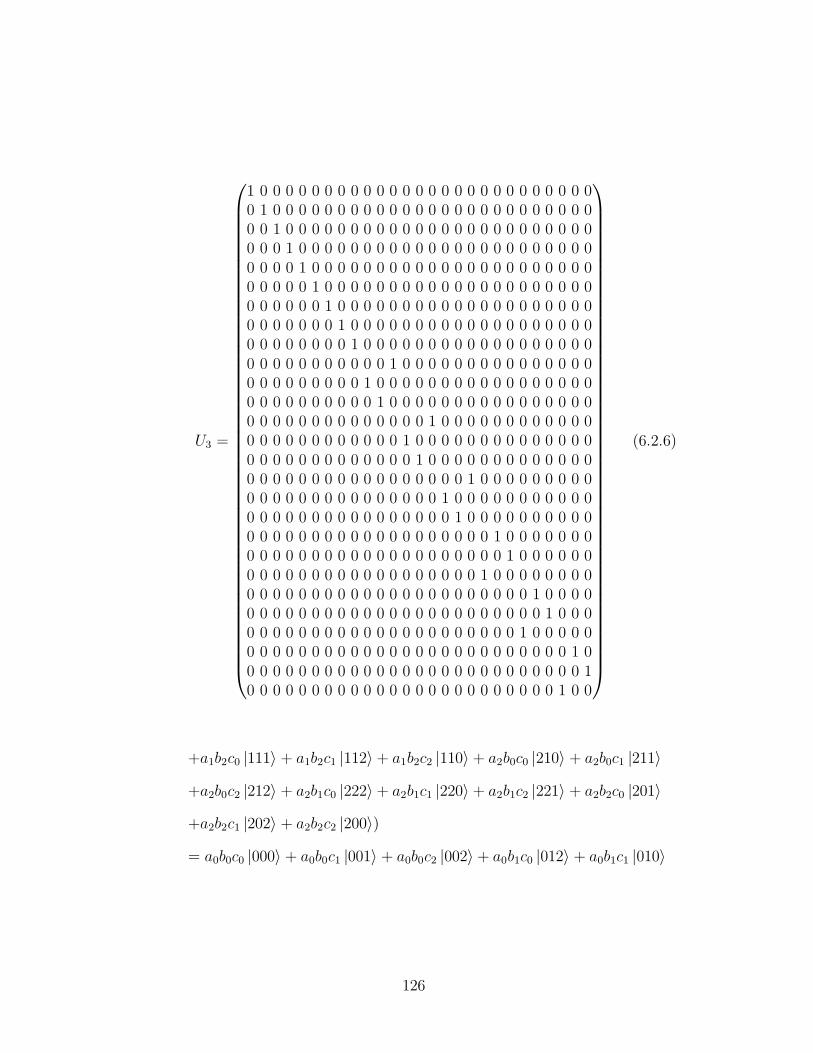
U3 =
1 0 0 0 0 0 0 0 0 0 0 0 0 0 0 0 0 0 0 0 0 0 0 0 0 0 00 1 0 0 0 0 0 0 0 0 0 0 0 0 0 0 0 0 0 0 0 0 0 0 0 0 00 0 1 0 0 0 0 0 0 0 0 0 0 0 0 0 0 0 0 0 0 0 0 0 0 0 00 0 0 1 0 0 0 0 0 0 0 0 0 0 0 0 0 0 0 0 0 0 0 0 0 0 00 0 0 0 1 0 0 0 0 0 0 0 0 0 0 0 0 0 0 0 0 0 0 0 0 0 00 0 0 0 0 1 0 0 0 0 0 0 0 0 0 0 0 0 0 0 0 0 0 0 0 0 00 0 0 0 0 0 1 0 0 0 0 0 0 0 0 0 0 0 0 0 0 0 0 0 0 0 00 0 0 0 0 0 0 1 0 0 0 0 0 0 0 0 0 0 0 0 0 0 0 0 0 0 00 0 0 0 0 0 0 0 1 0 0 0 0 0 0 0 0 0 0 0 0 0 0 0 0 0 00 0 0 0 0 0 0 0 0 0 0 1 0 0 0 0 0 0 0 0 0 0 0 0 0 0 00 0 0 0 0 0 0 0 0 1 0 0 0 0 0 0 0 0 0 0 0 0 0 0 0 0 00 0 0 0 0 0 0 0 0 0 1 0 0 0 0 0 0 0 0 0 0 0 0 0 0 0 00 0 0 0 0 0 0 0 0 0 0 0 0 0 1 0 0 0 0 0 0 0 0 0 0 0 00 0 0 0 0 0 0 0 0 0 0 0 1 0 0 0 0 0 0 0 0 0 0 0 0 0 00 0 0 0 0 0 0 0 0 0 0 0 0 1 0 0 0 0 0 0 0 0 0 0 0 0 00 0 0 0 0 0 0 0 0 0 0 0 0 0 0 0 0 1 0 0 0 0 0 0 0 0 00 0 0 0 0 0 0 0 0 0 0 0 0 0 0 1 0 0 0 0 0 0 0 0 0 0 00 0 0 0 0 0 0 0 0 0 0 0 0 0 0 0 1 0 0 0 0 0 0 0 0 0 00 0 0 0 0 0 0 0 0 0 0 0 0 0 0 0 0 0 0 1 0 0 0 0 0 0 00 0 0 0 0 0 0 0 0 0 0 0 0 0 0 0 0 0 0 0 1 0 0 0 0 0 00 0 0 0 0 0 0 0 0 0 0 0 0 0 0 0 0 0 1 0 0 0 0 0 0 0 00 0 0 0 0 0 0 0 0 0 0 0 0 0 0 0 0 0 0 0 0 0 1 0 0 0 00 0 0 0 0 0 0 0 0 0 0 0 0 0 0 0 0 0 0 0 0 0 0 1 0 0 00 0 0 0 0 0 0 0 0 0 0 0 0 0 0 0 0 0 0 0 0 1 0 0 0 0 00 0 0 0 0 0 0 0 0 0 0 0 0 0 0 0 0 0 0 0 0 0 0 0 0 1 00 0 0 0 0 0 0 0 0 0 0 0 0 0 0 0 0 0 0 0 0 0 0 0 0 0 10 0 0 0 0 0 0 0 0 0 0 0 0 0 0 0 0 0 0 0 0 0 0 0 1 0 0
(6.2.6)
+a1b2c0 |111〉 + a1b2c1 |112〉 + a1b2c2 |110〉 + a2b0c0 |210〉 + a2b0c1 |211〉
+a2b0c2 |212〉 + a2b1c0 |222〉 + a2b1c1 |220〉 + a2b1c2 |221〉 + a2b2c0 |201〉
+a2b2c1 |202〉 + a2b2c2 |200〉)
= a0b0c0 |000〉 + a0b0c1 |001〉 + a0b0c2 |002〉 + a0b1c0 |012〉 + a0b1c1 |010〉
126
+a0b1c2 |011〉 + a0b2c0 |021〉 + a0b2c1 |022〉 + a0b2c2 |020〉 + a1b0c0 |121〉
+a1b0c1 |122〉 + a1b0c2 |120〉 + a1b1c0 |100〉 + a1b1c1 |101〉 + a1b1c2 |102〉
+a1b2c0 |112〉 + a1b2c1 |110〉 + a1b2c2 |111〉 + a2b0c0 |212〉 + a2b0c1 |210〉
+a2b0c2 |211〉 + a2b1c0 |221〉 + a2b1c1 |222〉 + a2b1c2 |220〉 + a2b2c0 |200〉
+a2b2c1 |201〉 + a2b2c2 |202〉 . (6.2.7)
Let U4 and U5 be the unitary transformations given by U4(|ijk〉) = |(i+ j)jk〉
and U5(|ijk〉) = |i(j + k)k〉. Then Stage 4 of WilNOT is done by applying U4
and then U5. The results of applying U4 and U5 are
U4(a0b0c0 |000〉 + a0b0c1 |001〉 + a0b0c2 |002〉 + a0b1c0 |012〉 + a0b1c1 |010〉
+a0b1c2 |011〉 + a0b2c0 |021〉 + a0b2c1 |022〉 + a0b2c2 |020〉 + a1b0c0 |121〉
+a1b0c1 |122〉 + a1b0c2 |120〉 + a1b1c0 |100〉 + a1b1c1 |101〉 + a1b1c2 |102〉
+a1b2c0 |112〉 + a1b2c1 |110〉 + a1b2c2 |111〉 + a2b0c0 |212〉 + a2b0c1 |210〉
+a2b0c2 |211〉 + a2b1c0 |221〉 + a2b1c1 |222〉 + a2b1c2 |220〉 + a2b2c0 |200〉
+a2b2c1 |201〉 + a2b2c2 |202〉)
= a0b0c0 |000〉 + a0b0c1 |001〉 + a0b0c2 |002〉 + a0b1c0 |112〉 + a0b1c1 |110〉
+a0b1c2 |111〉 + a0b2c0 |221〉 + a0b2c1 |222〉 + a0b2c2 |220〉 + a1b0c0 |021〉
+a1b0c1 |022〉 + a1b0c2 |020〉 + a1b1c0 |100〉 + a1b1c1 |101〉 + a1b1c2 |102〉
+a1b2c0 |212〉 + a1b2c1 |210〉 + a1b2c2 |211〉 + a2b0c0 |012〉 + a2b0c1 |010〉
+a2b0c2 |011〉 + a2b1c0 |121〉 + a2b1c1 |122〉 + a2b1c2 |120〉 + a2b2c0 |200〉
+a2b2c1 |201〉 + a2b2c2 |202〉 (6.2.8)
and
U5(a0b0c0 |000〉 + a0b0c1 |001〉 + a0b0c2 |002〉 + a0b1c0 |112〉 + a0b1c1 |110〉
127
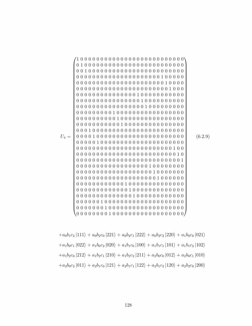
U4 =
1 0 0 0 0 0 0 0 0 0 0 0 0 0 0 0 0 0 0 0 0 0 0 0 0 0 00 1 0 0 0 0 0 0 0 0 0 0 0 0 0 0 0 0 0 0 0 0 0 0 0 0 00 0 1 0 0 0 0 0 0 0 0 0 0 0 0 0 0 0 0 0 0 0 0 0 0 0 00 0 0 0 0 0 0 0 0 0 0 0 0 0 0 0 0 0 0 0 0 1 0 0 0 0 00 0 0 0 0 0 0 0 0 0 0 0 0 0 0 0 0 0 0 0 0 0 1 0 0 0 00 0 0 0 0 0 0 0 0 0 0 0 0 0 0 0 0 0 0 0 0 0 0 1 0 0 00 0 0 0 0 0 0 0 0 0 0 0 0 0 0 1 0 0 0 0 0 0 0 0 0 0 00 0 0 0 0 0 0 0 0 0 0 0 0 0 0 0 1 0 0 0 0 0 0 0 0 0 00 0 0 0 0 0 0 0 0 0 0 0 0 0 0 0 0 1 0 0 0 0 0 0 0 0 00 0 0 0 0 0 0 0 0 1 0 0 0 0 0 0 0 0 0 0 0 0 0 0 0 0 00 0 0 0 0 0 0 0 0 0 1 0 0 0 0 0 0 0 0 0 0 0 0 0 0 0 00 0 0 0 0 0 0 0 0 0 0 1 0 0 0 0 0 0 0 0 0 0 0 0 0 0 00 0 0 1 0 0 0 0 0 0 0 0 0 0 0 0 0 0 0 0 0 0 0 0 0 0 00 0 0 0 1 0 0 0 0 0 0 0 0 0 0 0 0 0 0 0 0 0 0 0 0 0 00 0 0 0 0 1 0 0 0 0 0 0 0 0 0 0 0 0 0 0 0 0 0 0 0 0 00 0 0 0 0 0 0 0 0 0 0 0 0 0 0 0 0 0 0 0 0 0 0 0 1 0 00 0 0 0 0 0 0 0 0 0 0 0 0 0 0 0 0 0 0 0 0 0 0 0 0 1 00 0 0 0 0 0 0 0 0 0 0 0 0 0 0 0 0 0 0 0 0 0 0 0 0 0 10 0 0 0 0 0 0 0 0 0 0 0 0 0 0 0 0 0 1 0 0 0 0 0 0 0 00 0 0 0 0 0 0 0 0 0 0 0 0 0 0 0 0 0 0 1 0 0 0 0 0 0 00 0 0 0 0 0 0 0 0 0 0 0 0 0 0 0 0 0 0 0 1 0 0 0 0 0 00 0 0 0 0 0 0 0 0 0 0 0 1 0 0 0 0 0 0 0 0 0 0 0 0 0 00 0 0 0 0 0 0 0 0 0 0 0 0 1 0 0 0 0 0 0 0 0 0 0 0 0 00 0 0 0 0 0 0 0 0 0 0 0 0 0 1 0 0 0 0 0 0 0 0 0 0 0 00 0 0 0 0 0 1 0 0 0 0 0 0 0 0 0 0 0 0 0 0 0 0 0 0 0 00 0 0 0 0 0 0 1 0 0 0 0 0 0 0 0 0 0 0 0 0 0 0 0 0 0 00 0 0 0 0 0 0 0 1 0 0 0 0 0 0 0 0 0 0 0 0 0 0 0 0 0 0
(6.2.9)
+a0b1c2 |111〉 + a0b2c0 |221〉 + a0b2c1 |222〉 + a0b2c2 |220〉 + a1b0c0 |021〉
+a1b0c1 |022〉 + a1b0c2 |020〉 + a1b1c0 |100〉 + a1b1c1 |101〉 + a1b1c2 |102〉
+a1b2c0 |212〉 + a1b2c1 |210〉 + a1b2c2 |211〉 + a2b0c0 |012〉 + a2b0c1 |010〉
+a2b0c2 |011〉 + a2b1c0 |121〉 + a2b1c1 |122〉 + a2b1c2 |120〉 + a2b2c0 |200〉
128

U5 =
1 0 0 0 0 0 0 0 0 0 0 0 0 0 0 0 0 0 0 0 0 0 0 0 0 0 00 0 0 0 0 0 0 1 0 0 0 0 0 0 0 0 0 0 0 0 0 0 0 0 0 0 00 0 0 0 0 1 0 0 0 0 0 0 0 0 0 0 0 0 0 0 0 0 0 0 0 0 00 0 0 1 0 0 0 0 0 0 0 0 0 0 0 0 0 0 0 0 0 0 0 0 0 0 00 1 0 0 0 0 0 0 0 0 0 0 0 0 0 0 0 0 0 0 0 0 0 0 0 0 00 0 0 0 0 0 0 0 1 0 0 0 0 0 0 0 0 0 0 0 0 0 0 0 0 0 00 0 0 0 0 0 1 0 0 0 0 0 0 0 0 0 0 0 0 0 0 0 0 0 0 0 00 0 0 0 1 0 0 0 0 0 0 0 0 0 0 0 0 0 0 0 0 0 0 0 0 0 00 0 1 0 0 0 0 0 0 0 0 0 0 0 0 0 0 0 0 0 0 0 0 0 0 0 00 0 0 0 0 0 0 0 0 1 0 0 0 0 0 0 0 0 0 0 0 0 0 0 0 0 00 0 0 0 0 0 0 0 0 0 0 0 0 0 0 0 1 0 0 0 0 0 0 0 0 0 00 0 0 0 0 0 0 0 0 0 0 0 0 0 1 0 0 0 0 0 0 0 0 0 0 0 00 0 0 0 0 0 0 0 0 0 0 0 1 0 0 0 0 0 0 0 0 0 0 0 0 0 00 0 0 0 0 0 0 0 0 0 1 0 0 0 0 0 0 0 0 0 0 0 0 0 0 0 00 0 0 0 0 0 0 0 0 0 0 0 0 0 0 0 0 1 0 0 0 0 0 0 0 0 00 0 0 0 0 0 0 0 0 0 0 0 0 0 0 1 0 0 0 0 0 0 0 0 0 0 00 0 0 0 0 0 0 0 0 0 0 0 0 1 0 0 0 0 0 0 0 0 0 0 0 0 00 0 0 0 0 0 0 0 0 0 0 1 0 0 0 0 0 0 0 0 0 0 0 0 0 0 00 0 0 0 0 0 0 0 0 0 0 0 0 0 0 0 0 0 1 0 0 0 0 0 0 0 00 0 0 0 0 0 0 0 0 0 0 0 0 0 0 0 0 0 0 0 0 0 0 0 0 1 00 0 0 0 0 0 0 0 0 0 0 0 0 0 0 0 0 0 0 0 0 0 0 1 0 0 00 0 0 0 0 0 0 0 0 0 0 0 0 0 0 0 0 0 0 0 0 1 0 0 0 0 00 0 0 0 0 0 0 0 0 0 0 0 0 0 0 0 0 0 0 1 0 0 0 0 0 0 00 0 0 0 0 0 0 0 0 0 0 0 0 0 0 0 0 0 0 0 0 0 0 0 0 0 10 0 0 0 0 0 0 0 0 0 0 0 0 0 0 0 0 0 0 0 0 0 0 0 1 0 00 0 0 0 0 0 0 0 0 0 0 0 0 0 0 0 0 0 0 0 0 0 1 0 0 0 00 0 0 0 0 0 0 0 0 0 0 0 0 0 0 0 0 0 0 0 1 0 0 0 0 0 0
. (6.2.10)
+a2b2c1 |201〉 + a2b2c2 |202〉)
= a0b0c0 |000〉 + a0b0c1 |011〉 + a0b0c2 |022〉 + a0b1c0 |102〉 + a0b1c1 |110〉
+a0b1c2 |121〉 + a0b2c0 |201〉 + a0b2c1 |212〉 + a0b2c2 |220〉 + a1b0c0 |001〉
+a1b0c1 |012〉 + a1b0c2 |020〉 + a1b1c0 |100〉 + a1b1c1 |111〉 + a1b1c2 |122〉
129

+a1b2c0 |202〉 + a1b2c1 |210〉 + a1b2c2 |221〉 + a2b0c0 |002〉 + a2b0c1 |010〉
+a2b0c2 |021〉 + a2b1c0 |101〉 + a2b1c1 |112〉 + a2b1c2 |120〉 + a2b2c0 |200〉
+a2b2c1 |211〉 + a2b2c2 |222〉 . (6.2.11)
Let U6 and U7 be the unitary transformations given by U6(|ijk〉) = |ij(i+ k)〉
and U7(|ijk〉) = |ij(j + k)〉. Then Stage 5 of WilNOT is done by applying U6
and then applying U7 twice. The result of applying U6 is
U6(a0b0c0 |000〉 + a0b0c1 |011〉 + a0b0c2 |022〉 + a0b1c0 |102〉 + a0b1c1 |110〉
+a0b1c2 |121〉 + a0b2c0 |201〉 + a0b2c1 |212〉 + a0b2c2 |220〉 + a1b0c0 |001〉
+a1b0c1 |012〉 + a1b0c2 |020〉 + a1b1c0 |100〉 + a1b1c1 |111〉 + a1b1c2 |122〉
+a1b2c0 |202〉 + a1b2c1 |210〉 + a1b2c2 |221〉 + a2b0c0 |002〉 + a2b0c1 |010〉
+a2b0c2 |021〉 + a2b1c0 |101〉 + a2b1c1 |112〉 + a2b1c2 |120〉 + a2b2c0 |200〉
+a2b2c1 |211〉 + a2b2c2 |222〉)
= a0b0c0 |000〉 + a0b0c1 |011〉 + a0b0c2 |022〉 + a0b1c0 |100〉 + a0b1c1 |111〉
+a0b1c2 |122〉 + a0b2c0 |200〉 + a0b2c1 |211〉 + a0b2c2 |222〉 + a1b0c0 |001〉
+a1b0c1 |012〉 + a1b0c2 |020〉 + a1b1c0 |101〉 + a1b1c1 |112〉 + a1b1c2 |120〉
+a1b2c0 |201〉 + a1b2c1 |212〉 + a1b2c2 |220〉 + a2b0c0 |002〉 + a2b0c1 |010〉
+a2b0c2 |021〉 + a2b1c0 |102〉 + a2b1c1 |110〉 + a2b1c2 |121〉 + a2b2c0 |202〉
+a2b2c1 |210〉 + a2b2c2 |221〉 . (6.2.12)
Similarly, the action of U7 on the state 6.2.12 may be given as
U7(a0b0c0 |000〉 + a0b0c1 |011〉 + a0b0c2 |022〉 + a0b1c0 |100〉 + a0b1c1 |111〉
+a0b1c2 |122〉 + a0b2c0 |200〉 + a0b2c1 |211〉 + a0b2c2 |222〉 + a1b0c0 |001〉
+a1b0c1 |012〉 + a1b0c2 |020〉 + a1b1c0 |101〉 + a1b1c1 |112〉 + a1b1c2 |120〉
+a1b2c0 |201〉 + a1b2c1 |212〉 + a1b2c2 |220〉 + a2b0c0 |002〉 + a2b0c1 |010〉
130

+a2b0c2 |021〉 + a2b1c0 |102〉 + a2b1c1 |110〉 + a2b1c2 |121〉 + a2b2c0 |202〉
+a2b2c1 |210〉 + a2b2c2 |221〉)
= a0b0c0 |000〉 + a0b0c1 |012〉 + a0b0c2 |021〉 + a0b1c0 |100〉 + a0b1c1 |112〉
+a0b1c2 |121〉 + a0b2c0 |200〉 + a0b2c1 |212〉 + a0b2c2 |221〉 + a1b0c0 |001〉
+a1b0c1 |010〉 + a1b0c2 |022〉 + a1b1c0 |101〉 + a1b1c1 |110〉 + a1b1c2 |122〉
+a1b2c0 |201〉 + a1b2c1 |210〉 + a1b2c2 |222〉 + a2b0c0 |002〉 + a2b0c1 |011〉
+a2b0c2 |020〉 + a2b1c0 |102〉 + a2b1c1 |111〉 + a2b1c2 |120〉 + a2b2c0 |202〉
+a2b2c1 |211〉 + a2b2c2 |220〉 . (6.2.13)
The second application of U7 gives
U7(a0b0c0 |000〉 + a0b0c1 |012〉 + a0b0c2 |021〉 + a0b1c0 |100〉 + a0b1c1 |112〉
+a0b1c2 |121〉 + a0b2c0 |200〉 + a0b2c1 |212〉 + a0b2c2 |221〉 + a1b0c0 |001〉
+a1b0c1 |010〉 + a1b0c2 |022〉 + a1b1c0 |101〉 + a1b1c1 |110〉 + a1b1c2 |122〉
+a1b2c0 |201〉 + a1b2c1 |210〉 + a1b2c2 |222〉 + a2b0c0 |002〉 + a2b0c1 |011〉
+a2b0c2 |020〉 + a2b1c0 |102〉 + a2b1c1 |111〉 + a2b1c2 |120〉 + a2b2c0 |202〉
+a2b2c1 |211〉 + a2b2c2 |220〉)
= a0b0c0 |000〉 + a0b0c1 |010〉 + a0b0c2 |020〉 + a0b1c0 |100〉 + a0b1c1 |110〉
+a0b1c2 |120〉 + a0b2c0 |200〉 + a0b2c1 |210〉 + a0b2c2 |220〉 + a1b0c0 |001〉
+a1b0c1 |011〉 + a1b0c2 |021〉 + a1b1c0 |101〉 + a1b1c1 |111〉 + a1b1c2 |121〉
+a1b2c0 |201〉 + a1b2c1 |211〉 + a1b2c2 |221〉 + a2b0c0 |002〉 + a2b0c1 |012〉
+a2b0c2 |022〉 + a2b1c0 |102〉 + a2b1c1 |112〉 + a2b1c2 |122〉 + a2b2c0 |202〉
+a2b2c1 |212〉 + a2b2c2 |222〉 . (6.2.14)
The unitary matrices U6, and U7 have the following forms
131

U6 =
1 0 0 0 0 0 0 0 0 0 0 0 0 0 0 0 0 0 0 0 0 0 0 0 0 0 00 1 0 0 0 0 0 0 0 0 0 0 0 0 0 0 0 0 0 0 0 0 0 0 0 0 00 0 1 0 0 0 0 0 0 0 0 0 0 0 0 0 0 0 0 0 0 0 0 0 0 0 00 0 0 1 0 0 0 0 0 0 0 0 0 0 0 0 0 0 0 0 0 0 0 0 0 0 00 0 0 0 1 0 0 0 0 0 0 0 0 0 0 0 0 0 0 0 0 0 0 0 0 0 00 0 0 0 0 1 0 0 0 0 0 0 0 0 0 0 0 0 0 0 0 0 0 0 0 0 00 0 0 0 0 0 1 0 0 0 0 0 0 0 0 0 0 0 0 0 0 0 0 0 0 0 00 0 0 0 0 0 0 1 0 0 0 0 0 0 0 0 0 0 0 0 0 0 0 0 0 0 00 0 0 0 0 0 0 0 1 0 0 0 0 0 0 0 0 0 0 0 0 0 0 0 0 0 00 0 0 0 0 0 0 0 0 0 0 1 0 0 0 0 0 0 0 0 0 0 0 0 0 0 00 0 0 0 0 0 0 0 0 1 0 0 0 0 0 0 0 0 0 0 0 0 0 0 0 0 00 0 0 0 0 0 0 0 0 0 1 0 0 0 0 0 0 0 0 0 0 0 0 0 0 0 00 0 0 0 0 0 0 0 0 0 0 0 0 0 1 0 0 0 0 0 0 0 0 0 0 0 00 0 0 0 0 0 0 0 0 0 0 0 1 0 0 0 0 0 0 0 0 0 0 0 0 0 00 0 0 0 0 0 0 0 0 0 0 0 0 1 0 0 0 0 0 0 0 0 0 0 0 0 00 0 0 0 0 0 0 0 0 0 0 0 0 0 0 0 0 1 0 0 0 0 0 0 0 0 00 0 0 0 0 0 0 0 0 0 0 0 0 0 0 1 0 0 0 0 0 0 0 0 0 0 00 0 0 0 0 0 0 0 0 0 0 0 0 0 0 0 1 0 0 0 0 0 0 0 0 0 00 0 0 0 0 0 0 0 0 0 0 0 0 0 0 0 0 0 0 1 0 0 0 0 0 0 00 0 0 0 0 0 0 0 0 0 0 0 0 0 0 0 0 0 0 0 1 0 0 0 0 0 00 0 0 0 0 0 0 0 0 0 0 0 0 0 0 0 0 0 1 0 0 0 0 0 0 0 00 0 0 0 0 0 0 0 0 0 0 0 0 0 0 0 0 0 0 0 0 0 1 0 0 0 00 0 0 0 0 0 0 0 0 0 0 0 0 0 0 0 0 0 0 0 0 0 0 1 0 0 00 0 0 0 0 0 0 0 0 0 0 0 0 0 0 0 0 0 0 0 0 1 0 0 0 0 00 0 0 0 0 0 0 0 0 0 0 0 0 0 0 0 0 0 0 0 0 0 0 0 0 1 00 0 0 0 0 0 0 0 0 0 0 0 0 0 0 0 0 0 0 0 0 0 0 0 0 0 10 0 0 0 0 0 0 0 0 0 0 0 0 0 0 0 0 0 0 0 0 0 0 0 1 0 0
(6.2.15)
and
132

U7 =
1 0 0 0 0 0 0 0 0 0 0 0 0 0 0 0 0 0 0 0 0 0 0 0 0 0 00 1 0 0 0 0 0 0 0 0 0 0 0 0 0 0 0 0 0 0 0 0 0 0 0 0 00 0 1 0 0 0 0 0 0 0 0 0 0 0 0 0 0 0 0 0 0 0 0 0 0 0 00 0 0 0 0 1 0 0 0 0 0 0 0 0 0 0 0 0 0 0 0 0 0 0 0 0 00 0 0 1 0 0 0 0 0 0 0 0 0 0 0 0 0 0 0 0 0 0 0 0 0 0 00 0 0 0 1 0 0 0 0 0 0 0 0 0 0 0 0 0 0 0 0 0 0 0 0 0 00 0 0 0 0 0 0 1 0 0 0 0 0 0 0 0 0 0 0 0 0 0 0 0 0 0 00 0 0 0 0 0 0 0 1 0 0 0 0 0 0 0 0 0 0 0 0 0 0 0 0 0 00 0 0 0 0 0 1 0 0 0 0 0 0 0 0 0 0 0 0 0 0 0 0 0 0 0 00 0 0 0 0 0 0 0 0 1 0 0 0 0 0 0 0 0 0 0 0 0 0 0 0 0 00 0 0 0 0 0 0 0 0 0 1 0 0 0 0 0 0 0 0 0 0 0 0 0 0 0 00 0 0 0 0 0 0 0 0 0 0 1 0 0 0 0 0 0 0 0 0 0 0 0 0 0 00 0 0 0 0 0 0 0 0 0 0 0 0 0 1 0 0 0 0 0 0 0 0 0 0 0 00 0 0 0 0 0 0 0 0 0 0 0 1 0 0 0 0 0 0 0 0 0 0 0 0 0 00 0 0 0 0 0 0 0 0 0 0 0 0 1 0 0 0 0 0 0 0 0 0 0 0 0 00 0 0 0 0 0 0 0 0 0 0 0 0 0 0 0 1 0 0 0 0 0 0 0 0 0 00 0 0 0 0 0 0 0 0 0 0 0 0 0 0 0 0 1 0 0 0 0 0 0 0 0 00 0 0 0 0 0 0 0 0 0 0 0 0 0 0 1 0 0 0 0 0 0 0 0 0 0 00 0 0 0 0 0 0 0 0 0 0 0 0 0 0 0 0 0 1 0 0 0 0 0 0 0 00 0 0 0 0 0 0 0 0 0 0 0 0 0 0 0 0 0 0 1 0 0 0 0 0 0 00 0 0 0 0 0 0 0 0 0 0 0 0 0 0 0 0 0 0 0 1 0 0 0 0 0 00 0 0 0 0 0 0 0 0 0 0 0 0 0 0 0 0 0 0 0 0 0 0 1 0 0 00 0 0 0 0 0 0 0 0 0 0 0 0 0 0 0 0 0 0 0 0 1 0 0 0 0 00 0 0 0 0 0 0 0 0 0 0 0 0 0 0 0 0 0 0 0 0 0 1 0 0 0 00 0 0 0 0 0 0 0 0 0 0 0 0 0 0 0 0 0 0 0 0 0 0 0 0 1 00 0 0 0 0 0 0 0 0 0 0 0 0 0 0 0 0 0 0 0 0 0 0 0 0 0 10 0 0 0 0 0 0 0 0 0 0 0 0 0 0 0 0 0 0 0 0 0 0 0 1 0 0
. (6.2.16)
Note that state 6.2.14, the state of the system following the application of the
last unitary transformation as defined by WilNOT, can be written as
a0b0c0 |000〉 + a0b0c1 |010〉 + a0b0c2 |020〉 + a0b1c0 |100〉 + a0b1c1 |110〉
+a0b1c2 |120〉 + a0b2c0 |200〉 + a0b2c1 |210〉 + a0b2c2 |220〉 + a1b0c0 |001〉
+a1b0c1 |011〉 + a1b0c2 |021〉 + a1b1c0 |101〉 + a1b1c1 |111〉 + a1b1c2 |121〉
133
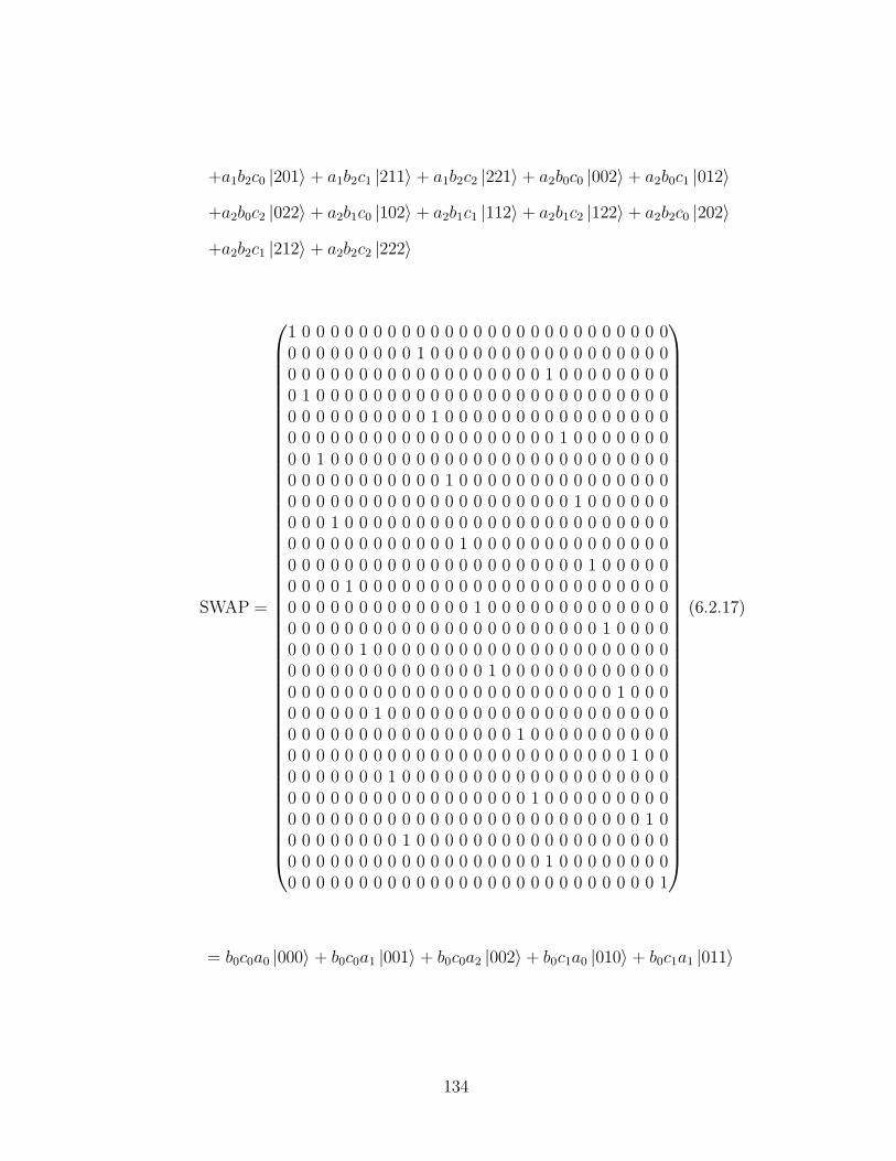
+a1b2c0 |201〉 + a1b2c1 |211〉 + a1b2c2 |221〉 + a2b0c0 |002〉 + a2b0c1 |012〉
+a2b0c2 |022〉 + a2b1c0 |102〉 + a2b1c1 |112〉 + a2b1c2 |122〉 + a2b2c0 |202〉
+a2b2c1 |212〉 + a2b2c2 |222〉
SWAP =
1 0 0 0 0 0 0 0 0 0 0 0 0 0 0 0 0 0 0 0 0 0 0 0 0 0 00 0 0 0 0 0 0 0 0 1 0 0 0 0 0 0 0 0 0 0 0 0 0 0 0 0 00 0 0 0 0 0 0 0 0 0 0 0 0 0 0 0 0 0 1 0 0 0 0 0 0 0 00 1 0 0 0 0 0 0 0 0 0 0 0 0 0 0 0 0 0 0 0 0 0 0 0 0 00 0 0 0 0 0 0 0 0 0 1 0 0 0 0 0 0 0 0 0 0 0 0 0 0 0 00 0 0 0 0 0 0 0 0 0 0 0 0 0 0 0 0 0 0 1 0 0 0 0 0 0 00 0 1 0 0 0 0 0 0 0 0 0 0 0 0 0 0 0 0 0 0 0 0 0 0 0 00 0 0 0 0 0 0 0 0 0 0 1 0 0 0 0 0 0 0 0 0 0 0 0 0 0 00 0 0 0 0 0 0 0 0 0 0 0 0 0 0 0 0 0 0 0 1 0 0 0 0 0 00 0 0 1 0 0 0 0 0 0 0 0 0 0 0 0 0 0 0 0 0 0 0 0 0 0 00 0 0 0 0 0 0 0 0 0 0 0 1 0 0 0 0 0 0 0 0 0 0 0 0 0 00 0 0 0 0 0 0 0 0 0 0 0 0 0 0 0 0 0 0 0 0 1 0 0 0 0 00 0 0 0 1 0 0 0 0 0 0 0 0 0 0 0 0 0 0 0 0 0 0 0 0 0 00 0 0 0 0 0 0 0 0 0 0 0 0 1 0 0 0 0 0 0 0 0 0 0 0 0 00 0 0 0 0 0 0 0 0 0 0 0 0 0 0 0 0 0 0 0 0 0 1 0 0 0 00 0 0 0 0 1 0 0 0 0 0 0 0 0 0 0 0 0 0 0 0 0 0 0 0 0 00 0 0 0 0 0 0 0 0 0 0 0 0 0 1 0 0 0 0 0 0 0 0 0 0 0 00 0 0 0 0 0 0 0 0 0 0 0 0 0 0 0 0 0 0 0 0 0 0 1 0 0 00 0 0 0 0 0 1 0 0 0 0 0 0 0 0 0 0 0 0 0 0 0 0 0 0 0 00 0 0 0 0 0 0 0 0 0 0 0 0 0 0 0 1 0 0 0 0 0 0 0 0 0 00 0 0 0 0 0 0 0 0 0 0 0 0 0 0 0 0 0 0 0 0 0 0 0 1 0 00 0 0 0 0 0 0 1 0 0 0 0 0 0 0 0 0 0 0 0 0 0 0 0 0 0 00 0 0 0 0 0 0 0 0 0 0 0 0 0 0 0 0 1 0 0 0 0 0 0 0 0 00 0 0 0 0 0 0 0 0 0 0 0 0 0 0 0 0 0 0 0 0 0 0 0 0 1 00 0 0 0 0 0 0 0 1 0 0 0 0 0 0 0 0 0 0 0 0 0 0 0 0 0 00 0 0 0 0 0 0 0 0 0 0 0 0 0 0 0 0 0 1 0 0 0 0 0 0 0 00 0 0 0 0 0 0 0 0 0 0 0 0 0 0 0 0 0 0 0 0 0 0 0 0 0 1
(6.2.17)
= b0c0a0 |000〉 + b0c0a1 |001〉 + b0c0a2 |002〉 + b0c1a0 |010〉 + b0c1a1 |011〉
134

+b0c1a2 |012〉 + b0c2a0 |020〉 + b0c2a1 |021〉 + b0c2a2 |022〉 + b1c0a0 |100〉
+b1c0a1 |101〉 + b1c0a2 |102〉 + b1c1a0 |110〉 + b1c1a1 |111〉 + b1c1a2 |112〉
+b1c2a0 |121〉 + b1c2a1 |121〉 + b1c2a2 |122〉 + b2c0a0 |200〉 + b2c0a1 |201〉
+b2c0a2 |202〉 + b2c1a0 |210〉 + b2c1a1 |211〉 + b2c1a2 |212〉 + b2c2a0 |220〉
+b2c2a1 |221〉 + b2c2a2 |222〉 . (6.2.18)
The state (6.2.18) is separable and has the form
(b0 |0〉 + b1 |1〉 + b2 |2〉)⊗ (c0 |0〉 + c1 |1〉 + c2 |2〉)⊗ (a0 |0〉 + a1 |1〉 + a2 |2〉)
= |b〉 ⊗ |c〉 ⊗ |a〉 , (6.2.19)
thereby illustrating WilNOT to be a quantum SWAP gate. Figure 6.8 gives
the WilNOT network for a qutrit SWAP of arbitrary quantum states. The
qutrit SWAP matrix for swapping the information content of three arbitrary
qutrit state is the product of the above transformations and is given by SWAP,
equation 6.2.17.
135

6.3 On the WilNOT Gate over Even
Dimensions Greater than Two
In this section, we consider the question of whether or not the WilNOT oper-
ator can be altered so that a generalised SWAP gate can be constructed over
even dimensions. This question is motivated by the case d = 4 in which we
considered if it was possible to swap the states of four 4-dimensional system
whereby first system A0 prepared in the state |e0〉0 is left in the state |e1〉0,
the second system A1 is prepared in the state |e1〉1 is left in the state |e2〉1, the
third system A2 prepared in the state |e2〉2 is left in the state |e3〉2 and finally
the system A3 prepared in the state |e3〉3 is left in the state |e0〉3. To this
end, let us consider an operator with Stage 1 and Stage 2 identical to those of
the WilNOT gate given in section 6.1. By (6.1.4) (with j = d − 1), at Stage
2 and step j = d − 1, the state of the algorithm is given by id−10 = i00, and
id−1k =
∑km=0
(k−m+d−2
d−2
)i0m for k = 1, . . . ,d − 1. To effectuate the algorithm
state (see (6.1.9) and (6.1.10))
i00(d− 1)i00 + i01
i00 + (d− 1)i01 + i02...
(d − 1)i00 + i01 + (d− 1)i02 + · · · + i0d−1
(6.3.1)
on systems A0, . . . ,Ad−1, the WilNOT algorithm process at Stage 3 for prime
d given in Section 6.1 requires revision when we consider dimensions d =
0 mod 2. Instead we take id−1k with the following linear combination
k−2∑
s=0
asid−1k−2−s =
k−2∑
s=0
as
(k−2)−s∑
m=0
((k − 2) − s−m+ d− 2
d − 2
)i0m
, (6.3.2)
where
as = d−
[(s+ 2 + d− 2
d− 2
)+
s−1∑
t=0
at
(s− t+ d− 2
d− 2
)]+ (−1)s,
136

. . .
. . .. . . . . .
. . .
. . . . . .
. . .
a0︷︸︸︷a0︷︸︸︷
a1︷︸︸︷
a0︷︸︸︷
a1︷︸︸︷
ad−4︷︸︸︷
ad−3︷︸︸︷
a2︷︸︸︷
t th h
h h hht t
ttt t
hhhhhh hhhh
tttt
tttt
. . .. . .
Figure 6.9: WilNOT gate over dimensions d = 0 mod 2; Stage 3.
and the result modulo d given by (6.3.1) can be obtained for Stage 3, step
j = d.
Theorem 21. For d = 0 mod 2, the algorithm process at Stage 3, step j = d
given by
idk = id−1k +
k−2∑
s=0
asid−1k−2−s
=k∑
m=0
(k −m+ d− 2
d − 2
)i0m +
k−2∑
s=0
as
(k−2)−s∑
m=0
((k − 2)− s−m+ d − 2
d− 2
)i0m
,
for k = 0, . . . ,d− 1, returns outcome (6.3.1).
Proof. For k = 0, 1, we have it that id0 = id−10 and id1 = id−1
1 . Thus, the
states e0 and e1 are given as i00 and (d− 1)i00 + i01 respectively. The state e2 is
written as
id2 =
2∑
m=0
(2−m+ d− 2
d− 2
)i0m + a0i
00
137

=
((d
d − 2
)+ (d−
(d
d− 2
)+ 1)
)i00 + (d− 1)i01 + i02
= (i00 + (d− 1)i01 + i02) mod d. (6.3.3)
We show by induction that, for k = 0 mod 2, idk =∑k
m=0
(k−m+d−2
d−2
)i0m +
∑k−2s=0
(as
∑(k−2)−sm=0
((k−2)−s−m+d−2
d−2
)i0m
)= i00+(d−1)i01+i
02+· · ·+(d−1)i0k−1+i
0k
modulo d and for k 6= 0 mod 2, idk = (d−1)i00+i01+(d−1)i02+· · ·+(d−1)i0k−1+i
0k
modulo d. We have shown that this is true for k = 0, 1, 2. Suppose 0 ≤ k ≤
d − 2 and further suppose that
idk =k∑
m=0
(k −m+ d− 2
d − 2
)i0m +
k−2∑
s=0
as
(k−2)−s∑
m=0
((k − 2)− s−m+ d − 2
d− 2
)i0m
=k∑
m=0
(−1)k−mi0m (6.3.4)
= (i00 + (d− 1)i01 + i02 + · · · + (d− 1)i0k−1 + i0k) mod d
for k = 0 mod 2, and
= ((d− 1)i00 + i01 + (d− 1)i02 + · · ·+ (d− 1)i0k−1 + i0k) mod d
for k 6= 0 mod 2. Therefore, for j = d, we have,
idk+1 =k+1∑
m=0
(k + 1−m+ d− 2
d− 2
)i0m +
k−1∑
s=0
as
(k−1)−s∑
m=0
((k − 1)− s−m+ d− 2
d− 2
)i0m
=k∑
m=0
((k −m+ d − 2
d− 2
)i0m+1 +
(k + 1 + d− 2
d− 2
)i00
)
+k−1∑
s=0
as
(k−2)−s∑
m=0
((k − 2)− s−m+ d − 2
d− 2
)i0m+1
+
((k − 1)− s+ d− 2
d− 2
)i00
=
k∑
m=0
(−1)k−mi0m+1 +
((k + 1 + d− 2
d− 2
)+
k−1∑
s=0
as
(k − 1− s+ d− 2
d− 2
))i00. (6.3.5)
Recall that the binomial coefficients of id−1k =
∑km=0
(k−m+d−2
d−2
)i0m are precisely
those coefficients of id−1k+1 =
∑k+1m=0
(k+1−m+d−2
d−2
)i0m for m = 1, . . . , k+ 1. Hence,
138

the particular combination of systems A(k−2)−s that return the state idk =
(i00 + (d − 1)i01 + i02 + · · · + (d − 1)i0k−1 + i0k) mod d is the combination that
effectuates a similar sequence on idk+1 for m = 1, . . . , k+1. Since k = 0 mod 2,
then for idk+1 we require that the scalar value for i00 degenerates to (d−1) mod
d. Thus, for m = 0 and by definition of as, we have((
(k + 1) + d− 2
d − 2
)+
k−1∑
s=0
as
((k − 1)− s+ d − 2
d− 2
))i00
=
(((k + 1) + d− 2
d− 2
)+
k−2∑
s=0
(as
((k − 1)− s+ d− 2
d− 2
))+ ak−1
)i00
=
(((k + 1) + d− 2
d− 2
)+
k−2∑
s=0
as
((k − 1)− s+ d− 2
d− 2
)
+
(d−
[((k + 1) + d − 2
d− 2
)+
k−2∑
s=0
as
((k − 1) − s+ d− 2
d− 2
)]+ (−1)k+1
))i00
= (−1)k+1i00. (6.3.6)
Hence, idk+1 =∑k+1
m=0 (−1)k+1−mi0m, and the result follows. We now implement
Stage 4 of the WilNOT gate, which is written as
id+1k = idk + idk+1 (6.3.7)
for k = 0, . . . ,d− 2 and
id+1d−1 = idd−1 +
d−2∑
m=0
(−1)d−1−si0m, (6.3.8)
and a revised Stage 5 given by∑d−1
k=1 η∗ki
d+2k =
∑bd−12
ct=0 (d − 1)i02t+1 +
∑d−22
t=0 i02t
which then returns
i01i02i03...
i0d−1
(d − 1)i00
. (6.3.9)
139

ξi0k
ξi0k+1 + ξi0k
i0k + (1 − ξ)i0k+1
ξi0k + ξi0k+1th
th
th
. . .
Figure 6.10: Pξ − 1 gates on pairs (ik, ik+1).
So, although we have not achieved our aim, our modification of the WilNOT
gate for d even has produced a similar state, namely a SWAP but with a
sign change for the system Ad−1. We have not been able to modify WilNOT
to produce the SWAP gate. We give the following argument to show that a
different approach would be required. Result (6.3.9) is a particular outcome
for an even valued d and once entered into this sequence of CNOTs seems not
to return an output with scalars on e0, . . . , ed−1 all equal to unity. To show
this claim, let us consider the more general case given by
ξi01ξi02ξi03...
ξi0d−1
(d− ξ)i00
. (6.3.10)
Consider the pairs (ξi0k, ξi0k+1), for k ∈ {1, . . . ,d−3}, and further consider the
pair (ξi0d−1, ξi00).
Given the paired input sequence (ξi0k, ξi0k+1), for k ∈ {1, . . . ,d − 3}, and
a mapping that targets ik+1, we have it that (ξi0k, ξi0k+1) 7→ (ξi0k, ξi
0k + ξi0k+1).
Denote by Pξ the inverse mod d of ξ, whence, Pξξ = 1 mod d. Applying
Pξ − 1 gates, see Figure 6.10, from the control with value ξi0k + ξi0k to the
140

i0k + (1 − ξ)i0k+1
ξi0k + ξi0k+1
i0k + (1 − ξ)i0k+1
ξ2i0k+1ht
ht
ht
. . .
Figure 6.11: d− ξ gates on (id−2, id−1).
target corresponding to the output ξi0k results in
(ξi0k, ξi0k + ξi0k+1) 7→ (Pξξi
0k + (Pξ − 1)ξi0k+1, ξi
0k + ξi0k+1)
= (i0k + (1 − ξ)i0k+1, ξi0k + ξi0k+1). (6.3.11)
To eliminate the value ξi0k from result (6.3.11), d − ξ gates are implemented
on the target ξi0k + ξi0k+1 thereby illustrating the mapping
(i0k + (1− ξ)i0k+1, ξi0k + ξi0k+1) 7→ (i0k + (1 − ξ)i0k+1, ξi
0k + ξi0k+1
+(d− ξ)(i0k + (1− ξ)i0k+1))
= (i0k + (1 − ξ)i0k+1, ξi0k+1
+(d− ξ)(1 − ξ)i0k+1))
= (i0k + (1 − ξ)i0k+1, ξi0k+1
+(−ξ + ξ2)i0k+1)
= (i0k + (1 − ξ)i0k+1, ξ2i0k+1). (6.3.12)
In a similar fashion, let us consider the final pair (ξid−1, (d− ξ)i0). Applying
those gates that correspond to result (6.3.11) and result (6.3.12) on the pair
ξid−1, (d − ξ)i0 returns the outcome (i0d−1 + (ξ − 1)i00,−ξ2i00). Thus, we have
141

the mapping given by
ξi01ξi02...
ξi0d−3
ξi0d−2
ξi0d−1
(d− ξ)i00
7→
i01 + (1− ξ)i02ξ2i02
...i0d−3 + (1− ξ)i0d−2
ξ2i0d−2
i0d−1 + (ξ − 1)i00−ξ2i00
. (6.3.13)
Since the scalar values ξ2 and −ξ2 can not simultaneously be unity, it seems
that any mapping on the state (6.3.10) will fail to return a state whose scalars
values all equal unity. That such outcome in result (6.3.13) is best possible
suggests that the WilNOT algorithm fails to extend over dimensions d =
0 mod 2. Therefore, it seems that WilNOT cannot be modified for the case
d even to permit a cycle of states such that first system A0 prepared in the
state |e0〉0 is left in the state |e1〉0, the second system A1 is prepared in the
state |e1〉1 is left in the state |e2〉1, the third system A2 prepared in the state
|e2〉2 is left in the state |e3〉2 and finally the system A3 prepared in the state
|e3〉3 is left in the state |e0〉3. Interestingly, WilNOT can demonstrate the case
where first system A0 prepared in the state |e0〉0 is left in the state |e2〉0, the
second system A1 is prepared in the state |e1〉1 is left in the state |e3〉1, the
third system A2 prepared in the state |e2〉2 is left in the state |e0〉2 and finally
the system A3 prepared in the state |e3〉3 is left in the state |e1〉3.
142

Chapter 7
On Binomial Summations andan Efficient GeneralisedQuantum SWAP Gate
Let us consider a set of d qudit quantum systems, the first system A0 prepared
in the state |e0〉0, the second systemA1 prepared in the state |e1〉1 and so forth,
with the final system Ad−1 prepared in the state |ed−1〉d−1. We ask whether or
not it is possible to construct a network to implement an efficient generalised
SWAP gate so that in the output of the network the system A0 is in the state
|e1〉0, the system A1 is in the state |e2〉1 and so forth, until the system Ad−1
is in the state |e0〉d−1 where e0, . . . , ed−1 ∈ {0, . . . ,d− 1}.
7.1 The Construction
Let k and l be positive integers. For non-negative integers j, the function
f(j) =(
jk
)mod l is a cyclic function of j [Lu, Tsai] [55]. We use the periodic
property of this function to study the computational problem associated with
the construction of an efficient generalised SWAP gate for quantum systems
over dimensions d. In particular, the binomial summation aj =∑j/d
i=0
(j−(d−1)i
i
)
mod d will be related to a quantum network for an efficient quantum gate,
143

aj (mod 4)︷ ︸︸ ︷
e1, e2, e3, e0, e0 ⊕ e1, . . .
x x y
0 0 0 1 1 1 1 2 3 0 1 3 2 2 3 2 0 2 1 3 3 1 2 1 0 1 3 0 0 1
1 0 0 0 1 1 1 1 2 3 0 1 3 2 2 3 2 0 2 1 3 3 1 2 1 0 1 3 0 0
0 1 0 0 0 1 1 1 1 2 3 0 1 3 2 2 3 2 0 2 1 3 3 1 2 1 0 1 3 0
0 0 1 0 0 0 1 1 1 1 2 3 0 1 3 2 2 3 2 0 2 1 3 3 1 2 1 0 1 3
e2
e1
e0
e3 . . .
. . .
. . .
. . .
ht
ht
th t
hht
ht
th t
hht
ht
th t
hht
ht
xy
Figure 7.1: Binomial summation Quantum SWAP network construction overdimension 4.
where such a network is constructed from by periodic application of CNOT
gates connecting adjacent systems of the network.
Figure 7.1 illustrates such a quantum netwrok for 4-dimensional quantum
states. The diagram shows the sequence of CNOT gates of the network. The
columns of the array on integers (modulo 4) describe the states of the target
systems after the corresponding CNOT gates have been applied, so the ar-
row indicates the correspondence between the system A1 being in the state
|e0 + e1〉1 (where e0 + e1 is calculated modulo 4) and the application of the
144

first CNOT gate. The sum e0 + e1 may be represented as the dot product of
the row vector e0, e1, e2, e3 and the corresponding column (1, 1, 0, 0)T . Thus
the array of integers (modulo 4) has rows indexed by {0, 1, 2, 3} and columns
indexed by (time t =) −3,−2,−1, 0, 1, 2, 3, . . . such that column t = 4s + j
with j ∈ {0, 1, 2, 3} corresponds to system Aj.
Denote the entries in the array by bit, where i ∈ {0, 1, 2, 3}, and t = −3,−2,
−1, 0, 1, 2, 3, . . . . Put at =∑3
i=0 e1bit, t = −3,−2,−1, 0, 1, 2, 3, . . . . Then, for
t = 4s+ j with j ∈ {0, 1, 2, 3}, the state of the system Aj is |a4s+j〉j ((Aj) has
been the target of s+ (1− δ0j) CNOT gates).
In general for a network of d systems (of dimension d), the periodic ar-
rangement of CNOT gates with control system Aj and target system Aj+1 for
j = 0, . . . ,d− 1 (where j+ 1 = 0 for j = d− 1) means that the sequence (at),
where |ads+j〉j is the state of systemA at time t = ds+j with j ∈ {0, . . . ,d−1}
and Aj has been the target of s + (1 − δ0j) CNOT gates, satisfies the recur-
rence at+d = at+d−1 + at for all t ≥ −d+ 1, since the CNOT gate replaces the
state |ads+j〉j of Aj with∣∣ad(s+1)+j
⟩j
=∣∣ads+j + ad(s+1)+j−1
⟩j. With initial
states |a−d+1〉1 = |e1〉1 , . . . , |a−1〉d−1 = |ed−1〉d−1, |a0〉0 = |e0〉0 the terms of
the sequence (at) may be written as at =∑d−1
i=0 eibit for sequences (bit) which
satisfy the recurrences bi(t+d) = bi(t+d−1) + bit, i = 0, . . . ,d− 1. Indeed
at+d−1 + at =
d−1∑
i=0
eibi(t+d−1) +
d−1∑
i=0
eibi(t)
=d−1∑
i=0
ei(bi(t+d−1) + bit) (7.1.1)
and
at+d =
d−1∑
i=0
eibi(t+d). (7.1.2)
We also note that, for i = 0, . . . ,d− 2 the sequence (bit) is a translate of the
145

sequence (b(i+1)t) by 1 place. (Indeed these sequences are all translates of one
another.)
We begin by considering the solution of the recurrence relation a(t+d) =
at+d−1 + at. This turns out to be at =∑t/d
i=0
(j−(d−1)
i
).
Lemma 4. [72](
xi
)+(
xi+1
)=(
x+1i+1
).
Lemma 5. Let d be a positive integer. The sequence 〈an〉 defined by an =∑n/d
i=0
(n−(d−1)i
i
)satisfies the recurrence relation an+d = an+d−1+an with initial
conditions a0 = · · · = ad−1 = 1.
Proof: Clearly the sequence 〈an〉 as defined satisfies a0 = · · · = ad−1 = 1.
Let l be a non-negative integer and let m ∈ {0, . . . ,d − 1}. Then ald+m
=∑l
i=0
((l−i)d+m+i
i
)and ald+m+d−1 = a(l+1)d+m−1 =
∑l+1i=0
((l+1−i)d+m+i−1
i
)
= 1 +∑l+1
i=1
((l+1−i)d+m+i−1
i
)= 1 +
∑li=0
((l−i)d+m+i
i+1
). Hence, by lemma 4,
ald+m + ald+m+d−1 = 1 +∑l
i=0
((l−i)d+m+i+1
i+1
)= 1 +
∑l+1i=1
((l+1−i)d+m+i
i
)=
∑l+1i=0
((l+1−i)d+m+i
i
)= a(l+1)d+m as required.
The solution sequence 〈aj〉 is periodic since the recurrence relation is re-
versible and the sequence must repeat as soon as d consecutive terms (of
which there are only finitely many possibilities) are repeated. To determine
the period we need some combinatorial results.
Lemma 6. [72]∑k
i=0
(j+ii
)=(
j+k+1k
)for all j ≥ 0.
Lemma 7. Let p be prime and let j ≥ −1. Then for j = p−1 (mod p), we have(
p+jp−1
)= 1(mod p) and for j = 0, . . . , p−2 (mod p), we have
(p+jp−1
)= 0 (mod p).
Proof: Let us write(
p+jp−1
)as a quotient of factorials, and consequently, we
have it that(
p+jp−1
)= (p+j)(p+j−1)...(p)
(j+1)!. There is a multiple of p in the numerator
not cancelled by a factor in the denominator except when j = p− 1 (mod p),
and the result follows.
146

Theorem 22. [55] Let p be a prime number and let a, and k be any positive
integers. The integer function(
jk
)modulo pa for j ≥ k has has the cycle length
pa+e where e = blogpkc.
We now determine the period of the solution sequence 〈aj〉 when d is prime.
Theorem 23. Let d be a prime and consider the sequence 〈aj〉 defined by
aj =∑j/d
i=0
(j−(d−1)i
i
)(mod d). Then 〈aj〉 has the cycle length d2 − 1.
Proof: The sequence 〈aj〉 satisfies the recurrence aj+d = aj+d−1 + aj for
all j. Since a0 = a1 = · · · = ad−1 = 1, it is sufficient to show that ad2−1 =
1, ad2−2 = 0, . . . , ad2−d = 0. This implies that aj+d2−1 = 1 for j = 0, . . . ,d−1,
and so aj+d2−1 = aj for all j ≥ 0. Now, for j = 0, . . . ,d− 2,
aj+d2−d =
j+d2−dd∑
i=0
(j + d2 − d− (d− 1)i
i
)
=d−1∑
i=0
(j + i
i
). (7.1.3)
By lemma 6,
d−1∑
i=0
(j + i
i
)=
(j + d
d− 1
)(mod d)
=
{0 mod d for 0 ≤ j < d− 11 mod d for j = d− 1.
(7.1.4)
Thus the period divides d2 − 1. Next, we show that Pa = d2 − 1 is the
smallest cycle length. For i = 0,(
j−(d−1)ii
)= 1 for all j ≥ 0. Let i be such
that 1 ≤ I < d2−1d
. Then the sequence (cj) with cj =(
j−(d−1)ii
)satisfies cj = 0
for j = 0, . . . ,di − 1 and cj = 1 for j = di and is periodic with period d for
j ≥ di by Theorem 22. Thus, ald = l + 1 for l = 0, . . . ,d − 1. Now any d
consecutive terms of a0, . . . , ad2−1 includes a term ald for some l and so cannot
147

be d− 1 consecutive zeroes and one 1 until the terms from d2 − d to d2 − 1.
This establishes the result.
Since the cycle length d2 − 1 is coprime to d at the completion of a cycle
the states of the system will be cycled round. Infact since d2 − 1 = d − 1 =
−1(mod d) they are shift by one position and the network implements the
SWAP gate – system A0 will be in the state |e1〉0, the initial state of A1, A1
will be in the state |e2〉1, . . . , Ad−1 will be in the state |e0〉d−1. This can be
seen by the following argument. Since the sequences 〈bit〉, i = 0, . . . ,d − 1,
have cycle length d2 − 1 we have (b0t, . . . , b(d−1)t) equal to: (0, 1, 0, . . . , 0) for
t = d2 − d corresponding to system A0; (0, 0, 1, 0, . . . , 0) for t = d2 − d + 1
corresponding to system A1; . . . ; (0, . . . , 0, 1) for t = d2 − 2 corresponding to
system Ad−2; (1, 0, . . . , 0) for t = d2 − 1 corresponding to system Ad−1.
7.1.1 The case d = pm
Now let us consider the prime power dimension d = pm with p prime and
let us further consider the family of binomial summations∑j/pm
i=0
(j−(pm−1)i
i
).
We conjecture that the cycle length of aj =∑j/pm
i=0
(j−(pm−1)i
i
)mod pm is
pm−1(p2m−1). We do not have a proof of this but we have written a computer
programme to calculate this value and have verified the conjecture for d =
4, 8, and 9; see Table 7.1. Note that if this conjecture is true then, since
gcd(pm, pm−1(p2m − 1)) = pm−1 6= 1, the network does not produce a SWAP
gate when m > 1. Although at the end of a cycle the systems are shifted
round, they are shifted pm−1 places and the systems return to their original
states after p applications of the network. Thus it provides a cyclic SWAP
on each of pm−1 groups of p systems, the systems of a group have indices
congruent modulo pm−1. What distinguishes this network from pm−1 copies of
the SWAP network for d = p is that in this larger network the systems that
148

are swapped do not actually directly interact through a CNOT gate.
We now consider the problem of determining the cycle length of the sequence
〈aj〉 for d = pm (m > 1). We have it that over such dimensions the sequence
〈aj〉 satifies the recurrence aj+pm = aj+pm−1 + aj for all j. Since a0 = a1 =
· · · = apm−1 = 1 by definition, it is sufficient to show that apm−1(p2m−1) = 1 and
apm−1(p2m−1)−j vanishes for j = 1, . . . , pm−1. It follows that apm−1(p2m−1)+j = 1
for j = 0, . . . , pm − 1. Following the approach for d = p we find that
apm−1(p2m−1)−j =
p2m−1−1∑
i=0
(pm−1(p2m − 1)− j − (pm − 1)i
i
)mod pm
=
p2m−1−1∑
i=0
((pm − 1)(p2m−1 + pm−1 − i)− j
i
)mod pm
=
p2m−1−1∑
i=0
((pm − 1)(pm−1 − i)− j
i
)mod pm
=
p2m−1−1∑
i=0
((1− pm)i− pm−1 − j
i
)mod pm. (7.1.5)
We ask the question if there exists a combinatorial approach which illustrates
that the sum∑p2m−1−1
i=0
((1−pm)i−pm−1−j
i
)mod pm equals 1 for j = 0 and vanishes
for j = 1, . . . , pm − 1. We have not been able to find an answer but outline
the approaches we have taken.
We now consider an alternative approach in evaluating the binomial sum-
mation aj =∑j/pm
i=0
(j−(pm−1)i
i
)mod pm. LetA(z) be the power series
∑j≥0 ajz
j
and denote by [zj]A(z) the coefficient of zj in A(z); thus [zj]A(z) = aj. We
now determine the generating function for A(z). A generating function is a
clothesline on which we hang up a sequence of numbers for display [94]. In
particular, the jth term of the sequence 〈aj〉 is the coefficient of zj in the
expansion of its generating function as a power series. To find the generat-
ing function associated the sequence 〈aj〉, we first note that the sequence 〈aj〉
149

satisfies the recurrence relation
aj =
0 if j < 01 if j = 0, . . . , pm − 1
aj−1 + aj−pm otherwise.(7.1.6)
This recurrence relation can be expressed as the single equation, we have
aj = aj−1 + aj−pm + [j = 0] (7.1.7)
where [j = 0] adds 1 when j = 0. To demonstrate the generating function for
A(z), we multiply both sides of (7.1.7) by zj and sum over j. Thus, we get
∞∑
j=0
ajzj =
∞∑
j=0
aj−1zj +
∞∑
j=0
aj−pmzj +∞∑
j=0
[j = 0]zj
=∞∑
j=0
ajzj+1 +
∞∑
j=0
ajzj+pm
+ 1
= z
∞∑
j=0
ajzj + zpm
∞∑
j=0
ajzj + 1. (7.1.8)
Consequently, the generating function for A(z) is given by 1/(1 − z − zpm).
Now, we can restate our problem to find a closed form for A(z), and thus
evaluate [zj]A(z). We use the following result from Graham et al. [35].
Lemma 8. [35] 1
(1−αz)i+1 =∑∞
n=0
(i+n
i
)αnzn.
We seek [zj]A(z) = [zj]1/(1 − z − zpm). Consider the series,
1/(1 − αz)i+1 =∞∑
j=0
(i+ j
i
)αjzj. (7.1.9)
Consider further a finite sum of such series;
S(z) =β1
(1 − α1z)i1+1
+ · · ·+ βN
(1− αNz)iN+1
. (7.1.10)
Then [zj]S(z) is the finite sum of coefficients given by
[zj]S(z) = β1
(i1 + j
i1
)αj
1 + · · ·+ βN
(iN + j
iN
)αj
N . (7.1.11)
150

Now, let A(z) = 1B(z)
where B(z) = 1 − z − zpm. We show that B(z) has
distinct roots. Let us suppose that B(z) has a set of repeated roots. Then,
we have it that B(z) and B′(z) share a set of common roots [68]. Since
B′(z) = −1 − pm(z)pm−1, it follows that a repeated root α satisfies B′(α) =
−1 − pm(α)pm−1 = 0, and consequently, αpm−1 = −1/pm. Whence, αpm=
−α/pm. Furthermore, as B(α) vanishes, we have it that 1 − α + α/pm = 0,
or equivalently, 1 − α(1 − 1/pm) = 0 from which we deduce α = pm/(pm − 1)
to be the only candidate for a repeating root. Therefore, α = pm/(pm − 1)
should satisfy the equation αpm−1 = −1/pm, as a consequence of being a
root of B′(z). That is (pm)pm−1
(pm−1)pm−1 = −1pm . Now (pm)pm ≡ 0 (mod p) while
−(pm − 1)pm−1 ≡ −1 (mod p) implies that α = pm/(pm − 1) is not a root of
B′(z). Therefore, B(z) has distinct roots.
Writing B(z) in the form (z − b1) . . . (z − bpm), and taking reciprocals
αk of bk, k = 1, . . . , pm, we establish a correspondence with the polynomial
(1 − α1z) . . . (1 − αpmz). Thus, A(z) = 1/((1 − α1z) . . . (1 − αpmz)) may take
the form β1/(1−α1z)+ · · ·+βpm/(1−αpmz), for some βl, l = 1, . . . , pm. Note
1/(1 − αz) is a special case of Lemma 8 with i = 0.
Theorem 24. We claim that
[zj]A(z) =
pm∑
l=1
βlαjl , (7.1.12)
where βl = −αl/B′(1/αl).
Proof:
limz→1/αl
(z − 1/αl)A(z) = limz→1/αl
(z − 1/αl)S(z), (7.1.13)
where S(z) is the special case of equation 7.1.11 with il = 0. Now, it follows
151
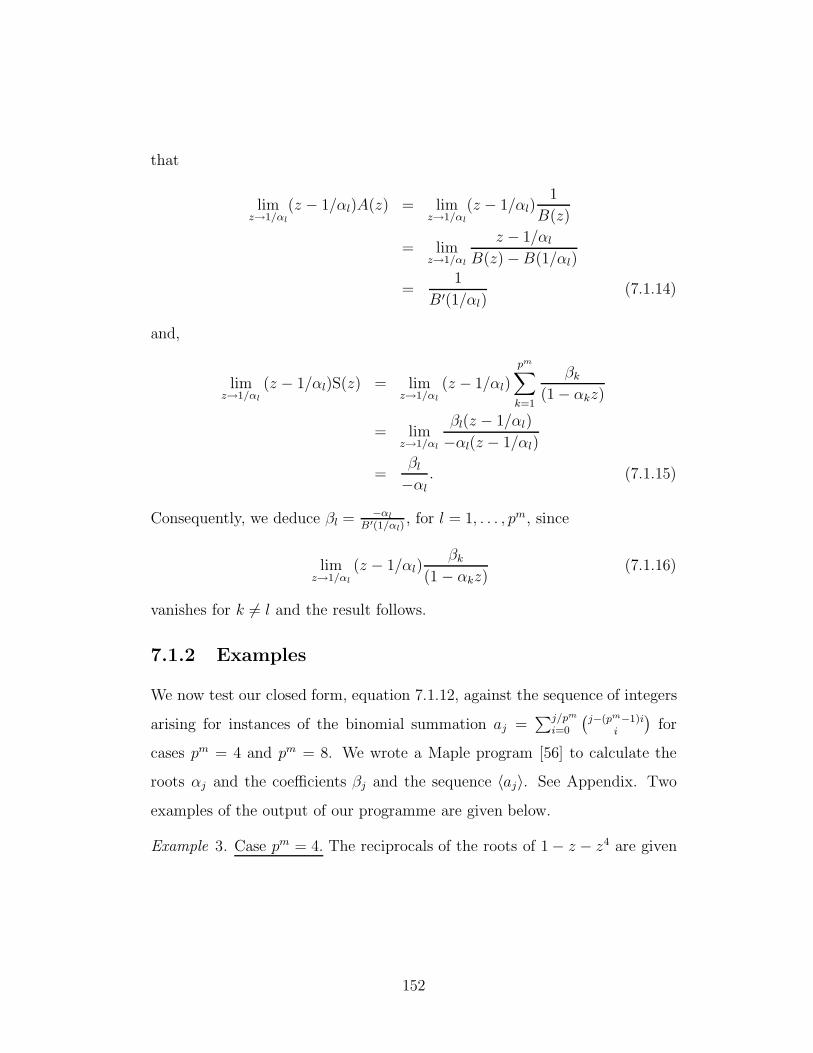
that
limz→1/αl
(z − 1/αl)A(z) = limz→1/αl
(z − 1/αl)1
B(z)
= limz→1/αl
z − 1/αl
B(z)−B(1/αl)
=1
B′(1/αl)(7.1.14)
and,
limz→1/αl
(z − 1/αl)S(z) = limz→1/αl
(z − 1/αl)
pm∑
k=1
βk
(1− αkz)
= limz→1/αl
βl(z − 1/αl)
−αl(z − 1/αl)
=βl
−αl. (7.1.15)
Consequently, we deduce βl = −αl
B′(1/αl), for l = 1, . . . , pm, since
limz→1/αl
(z − 1/αl)βk
(1 − αkz)(7.1.16)
vanishes for k 6= l and the result follows.
7.1.2 Examples
We now test our closed form, equation 7.1.12, against the sequence of integers
arising for instances of the binomial summation aj =∑j/pm
i=0
(j−(pm−1)i
i
)for
cases pm = 4 and pm = 8. We wrote a Maple program [56] to calculate the
roots αj and the coefficients βj and the sequence 〈aj〉. See Appendix. Two
examples of the output of our programme are given below.
Example 3. Case pm = 4. The reciprocals of the roots of 1− z − z4 are given
152

as
α1 = −.8191725134,
α2 = .219447421 − .9144736630ι,
α3 = .219447421 + .9144736630ι,
α4 = 1.380277569.
Since βl = −αl
B′(1/αl), we have
β1 = .1305102698,
β2 = .1610008758 + .1534011260ι,
β3 = .1610008758 − .1534011260ι,
β4 = .5474879784.
Following result (7.1.12), a closed form for the binomial coefficients aj is then
given by
aj = (.1305102698)(−.8191725134)j
+ (.1610 + .1534ι)(.2194 − .9144ι)j
+ (.1610 − .1534ι)(.2194 + .9144ι)j
+ (.5474879784)(1.380277569)j . (7.1.17)
Maple Input: for j from 0 to 25 do; aj; end;
Maple Output: 1,1,1,1,2,3,4,5,7,10,14,19,26,36,50,69,95,
131,181,250,345,476,657,907,1252,1728.
Example 4. Case pm = 8. The reciprocals of the roots of 1− z − z8 are given
153

as
α1 = −.9115923535,
α2 = −.6157823065 − .6871957511ι,
α3 = −.6157823065 + .6871957511ι,
α4 = .1033089835 − .9564836042ι
α5 = .1033089835 + .9564836042ι,
α6 = .8522421840 − .6352622030ι,
α7 = .8522421840 + .6352622030ι,
α8 = 1.232054631. (7.1.18)
The set βl, l = 1, . . . , 8, is
β1 = .06378010282,
β2 = .06449005934 + .02789285455ι,
β3 = .06449005934 − .02789285455ι,
β4 = .06911712233 + .06926484155ι,
β5 = .06911712233 − .06926484155ι,
β6 = .1188399306 + .1719523210ι,
β7 = .1188399306 − .1719523210ι,
β8 = .4313256714,
154

Again a closed form for the binomial coefficients aj is given by
aj = (.06378010282)(−.9115923535)j
+ (.0644 + .0278ι)(−.61578230 − .68719575ι)j
+ (.0644 − .0278ι)(−.61578230 + .68719575ι)j
+ (.0691 + .0692ι)(.10330898 − .95648360ι)j
+ (.0691 − .0692ι)(.10330898 + .95648360ι)j
+ (.1188 + .1719ι)(.85224218 − .63526220ι)j
+ (.1188 − .1719ι)(.85224218 + .63526220ι)j
+ (.4313256714)(1.232054631)j . (7.1.19)
Maple Input: for j from 0 to 25 do; aj; end;
Maple Output:1,1,1,1,1,1,1,1,2,3,4,5,6,7,8,9,11,14,18,23,29,
36,44,53,64,78.
7.2 On the cycle length of 〈aj mod pm〉
Having found a closed form for A(z) =∑
j≥0 ajzj, we now outline the classical
means by which the cycle length of 〈aj〉 mod pm may be determined.
The classical method: We fix a particular value of m > 1 and having
obtained the closed form for the coefficients of the corresponding polynomial
A(z), we evaluate the closed form of aj for j = 0, . . . , pm−1(p2m − 2). To
show that pm−1(p2m − 1) is the cycle length of 〈aj〉 mod pm, we show that
firstly apm−1(p2m−1) = 1 and apm−1(p2m−1)−j vanishes for j = 1, . . . , pm − 1, and
lastly, we show the subsequence of pm opening 1s does not appear until j is
pm−1(p2m − 1). While this proof follows the corresponding proof for the case
d = p, it differs in that Maple is required. Table 7.1 gives the cycle length of
155

the sequence 〈aj〉 for small values of pm. We have calculated the cycle length
for all prime powers up to 3125 and they all agree with the conjecture.
We now consider the sequence 〈aj〉 where aj =∑j/d
i=0
(j−(d−1)i
i
)mod d for
composite d with prime factorization d = pm11 . . . pmr
r . We may calculate the
cycle length of 〈aj〉 modulo d by calculating its cycle length modulo pmtt for
each t = 1, . . . , r. The cycle length of∑j/d
i=0
(j−(d−1)i
i
)mod pmt
t , for t = 1, . . . , r,
is given by the j for which∑j/d
i=1
(j−(d−1)i
i
)mod pmt
t equals 1 and which has
a preceding sequence (aj−d+1, . . . , aj−1) = (0, . . . , 0) mod pmtt . Given that the
mapping λd,(pm11 ...pmr
r ) : Zd 7→ Zpm11× · · · × Zpmr
ris well-defined then the cycle
length∣∣∣∑j/d
i=0
(j−(d−1)i
i
)mod d
∣∣∣ of the recurrence relation of 〈aj〉 is given by the
LCM{∣∣∣∑j/d
i=0
(j−(d−1)i
i
)mod pmt
t
∣∣∣}r
t=1. Table 7.1 gives some initial values for
the cycle length of∑j/d
i=0
(j−(d−1)i
i
)mod d. We state this result as a theorem.
Theorem 25. Let∑j/d
i=0
(j−(d−1)i
i
)mod d be an integer sequence and consider
the decomposition{∑j/d
i=0
(j−(d−1)i
i
)mod pmt
t
}r
t=1of∑j/d
i=0
(j−(d−1)i
i
)mod d into
a direct product of disjoint cycles. Let∣∣∣∑j/d
i=0
(j−(d−1)i
i
)mod d
∣∣∣ be the cycle
length of∑j/d
i=0
(j−(d−1)i
i
)mod d be and let
{∣∣∣∑j/d
i=0
(j−(d−1)i
i
)mod pmt
t
∣∣∣}r
t=1be
the cycle lengths of{∑j/d
i=0
(j−(d−1)i
i
)mod pmt
t
}r
t=1, respectively. Then, the
cycle length of∑j/d
i=0
(j−(d−1)i
i
)mod d is LCM
{∣∣∣∑j/d
i=0
(j−(d−1)i
i
)mod pmt
t
∣∣∣}r
t=1.
The results provided in Table 7.1 are the cycle lengths of aj for some small
values of d. The results are two-fold; firstly, the results give the minimum
number of CNOT gates required to effectuate a quantum gate according the
periodicity of the binomial summation construction. Secondly, use of the
binomial summation construction illustates for which dimensions the efficient
generalised SWAP gate can be realised. In particular, we have an efficient
SWAP gate in those dimensions d for which the cycle length of the function
aj is equivalent to −1 mod d. For dimensions d where our efficient SWAP
156

d∣∣∣∑j/d
i=0
(j−(d−1)i
i
)mod d
∣∣∣
2
3
4
5
6
7
8
9
3 = 22 − 1
8 = 32 − 1
30 = 2(24 − 1)
24 = 52 − 1
LCM(63, 728) = 6552
48 = 72 − 1
252 = 4(26 − 1)
240 = 3(34 − 1)
Table 7.1: Cycle length of∑j/d
i=0
(j−(d−1)i
i
)mod d.
157
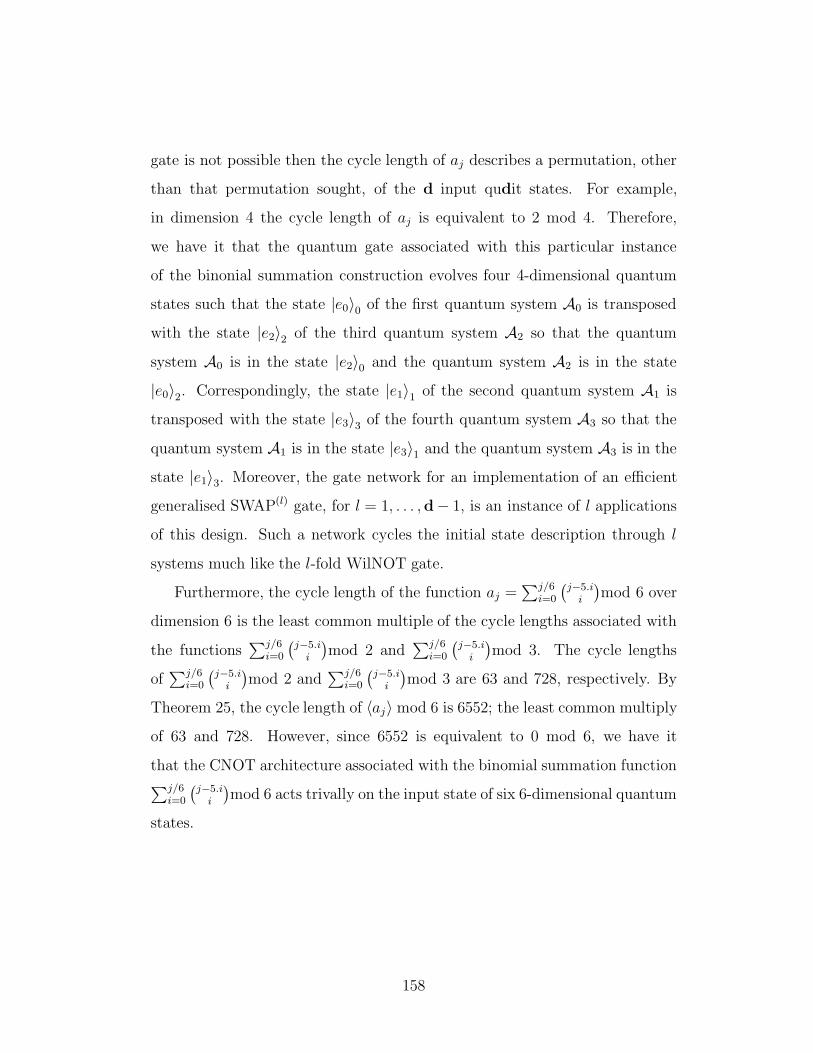
gate is not possible then the cycle length of aj describes a permutation, other
than that permutation sought, of the d input qudit states. For example,
in dimension 4 the cycle length of aj is equivalent to 2 mod 4. Therefore,
we have it that the quantum gate associated with this particular instance
of the binonial summation construction evolves four 4-dimensional quantum
states such that the state |e0〉0 of the first quantum system A0 is transposed
with the state |e2〉2 of the third quantum system A2 so that the quantum
system A0 is in the state |e2〉0 and the quantum system A2 is in the state
|e0〉2. Correspondingly, the state |e1〉1 of the second quantum system A1 is
transposed with the state |e3〉3 of the fourth quantum system A3 so that the
quantum system A1 is in the state |e3〉1 and the quantum system A3 is in the
state |e1〉3. Moreover, the gate network for an implementation of an efficient
generalised SWAP(l) gate, for l = 1, . . . ,d− 1, is an instance of l applications
of this design. Such a network cycles the initial state description through l
systems much like the l-fold WilNOT gate.
Furthermore, the cycle length of the function aj =∑j/6
i=0
(j−5.i
i
)mod 6 over
dimension 6 is the least common multiple of the cycle lengths associated with
the functions∑j/6
i=0
(j−5.i
i
)mod 2 and
∑j/6i=0
(j−5.i
i
)mod 3. The cycle lengths
of∑j/6
i=0
(j−5.i
i
)mod 2 and
∑j/6i=0
(j−5.i
i
)mod 3 are 63 and 728, respectively. By
Theorem 25, the cycle length of 〈aj〉 mod 6 is 6552; the least common multiply
of 63 and 728. However, since 6552 is equivalent to 0 mod 6, we have it
that the CNOT architecture associated with the binomial summation function∑j/6
i=0
(j−5.i
i
)mod 6 acts trivally on the input state of six 6-dimensional quantum
states.
158

|ψ〉2
|ψ〉1
|ψ〉0
|ψ〉0
|ψ〉2
|ψ〉1ht
ht
th
ht
ht
th
ht
ht
Figure 7.2: Quantum SWAP gate for qutrit states.
7.3 Efficient Qutrit SWAP
Earlier we gave an example of how the WilNOT network swapped the states
of three qutrits, see section 6.2. This quantum network based on the WilNOT
construction was composed of ten CNOT gates where addition was imple-
mented modulo 3. We improve on the WilNOT construction by considering a
construction based on binomial summations that yields a quantum gate which
is also composed entirely from uses of the CNOT gate. This new construction
is efficient in that it provides a construction of a generalised quantum SWAP
gate determined by fewest uses of the CNOT gate.
Figure 7.2 gives an efficient generalised quantum SWAP gate for qutrit
states which is based upon our binomial summation construction. As an in-
stance of Theorem 20, let us suppose that the first quantum system A0 pre-
pared in the state |e0〉0, the second system A1 prepared in the state |e1〉1 and
the third system A2 prepared in the state |e2〉2. Implementing our efficient
quantum SWAP gate yields the system A0 in the state |e1〉0, the system A1 is
in the state |e2〉1 and the system A2 is in the state |e0〉2 and this is achieved
with eight CNOT gates as aposed to the ten CNOT gates of the WilNOT
construction. Note further, that our efficient construction is based on a set of
binomial coefficients which satisfy the linear recurrence relation whose gener-
ating function is given by 1/(1−z−zpm). Generating functions provide elegant
159

means for the storing of information about the nature of coefficients in their
expansion [9]. For our purpose, the nature of the recurrence relation is seen
through periodicity of the coefficients modulo 3. We relate this periodic nature
to instances of the CNOT gate acting on basis states in determination of an
efficient quantum swap gate. Furthermore, since our quantum gate is based
on a linear recurrence relation, we illustrate that knowing part of quantum
gate design will completely aid in determining the remainder of the quantum
gate just as knowing the initial conditions of a recurrence relation determines
all other coefficients in the recurrence. Such type of construction is unusual
in that knowing part of the gate does not necessarily yield the remainder.
However, Nielsen [59] has proposed a similar idea to our binomial construc-
tion. In this construction, Nielsen maintains that knowing the initial position
and velocity of a geodesic, one can completely determine the remainder of the
geodesic by knowing its second order differential equation. Nielsen then main-
tains that such an equation describes the shortest path between the identity
operator and some quantum gate U . In this respect, our construction ideas
are similar; quantum gates can be constructed from knowing just particular
features of the gate. Our method is based on a combinatorial approach while
Nielsen considers efficient method through use of geodesics.
We now illustrate the action of each use of the generalised CNOT gate aris-
ing in our efficient construction on the input quantum states and subsequent
evolved states of the system. The first unitary gate U1 acts on the input state
of three arbitrary qutrits where the first quantum system A0 on the input
state is prepared in the state |e0〉0, the second system A1 on the input state
is prepared in the state |e1〉1 and the third system A2 on the input state is
160

prepared in the state |e2〉2. The action of U1 in the input state is given by
U1(|a〉 ⊗ |b〉 ⊗ |c〉)
= U1 ((a0 |0〉 + a1 |1〉 + a2 |2〉)⊗ (b0 |0〉+ b1 |1〉 + b2 |2〉)⊗ (c0 |0〉 + c1 |1〉+ c2 |2〉))
= U1(a0b0c0 |000〉 + a0b0c1 |001〉 + a0b0c2 |002〉 + a0b1c0 |010〉 + a0b1c1 |011〉
+a0b1c2 |012〉 + a0b2c0 |020〉 + a0b2c1 |021〉 + a0b2c2 |022〉 + a1b0c0 |100〉
U1 =
1 0 0 0 0 0 0 0 0 0 0 0 0 0 0 0 0 0 0 0 0 0 0 0 0 0 00 1 0 0 0 0 0 0 0 0 0 0 0 0 0 0 0 0 0 0 0 0 0 0 0 0 00 0 1 0 0 0 0 0 0 0 0 0 0 0 0 0 0 0 0 0 0 0 0 0 0 0 00 0 0 1 0 0 0 0 0 0 0 0 0 0 0 0 0 0 0 0 0 0 0 0 0 0 00 0 0 0 1 0 0 0 0 0 0 0 0 0 0 0 0 0 0 0 0 0 0 0 0 0 00 0 0 0 0 1 0 0 0 0 0 0 0 0 0 0 0 0 0 0 0 0 0 0 0 0 00 0 0 0 0 0 1 0 0 0 0 0 0 0 0 0 0 0 0 0 0 0 0 0 0 0 00 0 0 0 0 0 0 1 0 0 0 0 0 0 0 0 0 0 0 0 0 0 0 0 0 0 00 0 0 0 0 0 0 0 1 0 0 0 0 0 0 0 0 0 0 0 0 0 0 0 0 0 00 0 0 0 0 0 0 0 0 0 0 0 0 0 0 1 0 0 0 0 0 0 0 0 0 0 00 0 0 0 0 0 0 0 0 0 0 0 0 0 0 0 1 0 0 0 0 0 0 0 0 0 00 0 0 0 0 0 0 0 0 0 0 0 0 0 0 0 0 1 0 0 0 0 0 0 0 0 00 0 0 0 0 0 0 0 0 1 0 0 0 0 0 0 0 0 0 0 0 0 0 0 0 0 00 0 0 0 0 0 0 0 0 0 1 0 0 0 0 0 0 0 0 0 0 0 0 0 0 0 00 0 0 0 0 0 0 0 0 0 0 1 0 0 0 0 0 0 0 0 0 0 0 0 0 0 00 0 0 0 0 0 0 0 0 0 0 0 1 0 0 0 0 0 0 0 0 0 0 0 0 0 00 0 0 0 0 0 0 0 0 0 0 0 0 1 0 0 0 0 0 0 0 0 0 0 0 0 00 0 0 0 0 0 0 0 0 0 0 0 0 0 1 0 0 0 0 0 0 0 0 0 0 0 00 0 0 0 0 0 0 0 0 0 0 0 0 0 0 0 0 0 0 0 0 1 0 0 0 0 00 0 0 0 0 0 0 0 0 0 0 0 0 0 0 0 0 0 0 0 0 0 1 0 0 0 00 0 0 0 0 0 0 0 0 0 0 0 0 0 0 0 0 0 0 0 0 0 0 1 0 0 00 0 0 0 0 0 0 0 0 0 0 0 0 0 0 0 0 0 0 0 0 0 0 0 1 0 00 0 0 0 0 0 0 0 0 0 0 0 0 0 0 0 0 0 0 0 0 0 0 0 0 1 00 0 0 0 0 0 0 0 0 0 0 0 0 0 0 0 0 0 0 0 0 0 0 0 0 0 10 0 0 0 0 0 0 0 0 0 0 0 0 0 0 0 0 0 1 0 0 0 0 0 0 0 00 0 0 0 0 0 0 0 0 0 0 0 0 0 0 0 0 0 0 1 0 0 0 0 0 0 00 0 0 0 0 0 0 0 0 0 0 0 0 0 0 0 0 0 0 0 1 0 0 0 0 0 0
.
(7.3.1)
161

+a1b0c1 |101〉 + a1b0c2 |102〉 + a1b1c0 |110〉 + a1b1c1 |111〉 + a1b1c2 |112〉
+a1b2c0 |120〉 + a1b2c1 |121〉 + a1b2c2 |122〉 + a2b0c0 |200〉 + a2b0c1 |201〉
+a2b0c2 |202〉 + a2b1c0 |210〉 + a2b1c1 |211〉 + a2b1c2 |212〉 + a2b2c0 |220〉
+a2b2c1 |221〉 + a2b2c2 |222〉)
= a0b0c0 |000〉 + a0b0c1 |001〉 + a0b0c2 |002〉 + a0b1c0 |010〉 + a0b1c1 |011〉
+a0b1c2 |012〉 + a0b2c0 |020〉 + a0b2c1 |021〉 + a0b2c2 |022〉 + a1b0c0 |110〉
+a1b0c1 |111〉 + a1b0c2 |112〉 + a1b1c0 |120〉 + a1b1c1 |121〉 + a1b1c2 |122〉
+a1b2c0 |100〉 + a1b2c1 |101〉 + a1b2c2 |102〉 + a2b0c0 |220〉 + a2b0c1 |221〉
+a2b0c2 |222〉 + a2b1c0 |200〉 + a2b1c1 |201〉 + a2b1c2 |202〉 + a2b2c0 |210〉
+a2b2c1 |211〉 + a2b2c2 |212〉 . (7.3.2)
The second unitary matrix U2 corresponds to the second CNOT gate given
in Figure 7.2 and acts on the state of the system after application of the first
unitary transformation. The action of the unitary matrix U2 on the state of
the system
U1(a0b0c0 |000〉 + a0b0c1 |001〉 + a0b0c2 |002〉 + a0b1c0 |010〉 + a0b1c1 |011〉
+a0b1c2 |012〉 + a0b2c0 |020〉 + a0b2c1 |021〉 + a0b2c2 |022〉 + a1b0c0 |110〉
+a1b0c1 |111〉 + a1b0c2 |112〉 + a1b1c0 |120〉 + a1b1c1 |121〉 + a1b1c2 |122〉
+a1b2c0 |100〉 + a1b2c1 |101〉 + a1b2c2 |102〉 + a2b0c0 |220〉 + a2b0c1 |221〉
+a2b0c2 |222〉 + a2b1c0 |200〉 + a2b1c1 |201〉 + a2b1c2 |202〉 + a2b2c0 |210〉
+a2b2c1 |211〉 + a2b2c2 |212〉) (7.3.3)
is
U2(a0b0c0 |000〉 + a0b0c1 |001〉 + a0b0c2 |002〉 + a0b1c0 |010〉 + a0b1c1 |011〉
+a0b1c2 |012〉 + a0b2c0 |020〉 + a0b2c1 |021〉 + a0b2c2 |022〉 + a1b0c0 |110〉
162

U2 =
1 0 0 0 0 0 0 0 0 0 0 0 0 0 0 0 0 0 0 0 0 0 0 0 0 0 00 1 0 0 0 0 0 0 0 0 0 0 0 0 0 0 0 0 0 0 0 0 0 0 0 0 00 0 1 0 0 0 0 0 0 0 0 0 0 0 0 0 0 0 0 0 0 0 0 0 0 0 00 0 0 0 0 1 0 0 0 0 0 0 0 0 0 0 0 0 0 0 0 0 0 0 0 0 00 0 0 1 0 0 0 0 0 0 0 0 0 0 0 0 0 0 0 0 0 0 0 0 0 0 00 0 0 0 1 0 0 0 0 0 0 0 0 0 0 0 0 0 0 0 0 0 0 0 0 0 00 0 0 0 0 0 0 1 0 0 0 0 0 0 0 0 0 0 0 0 0 0 0 0 0 0 00 0 0 0 0 0 0 0 1 0 0 0 0 0 0 0 0 0 0 0 0 0 0 0 0 0 00 0 0 0 0 0 1 0 0 0 0 0 0 0 0 0 0 0 0 0 0 0 0 0 0 0 00 0 0 0 0 0 0 0 0 1 0 0 0 0 0 0 0 0 0 0 0 0 0 0 0 0 00 0 0 0 0 0 0 0 0 0 1 0 0 0 0 0 0 0 0 0 0 0 0 0 0 0 00 0 0 0 0 0 0 0 0 0 0 1 0 0 0 0 0 0 0 0 0 0 0 0 0 0 00 0 0 0 0 0 0 0 0 0 0 0 0 0 1 0 0 0 0 0 0 0 0 0 0 0 00 0 0 0 0 0 0 0 0 0 0 0 1 0 0 0 0 0 0 0 0 0 0 0 0 0 00 0 0 0 0 0 0 0 0 0 0 0 0 1 0 0 0 0 0 0 0 0 0 0 0 0 00 0 0 0 0 0 0 0 0 0 0 0 0 0 0 0 1 0 0 0 0 0 0 0 0 0 00 0 0 0 0 0 0 0 0 0 0 0 0 0 0 0 0 1 0 0 0 0 0 0 0 0 00 0 0 0 0 0 0 0 0 0 0 0 0 0 0 1 0 0 0 0 0 0 0 0 0 0 00 0 0 0 0 0 0 0 0 0 0 0 0 0 0 0 0 0 1 0 0 0 0 0 0 0 00 0 0 0 0 0 0 0 0 0 0 0 0 0 0 0 0 0 0 1 0 0 0 0 0 0 00 0 0 0 0 0 0 0 0 0 0 0 0 0 0 0 0 0 0 0 1 0 0 0 0 0 00 0 0 0 0 0 0 0 0 0 0 0 0 0 0 0 0 0 0 0 0 0 0 1 0 0 00 0 0 0 0 0 0 0 0 0 0 0 0 0 0 0 0 0 0 0 0 1 0 0 0 0 00 0 0 0 0 0 0 0 0 0 0 0 0 0 0 0 0 0 0 0 0 0 1 0 0 0 00 0 0 0 0 0 0 0 0 0 0 0 0 0 0 0 0 0 0 0 0 0 0 0 0 1 00 0 0 0 0 0 0 0 0 0 0 0 0 0 0 0 0 0 0 0 0 0 0 0 0 0 10 0 0 0 0 0 0 0 0 0 0 0 0 0 0 0 0 0 0 0 0 0 0 0 1 0 0
(7.3.4)
+a1b0c1 |111〉 + a1b0c2 |112〉 + a1b1c0 |120〉 + a1b1c1 |121〉 + a1b1c2 |122〉
+a1b2c0 |100〉 + a1b2c1 |101〉 + a1b2c2 |102〉 + a2b0c0 |220〉 + a2b0c1 |221〉
+a2b0c2 |222〉 + a2b1c0 |200〉 + a2b1c1 |201〉 + a2b1c2 |202〉 + a2b2c0 |210〉
+a2b2c1 |211〉 + a2b2c2 |212〉)
= a0b0c0 |000〉 + a0b0c1 |001〉 + a0b0c2 |002〉 + a0b1c0 |011〉 + a0b1c1 |012〉
163

+a0b1c2 |010〉 + a0b2c0 |022〉 + a0b2c1 |020〉 + a0b2c2 |021〉 + a1b0c0 |111〉
+a1b0c1 |112〉 + a1b0c2 |110〉 + a1b1c0 |122〉 + a1b1c1 |120〉 + a1b1c2 |121〉
+a1b2c0 |100〉 + a1b2c1 |101〉 + a1b2c2 |102〉 + a2b0c0 |222〉 + a2b0c1 |220〉
+a2b0c2 |221〉 + a2b1c0 |200〉 + a2b1c1 |201〉 + a2b1c2 |202〉 + a2b2c0 |211〉
+a2b2c1 |212〉 + a2b2c2 |210〉 . (7.3.5)
The unitary matrix U3 is given as
U3 =
1 0 0 0 0 0 0 0 0 0 0 0 0 0 0 0 0 0 0 0 0 0 0 0 0 0 00 0 0 0 0 0 0 0 0 0 0 0 0 0 0 0 0 0 0 1 0 0 0 0 0 0 00 0 0 0 0 0 0 0 0 0 0 1 0 0 0 0 0 0 0 0 0 0 0 0 0 0 00 0 0 1 0 0 0 0 0 0 0 0 0 0 0 0 0 0 0 0 0 0 0 0 0 0 00 0 0 0 0 0 0 0 0 0 0 0 0 0 0 0 0 0 0 0 0 0 1 0 1 0 00 0 0 0 0 0 0 0 0 0 0 0 0 0 1 0 0 0 0 0 0 0 0 0 0 0 00 0 0 0 0 0 1 0 0 0 0 0 0 0 0 0 0 0 0 0 0 0 0 0 0 0 00 0 0 0 0 0 0 0 0 0 0 0 0 0 0 0 0 0 0 0 0 0 0 0 0 1 00 0 0 0 0 0 0 0 0 0 0 0 0 0 0 0 0 1 0 0 0 0 0 0 0 0 00 0 0 0 0 0 0 0 0 1 0 0 0 0 0 0 0 0 0 0 0 0 0 0 0 0 00 0 0 0 0 0 0 0 0 0 0 0 0 0 0 0 0 0 0 0 0 0 0 0 0 0 00 0 1 0 0 0 0 0 0 0 0 0 0 0 0 0 0 0 0 0 1 0 0 0 0 0 00 0 0 0 0 0 0 0 0 0 0 0 1 0 0 0 0 0 0 0 0 0 0 0 0 0 00 0 0 0 1 0 0 0 0 0 0 0 0 0 0 0 0 0 0 0 0 0 0 0 0 0 00 0 0 0 0 0 0 0 0 0 0 0 0 0 0 0 0 0 0 0 0 0 0 1 0 0 00 0 0 0 0 0 0 0 0 0 0 0 0 0 0 1 0 0 0 0 0 0 0 0 0 0 00 0 0 0 0 0 0 1 0 0 0 0 0 0 0 0 0 0 0 0 0 0 0 0 0 0 00 0 0 0 0 0 0 0 0 0 0 0 0 0 0 0 0 0 0 0 0 0 0 0 0 0 10 0 0 0 0 0 0 0 0 0 0 0 0 0 0 0 0 0 1 0 0 0 0 0 0 0 00 1 0 0 0 0 0 0 0 0 1 0 0 0 0 0 0 0 0 0 0 0 0 0 0 0 00 0 0 0 0 0 0 0 0 0 0 0 0 0 0 0 0 0 0 0 0 0 0 0 0 0 00 0 0 0 0 0 0 0 0 0 0 0 0 0 0 0 0 0 0 0 0 1 0 0 0 0 00 0 0 0 0 0 0 0 0 0 0 0 0 1 0 0 0 0 0 0 0 0 0 0 0 0 00 0 0 0 0 1 0 0 0 0 0 0 0 0 0 0 0 0 0 0 0 0 0 0 0 0 00 0 0 0 0 0 0 0 0 0 0 0 0 0 0 0 0 0 0 0 0 0 0 0 1 0 00 0 0 0 0 0 0 0 0 0 0 0 0 0 0 0 1 0 0 0 0 0 0 0 0 0 00 0 0 0 0 0 0 0 1 0 0 0 0 0 0 0 0 0 0 0 0 0 0 0 0 0 0
(7.3.6)
The third unitary matrix U3 corresponds to the third CNOT gate given in
Figure 7.2 and acts on the state of the system after application of the second
164

unitary and its action on the state
U2U1(a0b0c0 |000〉 + a0b0c1 |001〉 + a0b0c2 |002〉 + a0b1c0 |010〉 + a0b1c1 |011〉
+a0b1c2 |012〉 + a0b2c0 |020〉 + a0b2c1 |021〉 + a0b2c2 |022〉 + a1b0c0 |110〉
+a1b0c1 |111〉 + a1b0c2 |112〉 + a1b1c0 |120〉 + a1b1c1 |121〉 + a1b1c2 |122〉
+a1b2c0 |100〉 + a1b2c1 |101〉 + a1b2c2 |102〉 + a2b0c0 |220〉 + a2b0c1 |221〉
+a2b0c2 |222〉 + a2b1c0 |200〉 + a2b1c1 |201〉 + a2b1c2 |202〉 + a2b2c0 |210〉
+a2b2c1 |211〉 + a2b2c2 |212〉) (7.3.7)
is
U3(a0b0c0 |000〉 + a0b0c1 |001〉 + a0b0c2 |002〉 + a0b1c0 |011〉 + a0b1c1 |012〉
+a0b1c2 |010〉 + a0b2c0 |022〉 + a0b2c1 |020〉 + a0b2c2 |021〉 + a1b0c0 |111〉
+a1b0c1 |112〉 + a1b0c2 |110〉 + a1b1c0 |122〉 + a1b1c1 |120〉 + a1b1c2 |121〉
+a1b2c0 |100〉 + a1b2c1 |101〉 + a1b2c2 |102〉 + a2b0c0 |222〉 + a2b0c1 |220〉
+a2b0c2 |221〉 + a2b1c0 |200〉 + a2b1c1 |201〉 + a2b1c2 |202〉 + a2b2c0 |211〉
+a2b2c1 |212〉 + a2b2c2 |210〉)
= a0b0c0 |000〉 + a0b0c1 |101〉 + a0b0c2 |202〉 + a0b1c0 |111〉 + a0b1c1 |212〉
+a0b1c2 |010〉 + a0b2c0 |222〉 + a0b2c1 |020〉 + a0b2c2 |121〉 + a1b0c0 |211〉
+a1b0c1 |012〉 + a1b0c2 |110〉 + a1b1c0 |022〉 + a1b1c1 |120〉 + a1b1c2 |221〉
+a1b2c0 |100〉 + a1b2c1 |201〉 + a1b2c2 |002〉 + a2b0c0 |122〉 + a2b0c1 |220〉
+a2b0c2 |021〉 + a2b1c0 |200〉 + a2b1c1 |001〉 + a2b1c2 |102〉 + a2b2c0 |011〉
+a2b2c1 |112〉 + a2b2c2 |210〉 . (7.3.8)
As outlined, this construction is based on a linear recurrence relation and
therefore there is a cyclic nature to our gate construction. This is evident
when we consider our gate within the qutrit setting. As such, our construction
165

is based upon repeat application of the unitrary matrices U1, U2, and U3. As
evident in Figure 7.2 the forth gate in the construction corresponds to the
unitary matrix U1. In particular, we have it that
U4(U3U2U1(a0b0c0 |000〉 + a0b0c1 |001〉 + a0b0c2 |002〉 + a0b1c0 |010〉 + a0b1c1 |011〉
+a0b1c2 |012〉 + a0b2c0 |020〉 + a0b2c1 |021〉 + a0b2c2 |022〉 + a1b0c0 |110〉
+a1b0c1 |111〉 + a1b0c2 |112〉 + a1b1c0 |120〉 + a1b1c1 |121〉 + a1b1c2 |122〉
+a1b2c0 |100〉 + a1b2c1 |101〉 + a1b2c2 |102〉 + a2b0c0 |220〉 + a2b0c1 |221〉
+a2b0c2 |222〉 + a2b1c0 |200〉 + a2b1c1 |201〉 + a2b1c2 |202〉 + a2b2c0 |210〉
+a2b2c1 |211〉 + a2b2c2 |212〉))
= U4(a0b0c0 |000〉 + a0b0c1 |101〉 + a0b0c2 |202〉 + a0b1c0 |111〉 + a0b1c1 |212〉
+a0b1c2 |010〉 + a0b2c0 |222〉 + a0b2c1 |020〉 + a0b2c2 |121〉 + a1b0c0 |211〉
+a1b0c1 |012〉 + a1b0c2 |110〉 + a1b1c0 |022〉 + a1b1c1 |120〉 + a1b1c2 |221〉
+a1b2c0 |100〉 + a1b2c1 |201〉 + a1b2c2 |002〉 + a2b0c0 |122〉 + a2b0c1 |220〉
+a2b0c2 |021〉 + a2b1c0 |200〉 + a2b1c1 |001〉 + a2b1c2 |102〉 + a2b2c0 |011〉
+a2b2c1 |112〉 + a2b2c2 |210〉)
= a0b0c0 |000〉 + a0b0c1 |111〉 + a0b0c2 |222〉 + a0b1c0 |121〉 + a0b1c1 |202〉
+a0b1c2 |010〉 + a0b2c0 |212〉 + a0b2c1 |020〉 + a0b2c2 |101〉 + a1b0c0 |201〉
+a1b0c1 |012〉 + a1b0c2 |120〉 + a1b1c0 |022〉 + a1b1c1 |100〉 + a1b1c2 |211〉
+a1b2c0 |110〉 + a1b2c1 |221〉 + a1b2c2 |002〉 + a2b0c0 |102〉 + a2b0c1 |210〉
+a2b0c2 |021〉 + a2b1c0 |220〉 + a2b1c1 |001〉 + a2b1c2 |112〉 + a2b2c0 |011〉
+a2b2c1 |122〉 + a2b2c2 |200〉 . (7.3.9)
In a similar fashion, we have it that
U5(U4U3U2U1(a0b0c0 |000〉 + a0b0c1 |001〉 + a0b0c2 |002〉 + a0b1c0 |010〉
166

+a0b1c1 |011〉 + a0b1c2 |012〉 + a0b2c0 |020〉 + a0b2c1 |021〉 + a0b2c2 |022〉
+a1b0c0 |110〉 + a1b0c1 |111〉 + a1b0c2 |112〉 + a1b1c0 |120〉 + a1b1c1 |121〉
+a1b1c2 |122〉 + a1b2c0 |100〉 + a1b2c1 |101〉 + a1b2c2 |102〉 + a2b0c0 |220〉
+a2b0c1 |221〉 + a2b0c2 |222〉 + a2b1c0 |200〉 + a2b1c1 |201〉 + a2b1c2 |202〉
+a2b2c0 |210〉 + a2b2c1 |211〉 + a2b2c2 |212〉))
= U5(a0b0c0 |000〉 + a0b0c1 |111〉 + a0b0c2 |222〉 + a0b1c0 |121〉 + a0b1c1 |202〉
+a0b1c2 |010〉 + a0b2c0 |212〉 + a0b2c1 |020〉 + a0b2c2 |101〉 + a1b0c0 |201〉
+a1b0c1 |012〉 + a1b0c2 |120〉 + a1b1c0 |022〉 + a1b1c1 |100〉 + a1b1c2 |211〉
+a1b2c0 |110〉 + a1b2c1 |221〉 + a1b2c2 |002〉 + a2b0c0 |102〉 + a2b0c1 |210〉
+a2b0c2 |021〉 + a2b1c0 |220〉 + a2b1c1 |001〉 + a2b1c2 |112〉 + a2b2c0 |011〉
+a2b2c1 |122〉 + a2b2c2 |200〉)
= a0b0c0 |000〉 + a0b0c1 |112〉 + a0b0c2 |221〉 + a0b1c0 |120〉 + a0b1c1 |202〉
+a0b1c2 |011〉 + a0b2c0 |210〉 + a0b2c1 |022〉 + a0b2c2 |101〉 + a1b0c0 |201〉
+a1b0c1 |010〉 + a1b0c2 |122〉 + a1b1c0 |021〉 + a1b1c1 |100〉 + a1b1c2 |212〉
+a1b2c0 |111〉 + a1b2c1 |220〉 + a1b2c2 |002〉 + a2b0c0 |102〉 + a2b0c1 |211〉
+a2b0c2 |020〉 + a2b1c0 |222〉 + a2b1c1 |001〉 + a2b1c2 |110〉 + a2b2c0 |012〉
+a2b2c1 |121〉 + a2b2c2 |200〉 (7.3.10)
where the unitary matrix U5 is given by the matrix U2. The next unitary
matrix U6, and as illustrated in Figure 7.2, given by this construction is the
matrix which corresponds to the matrix U3. We then have it that
U6(U5U4U3U2U1(a0b0c0 |000〉 + a0b0c1 |001〉 + a0b0c2 |002〉 + a0b1c0 |010〉
+a0b1c1 |011〉 + a0b1c2 |012〉 + a0b2c0 |020〉 + a0b2c1 |021〉 + a0b2c2 |022〉
167

+a1b0c0 |110〉 + a1b0c1 |111〉 + a1b0c2 |112〉 + a1b1c0 |120〉 + a1b1c1 |121〉
+a1b1c2 |122〉 + a1b2c0 |100〉 + a1b2c1 |101〉 + a1b2c2 |102〉 + a2b0c0 |220〉
+a2b0c1 |221〉 + a2b0c2 |222〉 + a2b1c0 |200〉 + a2b1c1 |201〉 + a2b1c2 |202〉
+a2b2c0 |210〉 + a2b2c1 |211〉 + a2b2c2 |212〉))
= U6(a0b0c0 |000〉 + a0b0c1 |112〉 + a0b0c2 |221〉 + a0b1c0 |120〉 + a0b1c1 |202〉
+a0b1c2 |011〉 + a0b2c0 |210〉 + a0b2c1 |022〉 + a0b2c2 |101〉 + a1b0c0 |201〉
+a1b0c1 |010〉 + a1b0c2 |122〉 + a1b1c0 |021〉 + a1b1c1 |100〉 + a1b1c2 |212〉
+a1b2c0 |111〉 + a1b2c1 |220〉 + a1b2c2 |002〉 + a2b0c0 |102〉 + a2b0c1 |211〉
+a2b0c2 |020〉 + a2b1c0 |222〉 + a2b1c1 |001〉 + a2b1c2 |110〉 + a2b2c0 |012〉
+a2b2c1 |121〉 + a2b2c2 |200〉)
= a0b0c0 |000〉 + a0b0c1 |012〉 + a0b0c2 |021〉 + a0b1c0 |120〉 + a0b1c1 |102〉
+a0b1c2 |111〉 + a0b2c0 |210〉 + a0b2c1 |222〉 + a0b2c2 |201〉 + a1b0c0 |001〉
+a1b0c1 |010〉 + a1b0c2 |022〉 + a1b1c0 |121〉 + a1b1c1 |100〉 + a1b1c2 |112〉
+a1b2c0 |211〉 + a1b2c1 |220〉 + a1b2c2 |202〉 + a2b0c0 |002〉 + a2b0c1 |011〉
+a2b0c2 |020〉 + a2b1c0 |122〉 + a2b1c1 |101〉 + a2b1c2 |110〉 + a2b2c0 |212〉
+a2b2c1 |221〉 + a2b2c2 |200〉 . (7.3.11)
Similarly,
U7(U6U5U4U3U2U1(a0b0c0 |000〉 + a0b0c1 |001〉 + a0b0c2 |002〉 + a0b1c0 |010〉
+a0b1c1 |011〉 + a0b1c2 |012〉 + a0b2c0 |020〉 + a0b2c1 |021〉 + a0b2c2 |022〉
+a1b0c0 |110〉 + a1b0c1 |111〉 + a1b0c2 |112〉 + a1b1c0 |120〉 + a1b1c1 |121〉
+a1b1c2 |122〉 + a1b2c0 |100〉 + a1b2c1 |101〉 + a1b2c2 |102〉 + a2b0c0 |220〉
+a2b0c1 |221〉 + a2b0c2 |222〉 + a2b1c0 |200〉 + a2b1c1 |201〉 + a2b1c2 |202〉
+a2b2c0 |210〉 + a2b2c1 |211〉 + a2b2c2 |212〉))
168

= U7(a0b0c0 |000〉 + a0b0c1 |012〉 + a0b0c2 |021〉 + a0b1c0 |120〉 + a0b1c1 |102〉
+a0b1c2 |111〉 + a0b2c0 |210〉 + a0b2c1 |222〉 + a0b2c2 |201〉 + a1b0c0 |001〉
+a1b0c1 |010〉 + a1b0c2 |022〉 + a1b1c0 |121〉 + a1b1c1 |100〉 + a1b1c2 |112〉
+a1b2c0 |211〉 + a1b2c1 |220〉 + a1b2c2 |202〉 + a2b0c0 |002〉 + a2b0c1 |011〉
+a2b0c2 |020〉 + a2b1c0 |122〉 + a2b1c1 |101〉 + a2b1c2 |110〉 + a2b2c0 |212〉
+a2b2c1 |221〉 + a2b2c2 |200〉)
= a0b0c0 |000〉 + a0b0c1 |012〉 + a0b0c2 |021〉 + a0b1c0 |100〉 + a0b1c1 |112〉
+a0b1c2 |121〉 + a0b2c0 |200〉 + a0b2c1 |212〉 + a0b2c2 |221〉 + a1b0c0 |001〉
+a1b0c1 |010〉 + a1b0c2 |022〉 + a1b1c0 |101〉 + a1b1c1 |110〉 + a1b1c2 |122〉
+a1b2c0 |201〉 + a1b2c1 |210〉 + a1b2c2 |222〉 + a2b0c0 |002〉 + a2b0c1 |011〉
+a2b0c2 |020〉 + a2b1c0 |102〉 + a2b1c1 |111〉 + a2b1c2 |120〉 + a2b2c0 |202〉
+a2b2c1 |211〉 + a2b2c2 |220〉 (7.3.12)
where the unitary matrix U7 is the matrix given by U1. Our final gate as
outlined in this contruction and evident in Figure 7.2 is the unitary matrix
U8. The unitary matrix U8 corresponds to the unitary matrix U2, and we have
U8(U7U6U5U4U3U2U1(a0b0c0 |000〉 + a0b0c1 |001〉 + a0b0c2 |002〉 + a0b1c0 |010〉
+a0b1c1 |011〉 + a0b1c2 |012〉 + a0b2c0 |020〉 + a0b2c1 |021〉 + a0b2c2 |022〉
+a1b0c0 |110〉 + a1b0c1 |111〉 + a1b0c2 |112〉 + a1b1c0 |120〉 + a1b1c1 |121〉
+a1b1c2 |122〉 + a1b2c0 |100〉 + a1b2c1 |101〉 + a1b2c2 |102〉 + a2b0c0 |220〉
+a2b0c1 |221〉 + a2b0c2 |222〉 + a2b1c0 |200〉 + a2b1c1 |201〉 + a2b1c2 |202〉
+a2b2c0 |210〉 + a2b2c1 |211〉 + a2b2c2 |212〉))
= U8(a0b0c0 |000〉 + a0b0c1 |012〉 + a0b0c2 |021〉 + a0b1c0 |100〉 + a0b1c1 |112〉
+a0b1c2 |121〉 + a0b2c0 |200〉 + a0b2c1 |212〉 + a0b2c2 |221〉 + a1b0c0 |001〉
169

+a1b0c1 |010〉 + a1b0c2 |022〉 + a1b1c0 |101〉 + a1b1c1 |110〉 + a1b1c2 |122〉
+a1b2c0 |201〉 + a1b2c1 |210〉 + a1b2c2 |222〉 + a2b0c0 |002〉 + a2b0c1 |011〉
+a2b0c2 |020〉 + a2b1c0 |102〉 + a2b1c1 |111〉 + a2b1c2 |120〉 + a2b2c0 |202〉
+a2b2c1 |211〉 + a2b2c2 |220〉)
= a0b0c0 |000〉 + a0b0c1 |010〉 + a0b0c2 |020〉 + a0b1c0 |100〉 + a0b1c1 |110〉
+a0b1c2 |120〉 + a0b2c0 |200〉 + a0b2c1 |210〉 + a0b2c2 |220〉 + a1b0c0 |001〉
+a1b0c1 |011〉 + a1b0c2 |021〉 + a1b1c0 |101〉 + a1b1c1 |111〉 + a1b1c2 |121〉
+a1b2c0 |201〉 + a1b2c1 |211〉 + a1b2c2 |221〉 + a2b0c0 |002〉 + a2b0c1 |012〉
+a2b0c2 |022〉 + a2b1c0 |102〉 + a2b1c1 |112〉 + a2b1c2 |122〉 + a2b2c0 |202〉
+a2b2c1 |212〉 + a2b2c2 |222〉 . (7.3.13)
Now, the state of the system after application of the final unitary matrix U8
may be written
a0b0c0 |000〉 + a0b0c1 |010〉 + a0b0c2 |020〉 + a0b1c0 |100〉 + a0b1c1 |110〉
+a0b1c2 |120〉 + a0b2c0 |200〉 + a0b2c1 |210〉 + a0b2c2 |220〉 + a1b0c0 |001〉
+a1b0c1 |011〉 + a1b0c2 |021〉 + a1b1c0 |101〉 + a1b1c1 |111〉 + a1b1c2 |121〉
+a1b2c0 |201〉 + a1b2c1 |211〉 + a1b2c2 |221〉 + a2b0c0 |002〉 + a2b0c1 |012〉
+a2b0c2 |022〉 + a2b1c0 |102〉 + a2b1c1 |112〉 + a2b1c2 |122〉 + a2b2c0 |202〉
+a2b2c1 |212〉 + a2b2c2 |222〉
= b0c0a0 |000〉 + b0c0a1 |001〉 + b0c0a2 |002〉 + b0c1a0 |010〉 + b0c1a1 |011〉
+b0c1a2 |012〉 + b0c2a0 |020〉 + b0c2a1 |021〉 + b0c2a2 |022〉 + b1c0a0 |100〉
+b1c0a1 |101〉 + b1c0a2 |102〉 + b1c1a0 |110〉 + b1c1a1 |111〉 + b1c1a2 |112〉
+b1c2a0 |121〉 + b1c2a1 |121〉 + b1c2a2 |122〉 + b2c0a0 |200〉 + b2c0a1 |201〉
170

+b2c0a2 |202〉 + b2c1a0 |210〉 + b2c1a1 |211〉 + b2c1a2 |212〉 + b2c2a0 |220〉
+b2c2a1 |221〉 + b2c2a2 |222〉 . (7.3.14)
In particular, we note that state 7.3.14 has the form
(b0 |0〉 + b1 |1〉 + b2 |2〉)⊗ (c0 |0〉 + c1 |1〉 + c2 |2〉)⊗ (a0 |0〉 + a1 |1〉 + a2 |2〉)
= |b〉 ⊗ |c〉 ⊗ |a〉 , (7.3.15)
SWAP =
1 0 0 0 0 0 0 0 0 0 0 0 0 0 0 0 0 0 0 0 0 0 0 0 0 0 00 0 0 0 0 0 0 0 0 1 0 0 0 0 0 0 0 0 0 0 0 0 0 0 0 0 00 0 0 0 0 0 0 0 0 0 0 0 0 0 0 0 0 0 1 0 0 0 0 0 0 0 00 1 0 0 0 0 0 0 0 0 0 0 0 0 0 0 0 0 0 0 0 0 0 0 0 0 00 0 0 0 0 0 0 0 0 0 1 0 0 0 0 0 0 0 0 0 0 0 0 0 0 0 00 0 0 0 0 0 0 0 0 0 0 0 0 0 0 0 0 0 0 1 0 0 0 0 0 0 00 0 1 0 0 0 0 0 0 0 0 0 0 0 0 0 0 0 0 0 0 0 0 0 0 0 00 0 0 0 0 0 0 0 0 0 0 1 0 0 0 0 0 0 0 0 0 0 0 0 0 0 00 0 0 0 0 0 0 0 0 0 0 0 0 0 0 0 0 0 0 0 1 0 0 0 0 0 00 0 0 1 0 0 0 0 0 0 0 0 0 0 0 0 0 0 0 0 0 0 0 0 0 0 00 0 0 0 0 0 0 0 0 0 0 0 1 0 0 0 0 0 0 0 0 0 0 0 0 0 00 0 0 0 0 0 0 0 0 0 0 0 0 0 0 0 0 0 0 0 0 1 0 0 0 0 00 0 0 0 1 0 0 0 0 0 0 0 0 0 0 0 0 0 0 0 0 0 0 0 0 0 00 0 0 0 0 0 0 0 0 0 0 0 0 1 0 0 0 0 0 0 0 0 0 0 0 0 00 0 0 0 0 0 0 0 0 0 0 0 0 0 0 0 0 0 0 0 0 0 1 0 0 0 00 0 0 0 0 1 0 0 0 0 0 0 0 0 0 0 0 0 0 0 0 0 0 0 0 0 00 0 0 0 0 0 0 0 0 0 0 0 0 0 1 0 0 0 0 0 0 0 0 0 0 0 00 0 0 0 0 0 0 0 0 0 0 0 0 0 0 0 0 0 0 0 0 0 0 1 0 0 00 0 0 0 0 0 1 0 0 0 0 0 0 0 0 0 0 0 0 0 0 0 0 0 0 0 00 0 0 0 0 0 0 0 0 0 0 0 0 0 0 0 1 0 0 0 0 0 0 0 0 0 00 0 0 0 0 0 0 0 0 0 0 0 0 0 0 0 0 0 0 0 0 0 0 0 1 0 00 0 0 0 0 0 0 1 0 0 0 0 0 0 0 0 0 0 0 0 0 0 0 0 0 0 00 0 0 0 0 0 0 0 0 0 0 0 0 0 0 0 0 1 0 0 0 0 0 0 0 0 00 0 0 0 0 0 0 0 0 0 0 0 0 0 0 0 0 0 0 0 0 0 0 0 0 1 00 0 0 0 0 0 0 0 1 0 0 0 0 0 0 0 0 0 0 0 0 0 0 0 0 0 00 0 0 0 0 0 0 0 0 0 0 0 0 0 0 0 0 0 1 0 0 0 0 0 0 0 00 0 0 0 0 0 0 0 0 0 0 0 0 0 0 0 0 0 0 0 0 0 0 0 0 0 1
(7.3.16)
thereby illustrating our binomial summation construction to be a quantum
SWAP gate.
171

Chapter 8
Examples of Qudit Codes
8.1 The Qudit Shor Code
The Shor code for a qudit state is a generalisation of Shor’s original quantum
code which protects codewords from the effects of generalised qudit and phase
flips as described in the error model (2.2.4) for d-dimensional quantum states.
We encode the superposition state of a qudit according to the error mapping
given by
d−1∑
i=0
αi |i〉 7→1
d3/2
d−1∑
i=0
αi
(
d−1∑
j=0
ωij |jjj〉)⊗3
. (8.1.1)
The encoding transformation (8.1.1) is a composition of two distinct trans-
formations which encode the qudit state against phase errors and qudit flip
errors. The quantum circuit associated with the encoding transformation is
represented in the initial section of Figure 8.1. Recovery of the information
state from the effects of the environment is achieved by processing the received
state through the decoding circuit as illustrated in the latter part of Figure
8.1. The decoding scheme is outlined in two stages; firstly, the decoding cir-
cuit reverses the order the the gate operations as they appear in the encoding
circuit and introduces a set of inverse Toffoli gates. The Toffoli gate [62, 86]
172

|0〉
|0〉
|ψ〉
. . .
. . .
. . .
ht
ht
tth
ht
ht
tth
ht
ht
tth
t
t
h
h
t
h
t
F−1
F−1
F−1
|0〉
|0〉
ht
ht
|0〉
|0〉
ht
ht
|0〉
|0〉
ht
h
t
F
F
F
h
t
h
tFigure 8.1: Encoding and decoding circuit for the Shor qudit code.
has three input values (a, b, c). The values a and b are the control elements
while c is the target element. The action of Toffoli gate on (a, b, c) is given by
(a, b, c⊕ab) which therefore leaves both control elements unchanged while the
target element is set to c⊕ ab.
Secondly, the controlled operations of the decoding circuit are given byX−1j
for the control qudit |j〉. Suppose the error Ek,l, for some (k, l) ∈ Zd × Zd,
occurs on the third cluster of qudits and on the last qudit. The state of the
encoded qudit (8.1.1) is then written as
1
d3/2
d−1∑
i=0
αi
(
d−1∑
j=0
ωij |jjj〉)⊗2(d−1∑
j=0
ωi(j+l) |jjj + k〉) . (8.1.2)
The state (8.1.2) is then presented for decoding whereby we calculate succes-
sive states arising from the state (8.1.2) input to the decoding circuit of Figure
173

8.1. In particular,
1
d3/2
d−1∑
i=0
αi
(
d−1∑
j=0
ωij |j0j〉
)⊗2(d−1∑
j=0
ωi(j+l) |j0j + k〉
)
7→ 1
d3/2
d−1∑
i=0
αi
(
d−1∑
j=0
ωij |j00〉)⊗2(d−1∑
j=0
ωi(j+l) |j0k〉)
7→ 1
d3/2
d−1∑
i=0
αi
(
d−1∑
j=0
ωij |j00〉)⊗2(d−1∑
j=0
ωi(j+l) |j0k〉)
7→d−1∑
i=0
αi
(|i00〉 |i00〉 |i+ l0k〉
). (8.1.3)
Following application of the inverse Fourier transform on each cluster, we have
it that the state of the system is given as∑d−1
i=0 αi (|i00〉 |i00〉 |i+ l0k〉). For
the error analysis that follows the completion of the decoding stage, we note
that the state of the system∑d−1
i=0 αi (|i00〉 |i00〉 |i+ l0k〉) may be written as∑d−1
i=0 αi (|i〉 |00〉 |i〉 |00〉 |i+ l〉 |0k〉) . Completing the decoding stage, we have
it that
d−1∑
i=0
αi
(|i〉 |00〉 |i〉 |00〉 |i+ l〉 |0k〉
)
7→d−1∑
i=0
αi
(|i〉 |00〉 |0〉 |00〉 |i+ l〉 |0k〉
)
7→d−1∑
i=0
αi
(|i〉 |00〉 |0〉 |00〉 |l〉 |0k〉
)
7→d−1∑
i=0
αi
(|i〉 |00〉 |0〉 |00〉 |l〉 |0k〉
). (8.1.4)
The syndrome representing the location and magnitude of the qudit and phase
combinations of error is given by the final eight qudits of outcome (8.1.4). The
set of qudit pairs in the syndrome relate to the qudit bit error while the final
174

couple of single qudit states correspond to the phase error. Should a qudit
error occur in any of the three clusters then the corresponding pair of syndrome
qudits will differ from the all zero syndrome. Similarly, a phase error on a
cluster of qudits reveals that the pair of single qudit differs from the all zero
pair. There are three cases to consider to detect and correct the combinations
of qudit and phase error. Firstly, the syndrome pair |0k〉, for k ∈ Zd, illustrates
that a qudit error occurs in position three of the corrupted cluster of qudits
and can be corrected by applying X−1k on that qudit. Similarly, a phase error
occurs on the third cluster of qudits if the states of the single qudits are |0〉 |l〉,
for l ∈ Zd, with correction on that cluster given by Z−1l . On the other hand,
the syndrome pair |k0〉 would indicate a qudit error lies in position two of the
corrupted cluster while the pair of single states given by |l〉 |0〉 reveal a phase
error on the second cluster. Correction of the corrupted state is implemented
by applying X−1k on the corrupted qudit and by applying Z−1
l on corrupted
cluster. Finally, the syndrome pair |kk〉 illustrates that a qudit error occurs
in position one of the corrupted cluster while the pair of single state |l〉 |l〉
reveals a phase error in the first cluster on encoded qudits. Applying Xk and
Zl on the corrupted qudit or cluster corrects the error associated with |kk〉
and |l〉 |l〉 respectively.
8.2 Qudit Stabilizer Codes
The codewords associated with a quantum code Q are given by |c1c2 . . . ck〉 =
Xc11 X
c22 . . .X
ck
k
∑M∈SM|000000000〉. A stabilizer matrix for the quantum
5, 1, 33code Q is represented in Table 8.1. The basis codewords for this code
175

M1 X1 Z1 Z2 X2 I
M2 I X1 Z1 Z2 X2
M3 X2 I X1 Z1 Z2
M4 Z2 X2 I X1 Z1
X1 Z1 I I Z1 X1
Table 8.1: The stabilizer for a five qutrit code.
are given by
∣∣0⟩
=∑
M∈S
M|00000〉
∣∣1⟩
= X∣∣0⟩
∣∣2⟩
= X2 ∣∣0⟩. (8.2.1)
Hence,
∣∣0⟩
= |00000〉 +M1 |00000〉 +M2 |00000〉 +M3 |00000〉 +M4 |00000〉
+ M21 |00000〉 +M2
2 |00000〉 +M23 |00000〉 +M2
4 |00000〉
+ M1M2 |00000〉 +M1M22 |00000〉 +M2
1M2 |00000〉 +M21M2
2 |00000〉
+ M1M3 |00000〉 +M1M23 |00000〉 +M2
1M3 |00000〉 +M21M2
3 |00000〉
+ M1M4 |00000〉 +M1M24 |00000〉 +M2
1M4 |00000〉 +M21M2
4 |00000〉
+ M2M3 |00000〉 +M2M23 |00000〉 +M2
2M3 |00000〉 +M22M2
3 |00000〉
+ M2M4 |00000〉 +M2M24 |00000〉 +M2
2M4 |00000〉 +M22M2
4 |00000〉
+ M3M4 |00000〉 +M3M24 |00000〉 +M2
3M4 |00000〉 +M23M2
4 |00000〉
+ M1M2M3 |00000〉 +M1M2M23 |00000〉 +M1M2
2M3 |00000〉
176

+ M21M2M3 |00000〉 +M2
1M22M3 |00000〉 +M2
1M2M23 |00000〉
+ M1M22M2
3 |00000〉 +M21M2
2M23 |00000〉
+ M2M3M4 |00000〉 +M2M3M24 |00000〉 +M2M2
3M4 |00000〉
+ M22M3M4 |00000〉 +M2
2M23M4 |00000〉 +M2
2M3M24 |00000〉
+ M2M23M2
4 |00000〉 +M22M2
3M24 |00000〉
+ M1M2M4 |00000〉 +M1M2M24 |00000〉 +M1M2
2M4 |00000〉
+ M21M2M4 |00000〉 +M2
1M22M4 |00000〉 +M2
1M2M24 |00000〉
+ M1M22M2
4 |00000〉 +M21M2
2M24 |00000〉
+ M1M3M4 |00000〉 +M1M3M24 |00000〉 +M1M2
3M4 |00000〉
+ M21M3M4 |00000〉 +M2
1M23M4 |00000〉 +M2
1M3M24 |00000〉
+ M1M23M2
4 |00000〉 +M21M2
3M24 |00000〉
+ M1M2M3M4 |00000〉 +M1M2M3M24 |00000〉
+ M1M2M23M4 |00000〉 +M1M2
2M3M4 |00000〉
+ M21M2M3M4 |00000〉 +M2
1M22M3M4 |00000〉
+ M21M2M2
3M4 |00000〉 +M21M2M3M2
4 |00000〉
+ M1M22M3M2
4 |00000〉 +M1M2M23M2
4 |00000〉
+ M1M22M2
3M4 |00000〉 +M21M2
2M23M4 |00000〉
+ M21M2
2M3M24 |00000〉 +M2
1M2M23M2
4 |00000〉
+ M1M22M2
3M24 |00000〉 +M2
1M22M2
3M24 |00000〉 (8.2.2)
= |00000〉 + |10020〉 + |01002〉 + |20100〉 + |02010〉
+ |20010〉 + |02001〉 + |10200〉 + |01020〉 + ω |11022〉
+ ω2 |12021〉 + ω2 |21012〉 + ω |22011〉 + ω2 |00120〉
177

+ ω |20220〉 + ω |10110〉 + ω |20220〉 + ω2 |12000〉
+ ω |11010〉 + ω |22020〉 + ω2 |21000〉 + ω |21102〉 + ω2 |11202〉
+ ω2 |22101〉 + ω |12201〉 + ω2 |00012〉 + ω |02022〉 + ω |02011〉
+ ω2 |00021〉 + ω |22110〉 + ω2 |21120〉 + ω2 |12210〉 + ω |11220〉
+ ω |01122〉 + ω |21222〉 + ω2 |02121〉 + ω |11112〉 + ω |12111〉
+ |01212〉 + ω |22221〉 + ω |02210〉 + ω |22110〉 + ω |21122〉
+ ω2 |10212〉 + ω |21111〉 + ω |11211〉 + |20121〉 + ω |12222〉
+ |10221〉 + ω2 |10002〉 + |12012〉 + ω2 |11001〉 + ω2 |20022〉
+ |21021〉 + ω2 |22002〉 + ω2 |20011〉 + ω2 |00001〉 + ω |01100〉
+ ω2 |01110〉 + ω2 |22200〉 + ω |12120〉 + ω2 |02220〉 + ω2 |11100〉
+ ω2 |21210〉 + ω2 |01200〉 + |00100〉 + ω |01112〉 + ω2 |10212〉
+ ω |21111〉 + ω2 |10122〉 + ω |11121〉 + ω2 |00222〉 + |12102〉
+ ω2 |00111〉 + ω |22212〉 + |21201〉 + ω |01221〉 + ω |10101〉
+ ω |02202〉 + ω |22211〉 + |00201〉 . (8.2.3)
∣∣1⟩
= |00001〉 + |10021〉 + |01000〉 + ω2 |20101〉 + ω |02011〉
+ |20011〉 + |02002〉 + ω |10201〉 + ω2 |01021〉 + ω |11020〉
+ ω2 |12022〉 + ω2 |21010〉 + ω |22012〉 + ω |00121〉
+ ω2 |20221〉 + |10111〉 + ω2 |20221〉 + |12001〉
+ |11011〉 + ω2 |22021〉 + ω |21001〉 + |21100〉 + |11200〉
+ ω |22102〉 + ω2 |12202〉 + |00010〉 + |02020〉 + ω2 |02012〉
+ ω |00022〉 + ω |22111〉 + |21121〉 + ω |12211〉 + ω |11221〉
+ |01120〉 + ω2 |21220〉 + ω |02122〉 + |11110〉 + |12112〉
+ ω |01210〉 + ω2 |22222〉 + ω |02211〉 + ω |22111〉 + ω2 |21120〉
178

+ ω |10210〉 + ω |21112〉 + |11212〉 + ω |20122〉 + ω |12220〉
+ |10222〉 + |10000〉 + ω2 |12010〉 + |11002〉 + |20020〉
+ ω |21022〉 + ω |22000〉 + ω2 |20012〉 + ω2 |00002〉 + ω |01101〉
+ |01111〉 + ω |22201〉 + ω |12121〉 + ω |02221〉 + |11101〉
+ ω2 |21212〉 + ω2 |01201〉 + |00101〉 + ω2 |01110〉 + ω |10210〉
+ ω |21112〉 + ω2 |10120〉 + ω |11122〉 + ω |00220〉 + ω |12100〉
+ |00112〉 + ω |22210〉 + ω2 |21202〉 + |01222〉 + ω |10102〉
+ ω |02200〉 + ω |22212〉 + |00202〉 . (8.2.4)
∣∣2⟩
= |00002〉 + |10022〉 + |01001〉 + ω |20102〉 + ω2 |02012〉
+ |20012〉 + |02000〉 + ω2 |10202〉 + ω |01022〉 + ω |11021〉
+ ω2 |12020〉 + ω2 |21011〉 + ω |22010〉 + |00122〉
+ |20222〉 + ω2 |10112〉 + |20222〉 + ω |12002〉
+ ω2 |11012〉 + |22022〉 + |21002〉 + ω2 |21101〉 + ω |11201〉
+ |22100〉 + |12200〉 + ω |00011〉 + ω2 |02021〉 + |02010〉
+ |00020〉 + ω |22112〉 + ω |21122〉 + |12212〉 + ω |11222〉
+ ω2 |01121〉 + |21221〉 + |02120〉 + ω2 |11111〉 + ω2 |12110〉
+ ω2 |01211〉 + |22220〉 + |02212〉 + ω |22112〉 + ω2 |21121〉
+ |10211〉 + ω |21110〉 + ω2 |11210〉 + ω |20120〉 + ω |12221〉
+ |10220〉 + ω |10001〉 + ω |12011〉 + ω |11000〉 + ω |20021〉
+ ω |21020〉 + |22001〉 + ω2 |20010〉 + ω2 |00000〉 + ω |01102〉
+ ω |01112〉 + |22202〉 + ω |12122〉 + |02222〉 + ω |11102〉
+ ω2 |21212〉 + ω2 |01202〉 + |00102〉 + |01111〉 + |10211〉
179
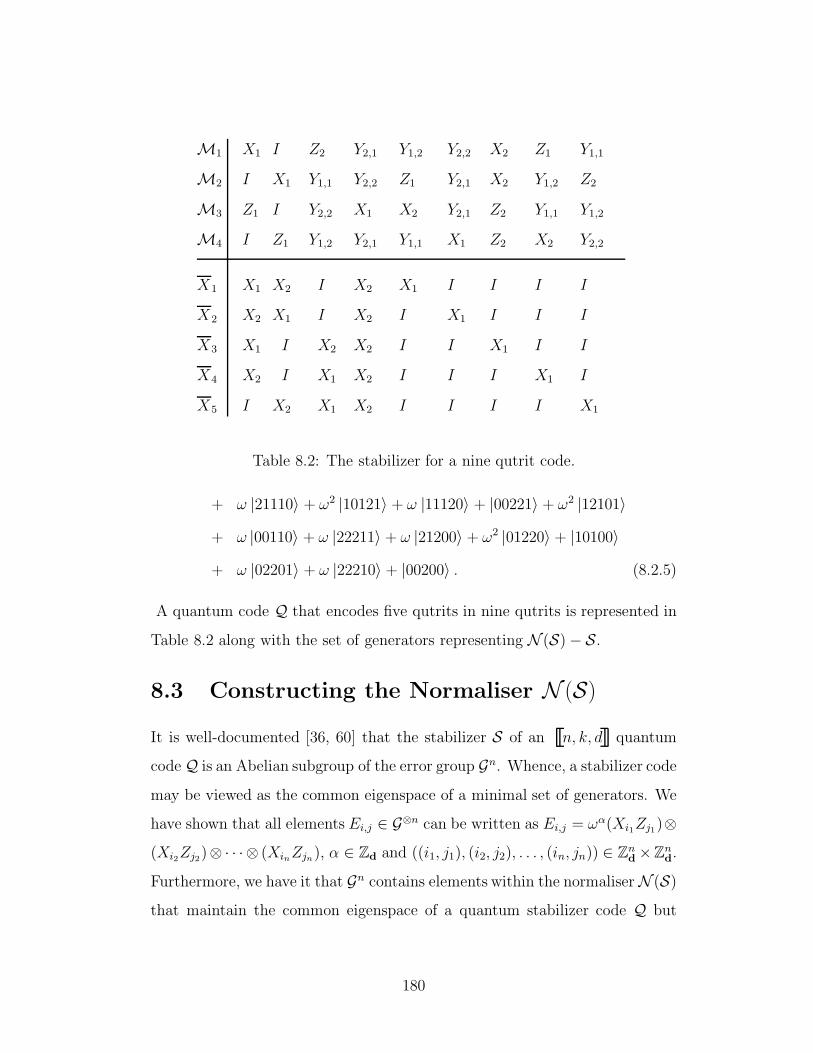
M1 X1 I Z2 Y2,1 Y1,2 Y2,2 X2 Z1 Y1,1
M2 I X1 Y1,1 Y2,2 Z1 Y2,1 X2 Y1,2 Z2
M3 Z1 I Y2,2 X1 X2 Y2,1 Z2 Y1,1 Y1,2
M4 I Z1 Y1,2 Y2,1 Y1,1 X1 Z2 X2 Y2,2
X1 X1 X2 I X2 X1 I I I I
X2 X2 X1 I X2 I X1 I I I
X3 X1 I X2 X2 I I X1 I I
X4 X2 I X1 X2 I I I X1 I
X5 I X2 X1 X2 I I I I X1
Table 8.2: The stabilizer for a nine qutrit code.
+ ω |21110〉 + ω2 |10121〉 + ω |11120〉 + |00221〉 + ω2 |12101〉
+ ω |00110〉 + ω |22211〉 + ω |21200〉 + ω2 |01220〉 + |10100〉
+ ω |02201〉 + ω |22210〉 + |00200〉 . (8.2.5)
A quantum code Q that encodes five qutrits in nine qutrits is represented in
Table 8.2 along with the set of generators representing N (S)− S.
8.3 Constructing the Normaliser N (S)
It is well-documented [36, 60] that the stabilizer S of an n, k, d quantum
codeQ is an Abelian subgroup of the error group Gn. Whence, a stabilizer code
may be viewed as the common eigenspace of a minimal set of generators. We
have shown that all elements Ei,j ∈ G⊗n can be written as Ei,j = ωα(Xi1Zj1)⊗
(Xi2Zj2)⊗ · · · ⊗ (XinZjn), α ∈ Zd and ((i1, j1), (i2, j2), . . . , (in, jn)) ∈ Znd×Zn
d.
Furthermore, we have it that Gn contains elements within the normaliserN (S)
that maintain the common eigenspace of a quantum stabilizer code Q but
180

which are not elements of the stabilizer S. This is a troublesome fact for a
coding theorist since codewords may be corrupted by errors that lie within
N (S). Such corruption cannot be corrected or detected but instead is past on
under the guise of some other codeword. The encoded information is lost and
the coding theorist is caught unawares and unknowing.
While elements ofN (S)− S act non-trivially within the common eigenspace
of the coding space C(S), N (S)− S permits the full description of the set of
quantum codewords. The 2k elements of N (S)− S are described by the sets
Xi and Zi where i = 1, . . . , k; see section 4.5. Lifting an n, k, dd
quan-
tum code to higher dimensions requires that the set N (S)− S be determined
according to conditions;
1. X i and Zj form independent and commuting sets that commute with
with eachM ∈ S.
2. X i commutes with Zj for i 6= j.
3. X i does not commute with Zj for i = j.
The following theorem determines commutativity between basis elements of
Cd which is then extended to the n-qudit setting.
Theorem 26. The operators Ei,j and Ek,l commute if and only if∑n
z=1 (jzkz − izlz)
vanishes.
Proof: Commutativity between the error operators Ei,j and Ek,l is estab-
lished following conjugation of Ei,j with Ek,l. In particular, we have it that
(XizZjz ) (XkzZlz) (XizZjz )−1
= (d−1∑
x=0
ωjzx |x+ iz〉 〈x|)(d−1∑
y=0
ωlzy |y + kz〉 〈y|)(d−1∑
z=0
ωjzz |z + iz〉 〈z|)−1
181

=d−1∑
x=0
ωjzx |x+ iz〉 〈x|d−1∑
y=0
ωlzy |y + kz〉 〈y|d−1∑
z=0
ω−jzz |z〉 〈z + iz|
=d−1∑
x=0
ωjzx |x+ iz〉 〈x|d−1∑
y,z=0
ωlzyω−jzz |y + kz〉 〈y|z〉 〈z + iz|
=
d−1∑
x=0
ωjzx |x+ iz〉 〈x|d−1∑
y=0
ωlzy−jzy |y + kz〉 〈y + iz|
=d−1∑
x,y=0
ωjzx+(lz−jz)y |x+ iz〉 〈x|y + kz〉 〈y + iz|
=d−1∑
y=0
ωjz(y+kx)+(lz−jz)y |y + kz + iz〉 〈y + iz|
=d−1∑
y=0
ωjzkz+lzy |y + kz + iz〉 〈y + iz|
=d−1∑
y=0
ωjzkz+lz(y−iz) |y + kz〉 〈y|
= ωjzkz−izlz
d−1∑
y=0
ωlzy |y + kz〉 〈y|
= ωjzkz−izlzXkzZlz . (8.3.1)
Hence Ei,jEk,lE−1i,j = ⊗n
z=1ωjzkz−iz lzXkzZlz . Consequently, Ei,j commutes with
Ek,l over Cdnif and only if
∑nz=1 (jzkz − izlz) vanishes.
The general form of the setX i is given by (β3i, β2i, β1i | α3i, α2i, α1i)T ∈ Z2n
d
where α1 and β1 are r-dimensional vectors, α2 and β2 are n−k−r-dimensional
vectors, and α3 and β3 are k-dimensional vectors. Correspondingly Zj has the
general form (β ′3i, β′
2i, β′
1i| α′
3i, α′
2i, α′
1i)T . To establish the 2k operators of
N (S) −S, we take the standard form of S and the general forms of X i and
Zj , and together with the conditions on N (S)− S over Cdn, we have it that
182

the set X i is determined by
βT1 +A2β
T3 −B5α
T3 = 0
−αT2 − C5α
T3 = 0
α3βT3 − αT
3 β3 = 0 (8.3.2)
while the set Zj is given by
β ′T1 +A2β
′T3 −B5α
′T3 = 0
−α′T2 −C5α
′T3 = 0 (8.3.3)
and the condition that X i does not commute with Zj imposes the further
requirement that
α′3β
T3 − αT
3 β′3 6= 0. (8.3.4)
Let us suppose that αT3 = 1 therefore α3 = 1, hence, α2 = −CT
5 . By Theorem
26 and constraint (8.3.2), we have α1 = β2 = 0. If we allow α′3 = β3 = 0 then
β ′3 = 1 and β ′
1 = −AT2 . Consequently, we have β1 = B5. Whence, the set
N (S)−S consisting of encoded X i and Zj vectors in a qudit quantum system
is given by
X =
00BT
5
−−I−CT
5
0
Z =
I0−AT
2
−−000
. (8.3.5)
8.4 Encoding a Qudit Stabilizer Code
Channel encoding permits the transmission of information through a quantum
system by embedding a (Cd)⊗k subspace within a (Cd)⊗n quantum system.
183

Cleve and Gottesman [19, 21] introduced an efficient scheme to compute the
encoding network for any qubit stabilizer code. For an n-qudit quantum code
defined by a set of n − k stabilizer elements, an encoding network transforms
a k-qudit information set into an n-qudit codeword. The basis states for
the coding space are obtained by implementing Gaussian elimination on the
n − k stabilizer set and appending the subsequent stabilizer set with a set
of logical-X operators. Finally, a set of Fourier operators is targeted on the
redundant elements of the encoding to ensure that the information content of
the codewords is defined by the (Cd)⊗k subspace. The requirement of orthog-
onality among codewords implies that the embedding is necessarily a unitary
transformation. Therefore, a decoding network can be implemented following
error-correcting techniques by reversing the order of the encoding transforma-
tion and applying the set of inverse gates that correspond to those gates of
the set of controlled operations. Table 8.3 illustrates an encoding scheme for
a qudit quantum code. A justification for the algorithm follows Table 8.3.
184

Table 8.3: Algorithm to compute an encoding network for a quditcode.
Input: Standard form of a code stabilizer, S.
Output: Encoding network for a qudit code.
1. A ← ∅
2. for b from 1 to (n− k)− 1 do
3. for a from b+ 1 to (n− k) do
4. Ma,b := Sa,b × Sb,b−1
5. for c from (n− k) + 1 to 2n do
6. Sa,c ← Sa,c −Ma,b × Sb,c
7. end
8. for d from b+ 1 to (n− k) do
9. Sa,d ← Sa,d −Ma,b × Sb,d
10. end
11. end
12. end
13. for a′ from 2 to (n− k) do
14. for b′ from a′ − 1 downto 1 do
185

15. Mb′,a′ := Sb′,a′ × Sa′,a′−1
16. for c′ from (n− k) + 1 to 2n do
17. Sb′,c′ ← Sb′,c′ −Mb′,a′ × Sa′,c′
18. end
19. for d′ from a′ + 1 to (n − k) do
20. Sb′,d′ ← Sb′,d′ −Mb′ ,a′ × Sa′,d′
21. end
22. end
23. end
24. r := rank of S
25. for b from n+ r + 1 to 2n− k − 1 do
26. for a from b− n + 1 to (n− k) do
27. Ma,b := Sa,b × Sb−n,b−1
28. for c from n+ r + 2 to 2n do
29. Sa,c ← Sa,c −Ma,b × Sb−n,c
30. end
31. for d from n+ 1 to n+ r do
32. Sa,d ← Sa,d −Ma,b × Sb−n,d
33. end
186

34. end
35. end
36. for b′ from n+ r + 2 to 2n− k do
37. for a′ from r + 1 to b′ − n− 1 do
38. Ma′,b′ := Sa′,b′ × Sb′−n,b′−1
39. for c′ from b′ + 1 to 2n do
40. Sa′,c′ ← Sa′,c′ −Ma′,b′ × Sa′+1,c′
41. end
42. for d′ from n+ 1 to n+ r do
43. Sa′,d′ ← Sa′ ,d′ −Ma′,b′ × Sa′+1,d′
44. end
45. end
46. end
47. for a from 1 to (n− k)
48. for b from 1 to 2n do
49. Sa,b ← S2n−b+1,(n−k)−a+1
50. end
51. end
52. for a′ from 2n downto n+ 1 do
187

53. find the first column l /∈ A where Sa′,l = 1
54. include l into A
55. end
56. for a from 1 to n do
57. for b from 1 to (n− k) do
58. Sa,b ← Sa,b × Sn+a,b
59. end
60. end
61. Append k columns of X to Sa,b
62. F ← ⊗l∈AF(l)
63. return (F,X,S).
We show the correctness of our algorithm. We can always perform Gaussian
elimination on S, the n−k×2n stabilizer matrix, without changing the system
it represents. This corresponds to Table 8.3 steps 2− 12. Let us assume that
the X matrix, the first n− k × n submatrix of S, has rank r ≤ n− k, then S
has the following form,(A | B0 | C
)(8.4.1)
whereA is an (r×n) submatrix of X. The Z submatrix of S takes no particular
form. We continue the algorithm by iterating on a′ over steps 13 − 23. This
allows us to obtain A in row-echleon form,(I A1 | B0 0 | C
)(8.4.2)
188

tt
tt
t
Z1
Z1F
F
F
F
Z1
Z2
Z1
Z2
Z1
X2
Z2
Z2
Z1
Z2
Z1
Z2
Z1input{
codeword
0
0
0
0
c1
Figure 8.2: Encoding circuit for a five qutrit code.
As the rows are linearly independent, C must have rank n − k − r, hence it
contains an (n− k − r× n− k − r) submatrix C2 of maximal rank. Thus, we
may produce a matrix whose form is given by,(I A1 A2 | B1 B2 B3
0 0 0 | C1 C2 C3
)(8.4.3)
In a similar manner to the row operations targeted on X, we begin another
stage of iteration on the submatrix C2. The algorithm steps 25 − 46 mirror
those of steps 2−23, and returns the submatrix C2 in row-echleon form. Steps
25 − 46 also act on the submatrices C1 and C3, transforming them to C4 and
C5 respectively. Given C2 = I, we may reduce B2 to the all zero matrix.
Further to this, submatrices C4 and C5 condition themselves on B1 and B3
respectively. The resulting stabilizer matrix is(I A1 A2 | B4 0 B5
0 0 0 | C4 I C5
)(8.4.4)
Steps 47 − 51 transpose the stabilizer and reverse the subsequent order of
columns. Algorithm steps 52 − 55 search for any columns l /∈ A such that
189

Sa′ ,l = 1, and updates A. The X and Z portions of the stylised S are amal-
gamated in steps 56− 60, before finally appending the encoded X ,
I−CT
5
BT5
, (8.4.5)
and Fourier set ⊗l∈AF(l) to S.
8.5 Correcting Procedure
The stabilizer formalism is well suited to meet the requirements of quantum
coding theory since it provides a compact basis to characterise the errors that
a code can detect and correct. This is qualified since the n − k stabilizers
M1,M2, . . . ,Mn−k can be seen to act as check operators for the code. Al-
ternatively, the stabilizer forms a set of collective observables that provide
non-demolition measurements which are used in the diagnosis of errors. The
set of non-demolition measurements is also known as the error syndrome for
the code. We consider a more formal approach to the calculation of the error
syndrome.
For stabilizer generators Mα and errors Eβ, we have
EβMαE−1β |ψ〉 = ςαβMα |ψ〉 (8.5.1)
for all |ψ〉 ∈ C. The set ςαβ, for α = 1, . . . , n−k, constitutes the error syndrome
for Eβ since ςαβ is the eigenvalue of Mα obtained by measuring Mα against
Eβ. In particular, we have it that ςαβ = ωnz=1 jzkz−iz lz. Recall that the error
correcting condition (2.3.2) for errors Eβ, Eβ′ ∈ En is given by
〈ψ|E−1β′ Eβ |ψ〉 = cβ′β. (8.5.2)
190

This condition is satisfied provided that one of the following holds
1. E−1β′ Eβ ∈ S
2. There exists some Mα ∈ S such that Mα does not commute with
E−1β′ Eβ.
Proof. Suppose E−1β′ Eβ ∈ S then 〈ψ|E−1
β′ Eβ |ψ〉 = 〈ψ|ψ〉 = 1. Next, suppose
that there is someMα ∈ S that does not commute with E−1β′ Eβ. Therefore,
(E−1β′ Eβ)Mα(E−1
β′ Eβ)−1
= ωnz=1 jz(kz−k′
z)−iz(lz−l′z)Mα (8.5.3)
with∑n
z=1 jz(kz − k′z)− iz(lz − l′z) 6= 0. Then
〈ψ|E−1β′ Eβ |ψ〉 = 〈ψ|E−1
β′ EβMα |ψ〉
= ωnz=1 jz(kz−k′
z)−iz(lz−l′z) 〈ψ|MiE−1β′ Eβ |ψ〉
= ωnz=1 jz(kz−k′
z)−iz(lz−l′z) 〈ψ|E−1β′ Eβ |ψ〉 (8.5.4)
is maintained when 〈ψ|E−1β′ Eβ |ψ〉 = 0. Thus, Eβ, Eβ′ form a set of correctable
errors for the stabilizer code C.
Should an error Eβ occur on the coding space C having an associated error
syndrome ςαβ = ωnz=1 jz(kz−k′
z)−iz(lz−l′z) for α = 1, . . . , n − k, then recovery is
achieved by applying E−1β = E−β. A quantum code is called nondegenerate if
there is a 1-1 correspondence between errors Eβ and syndrome ςαβ, otherwise,
the code is said to be degenerate. In the case of a degenerate code, there are
syndromes ςαβ and ςαβ′ for which ςαβ = ςαβ′ where Eβ 6= Eβ′. Correction will
induce a nontrivial action on the coding space C by mistakingly applying E−1β′
on a corrupted state of E−1β .
191
8.6 Complexity of a Qudit Stabilizer Code
Complexity measures the degree of efficiency to which an information pre-
serving function can be solved. We consider the computational complexity
of some problem function where focus is placed on the growth of a solution
time required against the size of the problem, and whose aim is to furnish an
appropriate result abstracted away from any particular circuitry architecture
simulating the function.
Consider the set of Boolean functions in LBk,n that describe the set of
all linear transformation from Fkq to Fn
q . The gate complexity of a function
f ∈ LBk,n, given by f(x) = Ax, is denoted C(A). In such case, A is a k × n
matrix with entries in Fq, and x = (x1, . . . , xn)t is a vector with elements in
Fq. The complexity of computing a Boolean function can be formalised by
the number of CNOT gates a circuit possesses. Consequently, C(A) is then
defined as the minimum number of CNOT gates needed to realise f . This
number is also referred to as the gate complexity of A. Byrne et al. [16]
determined the CNOT gate complexity of Hk, where Hk is the parity-check
matrix of the [2k−1, 2k−k−1] Hamming code. Furthermore, a general upper
bound on the complexity of functions in LBn,n has also been determined from
the complexity of the transpose of Hk [16].
Quantum computation is realised by a set of unitary operators that exhibit
a reversible nature. Thus, to illustrate equivalence between quantum compu-
tation and the Boolean function f , we require that f be a reversible function.
Therefore, recall the reversible function f given by f : Fdn+k 7→ Fd
n+k where
f (α; 0(n)) = (α; f(α)). Then, the computation of f corresponds to a unitary
operator Uf : Cdn+k 7→ Cdn+kin a quantum system. As a consequence, we
have the following result.
192

F
F
F
tt
tt
t Y1,1 Y2,1 Y1,2
X1 Y1,2 Y2,2
Z2 Y2,2 X2
X2 X2 Z1
Y2,2 Y1,1 Y1,1
X2 X2 X2 X2 Y2,1 Z2 Y2,1X2
Z2 Z1 Z2 Z2Z1Z2
Z1 Z2 Z1Z2
Z2 Z1 Z1 Z1 tt
t0
0
0
0
c5
c4
c3
c2
c1
input
codeword
Figure 8.3: Encoding circuit for a nine qutrit code.
Theorem 27. An upper bound on the complexity associated with the imple-
mentation of a qudit stabilizer code is 2n2/ log2 n.
Proof A qudit stabilizer code has an encoding circuit network of depth
n and width n which consists of CNOT and Phase gates. Byrne et al. [16]
have shown that 2n2/ log2 n is an upper bound on the gate complexity of
functions in LBn,n. As a consequence of quantum parallelism, the complexity
associated with implementing a stabilizer encoding is an instance of the CNOT
complexity of computing a function f in LBn,n, and the result follows.
193

M1 X1 Z1 Zd−1 Xd−1 I
M2 I X1 Z1 Zd−1 Xd−1
M3 Xd−1 I X1 Z1 Zd−1
M4 Zd−1 Xd−1 I X1 Z1
X1 Z1 I I Z1 X1
Z1 Z1 Z1 Z1 Z1 Z1
Table 8.4: The stabilizer for a five qudit code derived from the five qubit code.
194

Appendix
MAPLE PROGRAM: EXAMPLES
Calculate the roots αj, the coefficients βj and test the sequence aj =∑j/d
i=0
(j−(d−1)i
i
)
against the closed form∑d
l=1 βlαjl .
> restart;
Example 1. Test the closed form for the sum∑j/4
i=0
(j−3i
i
). The associated
generating function is 1− z− z4. The reciprocals of the roots of 1− z− z4 are
obtained from
> factor(z4 − z3 − 1, complex);
(z+.8191725134)(z−.2194474721+.9144736630I)(z−.2194474721−.9144736630I)(z−
1.380277569)
We calculate the values of the beta coefficients. As βl = −αl
B′(1/αl), we determine
each beta coefficient to be
> β1 = −(−.8191725134)/(−1 − 4 ∗ (1/(−.8191725134))3);
β1 = .1305102698
> β2 = −(.2194474721−.9144736630I)/(−1−4∗(1/(.2194474721−.9144736630I))3);
β2 = .1610008758 + .1534011260I
> β3 = −(.2194474721+.9144736630I)/(−1−4∗(1/(.2194474721+.9144736630I))3);
β3 = .1610008758 − .1534011260I
> β4 = −(1.380277569)/(−1 − 4 ∗ (1/(1.380277569))3);
β4 = .5474879784
We put the values of αl and βl from above into the closed form expression
∑dl=1 βlα
jl and generate instances of this expression.
> f := proc (j) options operator, arrow; (.1305102698) ∗ (−.8191725134)j +
195
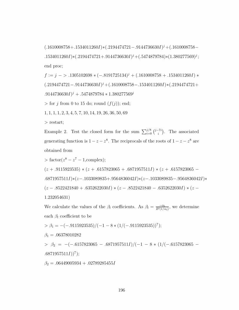
(.1610008758+.1534011260I)∗(.2194474721−.9144736630I)j +(.1610008758−
.1534011260I)∗(.2194474721+.9144736630I)j +(.5474879784)∗(1.380277569)j ;
end proc;
f := j − > .1305102698 ∗ (−.8191725134)j + (.1610008758 + .1534011260I) ∗
(.2194474721−.9144736630I)j +(.1610008758−.1534011260I)∗(.2194474721+
.9144736630I)j + .5474879784 ∗ 1.380277569j
> for j from 0 to 15 do; round (f(j)); end;
1, 1, 1, 1, 2, 3, 4, 5, 7, 10, 14, 19, 26, 36, 50, 69
> restart;
Example 2. Test the closed form for the sum∑j/8
i=0
(j−7i
i
). The associated
generating function is 1− z− z8. The reciprocals of the roots of 1− z− z8 are
obtained from
> factor(z8 − z7 − 1,complex);
(z + .9115923535) ∗ (z + .6157823065 + .6871957511I) ∗ (z + .6157823065 −
.6871957511I)∗(z−.1033089835+.9564836042I)∗(z−.1033089835−.9564836042I)∗
(z − .8522421840 + .6352622030I) ∗ (z − .8522421840 − .6352622030I) ∗ (z −
1.232054631)
We calculate the values of the βl coefficients. As βl = −αl
B′(1/αl), we determine
each βl coefficient to be
> β1 = −(−.9115923535)/(−1 − 8 ∗ (1/(−.9115923535))7);
β1 = .06378010282
> β2 = −(−.6157823065 − .6871957511I)/(−1 − 8 ∗ (1/(−.6157823065 −
.6871957511I))7);
β2 = .06449005934 + .02789285455I
196

> β3 = −(−.6157823065 + .6871957511I)/(−1 − 8 ∗ (1/(−.6157823065 +
.6871957511I))7);
β3 = .06449005934 − .02789285455I
> β4 = −(.1033089835−.9564836042I)/(−1−8∗(1/(.1033089835−.9564836042I))7);
β4 = .06911712233 + .06926484155I
> β5 = −(.1033089835+.9564836042I)/(−1−8∗(1/(.1033089835+.9564836042I))7);
β5 = .06911712233 − .06926484155I
> β6 = −(.8522421840−.6352622030I)/(−1−8∗(1/(.8522421840−.6352622030I))7);
β6 = .1188399306 + .1719523210I
> β7 = −(.8522421840+.6352622030I)/(−1−8∗(1/(.8522421840+.6352622030I))7);
β7 = .1188399306 − .1719523210I
> β8 = −(1.232054631)/(−1 − 8 ∗ (1/(1.232054631))7);
β8 = .4313256714
Put the values of αl and βl from above into the closed form expression∑d
l=1 βlαjl
and generate instances of this form.
> f := proc (j) options operator, arrow; (.06378010282) ∗ (−.9115923535)j +
(.0644+.0278I)∗(−.61578230−.68719575I)j +(.0644−.0278I)∗(−.61578230+
.68719575I)j +(.0691+ .0692I)∗(.10330898− .95648360I)j +(.0691− .0692I)∗
(.10330898 + .95648360I)j + (.1188 + .1719I) ∗ (.85224218 − .63526220I)j +
(.1188− .1719I) ∗ (.85224218+ .63526220I)j +(.4313256714) ∗ (1.232054631)j ;
end proc;
f := j − > .06378010282∗(−.9115923535)j +(.0644+ .0278I)∗(−.61578230−
.68719575I)j +(.0644−.0278I)∗(−.61578230+.68719575I)j +(.0691+.0692I)∗
(.10330898 − .95648360I)j + (.0691 − .0692I) ∗ (.10330898 + .95648360I)j +
197

(.1188 + .1719I) ∗ (.85224218− .63526220I)j +(.1188− .1719I) ∗ (.85224218 +
.63526220I)j + .4313256714 ∗ (1.232054631)j
> for j from 0 to 25 do; > round(f(j)); > end;
1, 1, 1, 1, 1, 1, 1, 1, 2, 3, 4, 5, 6, 7, 8, 9, 11, 14, 18, 23, 29, 36, 44, 53, 64, 78
198
Bibliography
[1] Aspect A, Dalibard J, and Roger G, Experimental Test of Bell’s Inequal-
ities Using Time-Verying Analyzers, Physical Review Letters, Vol. 49,
1982, pp. 1804-1807.
[2] Ashikhmin A, and Knill E, Nonbinary Quantum Stabilizer Codes, IEEE
Trans. Inform. Theory, Vol. 47, 2001, pp. 3065-3072.
[3] Barenco A, Bennett C H, Cleve R, DiVincenzo D P, Margolus N, Shor P,
Sleator T, Smolin J, and Weinfurter H, Elementary Gates for Quantum
Computation, Physical Review A, Vol. 52, 1995, pp. 3457-3488.
[4] Bell J, On the Einstein-Podolsky-Rosen Paradox, Physics, Vol. 1, 1964,
pp. 195-200.
[5] Bennett C H, Brassard G, Crepeau C, Jozsa R, Peres A, and Wooters A
K, Teleporting an Unknown Quantum State via Dual Classical and EPR
Channels, Physical Review Letters, Vol. 70, 1993, pp. 1895-1899.
[6] Bennett C H, Logical Reversibility of Computation, IBM J. Res. Develop.,
17, 525, 1973.
[7] Bergholm V, Vatiainen J J, Mottonen M, and Salomaa M M, Quantum
circuits with uniformly controlled one-qubit gates, Phys. Review A, 71,
052330, 2005.
199

[8] Bergholm V, Vatiainen J J, Mottonen M, and Salomaa M M, Quantum
circuits for general multiqubit gates, Phys. Review Letters, 93, 13, 2004.
[9] Blasiak, Horzela, Penson, Solomon, and Duchamp, Combinatorics and
Boson normal ordering: A gentle introduction, quant-ph/07043119, - ’A
very elegant way of storing and tackling information about sequences is
attained through their generating function.’
[10] Bose R C, and Ray-Choudhuri D K, On a class of error correcting binary
group codes, Information and Control, Vol. 3, 1960, pp. 68-79.
[11] Bouwmeester D, Ekert A, and Zeilinger A, The Physics of Quantum In-
formation, Springer, 2001, p. 163.
[12] Calderbank A R, Rains E M, Shor P W, and Sloane N J A, Quantum Error
Correction and Orthogonal Geometry, Physical Review Letters, Vol. 78,
1995, pp. 405-408.
[13] Calderbank A R, Rains E M, Shor P W, and Sloane N J A, Quantum
Error Correction via Codes over GF(4), IEEE Trans. Inform. Theory,
Vol. 44, 1998, pp. 1369-1387.
[14] Calderbank A R, and Shor P W, Good Quantum Error-Correcting Codes
exist, Physical Review A, Vol. 54, 1996, pp. 1098-1105.
[15] Cameron P J, Combinatorics: Topics, Techniques, Algorithms, Cam-
bridge University Press, 1994.
200

[16] Carmelo Interlando J, Byrne E, and Rosenthal J, The Gate Complexity
of Syndrome Decoding of Hamming Codes, Proceedings of the Tenth In-
ternational Conference on Applications of Computer Algebra, Beaumont,
Texas, 2004, pp. 33-37.
[17] Cirac J L, and Zoller P, Quantum Computations with Cold Trapped Ions,
Phys. Rev. Lett., Vol. 74, 1995, p. 4091-4094.
[18] Clarisse L, Ghosh S, Severini S, and Sudbery A, The disentangling power
of unitaries, quant-ph/0611075, 2006.
[19] Cleve R, and Gottesman D, Efficient computations of encodings for quan-
tum error correction, Phys. Rev. A, Vol. 56, 1997, pp. 76-82. LANL e-
print, quant-ph/9607030.
[20] Cleve R, Quantum Stabilizer Codes and Classical Linear Codes, Phys.
Rev. A, Vol. 55, 1997, pp. 4054-4059. LANL e-print, quant-ph/9612048.
[21] Cleve R, An Introduction to Quantum Complexity Theory, Collected Pa-
pers on Quantum Computation and Quantum Information Theory, eds.
C. Macchiavello, G.M. Palma, and A. Zeilinger, World Scientific, Singa-
pore, 2000. LANL e-print, quant-ph/9906111.
[22] Chuang I L, and Yamamoto Y, Quantum Bit Regeneration, Phys. Rev.
Letters, Vol. 76, 1996, pp. 4281-4284.
[23] Chuang I L, and Yamamoto Y, Creation of a persistent quantum bit using
error correction, Phys. Rev. A, Vol. 55, 1997, pp. 114-127.
201

[24] Deutsch D, Quantum theory, the Church-Turing principle and the univer-
sal quantum computer, Proc. Roy. Soc. Lond. A, Vol. 400, 1985, pp.97-117.
[25] Deutsch D, Quantum Computational Networks Proc. Roy. Soc. Lond. A,
Vol. 425, 1989, pp. 73-90.
[26] Deutsch D, Barenco A, and Ekert A, Universality in Quantum Computa-
tion, Proc. Roy. Soc. Lond. A, Vol. 449, 1995, pp. 669-677.
[27] DiVincenzo D P, Quantum Gates and Circuits, Proceedings of the ITP
Conference on Quantum Coherence and Decoherence, Proc. Roy. Soc.
Lond. A, Vol. 454, 1998, pp. 261-276. LANL e-print, quant-ph/9705009.
[28] Erdmann K, and Wildon M J, Introduction to Lie Algebras, Springer,
2006.
[29] Feynman R P, Simulating physics with computers. Int. J. Theor. Phys.
Vol. 21, 1982, pp. 467-488.
[30] Fowler A G, Dervitt S J, and Hollenberg L C L, Implementation of Shor’s
algorithm on a linear nearest neighbour qubit array, quant-ph/0402196,
2004.
[31] Gottesman D, A Class of Quantum Error-Correcting Codes saturating the
Quantum Hamming bound, Phys. Rev. A, Vol. 54, 1996, pp. 1862-1968.
[32] Gottesman D, Stabilizer Codes and Quantum Error Correction, Ph.D.
Thesis, Calif. Inst. Technol., Pasadena, CA, 1997.
202

[33] Gottesman D, Fault-Tolerant Quantum Computation with Higher-
Dimensional Systems, Quantum Computing and Quantum Communica-
tions, Proceedings of the 1st NASA International Conference on Quan-
tum Computing and Quantum Communications (QCQC), Palm Springs,
California, ed. C. Williams, New York, NY, Springer-Verlag, 1998, pp.
302-313. LANL e-print, quant-ph/9802007.
[34] Gottesman D, The Heisenberg Representation of Quantum Computers,
Group22: Proceedings of the XXII International Colloquium on Group
Theoretical Methods in Physics, eds. S. P. Corney, R. Delbourgo, and P.
D. Jarvis, Cambridge, MA, International Press, 1999, pp. 32-43. LANL
e-print, quant-ph/9807006.
[35] Graham R L, Knuth D E, and Patashnik O, Concrete Mathematics,
3rd ed., Addison-Wesley, 1994.
[36] Grassl M, Rotteler M, and Beth T, Efficient Quantum Circuits for Non-
Qubit Quantum Error-Correcting Codes, International Journal of Foun-
dations of Computer Science, Vol. 14, No. 5, 2003, pp. 757-775. LANL
e-print, quant-ph/0211014.
[37] Gershenfeld N, and Chuang I, Bulk Spin Resonance Quantum Computa-
tion, Science Vol. 275, 1997, pp.350-356.
[38] http://mathworld.wolfram.com/IrreducibleRepresentation.html.
[39] Hamming R W, Error Detecting and Error Correcting Codes, Bell System
Technical Journal, Vol. 26, 1950, pp. 147-160.
203

[40] Hardy Y, and Steeb W H, Decomposing the SWAP quantum gate, J. Phys.
A: Math. Gen. 39, 2006.
[41] Herstein I N, Topics in Algebra, 2nd ed., Wiley and Sons, 1975.
[42] Hill C D, Robust CNOT gates from almost any interaction, quant-
ph/0610059, 2006.
[43] Hocquenghem A, Codes correcteurs d’erreurs, Chiffres (Paris), Vol. 2,
1959, pp. 147-156.
[44] Hoffman D G, Leonard D A, Linder C C, Phelps K T, Rodger C A, Wall
J R, Coding Theory; The Essentials, Marcel Dekker, Inc., 1991, p. 38.
[45] Khaneja N, Brockett R, and Glaser S J, Time optimal control in spin
systems, Phys. Review A, 63, 032308, 2001.
[46] Klappenecker A, and Rotteler M, Unitary Error Bases: Constructions,
Equivalence and Applications, Lecture Notes in Computer Science, 2003,
2643, pages 139-149.
[47] Klappenecker A, and Rotteler M, Beyond Stabilizer Codes I: Nice Error
Bases, IEEE Trans. Inform. Theory, Vol. 48, 2002, pp. 2392-2395. LANL
e-print, quant-ph/0010082.
[48] Klappenecker A, and Rotteler M, Beyond Stabilizer Codes II: Clifford
Codes, IEEE Trans. Inform. Theory, Vol. 48, 2002, pp. 2396-2399. LANL
e-print, quant-ph/0010076.
204

[49] Klappenecker A, and Rotteler M, On the monomiality of nice error bases,
IEEE Trans. Inform. Theory, Vol. 51, 2005, pp. 1084-1089. LANL e-print,
quant-ph/0301078.
[50] Knill E, Group representations, error bases and quantum codes, Los
Alamos National Laboratory Report LAUR-96-2807, 1996.
[51] Knill E, Non-binary Unitary Error Bases and Quantum Codes, Los
Alamos National Laboratory Report LAUR-96-2717, 1996, quant-
ph/9608048.
[52] Knill E, and Laflamme R, A theory of quantum error-correcting codes,
Physical Review A, Vol. 55, No. 2, 1997, pp. 900-911.
[53] Liang L, and Li C, Realization of quantum SWAP gate between flying and
stationary qubits, Phys. Review A, 72, 024303, 2005.
[54] Lu F, and Marinescu D C, Quantum Error Correction of Time-Correlated
Errors, quant-ph/06052206.
[55] Lu C J, and Tsai S C, The Periodic Property of Binomial Coefficients
Modulo m and Its Applications, 10th SIAM Conference on Discrete Math-
ematics, Minneapolis, Minnesota, USA, 2000.
[56] http://www.maplesoft.com/
[57] MacWilliams F J, and Sloane N J A, The Theory of Error-Coreecting
Codes, North-Holland, Amsterdam, 1997.
205

[58] Monroe C, Meekhof D, King B, Itano W, and Wineland D, Demonstration
of a Fundamental Quantum Logic Gate, Phys. Rev. Lett., Vol 75, 1995,
pp. 4714-4717.
[59] Nielsen M A, A geometric approach to quantum circuit lower bounds,
quant-ph/0502070.
[60] Nielsen M A, and Chuang I L, Quantum Computations and Quantum
Information, Cambridge University Press, 2000.
[61] Nielsen M A, and Chuang I L, Quantum Computations and Quantum
Information, Cambridge University Press, 2000, p. 23.
[62] Nielsen M A, and Chuang I L, Quantum Computations and Quantum
Information, Cambridge University Press, 2000, p. 159.
[63] Nielsen M A, and Chuang I L, Quantum Computations and Quantum
Information, Cambridge University Press, 2000, p. 191.
[64] Nielsen M A, and Chuang I L, Quantum Computations and Quantum
Information, Cambridge University Press, 2000, p. 205.
[65] Nielsen M A, and Chuang I L, Quantum Computations and Quantum
Information, Cambridge University Press, 2000, p. 436.
[66] Nielsen A M, Knill E, and Laflamme R, Complete Quantum Teleportation
using Nuclear Magnetic Resonance, Nature, Vol. 396, No. 7706, 1998,
pp. 52-55.
206

[67] Petkovsek M, Wilf H, and Zeilberger D, A = B,
www.cis.upenn.edu/ wilf/AeqB.html.
[68] http://en.wikipedia.org/wiki/Separable polynomial.
[69] Plenio M B, and Knight P L, Realistic lower bounds for the factorisa-
tion time of large numbers on a quantum computer, Physical Review A,
Vol. 53, 1996, pp. 2986-2990.
[70] Preskill J, Quantum Computing: Pro and Con, Proc. Roy. Soc. Lond. A
Vol. 454, 1998, pp. 469-486. LANL e-print, quant-ph/9705032.
[71] Rains E M, Nonbinary quantum codes, IEEE Trans. Inform. Theory, Vol.
45, 1999, pp. 1827-1832.
[72] Rosen K H, Handbook of Discrete and Combinatorial Mathematics, CRC
Press, 2000.
[73] Schlingemann D, Problem 6 in open problems in Quantum Information
Theory, www.imaph.tu-bs.de/problems/
[74] Shannon C E, A Mathematical Theory of Communication, Bell System
Technical Journal, Vol. 27, 1995, pp. 379-423.
[75] Schumacher B, Quantum Coding, Phys. Rev. A, Vol. 51, 1995, pp. 2738-
2747.
[76] Sedlak M, and Plesch M, Towards optimization of quantum circuits,
quant-ph/0607123.
207
[77] Shende V, Markov I L, and Bullock S, Synthesis of Quantum Logic Cir-
cuits, IEEE Trans. on Computer-Aid Design, 25, no. 6, p. 100, 2006.
[78] Shende V, Markov I L, and Bullock S, Minimal universal two-qubit
controlled-NOT-based circuits, Phys. Review A, 69, 062321, 2004.
[79] Shor P W, Scheme for reducing decoherence in quantum computer mem-
ory, Physical Review A, Vol. 52, 1995, pp. 2493-2496.
[80] Shor P W, Polynomial-Time Algorithms for Prime Factorization and Dis-
crete Logarithms on a Quantum Computer, Proceedings of the 35th An-
nual Symposium on Foundations of Computer Science, 1994.
[81] Shor P W, and Laflamme R, Quantum Analog of the MacWilliams Identi-
ties for Classical Coding Theory, Phys. Rev. Lett., Vol. 78, 1997, pp. 1600-
1602.
[82] Steane A M, Quantum Reed-Muller Codes, IEEE Trans. Inform. Theory,
Vol. 45, No.5, 1999, pp. 1701-1703. LANL e-print, quant-ph/9608026.
[83] Steane A M, Multiple Particle Interference and Quantum Error Correc-
tion, Proc. Roy. Soc. Lond. A, Vol. 452, 1996, pp. 2551-2577. LANL
e-print, quant-ph/9601029.
[84] Steane A M, How to build a 300 bit, 1 Gop quantum computer, LANL
e-print, quant-ph/0412165.
208

[85] Testolin M J, Hill C D, Wellard C J, and Hollenberg L C L, A precise
CNOT gate in the presence of large fabrication induced variations of the
exchange interaction strength, e-print: quant-ph/0701165.
[86] Toffoli T, Reversible computing, Automata Languages and Programming,
Seventh Colloquium, Lecture Notes in Computer Science, Vol. 84, de
Bakker J W and van Leeuwen J, eds., Springer, 1985, pp. 632-644.
[87] Turchette Q, Hood C J, Lange W, Mabuchi H, and Kimble H J, Measure-
ment of Conditional phase Shifts for Quantum Logic, Phys. Rev. Lett.,
Vol. 75, 1995, pp. 4710-4713.
[88] Turing A M, On computable numbers, with an application to the Entschei-
dungsproblem, Proc. Lond. Math. Sco. 2, 42:230, 1936.
[89] http://en.wikipedia.org/wiki/Church-Turing thesis
[90] Vatan F, and Williams C, Optimal quantum circuits for general two-qubit
gates, Phys. Rev. A 69, 032315, 2004.
[91] Vidal G, and Dawson C M, Universal quantum circuit for two-qubit tran-
formations with three controlled-NOT gates, Phys. Rev. A 69, 2004.
[92] Vlasov A Y, Algebras and universal quantum computations with higher
dimensional systems, Proc. SPIE, Vol. 5128, 2003, pp. 29-36, LANL e-
print, quant-ph/0210049.
[93] Petkovsek M, Wilf H, and Zeilberger D, A=B,
http://www.math.upenn.edu/wilf/AeqB.html.
209

[94] Wilf H, generatingfunctionology, http://www.math.upenn.edu/wilf/gfology2.pdf.
[95] Werner R, All teleportation and dense coding schemes, J. Phys. A, vol.
34, pp. 7081-7094, 2001, quant-ph/0003070.
[96] Weyl H, The Thoery of Groups and Quantum Mechanics, Dover Publica-
tions, New York, 1931.
[97] Zanardi P, Zalka C, and Faoro L, Entangling power of quantum evolutions,
Phys. Review A, 62, 030301, 2000.
210


![Non-Stabilizer Quantum Codes from Abelian Subgroups of the Error … · 2018. 12. 17. · by Rains et al [RHSN97], all known quantum error-correcting codes are stabilizer codes. In](https://static.fdocuments.net/doc/165x107/60b9a7f715d91e53f713e924/non-stabilizer-quantum-codes-from-abelian-subgroups-of-the-error-2018-12-17.jpg)
![Quantum Codes from Classical Graphical Models · for the conversion of classical block codes to quantum codes. In [15], CPC code design was demonstrated using the ZX-calculus as well](https://static.fdocuments.net/doc/165x107/5fd86eb34b9c894a74223b66/quantum-codes-from-classical-graphical-models-for-the-conversion-of-classical-block.jpg)


