On Preprocessing the ALT-Algorithm - Fabian Fuchs · In dieser Studienarbeit wurde die...

On Preprocessing the ALT-Algorithm

Student Thesis of

Fabian Fuchs

At the faculty of Computer ScienceInstitute for Theoretical Informatics (ITI)

Reviewer: Prof. Dr. Dorothea WagnerAdvisor: Dipl.-Math. Reinhard BauerSecond advisor: Dr. Giacomo Nannicini

22. März 2010 – 12. Juli 2010

KIT – University of the State of Baden-Wuerttemberg and National Laboratory of the Helmholtz Association www.kit.edu

Ich versichere hiermit wahrheitsgemaß, die Arbeit bis auf die dem Aufgabensteller bereitsbekannte Hilfe selbstandig angefertigt, alle benutzten Hilfsmittel vollstandig und genauangegeben und alles kenntlich gemacht zu haben, was aus Arbeiten anderer unverandertoder mit Abanderung entnommen wurde.

Karlsruhe, den 12. Juli 2010. . . . . . . . . . . . . . . . . . . . . . . . . . . . . . . . . . . . . . . . . . . . . . . . . . . . . . . . . . . . . . . . . . . . . . . . . . . . . . . . . . . . . . . .Ort, Datum (Fabian Fuchs)

iv

Abstract

In this thesis, we study the preprocessing phase of the ALT algorithm. ALT is a wellknown preprocessing-based speed-up technique for Dijkstra’s algorithm, which allowsfast computations of shortest paths in large scale road networks. The preprocessingof the ALT algorithm has some degree of freedom, in that it must select a subset ofnodes in the graph, called landmarks, that fulfill a special role; optimally choosingthese landmarks is NP-hard, hence no effective exact solution algorithm exists. Inthis thesis, we study the landmark selection process; we propose several solutionmethods, including a greedy algorithm as well as a new heuristic. Furthermore, wepropose a new model for the search space of an ALT shortest path computation,which allows us to reduce the problem of optimally choosing k landmarks to themaximum coverage problem, for which approximation results are known, and toformulate the landmark selection problem as an integer linear program.

iv

v

Abstract

In dieser Studienarbeit wurde die Vorberechnungsphase des ALT Algorithmus’ un-tersucht. ALT ist ein bekannter und in der Literatur mehrfach untersuchter Routen-planungsalgorithmus der auf Dijkstra’s Algorithmus basiert aber durch einen Vor-berechnungsschritt kurzeste Wege Anfragen wesentlich schneller beantworten kann.Im Vorbereitungsschritt verbleiben gewisse Freiheitsgrade in der Wahl von speziellenPunkten, sogenannten Landmarken, zu und von denen die Entfernung zu allenanderen Knoten vorberechnet wird. Es ist NP hart diesen Freiheitsgrad optimalzu fullen, das heißt eine optimale Menge an Landmarken auszuwahlen, weshalbdafur bisher Heuristiken verwendet werden. In dieser Arbeit haben wir die Wahlder Landmarken untersucht und neue Losungsalgorithmen vorgestellt, darunter einGreedy Algorithmus sowie eine neue Heuristik. Des weiteren schlagen wir ein neuesSuchraummodel vor, das es uns ermoglicht das Problem auf ein ’Maximales Abdeck-ungsproblem’ (maximum coverage problem) zu reduzieren, fur das Approximation-sergebnisse existieren und das es uns ermoglicht das Problem der optimalen Wahlder Landmarken als Ganzzahliges Lineares Programm zu schreiben.

v

Contents

1 Introduction 1

2 Preliminaries 5

3 Landmarks 113.1 Search space model . . . . . . . . . . . . . . . . . . . . . . . . . . . . 113.2 Effect of landmarks on chains . . . . . . . . . . . . . . . . . . . . . . 143.3 Effect of landmarks on trees . . . . . . . . . . . . . . . . . . . . . . . 16

3.3.1 Potential πl+t (v) in undirected trees . . . . . . . . . . . . . . . 163.3.2 Potential πl−t (v) in undirected trees . . . . . . . . . . . . . . . 183.3.3 Undirected trees with combined potential πL

t () . . . . . . . . . 183.3.4 Optimal search spaces in trees . . . . . . . . . . . . . . . . . . 193.3.5 On paths between landmarks . . . . . . . . . . . . . . . . . . 21

4 Implementations and algorithms 254.1 Selecting landmarks as maximum coverage problem . . . . . . . . . . 254.2 Integer linear program . . . . . . . . . . . . . . . . . . . . . . . . . . 274.3 The greedy algorithm . . . . . . . . . . . . . . . . . . . . . . . . . . . 284.4 A new heuristic . . . . . . . . . . . . . . . . . . . . . . . . . . . . . . 304.5 The brute force algorithm . . . . . . . . . . . . . . . . . . . . . . . . 32

5 Experiments 335.1 Comparison with the Integer Linear Program . . . . . . . . . . . . . 345.2 Comparing the Greedy Algorithm . . . . . . . . . . . . . . . . . . . . 34

6 Conclusion 37

Bibliography 39

vii

1. Introduction

The computation of shortest paths on graphs is a problem with many real-life appli-cations like route planning in an internet or car navigation system, traffic simulationor logistic optimization. One prominent example is, that one is interested in theshortest path between two given endpoints: one departure node s and a destinationnode t. This variant of the problem, which is called the single-source single-targetproblem, can be solved in polynomial time with the well known Dijkstra’s algorithm(Dijkstra, 1959), assuming that the graph has non-negative edge weights. If thiscondition does not hold but the graph does not contain negative cycles, then theshortest path problem can be solved with the Bellman-Ford algorithm (Bellman,1958; Ford and Fulkerson, 1962). Finding a simple shortest path in graphs withnegative cycles is shown to be NP-hard. Indeed, these two algorithms can be usedto compute not only the shortest path between two given endpoints, but all shortestpaths originating from a source node s: this variant of the problem is called single-source. Although this is a very commonly used variant, there exist other variantsof the shortest path problem, such as the all-pairs shortest paths problem, whichrequires the computation of the shortest path between all pairs of nodes in a givengraph. The all-pairs shortest paths problem can be solved with the Floyd-Warshallalgorithm (Cormen et al., 2001).

One interesting practical application of the single-source single-target shortest pathproblem is route planning: indeed, road networks can be easily represented as graphs,and the problem of finding the shortest route between two points can be solved bycomputing the shortest path between two nodes on the corresponding graph. Inmany cases, one would be interested in computing shortest paths in a matter of fewmilliseconds: one typical example is a server scenario which has to deal with severaluser shortest paths queries per second, and is therefore required to carry out eachcomputation in a very short time. However, the graphs which represent real-worldroad networks, such as the European or the North American road networks, can havevery large sizes, and the classical shortest paths algorithms introduced above mayrequire several seconds for each computation. For the practical applications that wehave in mind, this is not acceptable. To deal with this issue, we can employ speed-uptechniques that preprocess the input data, in order to accelerate the answer to single-source single-target shortest paths queries (Wagner and Willhalm, 2007). This meansthat the solution method has two phases: a preprocessing phase, that computes

1

2 1. Introduction

u v

l1 l2

Figure 1.1: triangle inequality

useful information on the input graph and is applied only once, and a query phase,which computes the actual shortest paths using the output of the preprocessing phaseto accelerate the search. There are many different preprocessing based variantsof Dijkstra’s algorithm, such as ALT (Goldberg and Harrelson, 2004), Arc-Flags(Gutman, 2004), Contraction Hierarchies (Geisberger et al., 2008), Highway NodeRouting (Holzer et al., 2009; Schultes and Sanders, 2007), SHARC (Bauer andDelling, 2009) and Reach Based Pruning (Goldberg et al., 2007).

Research in this field is, at least for enhanced problems such as time-dependentgraphs, still very active, with the objective of improving preprocessing time andspace, as well as the performance of the query phase. An overview of several speed-up techniques and some experimental work can be found in (Delling et al., 2009;Wagner and Willhalm, 2007).

In this thesis we will take a closer look at the preprocessing phase required by theALT algorithm, which has been introduced by (Goldberg and Harrelson, 2004). ALTstands for A* search, Landmarks and Triangle inequality, as these are the mainingredients of the algorithm. The A* algorithm is a generalization of Dijkstra’salgorithm, which uses a function (the potential function π) to estimate distancesbetween nodes in the graph. A good potential function π can be used to reduce thesearch space (i.e. the set of nodes that have to be “explored” before the solution isfound) of the shortest path queries effectively. One way to define a potential functionis through the use of landmarks (Goldberg and Harrelson, 2004), that is, a subset ofthe nodes in the graph which fulfill a special role. For these landmarks, the distancesto/from all other nodes in the graph are computed during the preprocessing phase,and estimations of distances within the graph can then be carried out by means ofthe triangle inequality. The triangle inequality states that, for any three nodes u, v, lin the graph, d(u, v) ≤ d(u, l) + d(l, v), where d(u, v) is the distance between u andv, i.e. the length of the shortest path between those two nodes. This inequality canbe used to derive bounds: as illustrated in Figure 1.1, the distance from u to v issmaller than dist(l1, v) − dist(l1, u) as well as dist(u, l2) − dist(v, l2). One questionarises: how do we select landmarks on the input graph?

As it is shown in (Bauer et al., 2010), most of the preprocessing based speed-uptechniques for Dijkstra’s algorithm (such as ALT, Arc-Flags, SHARC, Highway NodeRouting and Contraction Hierarchies), have some degrees of freedom which are NP-hard to determine optimally, and are therefore heuristically determined in practice.This also applies for the ALT algorithm, for which it is shown that selecting aset of k landmarks which minimizes the expected search space for random single-source single-target queries is NP-hard. Several heuristics for this purpose havebeen proposed in the literature, such as: random, farthest and avoid introduced byGoldberg and Harrelson (Goldberg and Harrelson, 2004), advanced avoid introducedby Delling et al (Delling et al., 2006), as well as maxCover introduced by Goldbergand Werneck (Goldberg and Werneck, 2005).

2

3

In this thesis we will study the problem of selecting the set of landmarks in a graphso that the search space of random single-source single-target shortest path queriesis minimized. We will focus on simple graph classes such as paths and trees, andgive results on the effect that landmarks have on the shortest paths computations.We will also give an upper bound on the number of landmarks which are needed toachieve minimal search spaces in trees. We will then analyze the performance of agreedy algorithms for the problem of selecting k landmarks, and introduce a newheuristic. We propose an integer linear program (ILP) formulation that models theproblem of selecting the best possible set of landmarks on a given graph. Finally, wecarry out computational experiments to compare the performance of the methodsstudied in this thesis with existing algorithms from the literature.

3

2. Preliminaries

We denote by

N the set of non-negative integersR+ the set of positive real numbers, including zero|A| the cardinality of the set A

A graph is an ordered pair G = (V,E) comprising a set V of vertices and a set E ⊂ V×Vof edges. We also consider a non-negative length function len : E → R+; for the sake ofsimplicity, we write len(u, v) := len((u, v)).

Definition and Remark 2.1. For a graph G = (V,E)

1. G is said to be directed if the elements of E are ordered pairs, and is called undirectedif such pairs are unordered.

2. For a directed graph, we say that an edge e = (u, v) leaves node u and enters nodev.

3. Within this thesis, an undirected graph is equivalent to a directed graph such thatfor every edge e = (u, v) ∈ E there exists an edge e′ = (v, u) ∈ E.

4. For an undirected graph, the length function is required to be symmetric: len(u, v) =len(v, u).

Definition 2.2. Given a graph G = (V,E) and two nodes u, v ∈ V

1. A path from u to v (also called a u-v-path) is a sequence (v0, v1, . . . , vp) of vertices suchthat u = v0,v = vp, and there exists an edge (vi−1, vi) ∈ E for every i ∈ {1, . . . , p}.

2. A path from u to v is called simple if no vertices are repeated on the path.

3. The distance between two vertices u and v is defined as

dist(u, v) := min(v0,...,vp) is a path from u to v

p∑i=1

len(vi−1, vi).

and if no path from u to v exists in G, dist(u, v) :=∞ by convention.

4. Given u, s, t ∈ V, and an s-t-path Q, we define the distance between u and Q asdist(u,Q) := minv∈Q{dist(s, v)}.

5

6 2. Preliminaries

5. A cycle is a path (v0, v1, . . . , vr) with v0 = vr.

6. If we require the path (v0, v1, . . . , vr−1) to be simple we say (v0, v1, . . . , vr) is a simplecycle.

Definition and Remark 2.3. For a graph G = (V,E)

1. We say G is connected if for each pair (u, v) ∈ V ×V a path from u to v exists.

2. G is a tree if G is connected and without cycles.

3. In a tree any two vertices are connected by exactly one shortest path.

4. we call G a chain if for V = {v0, . . . , vn} the set of edges is E = {(v0, v1), (v1, v2), . . . , (vn−1, vn)},intuitively speaking the graph is one path.

Dijkstra’s Algorithm

Given a graph G = (V,E) with non-negative length function len(·, ·) and a source s anda target t with s, t ∈ V, Dijkstra’s algorithm computes the distances and shortest pathsfrom the source to the target.

During the run of the algorithm a vertex can have three different states: It is eitherunreached, reached or settled. It is unreached while the distance label is set to infinity,reached as soon as a tentative shortest path from the source to the vertex has been foundand settled once it has been processed by the algorithm (Step 1 and 2). Note that ashortest path from s to a vertex v has been found if v is settled. If v is reached, a tentativepath from s to v has been found which is not necessarily shortest.

The algorithm initializes a distance label dist(v) = ∞ for every vertex v ∈ V\{s} anddist(s) to 0. We use a min-based priority queue Q to manage the reached vertices priorizedby the distance label. Then, Step 1 and Step 2 are executed until the priority queue Q isempty which is equally to that every reachable vertex has been settled.

Step 1. Select the reached vertex v with smallest distance label dist(v). If there is morethan one with the same distance label there is some freedom left in how to break ties. Themost common way is to compare the vertex’s ID and select the vertex with the smallestID.Step 2. For every edge from v to a vertex u, update the distance label dist(u) if dist(v) +len(v, u) is smaller than the current distance label dist(u) to dist(u) = dist(v) + len(v, u).If the distance label is updated, the algorithm found a new tentative shortest path from sto the vertex u. Hence we update parent(u): parent(u) = v and add u to priority queueQ if it has not yet been added, i.e. if u has been unreached so far. Finally the state of thevertex v is changed to settled.

For every vertex v such that its state is settled, the distance from s to v is dist(s, v) =dist(v). If a vertex’s distance label is still set to infinity after the algorithm ended thisvertex can not be reached from s. The shortest path from s to a settled vertex v is encodedin the parent(·) label, which must be followed from v to s to decode the shortest path froms to v.

Definition 2.4. In a graph G = (V,E) with positive length function len(·, ·) we call theset of vertices which are settled during the run of Dijkstra’s algorithm for an s-t-query theDijkstra search space of this s-t-query and denote it by VDij(s, t).

A* search

6

7

Algorithm 2.1 Dijkstra(G, s, t)

Require: graph G = (V,E) and Vertices s, tVEnsure: dist(s, v) = dist(v)∀v ∈ V1: for all v ∈ V do2: parent(v)← ⊥3: state(v) ← unreached4: dist(v)←∞5: dist(s)← 06: state(s) ← reached7: while vertex v with state(v) = reached exists and state(t) 6= reached do8: Select v ∈ V with state(v) = reached and minimal dist(v)9: for all u ∈ V with (v, u) ∈ E do

10: if dist(v) + len(v, u) < dist(u) then11: dist(u)← dist(v) + len(v, u)12: parent(u)← v13: state(u) ← reached14: state(v) ← settled

For a given graph G = (V,E) with non-negative length function len(·, ·), a source s ∈ V,a target t ∈ V and a so called potential function πt : V → R+, A*-search computes thedistance from s to t. A* is a generalization of Dijkstra’s algorithm, which uses a potentialfunction πt in addition to the distance function to select the node which should be visitednext. The potential function πt(v) is usually a lower bound for the distance from anyvertex v to the target t.

The potential function πt has to be feasible: dist(u, v)− πt(u) + πt(v) ≥ 0 for all verticesu, v ∈ V. This implies that the resulting new edge ”lengths” len(u, v) := len(u, v)−πt(u)+πt(v) are still positive, which is necessary for Dijkstra’s algorithm as well as A* search towork correctly. With these new edge lengths Dijkstra is equal to A* search, which is provedin section 3.1.

A* works exactly as Dijkstra, except that the algorithm stops once the target is settledand that in Step 1 the reached vertex which has minimal costs cost(v) := dist(v) + πt(v)is selected. In general, we write cost(v) := dist(s, v) + πt(v) which is equal to cost(v) forall settled nodes v after the execution of A* search with source s.

ALT algorithm

The ALT algorithm is a variant of A* search, whose main idea is to use landmarks andtriangle inequality to compute a feasible potential function. Given a graph G = (V,E)with non-negative length function len(·, ·), ALT first selects a set L ⊂ V of k landmarksand precomputes the distance to and from these landmarks for every vertex in V duringa preprocessing step.

With the triangle inequality |x+y| ≤ |x|+|y| we can derive the two inequalities dist(u, v) ≥dist(l, v)−dist(l, u) and dist(u, v) ≥ dist(u, l)−dist(v, l) for any u, v, l ∈ V. Note that theright hand sides only involve distances to and from a landmark which we assumed to beavailable thanks to the preprocessing. With the convention ∞−∞ := 0, we can thereforedefine

πl+t (v) := dist(v, l)− dist(t, l) (2.1)

πl−t (v) := dist(l, t)− dist(l, v) (2.2)

7

8 2. Preliminaries

Algorithm 2.2 A*(G, s, t, πt)

Require: graph G = (V,E), Vertices s and tEnsure: parent(t) encodes the shortest path from s to t1: for all v ∈ V do2: parent(v)← ⊥3: state(v) ← unreached4: dist(v)←∞5: dist(s)← 06: state(s) ← reached7: while vertex v with state(v) = reached exists and state(t) 6= reached do8: Select v ∈ V with state(v) = reached and minimal cost(v) = dist(v) + πt(v)9: for all u ∈ V with (v, u) ∈ E do

10: if dist(v) + len(v, u) + πt(u) < dist(u) + πt(u) then11: parent(u)← v12: dist(u)← dist(v) + len(v, u)13: state(u) ← reached14: state(v) ← settled

as feasible potential functions. To get the tightest bounds we use the maximum of thesepotential functions for all landmarks and define

πLt (v) := maxl∈L{πl+t (v), πl−t (v)} (2.3)

as the potential function ALT uses for the A* search algorithm.

Definition 2.5. In a graph G = (V,E) with positive length function len(·, ·) we call theset of vertices which are settled during the run of ALT for an s-t-query the ALT searchspace of this s-t-query. Since the search space of an s-t-query of ALT depends on the setof landmarks, we denote the search space in the ALT algorithm by VL(s, t).

Note that we did not specify how to break ties when extracting nodes from the prioriryqueue Q, i.e. the case where multiple nodes attain the minimum on line 8 of Algorithm2.3. This can have an impact on the search space: see Section 3.1.

8

9

Algorithm 2.3 ALT(G, s, t)

Require: graph G = (V,E), Vertices s and tEnsure: parent(t) encodes the shortest path from s to t1: L = generate Landmarks(G, k) {select set of k landmark}2: for all v ∈ V do3: parent(v)← ⊥4: state(v) ← unreached5: dist(s, v)←∞6: dist(s, s)← 07: state(s) ← reached8: while vertex v with state(v) = reached exists and state(t) 6= reached do9: Select v ∈ V with state(v) = reached and minimal cost(v) = dist(s, v) + πLt (v)

10: for all u ∈ V with (v, u) ∈ E do11: if dist(s, v) + len(v, u) + πLt (u) < dist(s, u) + πLt (u) then12: parent(u)← v13: dist(s, u)← dist(s, v) + len(v, u)14: state(u) ← reached15: state(v) ← settled

9

3. Landmarks

The selection of good landmarks is a crucial point for the performance of the ALT algo-rithm. Since good landmarks yield a tight lower bound on the distance from any vertexto the target, with better landmarks usually fewer vertices must be settled by the ALTalgorithm. Therefore, the search space of these s-t-queries can be reduced.

In order to compare different sets of landmarks, we need a measure of quality. We decidedto use the sum of the sizes of the search spaces over all s-t-queries as a measure of qualityfor a given set of landmarks L: ∑

s,t∈VVL(s, t) (3.1)

Minimizing this quantity is equivalent to minimizing the average size of the search spacefor a random s-t-query. This results in the following minimization problem. Solving thisproblem and therefore minimizing the average size of the search space for a random s-t-query will be our objective in this thesis.

Definition 3.1 (MinALT). Given a graph G = (V,E) and an integer k, the problemMinALT is the problem of selecting k landmarks so that the resulting overall ALT searchspace is minimal, i.e.to select a set L ⊂ V so that

∑s,t∈V VL(s, t) is minimal.

3.1 Search space model

In order to measure the search space, we need a model we can compute without having torun the algorithm itself. Therefore, in literature, a search space model was first describedby (Bauer et al., 2010). It is motivated by the proof of Theorem 4.1 in (Goldberg andHarrelson, 2004).

Theorem (Goldberg 4.1 [incorrect]). Let πt and π′t be two feasible potential function suchthat πt(t) = π′t(t) = 0 and for any vertex π′t(v) ≥ πt(v) (i.e. π′t dominates πt). Thenthe set of vertices scanned by A* search search using π′t is a subset of the set of verticesscanned by A* search search using πt.

This is not true, since for example let G = (V,E) be a undirected graph with V ={0, 1, 2, 3, 4, 5} and E = {(0, 2), (0, 3), (1, 3), (1, 4), (1, 5), (2, 4), (2, 5), (3, 4), (3, 5)} with edgelengths 1 except for the edges (2, 4), (2, 5) and (3, 5) which have edge lengths 2. For sim-plicity every undirected edge is given only once. The graph is illustrated in Figure 3.1.

11

12 3. Landmarks

1

4

302

5

2

2

2

(a)

1

4

302

5

2

2

2

(b)

1

4

302

5

2

2

2

(c)

Figure 3.1: A counterexample to Theorem 4.1 in (Goldberg and Harrelson, 2004). On theleft the graph in which the counterexample can be constructed is shown. All edge lengthsare 1 if not stated otherwise. In the graph in the middle the ALT search space of the0-1-query using the landmark 4 is illustrated. On the right the same search space is shown

using the landmarks {4, 5}.

For a query from source vertex s = 0 to sink vertex t = 1, we will first examine the searchspace for the potential πLt induced by the landmark L = {4}.

In the first step of the ALT algorithm, the to the vertex 0 adjacent vertices 2 and 3 arereached. ˆcost(2) = dist(2)+πLt (2) = 1+1 = 2 whereas ˆcost(3) = dist(3)+πLt (3) = 1+0 = 1,hence 3 is settled next. Then, the target 1 is reached with ˆcost(1) = dist(1) + πLt (1) =2 + 0 = 2. There is a tie between vertices 1 and 2, but vertex 1 is settled since 1 < 2. Thesearch space is therefore {0, 3, 1}.

Using the potential πL′

t induced by the landmarks L′ = {4, 5} in the first step of the ALTalgorithm the costs for vertex 2 are the same but for vertex 3 they change to ˆcost(3) =dist(0, 3) + πL

′t (3) = 1 + 1 = 2. Since the costs are the same the tie is broken by settling

the one with the smaller ID. Hence 2 is settled first, then 3 will get settled and afterwardsthe target vertex 1. The resulting search space is {0, 2, 3, 1}.

One can easily check that the potential πL′

t dominates πLt since the maximum over thepotentials induced by the landmarks is taken as described in Chapter 2.

The search space deduced from the way Goldberg breaks ties, would be

VL(s, t) = {v ∈ V|dist(s, v) + πLt (v) < dist(s, t) or

dist(s, v) + πLt (v) = dist(s, t) and v ≤ t}(3.2)

for a s-t-query in a graph G = (V,E) with a set of landmarks L.

In contrast to VL(s, t), the search space model we will work with is the worst case searchspace model, which can be expressed as

VL(s, t) = {v ∈ V|dist(s, v) + πLt (v) ≤ dist(s, t)} (3.3)

If it is not clear which graph G is meant, we will write VL,G(s, t).

In the following theorem we show, that using the worst case search space model is reason-able.

Theorem 1. Let G = (V,E) be a graph, L a set of landmarks and the length function bestrictly positive: len(u, v) > 0 for any u, v ∈ V.Assuming ALT breaks ties based on the labeling of vertices, then there is a labeling of Gsuch that the ALT search space VL(s, t) equals VL(s, t).

12

3.1. Search space model 13

To show the theorem we first show that executing the ALT algorithm is equivalent toexecuting Dijkstra’s algorithm with altered length function. Then, we show that thetheorem holds for Dijkstra with altered length function.

Lemma. On a graph G = (V,E) with non-negative length function len(·, ·), executing A*search with the feasible potential π is equivalent to Dijkstra’s algorithm with altered lengthfunction len(u, v) := len(u, v) + π(v)− π(u).This means that the nodes are settled in the same order for both algorithms. We assumethat ties are broken in the same way for both algorithms.

Proof. During the initialization both algorithms do the same (state(v)=unreached, dist(v) =∞ / dist(v) =∞, for v ∈ V and dist(s) = dist(s) = 0).For both algorithms the loop executes as long as there are unsettled vertices and the targett is not settled.In the loop Dijkstra selects the vertex v with smallest distance label dist(v) whereas onthe other hand A* search selects the vertex v with smallest dist(v) + πt(v).We will prove by induction that both algorithms settle the nodes in the same orderwhich means that dist(v) and dist(v) + πt(v) are the same up to a constant factor c:dist(v) = dist(v) + πt(v)− πt(s) with c = −πt(s).

Base case: The first settled vertex is in both algorithms s and dist(s) = 0 = dist(s) +πt(s)− πt(s).

Let the first r vertices be settled in the same order by both algorithms and dist(v) =dist(v) + πt(v)− πt(s) for all vertices v.Induction step: Let v be the (r + 1)th vertex which is settled by Dijkstra’s algorithm.

Then dist(v)induction

= dist(v) + πt(v)− πt(s) must be minimal and hence dist(v) + πt(v) =dist(v)+πt(s) is minimal. In case there is a tie in both algorithms the same vertex is chosen,too. Then the distances are updated for any to v adjacent vertex u if dist(v) + len(v, u) <dist(u) in both algorithms. A* search updates the distance to dist(u) = dist(v) + len(u, v)and Dijkstra to dist(u) = dist(v) + len(v, u) = dist(v) + πt(v)− πt(s) + len(v, u) + πt(u)−πt(v) = dist(v) + len(v, u) + πt(u) − πt(s) = dist(u) + πt(u) − πt(s). And therefore bothalgorithms are settling the same r+ 1th vertex and dist(v) = dist(v) + πt(v)− πt(s) aftersettling the r + 1th vertex.

Since both algorithms end once the target is settled the lemma is shown.

Proof of Theorem 1. Given a graph G = (V,E) with L, πLt as in the theorem, len(u, v) :=len(u, v) + πLt (v) − πLt (u) the length function and vertices s, t ∈ V and an node labelingα : V→ N such that

α(v) 6= α(u) if v 6= u

α(t) > α(v) for all v ∈ V

We have to show that VGα

Dij(s, t) = VL,G(s, t).

”⊆”: Let therefore be s, t, v ∈ V such that v ∈ VGα

Dij(s, t), then:

case dist(s, v) ≤ dist(s, t): v ∈ VL,G(s, t) due to the definition of VL,G(s, t).

case dist(s, v) > dist(s, t): t is settled before v is settled and therefore v 6∈ VGα

Dij(s, t), i.e.this case is not possible.

”⊇”: Let s, t, v ∈ V such that v ∈ VL,G(s, t), then:

case dist(s, v) + πLt (v) < dist(s, t): Dijkstra settles all vertices with dist(s, v) + πLt (v) −πLt (s) < dist(s, t)− πLt (s) before t is settled ⇒ v ∈ VGα

Dij(s, t).

13

14 3. Landmarks

case dist(s, v) + πLt (v) = dist(s, t): For a path Q from s to v it holds for all vertices w ∈ Qthat dist(s, w)+πLt (w) ≤ dist(s, t). Hence it is sufficient to show that a path Q froms to v with vertices in the Dijkstra search space exists such that t 6∈ Q.We first show that t 6∈ Q: Assume t is on the path Q then dist(s, v) + πLt (v) =

dist(s, t) + dist(t, v) + πLt (v)dist(t,v)>0

> dist(s, t) and hence v is not in VL,G(s, t).Now we show that the (shortest) path from s to v (including v) is in the Dijkstrasearch space. We prove that by induction over the vertices s = w0, w1, . . . , wr = von the path Q.Base case: s = w0 is in the Dijkstra search space.Induction step: If dist(s, wi) + πLt (wi) < dist(s, t) the first case applies and hencewi ∈ VGα

Dij(s, t).

If dist(s, wi) + πLt (wi) = dist(s, t) all vertices wj with j < i are in the Dijkstrasearch space and hence the distance label of the vertex wi is dist(wi) = dist(s, wi).Since dist(s, wi) + πLt (wi) <= dist(s, t) there is a tie and Dijkstra settles wi sinceα(wi) < α(t).

Remark 3.2. From the theorem follows, that the search space of the ALT algorithm foran s-t-query can not generally (i.e. if the vertex labeling is unknown) be bound tighterthan {v ∈ V|dist(s, v) + πLt (v) ≤ dist(s, t)} using a total order function < comparing avertex’s ID to the target’s ID to break ties on a graph with strictly positive length function.

Now that we justified our new search space model VL(s, t), we show that the statementof theorem 4.1 from (Goldberg and Harrelson, 2004) is correct for our search space model.

Definition 3.3. On a graph G = (V,E) with positive length function, a set of landmarksL and feasible potential πLt we write VπL

t(s, t) if it is not clear which potential is meant.

Theorem 2. Let πt and π′t be two feasible potential function such that πt(t) = π′t(t) = 0and for any vertex π′t(v) ≥ πt(v) (i.e. π′t dominates πt). Then the set of vertices in thesearch space Vπ′

t(s, t) settled by ALT using π′t is a subset of the set of vertices in the search

space Vπt(s, t) settled by ALT using πt.

Proof. Suppose that a vertex v is not settled by ALT using the potential Vπt(s, t). It issufficient to show that v is not settled by ALT using the potential Vπ′

t(s, t). Since v is not

settled, it must be that dist(s, v) + πt(v) > dist(s, t). Since π′t dominates πt it holds thatdist(s, v) + π′t(v) ≥ dist(s, v) + πt(v) > dist(s, t) and hence v is not settled by ALT usingthe potential π′t(v).

3.2 Effect of landmarks on chains

In this section, we show the effect landmarks have on ALT queries on chain graphs.

Definition 3.4. The search space of a graph is optimal if the overall search space∑s,t∈V VL(s, t) is minimal, i.e. it can not be improved any further.

Theorem 3. Using only one landmark, a graph G consisting of only one chain of vertices(v0, v1, . . . , vn), n ≥ 3 with strictly positive length function len, has optimal search space,if and only if v0 or vn is a landmark

Proof. ”→”: Let G be a graph as in Theorem 3.

14

3.2. Effect of landmarks on chains 15

Assume that the landmark is L = {vj}, j 6= 0, j 6= n. Consider the query with sourcevj and the target be the to vj adjacent vertex to which the connecting edge has a higherlength. W.l.o.g this be vj+1. Then the costs of vj−1 and vj+1 are

cost(vj−1) = dist(vj , vj−1) + πLvj+1(vj−1)

= dist(vj , vj−1) + max{dist(vj−1, vj)− dist(vj+1, vj),dist(vj+1, vj)− dist(vj−1, vj)}= dist(vj , vj−1) + dist(vj+1, vj)− dist(vj−1, vj)

= dist(vj+1, vj)

and

cost(vj+1) = dist(vj , vj+1) + πLvj+1(vj+1)

= dist(vj , vj+1) + max{dist(vj+1, vj)− dist(vj+1, vj),dist(vj+1, vj)− dist(vj+1, vj)}= dist(vj , vj+1)

and therefore both are in VL(s, t) and the query is not optimal.

”←”:

Let G be such a graph and w.l.o.g. v0 be the landmark (otherwise relabel the chain). Weshow that all s-t-queries have a minimal search space.

Let therefore s, t ∈ V be two vertices such that the search space of the s-t query is notminimal without using landmarks, i.e. VDij(s, t) 6= (s = u0, u1, . . . , ur = t). It is shownin → that such a query exists (e.g. from the source v1 to its adjacent vertex with highercosts).

We know that without using landmarks at least the one vertex adjacent to the source whichis not on the s-t-path must be settled (otherwise the query would be optimal, since behindthe target no vertex is in the search space due to the strictly positive length function).Let the source be s = vi and the target t = vl then either vi+1 or vi−1 is in the Dijkstrasearch space but not on the s-t-path. In the first case l < i and in the latter l > i. In thefirst case the costs for vi+1 are

cost(vi+1) = dist(vi, vi+1) + πt(vi+1)

= dist(vi, vi+1) + max{dist(vi+1, v0)− dist(t, v0), dist(v0, t)− dist(v0, vi+1)}= dist(vi, vi+1) + dist(vi+1, v0)− dist(t, v0)

= dist(vi, vi+1) + dist(vi+1, t)

= dist(vi, t) + 2 dist(vi, vi+1)

= dist(s, t) + 2 dist(vi, vi+1)

and in the latter case the costs for vi−1 are

cost(vi−1) = dist(vi, vi−1) + πt(vi−1)

= dist(vi, vi−1) + max{dist(vi−1, v0)− dist(t, v0), dist(v0, t)− dist(v0, vi−1)}= dist(vi, vi−1) + dist(v0, t)− dist(v0, vi−1)}= dist(vi, vi−1) + dist(vi−1, t)

= dist(vi, t) + 2 dist(vi, vi−1)

= dist(s, t) + 2 dist(vi, vi−1)

and hence in both cases the vertex is not in the search space since the costs are higherthen those of t.

cost(t) = dist(s, t) + πt(t)

= dist(s, t) + max{dist(t, v0)− dist(t, v0),dist(v0, t)− dist(v0, t)}= dist(s, t)

15

16 3. Landmarks

3.3 Effect of landmarks on trees

In this section we discuss the effect of landmarks on trees. We first describe the effectthe potentials πl+t (v) and πl−t (v) of one landmark l have on shortest path search spaces.Afterwards we show, which s-t-queries have optimal search spaces in trees and finally givesome insight of how vertices on paths between landmarks can be seen.

3.3.1 Potential πl+t (v) in undirected trees

For undirected trees, we show in this subsection that the search space includes only verticeswith distance less than dist(t, s-l-path) from the core of an s-t-query away for the landmarkl ∈ L with minimal distance dist(t, s-l-path).

Definition 3.5. The core of an s-t-query with respect to a landmark l is the intersectionof the s-t-path and the s-l-path for a landmark l ∈ L. We write Cls,t := {v ∈ V|v ∈s-t-path and v ∈ s-l-path} for the core of an s-t-query with landmark l.

Note that the core of an s-t-query with landmark l is a path itself and dist(v, Cls,t) =

min{dist(v, u)|u ∈ Cls,t} is the distance from v to the closest vertex in the core.

Theorem 4. Let G = (V,E) be a undirected graph and s, t ∈ V and l be the landmarkwith minimal distance dist(t, Cls,t). Using only the potential πl+t the search space of ans-t-query includes all vertices in the core of the s-t-query with respect to l and all verticesv such that dist(v, Cls,t) ≤ dist(t, Cls,t), i.e. their distance to the core Cls,t is less or equal to

the distance from t to the core Cls,t.

Proof. Let s, t ∈ V and l be the landmark with minimal distance dist(t, Cls,t). It holds that

VL(s, t) = {v ∈ V| dist(s, v) + πl+t ≤ dist(s, t)} (3.4)

Hence we have to show that

dist(s, v) + πl+t ≤ dist(s, t)⇔ dist(v, Cls,t) ≤ dist(t, Cls,t) (3.5)

to prove that VL(s, t) = {v ∈ V|dist(v, Cls,t) ≤ dist(t, Cls,t)}.

”⇒”: Let v ∈ VL(s, t) then it holds that

dist(s, v) + πl+t (v) ≤dist(s, t)

πl+t ≥0⇒ dist(s, v) + dist(v, l)− dist(t, l) ≤dist(s, t)

(∗)⇒ dist(s, v) + dist(v, l)− dist(t, Cls,t)− dist(Cls,t, l) ≤dist(s, t)

⇒ dist(s, v) + dist(v, l)− dist(Cls,t, l)− dist(s, t) ≤dist(t, Cls,t)

where (*) follows since on the path from t to l is only one vertex c with c ∈ Cls,t. Let Qdenote the s-l path then we can distinguish the following two cases:

case dist(v, Cls,t) = dist(v,Q): Then let c be the last vertex in the intersection of the s-v-

path and the s-l-path Q. In this case c is in the core Cls,t and it holds that

dist(s, v) + dist(v, l) = dist(s, l) + 2 dist(v, Cls,t) (3.6)

16

3.3. Effect of landmarks on trees 17

We can follow

dist(s, v) + dist(v, l)− dist(Cls,t, l)− dist(s, t) ≤ dist(t, Cls,t)eq 3.6⇒ dist(s, l) + 2 dist(v, Cls,t)− dist(Cls,t, l)− dist(s, t) ≤ dist(t, Cls,t)

and by separating dist(v, Cls,t) on the left side

dist(v, Cls,t) ≤dist(t, Cls,t) + dist(Cls,t, l) + dist(s, t)− dist(s, l)

2

⇒ dist(v, Cls,t) ≤dist(t, c) + dist(c, l) + dist(s, c) + dist(c, t)− dist(s, c)− dist(c, l)

2

⇒ dist(v, Cls,t) ≤ 2 dist(t, c)

2

⇒ dist(v, Cls,t) ≤ dist(t, Cls,t))

⇒ v ∈ {v ∈ V| dist(Cls,t, v) ≤ dist(Cls,t, t)}.

case dist(v, Cls,t) > dist(v,Q): Let c again be the last vertex in the intersection of the s−v-path and the s-l-path Q and {s = v0, v1, . . . , vi = c, . . . , vr = t} be the path Q froms to l. Let vj = c then j > i for this case since otherwise dist(v, Cls,t) = dist(v,Q).Hence c must be on the path from s to v and it must hold that

dist(s, v) ≤ dist(s, t)

⇒ dist(s, c) + dist(c, v) ≤ dist(s, c) + dist(c, t)

⇒ dist(c, v) ≤ dist(c, t)

⇒ dist(Cls,t, v) ≤ dist(Cls,t, t)

⇒ v ∈ {v ∈ V| dist(Cls,t, v) ≤ dist(Cls,t, t)}.

”⇐”: Let v be in {v ∈ V|dist(Cls,t, v) ≤ dist(Cls,t, t)} and let additionally Q denote the s-lpath then obviously

dist(Cls,t, v) ≤ dist(Cls,t, t) (3.7)

and we can estimate that

dist(s, v) + dist(v, l) = dist(s, l) + 2 dist(v,Q) ≤ dist(s, l) + 2 dist(v, Cls,t) (3.8)

By starting with the a true fact, we follow that dist(s, v) + πl+t (v) ≤ dist(s, t)

dist(t, Cls,t) ≥ dist(t, Cls,t)⇒ dist(t, Cls,t) + dist(l, Cls,t)− dist(l, Cls,t) + dist(s, c)− dist(s, c) ≥ dist(t, Cls,t)⇒ dist(l, Cls,t) + dist(s, c) + dist(t, Cls,t)− dist(s, c)− dist(l, Cls,t) ≥ dist(t, Cls,t)⇒ dist(l, Cls,t) + dist(s, t)− dist(s, l) ≥ dist(t, Cls,t)⇒ dist(s, l)− dist(l, Cls,t)− dist(s, t) ≤ −dist(t, Cls,t)eq 3.8⇒ dist(s, v) + dist(v, l)− 2 dist(v, Cls,t)− dist(l, Cls,t)− dist(s, t) ≤ −dist(t, Cls,t)⇒ dist(s, v) + dist(v, l)− dist(l, Cls,t)− dist(s, t) ≤ 2 dist(v, Cls,t)− dist(t, Cls,t)eq 3.7⇒ dist(s, v) + dist(v, l)− dist(l, Cls,t)− dist(s, t) ≤ dist(t, Cls,t)⇒ dist(s, v) + dist(v, l)− dist(l, Cls,t)− dist(t, Cls,t) ≤ dist(s, t)

⇒ dist(s, v) + dist(v, l)− dist(l, t) ≤ dist(s, t)

17

18 3. Landmarks

If dist(v, l) − dist(l, t) ≥ 0 we can easily follow that dist(s, v) + dist(v, l) − dist(l, t) =dist(s, v) + πl+t (v) ≤ dist(s, t) and showed that v ∈ VL(s, t). Otherwise dist(v, l) −dist(l, t) < 0 and therefore dist(s, v) > dist(s, t). We show that this can not be by distin-guishing the following two cases:

case c ∈ s-v-path: dist(s, c) + dist(c, v) = dist(s, v) > dist(s, t) = dist(s, c) + dist(c, t) ⇒dist(c, v) > dist(c, t) ⇒ dist(Cls,t, v) > dist(Cls,t, t). Contradiction since dist(Cls,t, v) ≤dist(Cls,t, t).

case c 6∈ s-v-path: dist(s, c)︸︷︷︸≤dist(s,c)

+ dist(c, v)︸︷︷︸≤dist(c,t)

= dist(s, v) > dist(s, t) = dist(s, c) + dist(c, t)

with c being the last vertex on the intersection of the s-v-path and the s-l-path.Contradiction since dist(s, c) + dist(c, v) ≤ dist(s, t).

And hence v ∈ VL(s, t).

3.3.2 Potential πl−t (v) in undirected trees

In this section we examine the influence of πl−t (v) = dist(l, t) − dist(l, v) on undirectedtrees. We know, that vertices v for which dist(s, v) + π(v) > dist(s, t) are not settled. Weshow now, that when the potential πl−t (v) is used vertices which are closer to the landmarkthan necessary are not settled, i.e. a vertex v which is on a s-l-path for l ∈ L but not inthe core Cls,t of the s-t-query is not settled.

Theorem 5. Given a tree G = (V,E) with strictly positive length function and a set Lof landmarks. In an s-t-query no vertex closer to the landmark than necessary are in thesearch space VL(s, t), i.e. if a vertex v is on a path from s to a landmark l and not on thepath from s to t it is not settled.

Proof. Let c be the vertex connecting the s-t-path with the landmark l, then cost(c) =dist(s, c) + πl−t (c) = dist(s, c) + dist(l, t) − dist(l, c) = dist(s, c) + dist(c, t) = dist(s, t) =cost(t).

Let now v be a vertex on a path from s to a landmark l and not on the path from s to t,then cost(v) = dist(s, v)+πl−t (v) = dist(s, v)+dist(l, t)−dist(l, v) = dist(s, c)+dist(c, v)+dist(l, c) + dist(c, t)− dist(l, v) = dist(s, t) + dist(l, c) + dist(c, v)− dist(l, v) > dist(s, t) =cost(t).

Hence a vertex which is closer to the landmark than necessary will not be settled.

3.3.3 Undirected trees with combined potential πLt ()

In Section 3.3.1 we showed for undirected trees that vertices v with dist(v, Cls,t) > dist(t, Cls,t)(with l ∈ L so that dist(t, Cls,t) is minimal) are not settled for the s-t-query using the po-

tential πl+t . In Section 3.3.2 we showed for undirected trees that vertices v on the pathfrom s to a landmark l but not on the path from s to t are not settled.

By combining both potentials πl+t and πl−t for all landmarks l ∈ L we obtain the potentialπLt which is used by the ALT algorithm. The maximum over the potentials is taken, botheffects are combined and we can infer that the ALT algorithm is not settling vertices vsuch that they are more than dist(t, Cls,t) away from the core Cls,t of an s-t-query (with

l ∈ L such that dist(t, Cls,t) is minimal) as well as it is not settling vertices which are closerto a landmark than necessary.

18


1

2

5

9 10

6

11

3 4

7

12 13

8sourcetarget

landmark

core of the querysearch space ofthe query withπl+t potential

(a)

1

2

5

9 10

6

11

3 4

7

12 13

8sourcetarget

landmark

core of the querysearch space ofthe query withπl−t potential

(b)

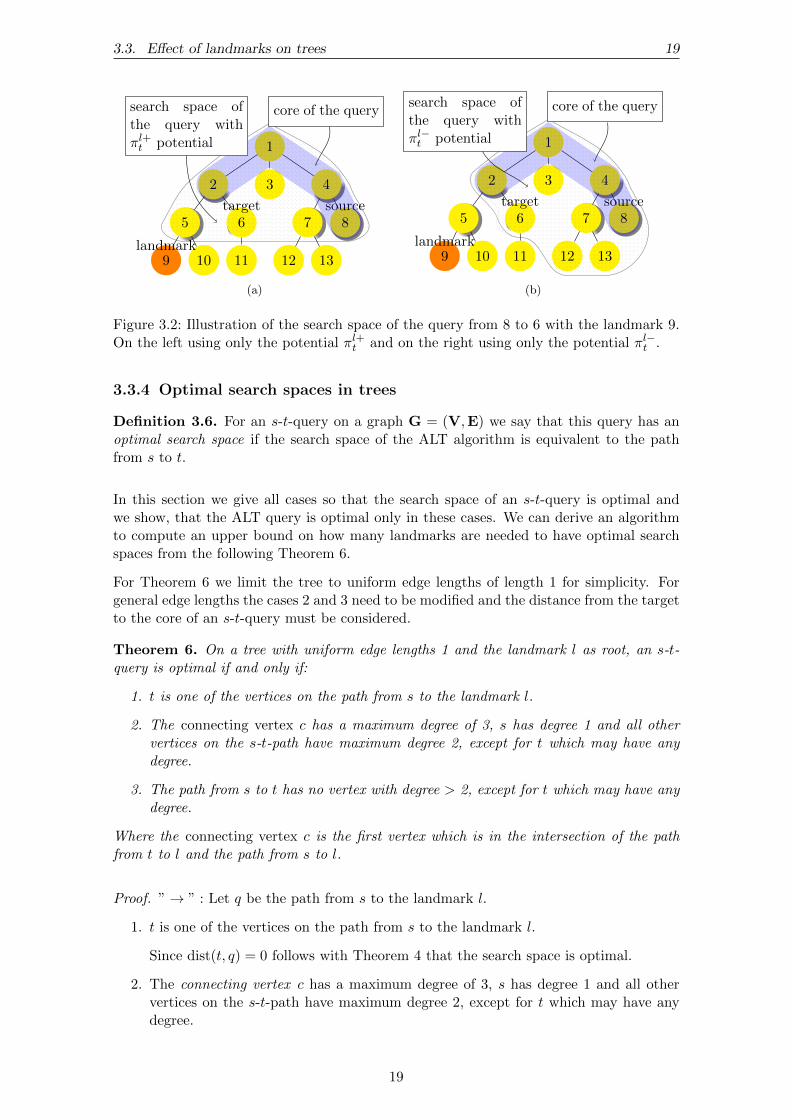
Figure 3.2: Illustration of the search space of the query from 8 to 6 with the landmark 9.On the left using only the potential πl+t and on the right using only the potential πl−t .

3.3.4 Optimal search spaces in trees

Definition 3.6. For an s-t-query on a graph G = (V,E) we say that this query has anoptimal search space if the search space of the ALT algorithm is equivalent to the pathfrom s to t.

In this section we give all cases so that the search space of an s-t-query is optimal andwe show, that the ALT query is optimal only in these cases. We can derive an algorithmto compute an upper bound on how many landmarks are needed to have optimal searchspaces from the following Theorem 6.

For Theorem 6 we limit the tree to uniform edge lengths of length 1 for simplicity. Forgeneral edge lengths the cases 2 and 3 need to be modified and the distance from the targetto the core of an s-t-query must be considered.

Theorem 6. On a tree with uniform edge lengths 1 and the landmark l as root, an s-t-query is optimal if and only if:

1. t is one of the vertices on the path from s to the landmark l.

2. The connecting vertex c has a maximum degree of 3, s has degree 1 and all othervertices on the s-t-path have maximum degree 2, except for t which may have anydegree.

3. The path from s to t has no vertex with degree > 2, except for t which may have anydegree.

Where the connecting vertex c is the first vertex which is in the intersection of the pathfrom t to l and the path from s to l.

Proof. ”→ ” : Let q be the path from s to the landmark l.

1. t is one of the vertices on the path from s to the landmark l.

Since dist(t, q) = 0 follows with Theorem 4 that the search space is optimal.

2. The connecting vertex c has a maximum degree of 3, s has degree 1 and all othervertices on the s-t-path have maximum degree 2, except for t which may have anydegree.

19

20 3. Landmarks

The source and all vertices except for the connecting vertex c must not be considered,since ALT can not reach vertices which are not on the s-t-path from them. Fromthe fact that the connecting vertex has degree 3, we know that the one adjacentvertex which is not on the s-t-path is on the path from the connecting vertex to thelandmark. That this vertex will not be settled follows from Theorem 5 which statesthat ALT will not search closer to the landmark then necessary

3. The path from s to t has no vertex with degree > 2, except for t which may haveany degree.

In this case ALT has only one possibility to settle vertices not on the s-t-path: Tosettle the adjacent vertex u of s which is not on q. Either this vertex u is on thepath from s to the landmark and therefore will not be settled according to Theorem5 or case 1 applies.

”← ” :

Let s-t be an optimal query and {s = v0, v1, . . . , vr = t} be the vertices on the path froms to t.

Assume that the s-t-path is not one of the cases 1, 2 or 3. Then, t is not on the path froms to l and only the following cases remain possible:

(i) t is in a subtree of s

(ii) t and s are connected through vertex c 6= l with degree ≥ 3.

(iii) t and s are connected through vertex c = l with degree ≥ 2.

We will show that all three cases result in a contradiction.

(i) t is in a subtree of s

If {v1, . . . , vr−1} are vertices with degree ≤ 2, then case 3 applies for s-t. Hence atleast one vertex in {v0, . . . , vr−1} has degree > 2. Let v be this vertex, then:

cost(v) = dist(s, v) + |dist(v, l)− dist(t, l)|∗= dist(s, v)− dist(v, l) + dist(t, l)

= dist(s, v) + dist(v, t)

= dist(s, t)

(3.9)

where∗= holds, since dist(t, l) > dist(v, l). v has at least 3 adjacent vertices, and at

least one vertex u which is not on the s-t-path with

cost(u) = dist(s, u) + | dist(u, l)− dist(t, l)|= dist(s, v) + 1− | dist(v, l) + 1− dist(t, l)|= dist(s, v) + 1 +−dist(v, l)− 1 + dist(t, l)

= dist(s, v) + dist(v, t)

= dist(s, t)

(3.10)

Since v is on the s-t-path, v must be settled and therefore u must be settled too,though it is not on the s-t-path. Hence the search space of the s-t-query is notoptimal.

(ii) t and s are connected through vertex c 6= l with degree ≥ 3.

If v0 has degree 1 and {v1, . . . , vr−1} has only one vertex with degree 3, then case 2applies. Otherwise s has degree > 1 or {v1, . . . , vr−1} has at least one vertex withdegree > 3 or more than one vertex with degree 3.

20


Let Cls,t be the core of the s-t-query, i.e. the intersection of the path from s to l andthe path from s to t. Since t is not in the path q from s to l, ALT searches all verticeswithin dist(t, Cls,t) ≥ 1 of the core of the s-t-path. Hence it is sufficient to show that

in each remaining case a vertex u exists with dist(Cls,t, u) ≤ dist(Cls,t, t).

If {v1, . . . , vr−1} has only one connecting vertex with degree 3 but v0 has a degree> 2, v0 is obviously in the core and has one adjacent vertex u which is not on thes-t-path. For u it holds that dist(Cls,t, u) = 1 ≤ dist(Cls,t, t) since the target has atleast distance 1 from the core. Contradiction since u is settled from ALT and not onthe s-t-path.

If {v1, . . . , vr−1} has at least one vertex v with degree > 3, then this vertex has atleast one adjacent vertex u which is not on the s-t-path and not on the s-l-path forwhich dist(Cls,t, u) = 1 ≤ dist(Cls,t, t). Contradiction since u is settled from ALT andnot on the s-t-path.

If {v1, . . . , vr−1} has more than one vertex with degree 3, then let v be the vertexwhich has one adjacent vertex u which is not on the s-t-path and not on the s-l-path(at least one must exist if more than one vertex with degree ≥ 3 is on the path).As in the other cases, this vertex u is in the ALT search space though not on thes-t-path which results in an contradiction.

(iii) t and s are connected through vertex c = l.

If s has degree 1 and the vertices {v1, . . . , vr−1} have degree 2, case 2 applies. Oth-erwise s has degree > 1 or {v1, . . . , vr−1} has at least one vertex with degree > 2. Asin case (ii) the target t is not in the core Cls,t of the s-t-query and hence it is sufficient

to show that one vertex u exists which is dist(Cls,t, u) ≤ 1 ≤ dist(Cls,t, t)

If s has degree > 1 the to s adjacent vertex u has dist(Cls,t, u) = 1 ≤ dist(Cls,t, t). Ifin {v1, . . . , vr−1} at least one vertex has degree > 2, then this vertex has an adjacentvertex u which is not on the s-t-path with dist(Cls,t, u) = 1 ≤ dist(pCls,t, t). In bothcases u is in the search space and the search space is not optimal. Contradiction.

With this knowledge, we can compute for each vertex, which s-t-paths are optimal if thisvertex is a landmark. By solving a set-covering problem we can then compute an upperbound on the smallest number of landmarks which are needed to obtain an optimal searchspace for all queries. Note that we could also use any known approximation algorithm forset-covering. This approach does not give the exact bound, since some s-t-paths which arenot optimal for one landmark can be optimal if another landmark (for which alone thiss-t-path is not optimal, too) is added.

3.3.5 On paths between landmarks

In this section we will examine the vertices on paths between two (or more) landmarkson trees. We will show that adding to the landmark set any vertex which is on a pathbetween some other landmarks, does not yield a reduction of the search space.

Theorem 7. Let G = (V,E) be a tree and L = {l1, . . . , lk} with k ≥ 2 a set of landmarks.W.l.o.g. be v on a path between l1 and l2. Then, the set L′ = {l1, . . . , lk, v} will notimprove the overall ALT search space.

Proof. Suppose the set L′ improves the resulting overall ALT search space, then theremust be one s-t-query q which is improved by the landmark v. Then, q must be improvedby one of the ways stated in Section 3.3.1 (i) and 3.3.2 (ii).

21

22 3. Landmarks

We will first consider case (i): The search space can only be improved in this case if thetarget t is closer to the core of the s-t-query than before. The core of the s-t-query is theintersection of the s-t-path and one of the paths from the source to the landmarks. Sincev is on a path between two landmarks, the core of the s-t-query can not be enlarged, sinceno more vertices than before can be in the intersection. Contradiction.

Consider now (ii): Then, the landmark v must exclude a subtree from the ALT searchspace, which is searched by the ALT algorithm if it only uses the set L as landmarks.From the s-t-path, only vertices which are not in the direction of one of the landmarks inL may be settled using L, therefore v must exclude at least one vertex from the searchspace which is not in direction on another landmark but in direction of v. Since v is onthe path between l1 and l2 this is not possible. If a vertex can be excluded from the searchspace using v it has already be excluded by l1 or l2. Contradiction.

Hence the overall search space with the set L′ is the same as with L.

With this proof we get the intuition, that in a tree, landmarks should only be placed inleaves. This intuition is correct, as the following corollary states.

Corollary. Let G = (V,E) be a tree. Then only leaves or the root if it has only one child,i.e. vertices with only one adjacent vertex, are in the optimal set of k landmarks for k ≥ 2.

Proof. We assume {l1, . . . , lk} with k ≥ 2 are optimal landmarks and let w.l.o.g l1 havemore than one adjacent vertex. If none of the adjacent vertices is on a path from l1 toanother landmark, then according to Theorem 7 l1 has no more effect since it is on at leastone path between two other landmarks. Hence let u be the adjacent vertex which is noton the path from l1 to any other landmark. Then, the set {u, l2, . . . , lk} is at least as goodas {l1, . . . , lk}.

In Figure 3.3 we illustrated how one can draw a tree so that one can easily see the distancefrom the target t to the source-landmark-path s-l for an s-t-query as well as which s-t-queries are yet optimal. Originating from the idea behind this illustration that all verticesbetween landmarks act as if they were landmarks which has been shown in Theorem 7 wewill introduce a new heuristic for the selection of a set of landmarks in Section 4.4.

22


8

4

2

5

10 11

1

3

6

12 13

7

14 15

9

(a)

18 1214

9

6

13

12

5

10 11

3

7

14 15

(b)

Figure 3.3: In both images we see the same complete binary tree with 15 vertices (instandard notation, 1 would be the root). On the left (a) the tree is drawn with onelandmark vertex 8 as root and on the right (b) the path from the landmark 8 to thelandmark 12 substitutes a root vertex.

23

4. Implementations and algorithms

In this Chapter we will first give another interpretation of the problem to select the land-marks, which will lead us to a binary linear program formulation. Afterwards we will givetwo formulations of a greedy algorithm which holds an approximation guarantee of e−1

e ofthe optimal solution. Then we will introduce a new heuristic and finally give a brute forcealgorithm to compute a optimal set of k landmarks.

4.1 Selecting landmarks as maximum coverage problem

In contrast to the problem MinALT defined in Chapter 3 we will first define the problemof maximum coverage (MaxCover) in this section and afterwards show that the problemMinALT can be reduced to the problem MaxCover.

Definition 4.1 (MaxCover). Given a set of elements {e1, . . . , er}, a collection S ={S1, . . . , Sn} of sets where Si ⊂ {e1, . . . , er} and an integer k, the problem MaxCoveris to find a subset S ′ ⊂ S with |S ′| ≤ k so that a maximum number of elements ei arecovered:

⋃Si∈S′ Si is maximal.

Such a set S ′ is called a set with maximum coverage.

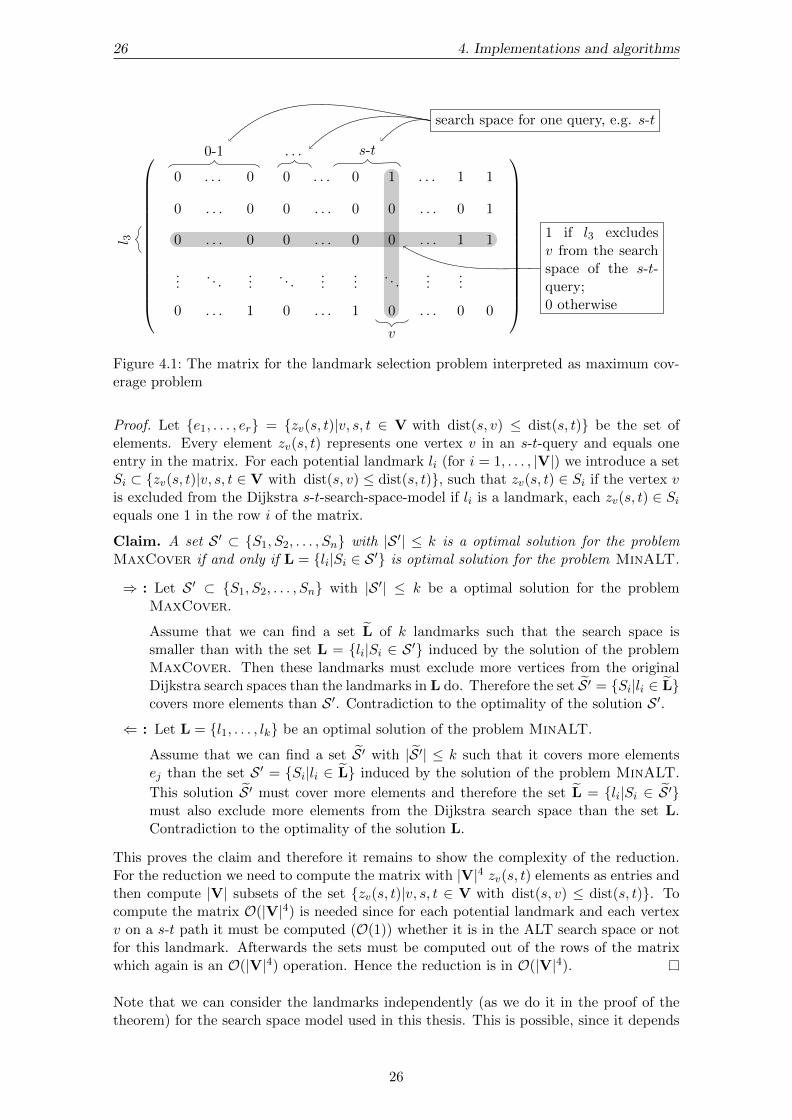
The idea of interpreting the problem of selecting k landmarks as a maximum coverageproblem is to compute, for each vertex v and each s-t-query, which vertices the vertexv would exclude from the Dijkstra search if it would be a landmark. Therefore we startby computing the Dijkstra search space for each s-t-query and setting up a |V |3 × |V |matrix with one column for each vertex in every Dijkstra search space and one row foreach vertex in V, interpreted as potential landmark. Each column is assigned to one vertexv in the Dijkstra search space of an s-t-query and each row to one potential landmark lias illustrated in Figure 4.1. Each entry of the matrix is initialized with 0.

Then, for each vertex v in the Dijkstra search space of an s-t-query we compute for everypotential landmark li if the ALT algorithm would visit v on the s-t-query when using lias landmark. If the ALT algorithm would not visit v using li (i.e. li would exclude v fromthe search space), we set the entry for row li in the column assigned to the vertex v to1. For this matrix, selecting k rows so that a maximum number of columns are covered isequivalent to the maximum coverage problem.

Theorem 8. There is an polynomial reduction from the problem MinALT to MaxCoverwith complexity in O(|V |4).

25

26 4. Implementations and algorithms

0 . . . 0 0 . . . 0 1 . . . 1 1

0 . . . 0 0 . . . 0 0 . . . 0 1

0 . . . 0 0 . . . 0 0 . . . 1 1

.... . .

.... . .

......

. . ....

...

0 . . . 1 0 . . . 1 0 . . . 0 0

search space for one query, e.g. s-t

1 if l3 excludesv from the searchspace of the s-t-query;0 otherwise

0-1 . . . s-t

v

l 3

Figure 4.1: The matrix for the landmark selection problem interpreted as maximum cov-erage problem

Proof. Let {e1, . . . , er} = {zv(s, t)|v, s, t ∈ V with dist(s, v) ≤ dist(s, t)} be the set ofelements. Every element zv(s, t) represents one vertex v in an s-t-query and equals oneentry in the matrix. For each potential landmark li (for i = 1, . . . , |V|) we introduce a setSi ⊂ {zv(s, t)|v, s, t ∈ V with dist(s, v) ≤ dist(s, t)}, such that zv(s, t) ∈ Si if the vertex vis excluded from the Dijkstra s-t-search-space-model if li is a landmark, each zv(s, t) ∈ Siequals one 1 in the row i of the matrix.

Claim. A set S ′ ⊂ {S1, S2, . . . , Sn} with |S ′| ≤ k is a optimal solution for the problemMaxCover if and only if L = {li|Si ∈ S ′} is optimal solution for the problem MinALT.

⇒ : Let S ′ ⊂ {S1, S2, . . . , Sn} with |S ′| ≤ k be a optimal solution for the problemMaxCover.

Assume that we can find a set L of k landmarks such that the search space issmaller than with the set L = {li|Si ∈ S ′} induced by the solution of the problemMaxCover. Then these landmarks must exclude more vertices from the originalDijkstra search spaces than the landmarks in L do. Therefore the set S ′ = {Si|li ∈ L}covers more elements than S ′. Contradiction to the optimality of the solution S ′.

⇐ : Let L = {l1, . . . , lk} be an optimal solution of the problem MinALT.

Assume that we can find a set S ′ with |S ′| ≤ k such that it covers more elementsej than the set S ′ = {Si|li ∈ L} induced by the solution of the problem MinALT.

This solution S ′ must cover more elements and therefore the set L = {li|Si ∈ S ′}must also exclude more elements from the Dijkstra search space than the set L.Contradiction to the optimality of the solution L.

This proves the claim and therefore it remains to show the complexity of the reduction.For the reduction we need to compute the matrix with |V|4 zv(s, t) elements as entries andthen compute |V| subsets of the set {zv(s, t)|v, s, t ∈ V with dist(s, v) ≤ dist(s, t)}. Tocompute the matrix O(|V|4) is needed since for each potential landmark and each vertexv on a s-t path it must be computed (O(1)) whether it is in the ALT search space or notfor this landmark. Afterwards the sets must be computed out of the rows of the matrixwhich again is an O(|V|4) operation. Hence the reduction is in O(|V|4).

Note that we can consider the landmarks independently (as we do it in the proof of thetheorem) for the search space model used in this thesis. This is possible, since it depends

26

4.2. Integer linear program 27

solely on the distance and the potential of a vertex whether it is in the search space ofan given s-t-query or not. For other models this is not necessarily possible as we showedin an example in Section 3.1 that the actual ALT search space increased for this exampleeven though we added one more landmark.

4.2 Integer linear program

For the problem MinALT of selecting k landmarks so that the search space of the ALTalgorithm is minimal, we can formulate a integer linear program by using the formulationof the problem as a maximum coverage problem MaxCover. In this chapter we will givea binary linear program using the search space model used throughout this thesis andintroduced in Section 3.1.

This approach models for each vertex v in any Dijkstra search space, which landmarksexclude this vertex v from the ALT search space. With the linear program, the set of klandmarks which excludes most vertices from the ALT search space is computed. Beforewe can formulate the binary linear program, we must preprocess the distances between allvertices in the graph. After that, let V(s, t) := {v ∈ V |dist(s, v) ≤ dist(s, t)} denote thesearch space model of an s-t-query using Dijkstra’s algorithm. These search spaces haveto be precomputed for every pair of vertices s and t ∈ V. For s,t ∈ V and v ∈ V(s, t) weuse the variables

zv(s, t) =

{0 v is not in the ALT search space model of the s-t-query

1 otherwise(4.1)

and variables L(v) being 1 if v is a landmark and 0 otherwise. Finally we let Lv(s, t)denote the set of landmarks l such that v is not in the ALT search-space-model of thes-t-query if landmark l is used. This set can be computed using only the precomputeddistances and the resulting potentials.

With these variables the binary linear program can be formulated as the following maxi-mization problem.

max∑

s,t∈V,v∈V(s,t)

zv(s, t) (4.2)

subject to

zv(s, t) ∈ [0, 1] for s, t ∈ V and v ∈ V(s, t) (4.3)

L(v) ∈ {0, 1} for v ∈ V (4.4)

zv(s, t) ≤∑

l∈Lv(s,t)

L(l) for s, t ∈ V and v ∈ V(s, t) (4.5)

∑v∈V

L(v) ≤ k (4.6)

In this linear programming formulation, we maximize over zv(s, t) for all vertices v in theDijkstra search space for all pairs (s,t). This implies a minimal overall search space of theALT-algorithm, since the overall search space of the ALT algorithm is the overall Dijkstrasearch space minus

∑s,t∈V,v∈V(s,t) zv(s, t).

It is sufficient to require, that the variable zv(s, t) must be in the interval from 0 to 1, sinceintegrality of zv(s, t) follows from the fact that we are maximizing the variables zv(s, t)and that they only appear in constraint (4.5) which has an integral right hand side if L(l)

27


is integral. Finally, constraint (4.6) requires the number of landmarks be smaller or equalto k.

A downside of this formulation is that this linear program is quite memory-consuming. Torepresent zv(s, t) for each vertex v in the Dijkstra search space model in every s-t-pair, |V|3variables are needed. For the set Lv(s, t) we need even O(|V |4) variables since for eachvertex v in the Dijkstra search space model in every s-t-pair a set of landmarks must bestored. Additionally we need to precompute |V| ∗ |V| distances, which is computationallyin the complexity of O(|V |3) (see Algorithm 4.1). The potential function can be computedout of the distances when needed since it does only depend on s, t, v and l whether l is inLv(s, t) or not.

4.3 The greedy algorithm

In order to describe the greedy algorithm, we will first describe two methods which areused in the greedy algorithm as well as for the brute force algorithm in Section 4.5.

The Algorithm 4.1 computes all-pair-shortest-paths, i.e. the distances between all pairs ofvertices, and is called Floyd-Warshall algorithm (Cormen et al., 2001). The complexity ofthis algorithm is O(|V|3).

Algorithm 4.1 Floyd-Warshall()

Require: A graph G = (V,E) with positive length function lenEnsure: dist(u, v) for all u, v ∈ V1: for all u ∈ V do2: for all v ∈ V do3: if (u, v) ∈ E then4: dist(u, v)← len(u, v)5: else6: dist(u, v)←∞7: for k = 1 . . . |V| do8: for all s ∈ V do9: for all t ∈ V do

10: dist(s, t)← min{dist(s, t), dist(s, k) + dist(k, t)}

To compute the search space for one pair of source and target vertices s and t the Algorithm4.2 is used. It requires precomputed distances between all pairs of vertices in V andcomputes the search space according to the model given in Section 3.1. The algorithm hasa complexity of O((|V| · k) + |V|) = O(|V| · k)

Algorithm 4.2 compute VL(s, t)(L, s, t)

Require: dist(u, v) for all u, v ∈ V, set of landmarks L, s, t ∈ VEnsure: correct set VL(s, t) of vertices in the search space of the s-t-query1: for all v ∈ V do2: πLt (v)← max

l∈L{dist(v, l)− dist(t, l),dist(l, t)− dist(l, v)}

3: for all v ∈ V do4: if dist(s, v) + πLt (v) ≤ dist(s, t) then5: VL(s, t)← VL(s, t) ∪ {v}

The greedy algorithm as it is given in Algorithm 4.3 computes the one vertex v whichminimizes the search space if added to the so far computed set L of landmarks in eachiteration. This vertex v is then added to the set L of landmarks. After k iterations Lconsists of k landmarks and is returned as the set of selected landmarks.

28

4.3. The greedy algorithm 29

Algorithm 4.3 Greedy(k)

Require: Integer k1: L← ∅2: Floyd-Warshall() {compute all-pair-shortest-paths}3: for all i = 1, . . . , k do4: for all l ∈ (V − L) do5: for all (s, t) ∈ V do6: compute VL(s, t)(L, s, t) {compute search space}7: sum[l] =

∑s,t∈V VL(s, t)

8: bestLM ← argmin{sum[l] | l ∈ (V − L)}9: L← L ∩ {bestLM}

10: return Set L of k landmarks

We can also formulate this greedy algorithm in a similar way as the integer linear programin Section 4.2. We no longer add the one vertex v to the set L of landmarks whichminimizes the resulting search space but the one which excludes most vertices from thesearch space resulting from the so far computed set of landmarks. Since these formulationsare equivalent both variants always choose the same vertices and hence result in the sameset of landmarks.

Algorithm 4.4 AlternativeGreedy(k)

Require: Integer k1: L← ∅2: Floyd-Warshall() {compute all-pair-shortest-paths}3: for all v ∈ V do4: sum[v] ← 05: min ← ∞6: minLm ← null7: for all i = 1, . . . , k do8: for all s ∈ V do9: for all t ∈ V do

10: for all v ∈ V do11: if dist(s, v) ≤ dist(s, t) then12: for all l ∈ V do13: potential ← max{dist(v, l)− dist(t, l), dist(l, t)− dist(l, v)}14: if dist(s, v) + potential ≤ dist(s, t) then15: sum[l] ← sum[l] + 116: for all l ∈ V do17: if sum[l] < min then18: min ← sum[l]19: minLm ← l20: L← L ∪ {l}21: return Set L of k landmarks

With the alternative formulation of the greedy algorithm as it is given in Algorithm 4.4we are able to interpret the algorithm as a greedy algorithm for the maximum coverageproblem. This problem is well known in literature and provides us with an approximationguarantee of (1 − e

1) = e−1e of the optimal solution for finding a set which excludes a

maximum number of vertices (Hochbaum, 1997), where e is Euler’s number.

Theorem 9 ((Hochbaum, 1997)). Let weight(GREEDY ) be the weight of the solution ofthe greedy algorithm for the problem MaxCover and weight(OPT ) be the weight of the

29


optimal solution for the same problem, then:

weight(GREEDY ) ≥ [1− (1− 1

k)k] · weight(OPT ) > (1− 1

e) · weight(OPT ) (4.7)

Corollary. Let coverage(GREEDY ) be the number of vertices which can be excluded fromthe Dijkstra search space in the greedy solution for the MinALT problem and coverage(OPT )be the number of vertices which can be excluded in the optimal solution of the same problem,then:

coverage(GREEDY ) ≥ [1− (1− 1

k)k] · coverage(OPT ) > (1− 1

e) · coverage(OPT ) (4.8)

Proof. The corollary follows directly from Theorem 9, since the equality of the problemsMaxCover and MinALT is shown in Theorem 8.

We also know that this is basically best we can do with the maximum coverage approach,since an approximation threshold of e−1e (up to low-order terms) is shown for the maximumcoverage problem (Feige, 1998).

4.4 A new heuristic

The greedy algorithm presented in the previous section may perform well, but its com-plexity as well as its memory requirements are high and therefore the algorithm will notbe applicable on real world data. Hence we will give another heuristic which has beeninspired by our understanding of the effects of landmarks on trees gained in Section 3.3.

As before, we will select one landmark at a time and therefore have k iterations to selectk landmarks.

For the first iteration, we temporarily add a random vertex to the set of landmarks whichwill be deleted after the first iteration. In each iteration we first add a dummy vertex r toV and edges (r, l) to E with length zero from this vertex r to the vertices l in the set Lof so far determined landmarks. We then build a search tree with the dummy vertex r asroot. In this search tree, we calculate a weight

weight(v) = dist(r, v) +∑

w child of v

weight(v) (4.9)

which is recursively computed in Algorithm 4.6 beginning at the root vertex. Then thealgorithm descends from the root vertex r always to the child with the highest weight(·)value until a leaf is reached. This leaf is selected and added to the set of landmarks asshown in Algorithm 4.7. In the first iteration, the random vertex added to the set oflandmarks before the iteration gets deleted again. Note that this way the algorithm isusually not selecting the node with the highest weight(·) value.

Unfortunately this heuristic could not be tested due to time limitations. In our opinion,the following improvements are interesting:

First, one minor improvement should be to start with a leaf vertex instead of a completelyrandomly determined vertex. An major improvement may be to introduce another set Lto store all vertices on a shortest path between two landmarks (including the landmarksitself) and then connect the dummy root vertex r to all vertices in the set L with edges ofzero length. This variant is inspired by the fact that in trees vertices on the path betweenlandmarks should not be added to the set of landmarks as it is stated in Section 3.3.5.

30

4.4. A new heuristic 31

Algorithm 4.5 weightedPaths(k)

Require: graph G = (V,E) and Integer k1: x ← random vertex2: L← {x}3: for i = 1 . . . k do4: V← V ∪ { root } {add an dummy vertex root}5: for all l ∈ L do6: E← E ∪ {(root,l)} {and edges with length 0 from root to all vertices in L}7: len(root,l) ← 08: Dijkstra((V,E),root) {calculate dist(root,v) for all v ∈ V}9: calculateWeights(root)

10: l ← maxWeightLeaf(root)11: L← L ∪ {l}12: if i = 1 then13: L← {l} {delete random vertex x}14: return Set L of k landmarks

Algorithm 4.6 calculateWeights(v)

Require: Vertex v1: weight(v)← dist(root,v)2: for all child w of v do3: weight(v)← weight(v)+calculateWeights(w)4: return weight(v)

Algorithm 4.7 maxWeightLeaf(v)

Require: Vertex v1: max ← 02: maxVertex ← null3: for all child w of v do4: if weight(w) > max then5: max ← weight(w)6: maxVertex ← w7: if maxVertex = null then8: return v9: return maxWeightLeaf(maxVertex)

31


4.5 The brute force algorithm

The brute force algorithm to solve the landmark selection problem given in Algorithm4.8 is similar to the greedy algorithm given in Algorithm 4.3, except for that we do notcalculate the resulting search space k · V times but

(|V|k

)times: Instead of computing

the next best landmark with smallest resulting search space for k iterations in the greedyalgorithm we compute the set L ⊂ V of k landmarks (of which

(|V|k

)different exist) with

the smallest resulting search space. As in the greedy algorithm we use Algorithm 4.1 tocompute all-pair-shortest-paths and Algorithm 4.2 to compute the search space for thes-t-query using a set L of landmarks.

Algorithm 4.8 BruteForceLandmarks(k)

Require: Integer k1: Floyd-Warshall()2: Lmin ← ∅3: min ← ∞4: for all subsets L ⊂ V with |L| = k do5: for all (s, t) ∈ V do6: compute VL(s, t)(L, s, t)7: sum ←

∑s,t∈V VL(s, t)

8: if sum < min then9: min ← sum

10: Lmin ← L11: return Lmin of optimal landmarks

Since(|V|k

)∈ θ(|V|k), the algorithm has a complexity of O(|V|3 + |V|k · k · (|V|2 · |V| · k+

|V|2)) = O(|V|k · k · |V|2 · |V| · k) = O(|V|k+3 · k2). Obviously, an algorithm with thiscomplexity is not able to handle large graphs, let alone real world road networks.

32

5. Experiments

We were provided with an existing C++ code which implements the heuristics used sofar like random, avoid, advanced avoid and maxCover from the Algorithmics I group atthe Institute of Theoretical Informatics at the Karlsruhe Institute of Technology. Addi-tionally we implemented the greedy algorithm 4.3 from Section 4.3 as well as a method tocalculate the resulting search space which has been used to measure the quality of a setof landmark. This method basically calls algorithm 4.2 for each pair s,t ∈ V and hencemeasures the quality way more precisely than the reduced costs method introduced byGoldberg (Goldberg and Werneck, 2005) - though unfortunately it is only applicable forsmall graphs due to its complexity. The integer linear program from Section 4.2 has beenimplemented in Java using cplex (ILOG, 2009) as solver for the integer linear program.

The hardware environment for the experiments was a server with two Intel Xeon E5340Quad-Core CPUs with 2.66Ghz per core and 6MB of cache per CPU. The server is equippedwith 32GB of memory. All implementations did only use one core while running, so thatseveral instances of the same or different programs ran simultaneously. Regarding thesoftware environment the server is running SUSE Linux 11.0 as operating system withkernel 2.6.25.20-0.5-default. The java virtual machine is running at version 1.6.0 17 andthe implementation in C++ has been compiled using gcc version 4.3.3 with parameters’-O4 -funroll-loops -DNDEBUG -DUNPACK’.

We were eager to try the methods on graphs as similar as possible to real world conditions.Due to the complexity and hence the resulting runtime and memory requirements forreal world graphs, we had to limit ourself to small parts of these real world graphs. Wegratefully acknowledge the support of PTV AG, Karlsruhe for providing us with real worldroad network graphs, though we were not able to use the whole graphs for the experiments.Instead we extracted strongly connected components from these graphs to obtain graphsof manageable sizes which are most likely connected.

In the following sections we will compare the heuristics used so far with the greedy algo-rithm as well as the integer linear program. Therefore we will first give a brief overviewon how the different heuristics work:random picks the amount of landmarks required as the set of landmarks randomly.avoid first grows a shortest path tree Tr with random root r in which for each iterationfor each vertex v the weight as difference between dist(r, v) and the lower bound inducedby the set L of so far selected landmarks. Then, the size of each vertex v is computed asthe sum of weight of the vertices in the subtree of v if there is no landmark in the subtree.

33

34 5. Experiments

If a landmark is in the subtree of v, the size of v is 0. Finally the algorithm traverses thetree starting at the vertex w with maximum size always to the child with the largest sizeuntil a leaf is reached. This leaf is added to the set of landmarks.advanced avoid is a variant of avoid which tries to compensate the main disadvantage ofavoid by exchanging the first landmarks selected by avoid by other landmarks later gen-erated by avoid.maxCover also tries to compensate the disadvantages of avoid by computing a set of land-marks 4 times bigger than needed using avoid. Out of these landmark candidates maxCoverselects the landmarks then through several attempts using a local search routine.

5.1 Comparison with the Integer Linear Program

Despite the progress linear program solver like cplex made in the past years, we havenot been able to apply our integer linear program to graphs bigger than around 125 to150 vertices when requiring the solver to finish within 6 hours. We may note that thoughthe linear program is quite memory consuming (for 150 vertices our linear program usesabout 10GB of main memory) this was not yet the limiting factor since even within thetime limit set to 6 hours there has been instances with at most 125 or 150 vertices whichcplex has not been able to solve optimally. For these instances no solution or if availablethe best feasible solution is given.

Since it is obviously not possible to test the linear program on real world graphs, we limitourself to a comparison of how good the solution of the heuristics used so far and thegreedy implementation is compared to the optimal solution computed by cplex using theinteger linear program.

The search space in the following Table 5.1 has been computed without considering thes-t-queries with dist(s, t) = ∞ at all, i.e. the search space of queries such that the targett is not reachable from the source s is not taken into account.

In the comparison in Table 5.1 we can see, that the quality of the generated landmarksimproves with the time needed to compute them. Overall we can say that the quality ofthe generated set of landmarks usually is in the following order

adv. avoid ≤ avoid ≤ maxCover ≤ greedy ≤ ILP

If we consider the time needed to generate the landmarks, we observe almost the reserveorder except for adv. avoid which is usually taking more time than avoid. On our graphswe can not see an improvement from advanced avoid over avoid, for most graphs we tested,advanced avoid has been worse than avoid.

We can also see that for most of our combination of graphs and generated landmarks thegreedy algorithm is as good as the optimal algorithm, though we suppose that for biggergraphs the gap between them is getting clearer (as we can see a first gap at the lux-graphwith 100 vertices).

5.2 Comparing the Greedy Algorithm

Even though the greedy algorithm is less complex than the brute force algorithm as wellas is requires less memory than the integer linear program, once again we are not ableto run this algorithm on real-world road-network graphs. On our configuration, the im-plementation of the greedy algorithm could at most be applied to compute around 12 to16 landmarks on a graph with 1500 vertices without exceeding the time limitations of 90hours.

34

5.2. Comparing the Greedy Algorithm 35

graphs deu lux

time search space time search space

50 vertices

avoid 0.0001 s 21,643 0.0001 s 26,897adv. avoid 0.0002 s 21,785 0.0003 s 27,945maxCover 0.0006 s 21,209 0.0005 s 26,396greedy 0.07814 s 20,689 0.1036 s 26,309ilp 33.420 s 20,689 34.548 s 26,309

100 vertices

avoid 0.0003 s 167,877 0.0003 s 179,275adv. avoid 0.0007 s 174,042 0.0009 s 188,275maxCover 0.001 s 156,353 0.00111 s 179,055greedy 1.6513 s 156,043 1.6618 s 178,359ilp 2h 4m 42s 156,043 10h 30m 47s 178,146

125 vertices

avoid 0.0005 s 278,486 0.0003 s 334,616adv. avoid 0.0008 s 291,885 0.0011 s 350,209maxCover 0.0013 s 263,089 0.0016 s 317,208greedy 3.4267 s 262,647 3.6162 s 308,232ilp 6h 1m 54s - (*) 6h 1m 54s - (*)

Table 5.1: Comparison of the heuristics used so far with the greedy algorithm and theinteger linear program solved with cplex on two different graphs. We generated for eachgraph and each method 4 landmarks. The heuristics have been run three times and amedian of the runs has been taken. (*) indicates that no binary solution has been foundin time.

Since we are not able to run the greedy algorithm on real-world road-networks, we limitedourself to compare to solution of the heuristics used so far to the one found by the greedyalgorithm and therefore get an idea of how good the heuristics are for bigger graphs thanthose solvable by the integer linear program.

The results given in Table 5.2 indicates the same order as the comparison on slightlysmaller graphs. Once again the greedy algorithm clearly dominates the other methodsconsidering the resulting search space. Compared to the search space of the maxCoverheuristic greedy as about 96 to 90 percent of the search space with the results indicatingthat the gap is getting bigger with larger graphs. Compared to the search space of theavoid heuristic the gap is with 94 to 88 percent of the search space a little bigger.

On the other hand, it is also obvious that if considering the time needed to compute thesolution the greedy can not compare with the other methods even on small graphs. For thesmall graphs under 100 vertices as compared in Table 5.1, the greedy algorithm is around1000 times slower than the heuristics, and for bigger graphs around 500-1500 vertices iteven is around one million times slower than the heuristics. As the asymptotic complexityimplies, the difference gets worse the bigger the graphs get.

So considering that we can only improve the overall search space by around 4 to 12 percent,the additionally needed amount of time is not paying off very well. In this setting, it wouldbe interesting to know how the heuristic proposed in Section 4.4 performs compared tothe so far leading heuristics like avoid, advanced avoid or maxCover.

35

36 5. Experiments

graphs deu lux

time search space time search space

500 vert. (370 vert.)

avoid 0.0064 s 8,798,842 0.0049 s 3,767,726adv. avoid 0.0091 s 9,115,170 0.0099 s 3,747,703maxCover 0.0333 s 8,532,156 0.0254 s 3,561,492greedy 1h 4m 6s 8,264,125 16m 19s 3,386,954

1000 vert.

avoid 0.0126 s 60,047,064 0.0127 s 69,765,480adv. avoid 0.0181 s 62,470,691 0.0182 s 69,831,648maxCover 0.0667 s 59,082,280 0.0709 s 66,182,107greedy 19h 40m 57s 56,708,679 15h 56m 34s 61,741,536

1500 vert.

avoid 0.0189 s 171,144,678 0.0193 s 200,782,618adv. avoid 0.0267 s 173,950,651 0.0276 s 209,381,550maxCover 0.1096 s 172,310,899 0.1022 s 191,656,773greedy 3d 17h 16m 48s 156,467,985 3d 14h 1m 19s 174,687,874

2000 vert.

avoid 0.0252 s 679,638,147 0.0266 s 410,382,530adv. avoid 0.0361 s 677,312,272 0.0375 s 437,572,399maxCover 0.1368 s 652,973,350 0.1402 s 401,492,530greedy - - - -

Table 5.2: Comparison of the heuristics used so far with the greedy algorithm on twodifferent graphs. During each run we generated 16 landmarks. The heuristics have beenrun three times and the median of the runs has been taken.

36

6. Conclusion

In this thesis we studied the preprocessing phase of the ALT algorithm. In particular, westudied the effects landmarks have on the ALT search space to get a better understandingand to improve the selection of landmarks. Though the effects of landmarks on the ALTsearch space on a general graph are quite complex, we were able to derive several resultsfor the effects on easier graph classes like chains and trees.Since we have been able to show that a new, less complex search space model for ALTis appropriate we were able to reduce the problem of the selection of k landmarks tothe maximum coverage problem. We are also able to formulate the greedy algorithm forthe selection of k landmarks as a maximum coverage problem, for which we could applyapproximation as well as inapproximability results. The formulation of the problem as amaximum coverage problem also results in an integer linear program we formulated andimplemented to solve the problem optimally for small graphs. We also gave an algorithmfor a new heuristic, which unfortunately could not be tested in this thesis but promisesgood results at least on trees due to its construction.

Future work: ALT is not the preprocessing based algorithm which results in the fastestquery times. In fact there are actually several algorithms resulting in faster query times.But in times where research is leading towards time-dependent routing, ALT, which hasthe advantage that it is not necessary to repeat the preprocessing everytime the length ofan edge has changed (though the search space may not be as good as before), is remaininginteresting. Hence it would be interesting to see how the search space changes for routingin time-dependent graphs as well as what can be done to select landmarks with an overall(i.e. for each possible variant of the graph) good performance.

37

Bibliography

Bauer, R., Columbus, T., Katz, B., Krug, M., and Wagner, D. (2010). Preprocessingspeed-up techniques is hard.

Bauer, R. and Delling, D. (2009). Sharc: Fast and robust unidirectional routing. ACMJournal of Experimental Algorithmics, 14.

Bellman, R. (1958). On a routing problem. Quarterly of Applied Mathematics, 16(1):87–90.

Cormen, T. H., Leiserson, C. E., Rivest, R. L., and Stein, C. (2001). Introduction toAlgorithms. MIT Press.

Delling, D., Sanders, P., Schultes, D., and Wagner, D. (2006). Highway hierarchies star.In 9th DIMACS Implementation Challenge.

Delling, D., Sanders, P., Schultes, D., and Wagner, D. (2009). Engineering route planningalgorithms. In Algorithmics of Large and Complex Networks, pages 117–139.

Dijkstra, E. W. (1959). A note on two problems in connexion with graphs. NumerischeMathematik, 1:269–271.

Feige, U. (1998). A threshold of ln n for approximating set cover. JOURNAL OF THEACM, 45:314–318.

Ford, L. and Fulkerson, D. (1962). Flows in Networks. Rand.

Geisberger, R., Sanders, P., Schultes, D., and Delling, D. (2008). Contraction hierarchies:Faster and simpler hierarchical routing in road networks. In WEA, pages 319–333.

Goldberg, A. and Werneck, R. (2005). Computing point-to-point shortest paths from ex-ternal memory. In Proceedings Workshop on Algorithm Engineering and Experiments(ALENEX 2005). SIAM.

Goldberg, A. V. and Harrelson, C. (2004). Computing the shortest path: A* search meetsgraph theory. Technical report.

Goldberg, A. V., Kaplan, H., and Werneck, R. F. F. (2007). Better landmarks withinreach. In WEA, pages 38–51.

Gutman, R. (2004). Reach-based routing: A new approach to shortest path algorithmsoptimized for road networks. In Proceedings 6th Workshop on Algorithm Engineeringand Experiments (ALENEX), pages 100–111. SIAM.

Hochbaum, D. S. H., editor (1997). Approximation algorithms for NP-hard problems. PWSPubl. Comp., Boston [u.a.].

Holzer, M., Schulz, F., and Wagner, D. (2009). Engineering multilevel overlay graphs forshortest-path queries. J. Exp. Algorithmics, 13:2.5–2.26.

ILOG, I. (2009). Cplex optimizer. online, http://www.ilog.com/products/cplex/.

39

http://www.ilog.com/products/cplex/

40 Bibliography

Schultes, D. and Sanders, P. (2007). Dynamic highway-node routing. In WEA, pages66–79.

Wagner, D. and Willhalm, T. (2007). Speed-up techniques for shortest-path computations.In STACS, pages 23–36.

40

On Preprocessing the ALT-Algorithm - Fabian Fuchs · In dieser Studienarbeit wurde die...

Documents

Transcript of On Preprocessing the ALT-Algorithm - Fabian Fuchs · In dieser Studienarbeit wurde die...