On Predictive Modeling for Claim Severity

Paper in Spring 2005 CAS Forum

Glenn MeyersISO Innovative Analytics

Predictive Modeling SeminarSeptember 19, 2005

Problems with Experience Rating for

Excess of Loss Reinsurance

• Use submission claim severity data– Relevant, but– Not credible– Not developed

• Use industry distributions– Credible, but– Not relevant (???)

General Problems withFitting Claim Severity Distributions

• Parameter uncertainty– Fitted parameters of chosen model are

estimates subject to sampling error.

• Model uncertainty– We might choose the wrong model. There is

no particular reason that the models we choose are appropriate.

• Loss development– Complete claim settlement data is not always

available.

Outline of Talk

• Quantifying Parameter Uncertainty– Likelihood ratio test

• Incorporating Model Uncertainty– Use Bayesian estimation with likelihood

functions– Uncertainty in excess layer loss estimates

• Bayesian estimation with prior models based on data reported to a statistical agent– Reflect insurer heterogeneity– Develops losses

The Likelihood Ratio Test

1Let ( ,..., ) be a set of observed

losses.nx xx

1Let ( ,..., ) be a parameter vector

for your chosen loss model.kp pp

ˆLet be the maximum likelihood

estimate of given .

p

p x

The Likelihood Ratio Test

0 1Test H : against H : * *p p p p

0

*

2

Theorem 2.10 in Klugman, Panjer & Willmot

If H is true then:

ˆ ln 2 ln ; ln ;

has a distribution with degrees

of freedom.

LR L p x L p x

k

2Use distribution to find critical values.

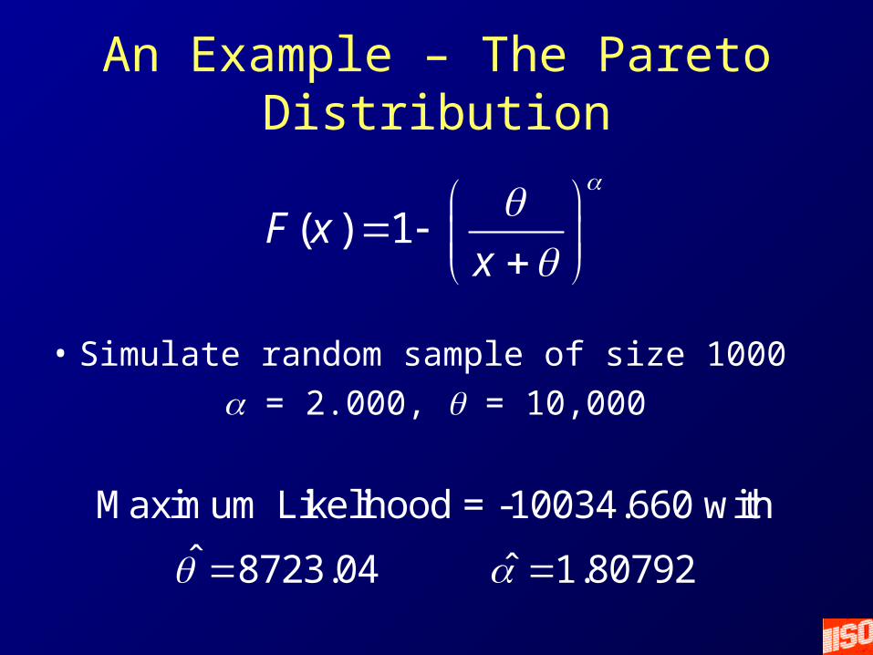
An Example – The Pareto Distribution

( ) 1F xx

• Simulate random sample of size 1000

= 2.000, = 10,000

Maximum Likelihood = -10034.660 with

ˆ ˆ8723.04 1.80792

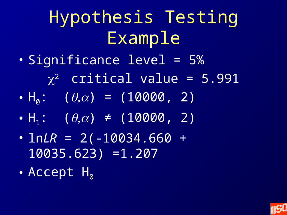
Hypothesis Testing Example

• Significance level = 5%

2 critical value = 5.991

• H0: () = (10000, 2)

• H1: () ≠ (10000, 2)

• lnLR = 2(-10034.660 + 10035.623) =1.207

• Accept H0

Hypothesis Testing Example

• Significance level = 5%

2 critical value = 5.991

• H0: () = (10000, 1.7)

• H1: () ≠ (10000, 1.7)

• lnLR = 2(-10034.660 + 10045.975) =22.631

• Reject H0

Confidence Region

• X% confidence region corresponds to the 1-X% level hypothesis test.

• The set of all parameters () that fail to reject corresponding H0.

• For the 95% confidence region:– (10000, 2.0) is in.– (10000, 1.7) out.

Confidence Region

Outer Ring 95%, Inner Ring 50%

0.0

0.5

1.0

1.5

2.0

2.5

0 5000 10000 15000Theta

Alp

ha

Grouped Data

• Data grouped into four intervals– 562 under 5000– 181 between 5000 and 10000– 134 between 10000 and 20000– 123 over 20000

• Same data as before, only less information is given.

Confidence Region for Grouped Data

Outer Ring 95%, Inner Ring 50%

0.0

0.5

1.0

1.5

2.0

2.5

0 5000 10000 15000Theta

Alp

ha

Confidence Region for Ungrouped Data

Outer Ring 95%, Inner Ring 50%

0.0

0.5

1.0

1.5

2.0

2.5

0 5000 10000 15000Theta

Alp

ha

Estimation with Model UncertaintyCOTOR Challenge – November 2004

• COTOR published 250 claims– Distributional form not revealed to participants

• Participants were challenged to estimate the cost of a $5M x $5M layer.

• Estimate confidence interval for pure premium

You want to fit a distribution to 250 Claims

• Knee jerk first reaction, plot a histogram.

0 1 2 3 4 5 6 7

x 106

0

50

100

150

200

250

Claim Amount

Cou

nt

Histogram of Cotor Data

This will not do! Take logs• And fit some standard distributions.

6 7 8 9 10 11 12 13 14 15 160

0.05

0.1

0.15

0.2

0.25

0.3

0.35

Log of Claim Amounts

Den

sity

lcotor data

lognormal

gamma

Weibull

Still looks skewed. Take double logs.

• And fit some standard distributions.

1.8 2 2.2 2.4 2.6 2.80

0.5

1

1.5

2

2.5

log log of Claim Amounts

Den

sity

llcotor data

Lognormal

Gamma

Weibull

Still looks skewed. Take triple logs.• Still some skewness. • Lognormal and gamma fits look somewhat better.

0.55 0.6 0.65 0.7 0.75 0.8 0.85 0.9 0.95 10

1

2

3

4

5

Triple log of Claim Amounts

Den

sity

lllcotor data

Lognormal

Gamma

Normal

Candidate #1Quadruple lognormal

Distribution: Lognormal Log likelihood: 283.496 Domain: 0 < y < Inf Mean: 0.738351 Variance: 0.006189 Parameter Estimate Std. Err. Mu -0.30898 0.00672 sigma 0.106252 0.004766 Estimated covariance of parameter estimates: mu sigma Mu 4.52E-05 1.31E-19 Sigma 1.31E-19 2.27E-05

Candidate #2Triple loggamma

Distribution: Gamma Log likelihood: 282.621 Domain: 0 < y < Inf Mean: 0.738355 Variance: 0.00615 Parameter Estimate Std. Err. A 88.6454 7.91382 B 0.008329 0.000746 Estimated covariance of parameter estimates: a b A 62.6286 -0.00588 B -0.00588 5.56E-07

Candidate #3Triple lognormal

All three cdf’s are within confidence interval for the quadruple lognormal.

0.55 0.6 0.65 0.7 0.75 0.8 0.85 0.9 0.95 10

0.1

0.2

0.3

0.4

0.5

0.6

0.7

0.8

0.9

1

Triple log of Claim Amounts

Cum

ulat

ive

prob

abili

ty

lllcotor data

Lognormal

confidence bounds (Lognormal)

Gamma

Normal

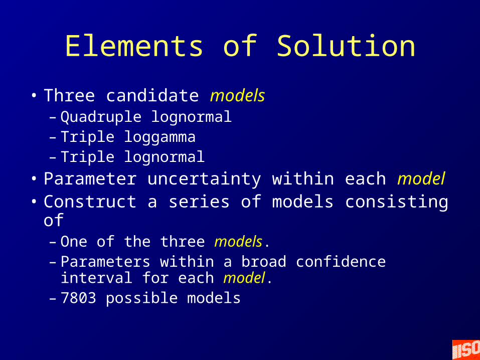
Elements of Solution

• Three candidate models– Quadruple lognormal– Triple loggamma– Triple lognormal

• Parameter uncertainty within each model• Construct a series of models consisting of

– One of the three models.– Parameters within a broad confidence interval

for each model. – 7803 possible models

Steps in Solution

• Calculate likelihood (given the data) for each model.

• Use Bayes’ Theorem to calculate posterior probability for each model– Each model has equal prior probability.

Posterior model|data Likelihood data|model Prior model

Steps in Solution

• Calculate layer pure premium for 5 x 5 layer for each model.

• Expected pure premium is the posterior probability weighted average of the model layer pure premiums.

• Second moment of pure premium is the posterior probability weighted average of the model layer pure premiums squared.

CDF of Layer Pure Premium

Probability that layer pure premium ≤ x

equals

Sum of posterior probabilities for which the

model layer pure premium is ≤ x

Numerical Results

Mean 6,430 Standard Deviation 3,370 Median 5,780

Range Low at 2.5% 1,760 High at 97.5% 14,710

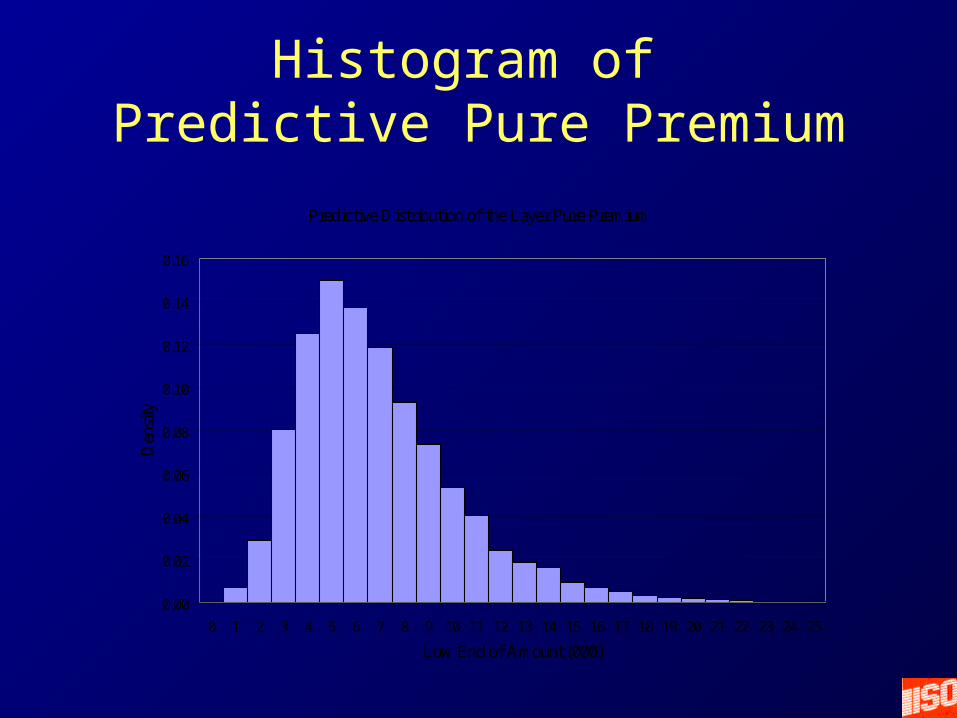
Histogram of Predictive Pure Premium

Predictive Distribution of the Layer Pure Premium

0.00

0.02

0.04

0.06

0.08

0.10

0.12

0.14

0.16

0 1 2 3 4 5 6 7 8 9 10 11 12 13 14 15 16 17 18 19 20 21 22 23 24 25

Low End of Amount (000)

Den

sity

Example with Insurance Data

• Continue with Bayesian Estimation

• Liability insurance claim severity data

• Prior distributions derived from models based on individual insurer data

• Prior models reflect the maturity of claim data used in the estimation

Initial Insurer Models

• Selected 20 insurers– Claim count in the thousands

• Fit mixed exponential distribution to the data of each insurer

• Initial fits had volatile tails

• Truncation issues– Do small claims predict likelihood of large

claims?

Initial Insurer Models

0

5,000

10,000

15,000

20,000

25,000

30,000

35,000

40,000

45,000

1,000 10,000 100,000 1,000,000 10,000,000

Loss Amount - x

Lim

ited

Ave

rage

Sev

erit

y

Low Truncation Point

0

500

1,000

1,500

2,000

2,500

3,000

3,500

4,000

4,500

5,000

0.00 0.05 0.10 0.15 0.20 0.25 0.30 0.35 0.40

Probability That Loss is Over 5,000

500

x 5

00 L

ayer

Ave

rage

Sev

erit

y

High Truncation Point

0

500

1,000

1,500

2,000

2,500

3,000

3,500

4,000

4,500

5,000

0.00 0.01 0.02 0.03 0.04 0.05 0.06 0.07

Probability That Loss is Over 100,000

500

x 5

00 L

ayer

Ave

rage

Sev

erit

y

Selections Made

• Truncation point = $100,000

• Family of cdf’s that has “correct” behavior– Admittedly the definition of “correct” is

debatable, but– The choices are transparent!

Selected Insurer Models

0

5,000

10,000

15,000

20,000

25,000

30,000

35,000

40,000

45,000

100,000 1,000,000 10,000,000

Loss Amount - x

Lim

ited

Ave

rage

Sev

erit

y

Selected Insurer Models

0

1,000

2,000

3,000

4,000

5,000

6,000

0.00 0.01 0.01 0.02 0.02 0.03 0.03 0.04 0.04 0.05

Probability That Loss is Over 100,000

500

x 50

0 L

ayer

Ave

rage

Sev

erit

y

Each model consists of

1. The claim severity distribution for all claims settled within 1 year

2. The claim severity distribution for all claims settled within 2 years

3. The claim severity distribution for all claims settled within 3 years

4. The ultimate claim severity distribution for all claims

5. The ultimate limited average severity curve

Three Sample Insurers Small, Medium and Large

• Each has three years of data

• Calculate likelihood functions– Most recent year with #1 on prior slide– 2nd most recent year with #2 on prior slide– 3rd most recent year with #3 on prior slide

• Use Bayes theorem to calculate posterior probability of each model

Formulas for Posterior Probabilities

, 1 ,

, ,, 11

AY m i AY m ii AY m

AY m

F x F xP

F x

,9 3

, ,1 1

i AYn

m i AY mi AY

l P

Posterior( ) Prior( )mm l m

Model (m) Cell Probabilities

Likelihood (m)

Using Bayes’ Theorem

Number of claims

ResultsTaken from

paper.

IntervalLower Claim Prior Posterior $500K x $1M x

Lags Bound Count Model # Probability $500K $1M1 100,000 15 1 0.016406 763 5411 200,000 2 2 0.041658 911 6451 300,000 1 3 0.089063 1,153 6821 400,000 2 4 0.130281 1,224 7961 500,000 0 5 0.157593 1,281 9121 750,000 0 6 0.110614 1,390 9781 1,000,000 0 7 0.075702 1,494 1,0401 1,500,000 0 8 0.053226 1,587 1,0951 2,000,000 0 9 0.080525 1,849 1,328

10 0.104056 2,069 1,52311 0.129925 2,417 1,828

1-2 100,000 40 12 0.010896 2,598 1,9161-2 200,000 10 13 0.000007 2,788 1,9221-2 300,000 1 14 0.000009 3,004 2,1241-2 400,000 0 15 0.000011 3,202 2,3091-2 500,000 2 16 0.000013 3,382 2,4771-2 750,000 0 17 0.000014 3,543 2,6281-2 1,000,000 2 18 0 4,058 3,2111-2 1,500,000 0 19 0 4,663 3,7841-2 2,000,000 0 20 0 5,354 4,440

1,572 1,1131-3 100,000 76 463 3851-3 200,000 261-3 300,000 111-3 400,000 31-3 500,000 81-3 750,000 01-3 1,000,000 01-3 1,500,000 01-3 2,000,000 0

Posterior MeanPosterior Std. Dev.

Exhibit 1 – Small InsurerLayer Pure Premium

Formulas for Ultimate Layer Pure Premium

• Use #5 on model (3rd previous) slide to calculate ultimate layer pure premium

20

=1

202 2

=1

Posterior Mean = Layer Pure Premium( ) Posterior( ).

Posterior Standard Deviation =

Layer Pure Premium( ) Posterior( ) Posterior Mean .

m

m

m m

m m

Results

• All insurers were simulated from same population.

• Posterior standard deviation decreases with insurer size.

$500K x $1M x $500K x $1M x $500K x $1M x$500K $1M $500K $1M $500K $1M

1,572 1,113 1,344 909 1,360 966463 385 278 245 234 188

Small Insurer Medium Insurer Large Insurer

Posterior MeanPosterior Std. Dev.

Layer Pure PremiumLayer Pure Premium Layer Pure Premium

Possible Extensions

• Obtain model for individual insurers

• Obtain data for insurer of interest

• Calculate likelihood, Pr{data|model}, for each insurer’s model.

• Use Bayes’ Theorem to calculate posterior probability of each model

• Calculate the statistic of choice using models and posterior probabilities– e.g. Loss reserves