On Multidimensional Item Response Theory: A Coordinate-Free Approach

July 2007 RR-07-30

ResearchReport

Tamás Antal

Research & Development

On Multidimensional Item Response Theory: A Coordinate-Free Approach

Tamás Antal

ETS, Princeton, NJ

July 2007

As part of its educational and social mission and in fulfilling the organization's nonprofit charter

and bylaws, ETS has and continues to learn from and also to lead research that furthers

educational and measurement research to advance quality and equity in education and assessment

for all users of the organization's products and services.

ETS Research Reports provide preliminary and limited dissemination of ETS research prior to

publication. To obtain a PDF or a print copy of a report, please visit:

http://www.ets.org/research/contact.html

Copyright © 2007 by Educational Testing Service. All rights reserved.

ETS and the ETS logo are registered trademarks of Educational Testing Service (ETS).

Abstract

A coordinate-free definition of complex-structure multidimensional item response theory

(MIRT) for dichotomously scored items is presented. The point of view taken emphasizes the

possibilities and subtleties of understanding MIRT as a multidimensional extension of the classical

unidimensional item response theory models. The main theorem of the paper is that every

monotonic MIRT model looks the same; they are all trivial extensions of univariate item response

theory.

Key words: MIRT, geometric methods, compensatory models

i

Acknowledgments

The author would like to extend his gratitude to Paul Holland for his the insights and constant

encouragement. The author is also indebted to Henry Chen for fruitful discussions. This paper

was inspired by a thought-provoking presentation by Mark Reckase at ETS in September 2006.

The author is indebted for the lively discussion during this presentation. Andreas Oranje and

Shelby Haberman provided useful reviews of the manuscript.

ii

1 Introduction

Complex-structure multidimensional item response theory (MIRT) is built on the idea that

a single item, however simple it might be, carries the possibility of an inner structure. In usual

terminology one speculates that it is possible to measure several cognitive areas with one item.

The number of cognitive areas so measured may vary among items, even though usual models

assume that it is fixed for a collection of items (a test) and let a factor analysis type procedure

decide on the number and mixture of cognitive areas measurable by the items.

The point of view taken in this note is that any unidimensional item response theory (IRT)

model can be thought of as a specialization of an MIRT model. Hence, the major task is to identify

how much of the well-established tools and nomenclature of unidimensional IRT can be preserved

in the multidimensional context and, from the other direction, how different multidimensional

notions may specialize to the same unidimensional entity. When the latter happens, that is

when two different multidimensional objects yield the same unidimensional specialization, then

both multidimensional notions could be considered proper generalizations of the underlying

unidimensional quantity. A careful study should then be devised to decide which generalization is

more appropriate with respect to the application at hand.

There is, on the other hand, the possibility of not finding proper multidimensional

generalization for some unidimensional notions. This topic also deserves careful research and

understanding.

This paper only considers what is termed complex-structure MIRT. Usually, IRT models have

two components: the item likelihood and the population distribution. In simple-structure MIRT,

one item represents only one dimension and without a multivariate population distribution the

entire likelihood of the model would factor as a product of univariate pieces. In complex-structure

MIRT, this factorization is impossible, by definition, irrespective of population model chosen.

The structure of the paper is as follows: a short overview of unidimensional IRT is followed

by the absolute, that is, coordinate-free definition of MIRT. The connection with the usual

approach is also shown via a discussion of two widely accepted models. Then the development

of the main thesis follows. This paper proves that MIRT models are all alike and they all can

be obtained as a trivial extension of an appropriate unidimensional IRT model. Two sections on

some thoughts about capturing cognitive dimensions and on understanding the role of the notion

of dimension-wise independence close the presentation.

1

2 Unidimensional Item Response Theory

To make the generalization to the multidimensional framework easier, some features of

unidimensional IRT are summarized first. Measurement takes place during the formation of

the response matrix X ∈ MN×I(N) with elements xni ∈ N for student n = 1, . . . , N and item

i = 1, . . . , I. In a dichotomous setting (which is assumed throughout the paper to simplify the

presentation), xni = 1 if student n responded correctly to item i, otherwise it is zero. As a major

simplification of the modeling of the cognitive process, it is assumed that students response to an

item is stochastically determined by students ability θn and item parameters βi := (ai, bi, ci) via

the item response function (Birnbaum, 1968).

P 3pl(θn, βi) := Prob(xni = 1 | θn, βi) = ci +1− ci

1 + e−ai(θn−bi). (1)

There are, of course, many different item response functions in use: the three-parameter logistic

(3PL) model is chosen here only as an illustration. The other substantial simplification used in

building the model is the assumption of independence of conditional probabilities P 3plni across an

arbitrary subset S ⊂ {1, . . . , N} × {1, . . . , I} of student-item pairs.

The two most popular models built out of these blocks are the joint unidimensional IRT and

the marginal unidimensional IRT. Joint IRT states that the total likelihood depends explicitly on

the ability of the given students:

Ljoint(X; Θ,B) =∏n,i

P 3pl(θn, βi)xni(1− P 3pl(θn, βi))1−xni (2)

with corresponding log-likelihood:

Ljoint(X; Θ,B) =∑n,i

xni log(P 3pl(θn, βi)) + (1− xni) log(1− P 3pl(θn, βi)). (3)

Here, Θ and B are the collections of all abilities and item parameters, respectively.

In marginal theory, the likelihood depends only on the distributional properties of student’s

population:

Lmarg(X;B,Φ) =∏n

∫R

∏i

P 3pl(θ, βi)xni(1− P 3pl(θ, βi))1−xnidµn(θ) (4)

with log-likelihood

Lmarg(X;B,Φ) =∑

n

log∫

R

∏i

P 3pl(θ, βi)xni(1− P 3pl(θ, βi))1−xnidµn(θ), (5)

2

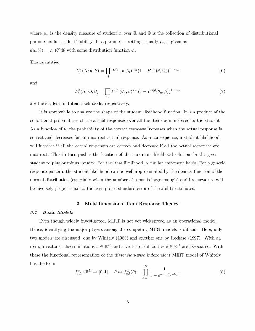
where µn is the density measure of student n over R and Φ is the collection of distributional

parameters for student’s ability. In a parametric setting, usually µn is given as

dµn(θ) = ϕn(θ)dθ with some distribution function ϕn.

The quantities

Lstn (X; θ,B) =

∏i

P 3pl(θ, βi)xni(1− P 3pl(θ, βi))1−xni (6)

and

Liti (X; Θ, β) =

∏n

P 3pl(θn, β)xni(1− P 3pl(θn, β))1−xni (7)

are the student and item likelihoods, respectively.

It is worthwhile to analyze the shape of the student likelihood function. It is a product of the

conditional probabilities of the actual responses over all the items administered to the student.

As a function of θ, the probability of the correct response increases when the actual response is

correct and decreases for an incorrect actual response. As a consequence, a student likelihood

will increase if all the actual responses are correct and decrease if all the actual responses are

incorrect. This in turn pushes the location of the maximum likelihood solution for the given

student to plus or minus infinity. For the item likelihood, a similar statement holds. For a generic

response pattern, the student likelihood can be well-approximated by the density function of the

normal distribution (especially when the number of items is large enough) and its curvature will

be inversely proportional to the asymptotic standard error of the ability estimates.

3 Multidimensional Item Response Theory

3.1 Basic Models

Even though widely investigated, MIRT is not yet widespread as an operational model.

Hence, identifying the major players among the competing MIRT models is difficult. Here, only

two models are discussed, one by Whitely (1980) and another one by Reckase (1997). With an

item, a vector of discriminations a ∈ RD and a vector of difficulties b ∈ RD are associated. With

these the functional representation of the dimension-wise independent MIRT model of Whitely

has the form

fwa,b : RD → [0, 1], θ 7→ fw

a,b(θ) =D∏

d=1

11 + e−ad(θd−bd)

. (8)

3

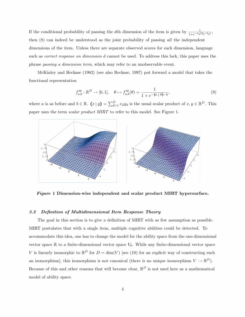
If the conditional probability of passing the dth dimension of the item is given by 11+e−ad(θd−bd) ,

then (8) can indeed be understood as the joint probability of passing all the independent

dimensions of the item. Unless there are separate observed scores for each dimension, language

such as correct response on dimension d cannot be used. To address this lack, this paper uses the

phrase passing a dimension term, which may refer to an unobservable event.

McKinley and Reckase (1982) (see also Reckase, 1997) put forward a model that takes the

functional representation

fspa,b : RD → [0, 1], θ 7→ fsp

a,b(θ) =1

1 + e−〈〈a θ〉〉−b, (9)

where a is as before and b ∈ R. 〈〈x y〉〉 =∑D

d=1 xdyd is the usual scalar product of x, y ∈ RD. This

paper uses the term scalar product MIRT to refer to this model. See Figure 1.

-4-2

02

4-4

-2

0

2

4

00.250.5

0.751

-4-2

02

4

-4-2

02

4-4

-2

0

2

4

00.250.5

0.751

-4-2

02

4

Figure 1 Dimension-wise independent and scalar product MIRT hypersurface.

3.2 Definition of Multidimensional Item Response Theory

The goal in this section is to give a definition of MIRT with as few assumption as possible.

MIRT postulates that with a single item, multiple cognitive abilities could be detected. To

accommodate this idea, one has to change the model for the ability space from the one-dimensional

vector space R to a finite-dimensional vector space Vθ. While any finite-dimensional vector space

V is linearly isomorphic to RD for D = dim(V ) [see (10) for an explicit way of constructing such

an isomorphism], this isomorphism is not canonical (there is no unique isomorphism V → RD).

Because of this and other reasons that will become clear, RD is not used here as a mathematical

model of ability space.

4

The reader unfamiliar with these notions is referred to Halmos (1974) for an excellent

introduction to linear algebra. Also, an intuitive understanding of the basic notions of smooth

manifolds should help understanding of what follows, although it not strictly necessary. Among

the many fine references to the topic, the interested reader may find Warner (1971) useful.

The basic object in unidimensional IRT is the item response function (IRF) and its

graph, the item response curve (IRC). The graph of a function f : A → B is a subset

graph(f) = {(x, f(x)) ∈ A×B | x ∈ A} of A×B. IRC is a one-dimensional smooth submanifold

of R × [0, 1]. While there is a scaling freedom even in the one-dimensional case (e.g., the

[in]famous 1.7 multiplier in the logistic models), the possibility of ambiguous interpretation is

minimal and one may use the functional (IRF) and the geometrical (IRC) representation almost

interchangeably.

In the multidimensional case, however, the matter is not so straightforward. As this paper

shows, the functional representation and the geometric representations are different in a subtle

way. One way to keep the presentation coordinate-free in multidimensional IRT is to postulate

that the theory is given by an item response hypersurface (IRHS). As in the unidimensional case,

the IRHS is used to express the probability of correct response given an ability in Vθ.

Before this paper defined this notion, some notations should be fixed. For any v ∈ Vθ, the ray

of v is defined to be the line R · v in Vθ determined by v: R · v = {λv ∈ Vθ | λ ∈ R}. Similarly, for

v, w ∈ Vθ, the v-directed line going through w is defined by

w + R · v = {w + λv ∈ Vθ | λ ∈ R}.

For the notion of IRHS, there is then the following:

Definition 1 A dichotomous item response hypersurface (IRHS) is a D = dim(Vθ) dimensional

smooth submanifold M of Vθ × [0, 1], so that for any two vectors v, w ∈ Vθ the intersection of

(w + R · v)× [0, 1] and M is a graph of a monotonic function w + R · v → [0, 1].

A MIRT model is given when an IRHS is given.

Note, that while w + R · v is not canonically isomorphic to R, monotonicity of the map

fv,w : w + R · v → [0, 1], λ 7→ fv,w(w + λv)

can be unambiguously defined by requiring that either fv,w(w + λv) ≤ fv,w(w + µv) or

5

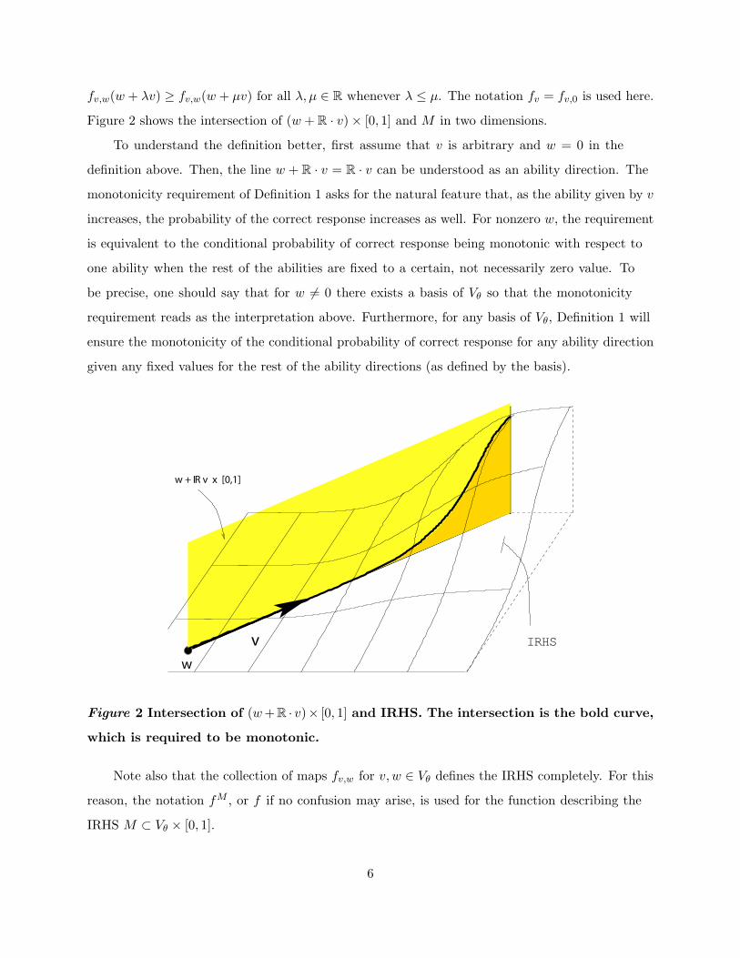
fv,w(w + λv) ≥ fv,w(w + µv) for all λ, µ ∈ R whenever λ ≤ µ. The notation fv = fv,0 is used here.

Figure 2 shows the intersection of (w + R · v)× [0, 1] and M in two dimensions.

To understand the definition better, first assume that v is arbitrary and w = 0 in the

definition above. Then, the line w + R · v = R · v can be understood as an ability direction. The

monotonicity requirement of Definition 1 asks for the natural feature that, as the ability given by v

increases, the probability of the correct response increases as well. For nonzero w, the requirement

is equivalent to the conditional probability of correct response being monotonic with respect to

one ability when the rest of the abilities are fixed to a certain, not necessarily zero value. To

be precise, one should say that for w 6= 0 there exists a basis of Vθ so that the monotonicity

requirement reads as the interpretation above. Furthermore, for any basis of Vθ, Definition 1 will

ensure the monotonicity of the conditional probability of correct response for any ability direction

given any fixed values for the rest of the ability directions (as defined by the basis).

IR v x [0,1]w +

vw

IRHS

Figure 2 Intersection of (w+R · v)× [0, 1] and IRHS. The intersection is the bold curve,

which is required to be monotonic.

Note also that the collection of maps fv,w for v, w ∈ Vθ defines the IRHS completely. For this

reason, the notation fM , or f if no confusion may arise, is used for the function describing the

IRHS M ⊂ Vθ × [0, 1].

6

One may be tempted to object to the use of notions like manifold and hypersurfaces. It is

very important to note, however, that the conditional probability of correct response has been

given by a hypersurface in the usual MIRT literature as well. One major difference in terminology

is that it was still called surface in any dimension, which is a correct usage only in Dimension 2.

In higher dimensions, the object at hand is a hypersurface, a special case of higher dimensional

manifolds.

A basis v = (v1, . . . , vD) in Vθ defines a unique isomorphism

iv : Vθ → RD,

D∑i=1

λivi 7→D∑

i=1

λiei, (λi ∈ R), (10)

where (ei)Di=1 is the standard basis of RD: (ei)j = δij (δij is the Kronecker delta). This

isomorphism can be trivially extended to a diffeomorphism

ψv : Vθ × [0, 1] → RD × [0, 1], (v, t) 7→ (iv(v), t) (11)

and via this diffeomorphism the IRHS may be transferred from Vθ × [0, 1] to RD × [0, 1]. Now, in

RD × [0, 1] the image of the IRHS may be given by the graph of a smooth function f : RD → [0, 1].

Note, however, the important difference between using a functional representation like this latter

one and using the hypersurface representation directly in Vθ × [0, 1]. The functional representation

depends on the basis chosen to establish the diffeomorphism ψv and different bases may result in

different functional representations.

It is tempting to extend this definition to polytomous multidimensional items by defining the

polytomous collection of item response hypersurfaces for a polytomous item by requiring that the

above discussed intersection be a collection of unidimensional polytomous item response curves

as produced by some unidimensional polytomous IRT model (e.g., Muraki’s [1992) partial credit

model). The investigation of this possibility is postponed for a forthcoming paper.

3.3 Properties of Item Response Hypersurfaces

This section proves the main theorem of the paper. For the sake of transparency, this section

starts with the two-dimensional case, which is then followed by the more involved general theory.

3.3.1 Two-Dimensional Case

Using the monotonicity of the model, it is possible to prove an interesting elementary

property.

7

Lemma 1 In any two-dimensional MIRT model, there exists a line in Vθ through the origin so

that fv is constant.

Proof: Choose a vector, v ∈ Vθ. Note that if infλ∈R

fv(λv) = supλ∈R

fv(λv), the lemma is proved and

the sought after line is R · v. Therefore, one may assume that infλ∈R

fv(λv) < supλ∈R

fv(λv). For such a

vector, either limλ→∞

fv(λv) = supλ∈R

fv(λv) or limλ→−∞

fv(λv) = supλ∈R

fv(λv). Let P be the set of vectors

satisfying the first and N be the set of vectors satisfying the second condition. Both of these sets

are nonempty, and by continuity, both sets are open. Also, they are clearly disjointed. Therefore,

there is a vector u ∈ Vθ so that u /∈ N ∪ P . Along the line R · u the function f is constant. �

Note that the proof only uses monotonicity with w = 0. Utilizing it for general w, the same

argument provides the following:

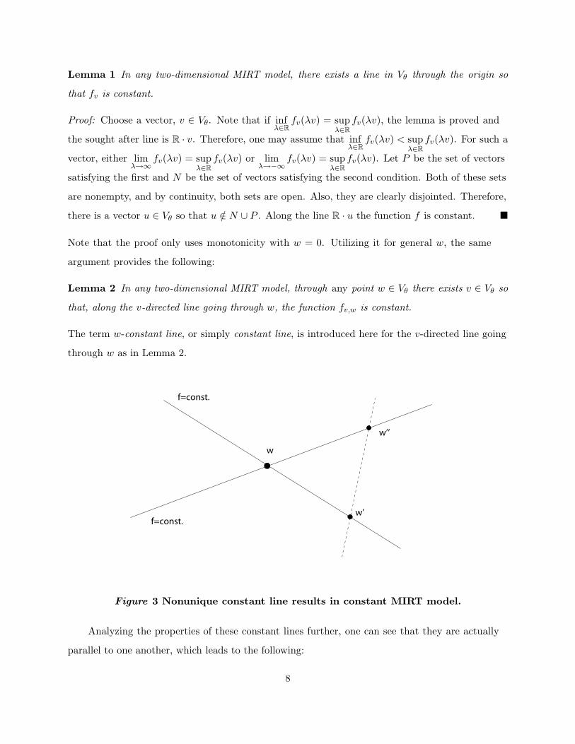
Lemma 2 In any two-dimensional MIRT model, through any point w ∈ Vθ there exists v ∈ Vθ so

that, along the v-directed line going through w, the function fv,w is constant.

The term w-constant line, or simply constant line, is introduced here for the v-directed line going

through w as in Lemma 2.

w

w’’

w’

f=const.

f=const.

Figure 3 Nonunique constant line results in constant MIRT model.

Analyzing the properties of these constant lines further, one can see that they are actually

parallel to one another, which leads to the following:

8

Lemma 3 Let w,w′ ∈ Vθ be two points. Let v, v′ ∈ Vθ be the corresponding directions of the two

constant lines. Then v = µv′ for some µ ∈ R.

Proof: First, note that if there is a point w ∈ Vθ so that there exist two w-constant lines, then the

model is trivial (f is constant) and the statement is true. For, let w′ and w′′ be the intersections

of a general position line in Vθ with the two w-constant lines, respectively. Because f is monotonic

along this line, f(w′) = f(w′′), f is constant between w′ and w′′, that is, f(tw′+(1− t)w′′) = f(w′)

for all t ∈ [0, 1]. Using this argument for every line in a general position proves that f is constant

everywhere (see Figure 3).

Now assume that the constant lines through w and w′ are unique. If the two lines are not

parallel, then they will have an intersection, and an argument similar to the previous one shows

that f is constant. �

The corollary of the previous observation is given in Theorem 1.

Theorem 1 Any two-dimensional MIRT model is a trivial extension of a unidimensional IRT

model.

Proof: Lemma 3 showed that a two-dimensional IRHS is nothing but a collection of parallel lines.

Let v ∈ Vθ be the direction of these lines. By choosing a transversal R · u (a line that intersects

all of them) to this collection, the IRHS can be given by the function fu : R · u→ [0, 1]. One can

express an arbitrary w ∈ Vθ as a unique linear combination w = µu+ λv and write

f(w) = f(µu+ λv) = fu(µu). (12)

This function fu can be thought of as a unidimensional IRT model. �

3.3.2 D-Dimensional Case

Technically, the D-dimensional case is not that much more complicated than the two-

dimensional one. It is just much more difficult to visualize the corresponding geometric objects.

As pointed out earlier, the conditional probability surface is not two-dimensional, so strictly

speaking it is not a surface in higher dimensions. Three-dimensional training does not allow one

to “see” objects in higher dimensions. The formalism built in the previous section, however, is

applicable, with appropriate modifications, to this situation as well.

9

The proof of Lemma 1 works for any dimensions. Applying the monotonicity argument for

arbitrary (v, w) as above proves the corresponding

Lemma 4 In any MIRT model there exists a hyperplane Hw in Vθ through w ∈ Vθ so that fHw is

constant.

Proof: Here, fHw is the restriction of f to the hyperplane Hw. As before, w = 0 is proven explicitly;

the general case follows the same argument. As before, the open sets P and N are denoted, with

P = −N . Exclude the trivial case of P = ∅. It is clear that P ∪N 6= Vθ. Locally the boundary of

P (the closure of P minus P ) is a D − 1 dimensional submanifold (D = dimVθ). Therefore there

exists a collection (c1, . . . , cD−1) of points in Vθ\(P ∪N) so that (c1 − w, . . . , cD−1 − w) spans a

hyperplane Hw. Now, along the line segment joining any point on R · (ci − w) with any point on

R · (cj − w) for some i 6= j, the restriction of f should be constant (Figure 3). Repeating this

argument for each pair of line segments shows that along the entire hyperplane f is constant. If

there is another hyperplane with this property, then P = ∅, which is excluded. �

Now, a D − 1 dimensional hyperplane is to a D-dimensional space as a line is to the plane.

Using this intuition, it is not difficult to adapt the formal proof of Lemma 3 to prove Lemma 5:

Lemma 5 Let w,w′ ∈ Vθ be two points. Let Hw,Hw′ ⊂ Vθ be the corresponding two constant

hyperplanes. Then Hw and Hw′ are parallel.

Now one can rephrase the main theorem in arbitrary dimension.

Theorem 2 Any MIRT model is a trivial extension of a unidimensional IRT model.

For the sake of explicitness, write fM for an arbitrary IRHS in terms of univariate IRT model. A

transversal u ∈ Vθ is fixed to the collection of constant hyperplanes. First, observe that for any

w ∈ Vθ there is a unique decomposition w = µu+ λv with v ∈ Hw. Then

fM (µu+ λv) = fMu (µu). (13)

Note that if the usual 2PL or 3PL models are chosen, the construction yields the scalar

product model. It is also interesting to note that the MIRT generalization of the Rasch model is

equivalent to the generalization of the 2PL model. This is because of the following: while within

the univariate Rasch model, one may assume that the slope is fixed, but when more dimensions

10

are considered simultaneously, the assumption of equal slopes is not valid. The relative positions

of slopes to one another should be determined during the estimation procedure in lack of a priori

information.

This kind of models were called generalized compensatory models (GMIRT) in Zhang and

Stout (1999). The link function of an IRHS as GMIRT is fMu .

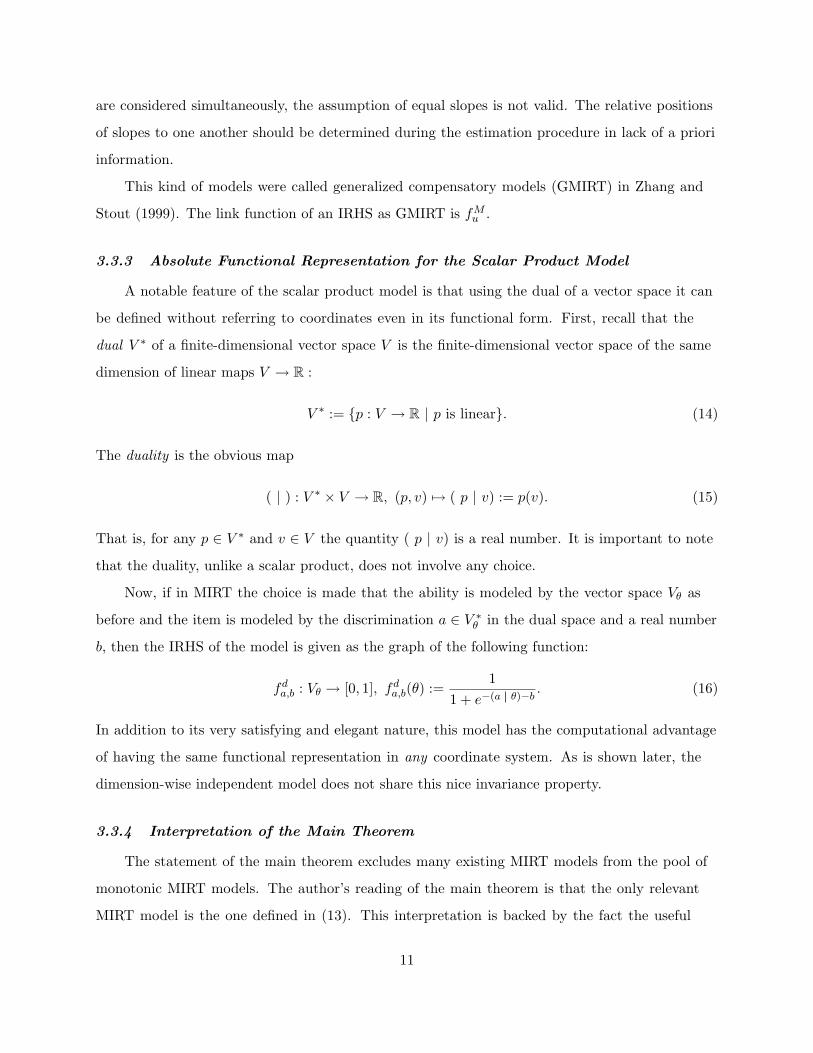
3.3.3 Absolute Functional Representation for the Scalar Product Model

A notable feature of the scalar product model is that using the dual of a vector space it can

be defined without referring to coordinates even in its functional form. First, recall that the

dual V ∗ of a finite-dimensional vector space V is the finite-dimensional vector space of the same

dimension of linear maps V → R :

V ∗ := {p : V → R | p is linear}. (14)

The duality is the obvious map

( | ) : V ∗ × V → R, (p, v) 7→ ( p | v) := p(v). (15)

That is, for any p ∈ V ∗ and v ∈ V the quantity ( p | v) is a real number. It is important to note

that the duality, unlike a scalar product, does not involve any choice.

Now, if in MIRT the choice is made that the ability is modeled by the vector space Vθ as

before and the item is modeled by the discrimination a ∈ V ∗θ in the dual space and a real number

b, then the IRHS of the model is given as the graph of the following function:

fda,b : Vθ → [0, 1], fd

a,b(θ) :=1

1 + e−(a θ)−b. (16)

In addition to its very satisfying and elegant nature, this model has the computational advantage

of having the same functional representation in any coordinate system. As is shown later, the

dimension-wise independent model does not share this nice invariance property.

3.3.4 Interpretation of the Main Theorem

The statement of the main theorem excludes many existing MIRT models from the pool of

monotonic MIRT models. The author’s reading of the main theorem is that the only relevant

MIRT model is the one defined in (13). This interpretation is backed by the fact the useful

11

estimation methods exist only for the scalar product model, the most relevant of the above

extensions (Reckase, 1997). In the view of Theorem 2, there seems to be a good reason behind

that. It seems that lack of monotonicity prevents one from maximizing the likelihood function of

MIRT models excluded by this approach. This certainly defines a valid future research direction.

Also, the existence of an elegant coordinate-free functional representation makes the scalar

product model even more appealing.

On the other hand, model building always has many steps that cannot be entirely backed by

theoretical considerations. The process sometimes is dictated by personal preferences and tastes.

It is possible that some readers may not be willing to accept the requirement of monotonicity

as formulated in Definition 1 as a crucial and necessary feature of an MIRT model. For those

readers the main theorem is interpreted a bit differently. First, note the close connection between

the notion of compensatory model to monotonicity. Usual terminology is that the model is

compensatory if the probability of the correct response may be high even with the lack of ability in

all but one dimension. That is, sufficiently high ability in one dimension is able to compensate for

the lack of it in other dimensions. In fact, compensatory property follows from monotonicity as an

easy application of Theorem 2. If compensatory property is understood in a sense that it is true

in any coordinate system, then the reverse is also true, and the two notions are equivalent. With

this in mind the theorem states that any compensatory MIRT model is a direct generalization of a

univariate IRT model.

In either way, Theorem 2 establishes a prominent role for the scalar product model as an

MIRT model.

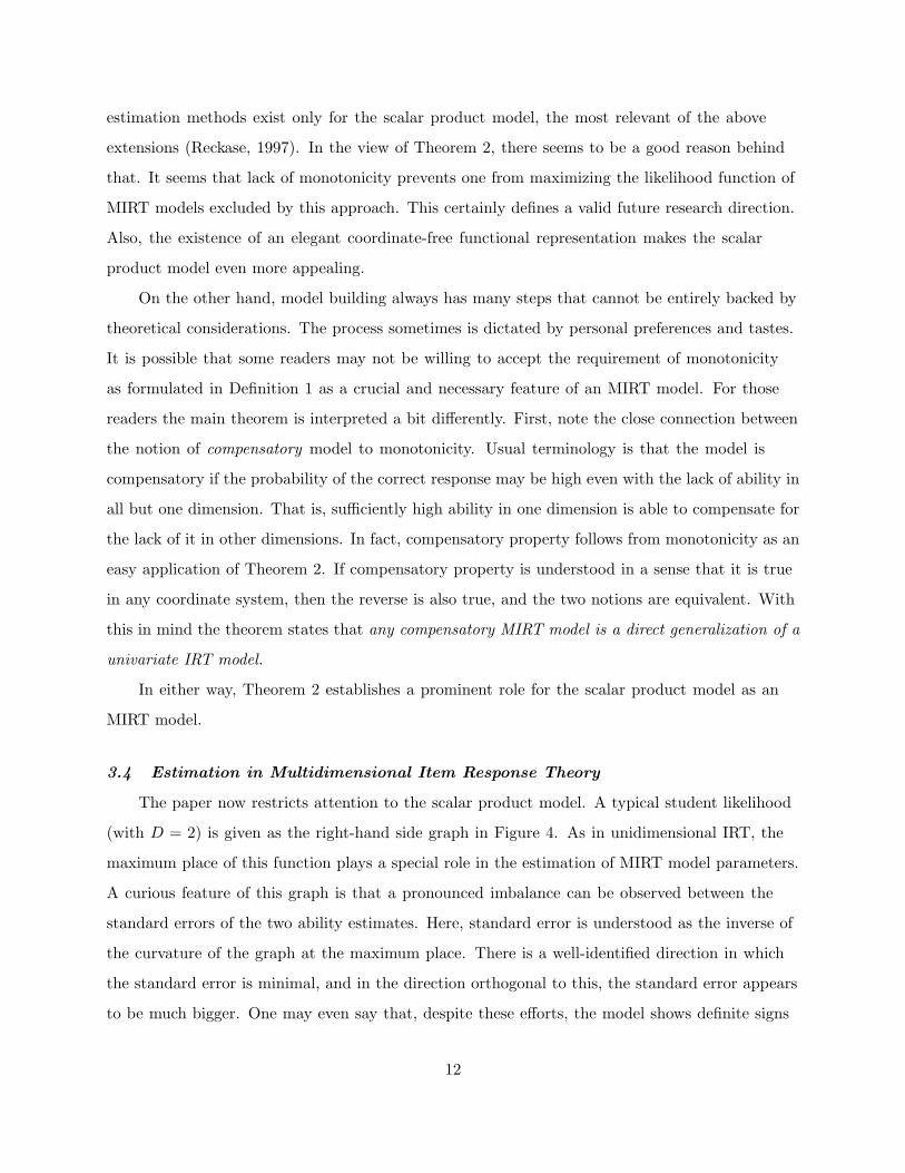
3.4 Estimation in Multidimensional Item Response Theory

The paper now restricts attention to the scalar product model. A typical student likelihood

(with D = 2) is given as the right-hand side graph in Figure 4. As in unidimensional IRT, the

maximum place of this function plays a special role in the estimation of MIRT model parameters.

A curious feature of this graph is that a pronounced imbalance can be observed between the

standard errors of the two ability estimates. Here, standard error is understood as the inverse of

the curvature of the graph at the maximum place. There is a well-identified direction in which

the standard error is minimal, and in the direction orthogonal to this, the standard error appears

to be much bigger. One may even say that, despite these efforts, the model shows definite signs

12

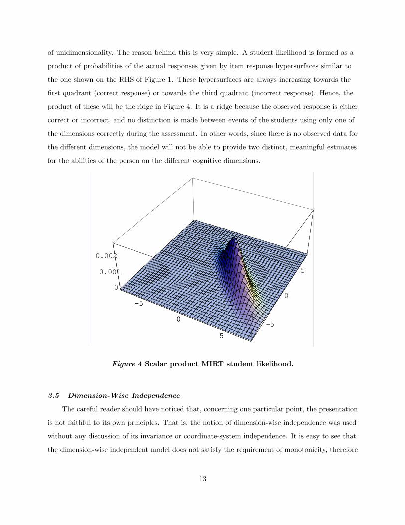
of unidimensionality. The reason behind this is very simple. A student likelihood is formed as a

product of probabilities of the actual responses given by item response hypersurfaces similar to

the one shown on the RHS of Figure 1. These hypersurfaces are always increasing towards the

first quadrant (correct response) or towards the third quadrant (incorrect response). Hence, the

product of these will be the ridge in Figure 4. It is a ridge because the observed response is either

correct or incorrect, and no distinction is made between events of the students using only one of

the dimensions correctly during the assessment. In other words, since there is no observed data for

the different dimensions, the model will not be able to provide two distinct, meaningful estimates

for the abilities of the person on the different cognitive dimensions.

-5

0

5-5

0

5

0

0.001

0.002

-5

0

5

Figure 4 Scalar product MIRT student likelihood.

3.5 Dimension-Wise Independence

The careful reader should have noticed that, concerning one particular point, the presentation

is not faithful to its own principles. That is, the notion of dimension-wise independence was used

without any discussion of its invariance or coordinate-system independence. It is easy to see that

the dimension-wise independent model does not satisfy the requirement of monotonicity, therefore

13

it would not be considered it as a valid MIRT model. On the other hand, it might be useful to see

explicitly how badly the the functional representation of the dimension-wise independent model

behaves and so appreciate the niceties of the scalar product model even more.

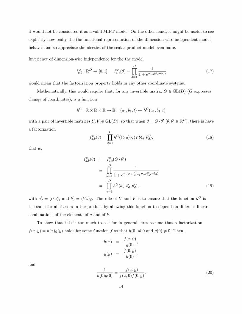
Invariance of dimension-wise independence for the the model

fwa,b : RD → [0, 1], fw

a,b(θ) =D∏

d=1

11 + e−ad(θd−bd)

(17)

would mean that the factorization property holds in any other coordinate systems.

Mathematically, this would require that, for any invertible matrix G ∈ GL(D) (G expresses

change of coordinates), is a function

hG : R× R× R → R, (a1, b1, t) 7→ hG(a1, b1, t)

with a pair of invertible matrices U, V ∈ GL(D), so that when θ = G · θ′ (θ, θ′ ∈ RD), there is have

a factorization

fwa,b(θ) =

D∏d=1

hG((Ua)d, (V b)d, θ′d), (18)

that is,

fwa,b(θ) = fw

a,b(G · θ′)

=D∏

d=1

1

1 + e−ad(PD

d′=1 gdd′θ′d′−bd)

=D∏

d=1

hG(a′d, b′d, θ

′d), (19)

with a′d = (Ua)d and b′d = (V b)d. The role of U and V is to ensure that the function hG is

the same for all factors in the product by allowing this function to depend on different linear

combinations of the elements of a and of b.

To show that this is too much to ask for in general, first assume that a factorization

f(x, y) = h(x)g(y) holds for some function f so that h(0) 6= 0 and g(0) 6= 0. Then,

h(x) =f(x, 0)g(0)

,

g(y) =f(0, y)h(0)

,

and1

h(0)g(0)=

f(x, y)f(x, 0)f(0, y)

. (20)

14

Now, for the sake of concreteness, take D = 2 and a = (a1, a1) ∈ R2 and b = (0, 0) ∈ R2. Also,

take G =

1 1

1 −1

. With these, (19) becomes

11 + e−a1(θ′1+θ′2)

· 11 + e−a1(θ′1−θ′2)

= h(θ′1)g(θ′2) (21)

with some h, g : R → R. From (20) the function

1h(0)g(0)

=1

1+e−a1(θ′1+θ′2)· 1

1+e−a1(θ′1−θ′2)

1

(1+e−a1θ′1 )2· 1

1+e−a1θ′2· 1

1+e+a1θ′2

(22)

should be constant. This is clearly not the case, showing that the factorization (19) does not hold

in general.

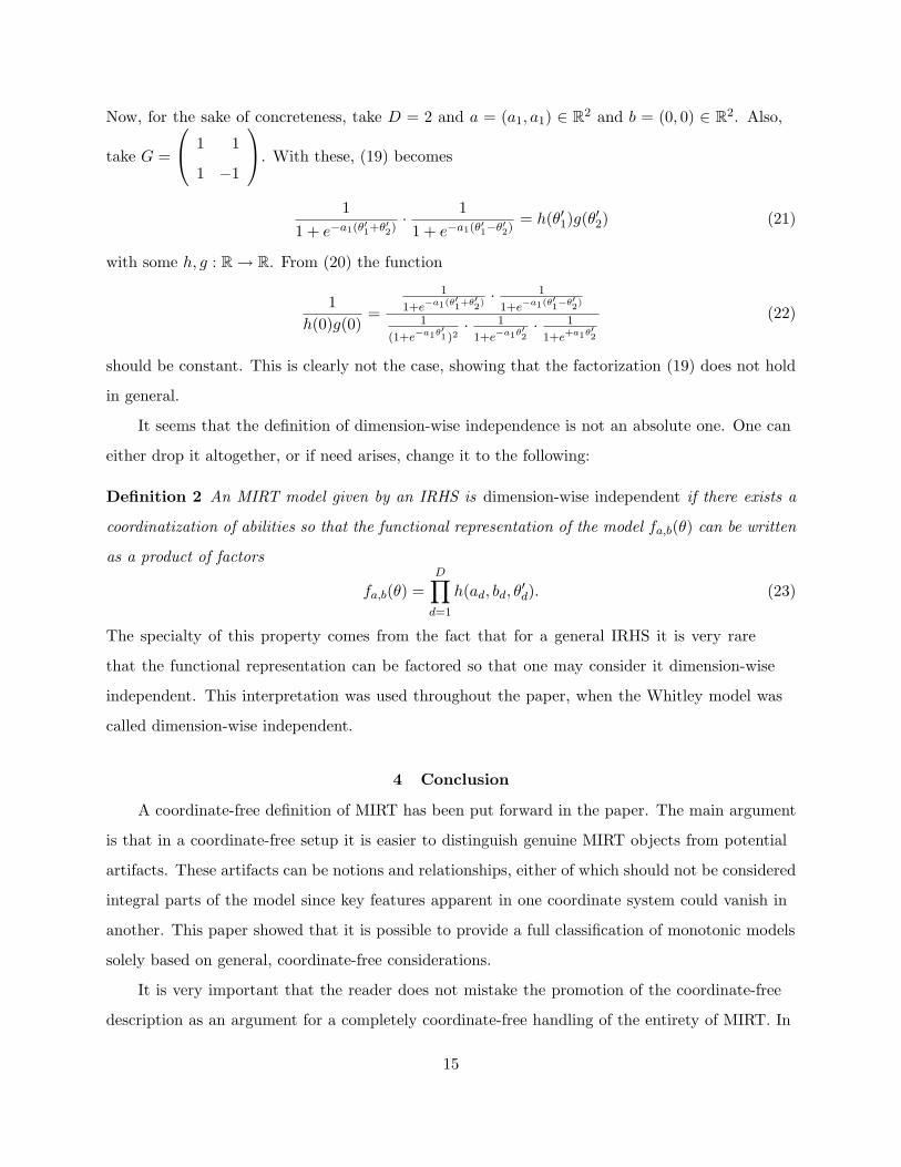
It seems that the definition of dimension-wise independence is not an absolute one. One can

either drop it altogether, or if need arises, change it to the following:

Definition 2 An MIRT model given by an IRHS is dimension-wise independent if there exists a

coordinatization of abilities so that the functional representation of the model fa,b(θ) can be written

as a product of factors

fa,b(θ) =D∏

d=1

h(ad, bd, θ′d). (23)

The specialty of this property comes from the fact that for a general IRHS it is very rare

that the functional representation can be factored so that one may consider it dimension-wise

independent. This interpretation was used throughout the paper, when the Whitley model was

called dimension-wise independent.

4 Conclusion

A coordinate-free definition of MIRT has been put forward in the paper. The main argument

is that in a coordinate-free setup it is easier to distinguish genuine MIRT objects from potential

artifacts. These artifacts can be notions and relationships, either of which should not be considered

integral parts of the model since key features apparent in one coordinate system could vanish in

another. This paper showed that it is possible to provide a full classification of monotonic models

solely based on general, coordinate-free considerations.

It is very important that the reader does not mistake the promotion of the coordinate-free

description as an argument for a completely coordinate-free handling of the entirety of MIRT. In

15

fact, meaningful MIRT practice cannot exist without a choice of coordinates. In addition to this,

every discussion of MIRT features can be fully carried out using RD as the main model space for

abilities. Should such a path be chosen, however, one has to be careful to meticulously maintain

the coordinate-system invariance of the theory every step of the way. The contribution of this

paper is an introduction of a framework to ease this burden by keeping the presentation absolute

(without choosing any coordinates) for as long as possible. The paper shows that one may be

able to formulate general statements and reach valuable insights before switching to relative mode

by an introduction of a particular basis. It is likely that someone may observe the relevance of a

notion while using a particular coordinate system and may want to establish whether the notion

is invariant by trying to create a definition in the absolute framework presented here.

It is noteworthy that the necessity of the existence of a coordinate-free representation of our

physical world led Einstein to formulate both the special and the general theories of relativity

(1905, 1916). The fundamental dogma in relativity theory is that the events of the physical world

take place without there being aware of any coordinate system. Therefore, any faithful description

should be invariant of the change of coordinate system. Better yet, a description of the physical

world is sought that bypasses the use of coordinates altogether.

A reader interested in the successes of coordinate-free description of the physical world may

also find the books by Matalocsi (1986, 1993) useful.

16

References

Birnbaum, A. (1968). Some latent trait models and their use in inferring an examinee’s ability. In

F. M. Lord & M. R. Novick (Eds.), Statistical theories of mental test scores (pp. 397–479).

Reading, MA: MIT Press.

Einstein, A. (1905). Zur elektrodynamik bewegter korper. Annalen der Physik, 17, 891–921.

Einstein, A. (1916). Grundlagen der allgemeinene relativitatstheorie (The foundation of the general

theory of relativity). Annalen der Physik, 49 (4), 284–339.

Halmos, P. R. (1974). Finite-dimensional vector spaces (2nd ed.). New York: Springer-Verlag.

Matolcsi, T. (1986). A concept of mathematical physics: Models in mechanics. Budapest, Hungary:

Akademiai Kiado.

Matolcsi, T. (1993). Spacetime without reference frames. Budapest, Hungary: Akademiai Kiado.

McKinley, R. L., & Reckase, M. D. (1982). The use of the general Rasch model with multidimen-

sional item response data (Research Rep. ONR No. 82-1). Iowa City, IA: ACT.

Reckase, M. D. (1997). A linear logistic multidimensional model for dichotomous item response

data. In W. J. van der Linden & R. K. Hambleton (Eds.), Handbook of modern item response

theory (pp. 271–286). New York: Springer-Verlag.

Warner, F. W. (1971). Foundations of differentiable manifolds and lie groups. Glenview, Illinois:

Scott, Foresman and Company.

Whitely, S. E. (1980). Measuring aptitude processes with multicomponent latent trait models (Tech-

nical Rep. No. NIE-80-5). Lawrence: University of Kansas.

Zhang, J., & Stout, W. F. (1999). Conditional covariance structure of generalized compensatory

multidimensional items. Psychometrika, 64, 129–152.

17