On-line Calibration for Dynamic Traffic Assignment

On–line Calibration for Dynamic TrafficAssignment

Constantinos Antoniou

October 5, 2007

Seminar at Portland State University

Constantinos Antoniou October 5, 2007

Outline

• Introduction

• Formulation

• Solution approaches

• Case study

• Directions for further research

• A glimpse at ongoing research

Seminar at Portland State University 1

!"#$%&'!"#$%&'!"#$%&'!"#$%&'DYnamic Network Assignment

for the Management of Information to Travelers

!"#$%&'!"#$%&'!"#$%&'!"#$%&'!"#$%&'!"#$%&'!"#$%&'!"#$%&' ()*$()*$()*$()*$()*$()*$()*$()*$

)(+, $.(/#01$)23

42$ 0.(+2*)").2+

5423(6.(#7*.4$88(6

54/9(3(#7*.4$92 *(#8/4+$.(/#

DynaMIT GUI

:(+, $.(/#:(+, $.(/#:(+, $.(/#:(+, $.(/#:(+, $.(/#:(+, $.(/#:(+, $.(/#:(+, $.(/#

!!2+$#3; %(64/*)(+, $./4; !25$4.,42*.(+2*6</(62; =/,.2*6</(62; =2)5/#)2*./*&':; >4(7(#032).(#$.(/#*8 /?)

!:,55 "; %2)/)6/5(6 '4$88(6*)(+, $./4

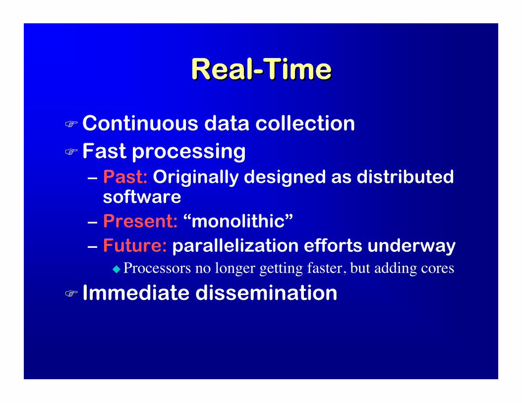
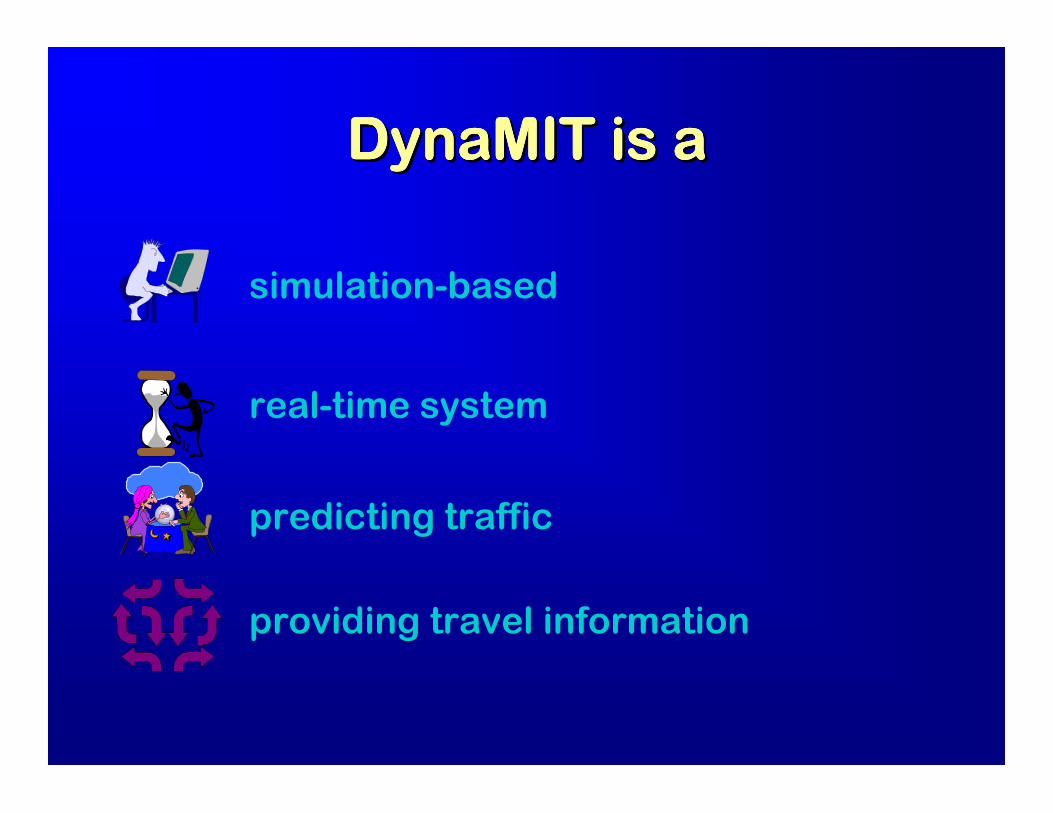
=2$ =2$ =2$ =2$ =2$ =2$ =2$ =2$ 00000000'(+2'(+2'(+2'(+2'(+2'(+2'(+2'(+2

!@/#.(#,/,)*3$.$*6/ 26.(/#!A$).*54/62))(#7

; B$).C >4(7(#$ "*32)(7#23*$)*3().4(1,.23*)/8.?$42

; B42)2#.C D+/#/ (.<(6E; A,.,42C 5$4$ 2 (F$.(/#*288/4.)*,#324?$"

"Processors no longer getting faster, but adding cores

! &++23($.2*3())2+(#$.(/#

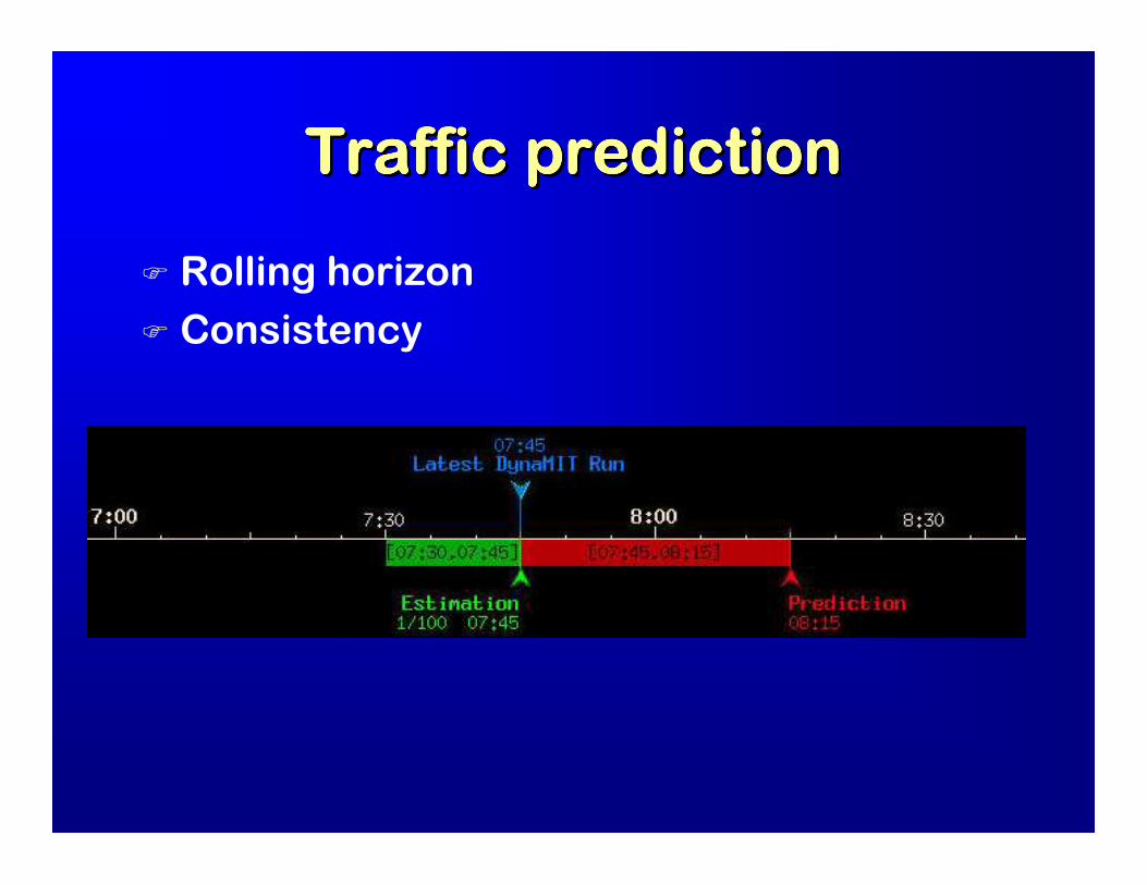
'4$88(6*5423(6.(/#'4$88(6*5423(6.(/#'4$88(6*5423(6.(/#'4$88(6*5423(6.(/#'4$88(6*5423(6.(/#'4$88(6*5423(6.(/#'4$88(6*5423(6.(/#'4$88(6*5423(6.(/#

! =/ (#7*</4(F/#! @/#)().2#6"

=/ (#7*G/4(F/#=/ (#7*G/4(F/#=/ (#7*G/4(F/#=/ (#7*G/4(F/#=/ (#7*G/4(F/#=/ (#7*G/4(F/#=/ (#7*G/4(F/#=/ (#7*G/4(F/#

!"#$%&'!"#$%&'!"#$%&'!"#$%&'!"#$%&'!"#$%&'!"#$%&'!"#$%&' 6/#).$#. "*5423(6.)*.4$88(6*6/#).$#. "*5423(6.)*.4$88(6*6/#).$#. "*5423(6.)*.4$88(6*6/#).$#. "*5423(6.)*.4$88(6*6/#).$#. "*5423(6.)*.4$88(6*6/#).$#. "*5423(6.)*.4$88(6*6/#).$#. "*5423(6.)*.4$88(6*6/#).$#. "*5423(6.)*.4$88(6*6/#3(.(/#)*8/4*$*5426/#3(.(/#)*8/4*$*5426/#3(.(/#)*8/4*$*5426/#3(.(/#)*8/4*$*5426/#3(.(/#)*8/4*$*5426/#3(.(/#)*8/4*$*5426/#3(.(/#)*8/4*$*5426/#3(.(/#)*8/4*$*54200000000)526(8(23*.(+2*524(/3)526(8(23*.(+2*524(/3)526(8(23*.(+2*524(/3)526(8(23*.(+2*524(/3)526(8(23*.(+2*524(/3)526(8(23*.(+2*524(/3)526(8(23*.(+2*524(/3)526(8(23*.(+2*524(/3

8:007:55 9:00

Estimation PredictionRunning

time

8:007:55 9:00

Estimation PredictionRunning

time

8:07

8:07

9:07

At 8:00

At 8:07

Broadcasting forecasts does not affect the weather

But with traffic…

DynaMIT Evaluation

MITSIM

Surveillance System

DynaMIT

Information

%2$),42)/8

28826.(92#2))

!"#$%&'!"#$%&'C*H2.?/4I*=2542)2#.$.(/#C*H2.?/4I*=2542)2#.$.(/#

!"#$%&'!"#$%&'

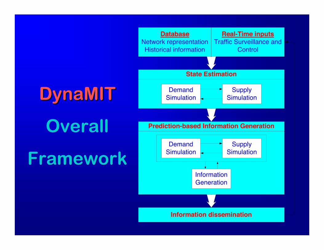
>924$

A4$+2?/4I

Information dissemination

DatabaseNetwork representationHistorical information

Real-Time inputsTraffic Surveillance and

Control

State Estimation

DemandSimulation

SupplySimulation

Prediction-based Information Generation

InformationGeneration

DemandSimulation

SupplySimulation


On–line DTA framework

Demand

simulator

Supply simulator

State estimation and model calibration

Network representation

Historical data

A-priori

parameter

values

Surveillance

information

Demand

simulator

Supply simulator

State prediction

Network

performance



Motivation• Models/components

– Demand–side! OD flows! Behavioral models (e.g. route choice)

– Supply–side

! Speed–density relationship (e.g. u = uf

[1 !

(max(0,K!Kmin)

Kjam

)!]"

· where u denotes the speed, uf is the free flow speed, K is thedensity, Kmin is the minimum density, Kjam is the jam density and" and ! are model parameters.)

! Segment capacities

• Existing state estimation and model calibration approaches include subsetof these models



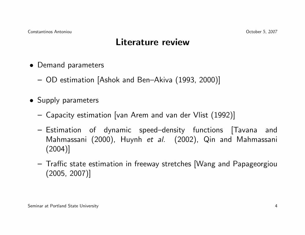
Literature review

• Demand parameters

– OD estimation [Ashok and Ben–Akiva (1993, 2000)]

• Supply parameters

– Capacity estimation [van Arem and van der Vlist (1992)]

– Estimation of dynamic speed–density functions [Tavana andMahmassani (2000), Huynh et al. (2002), Qin and Mahmassani(2004)]

– Tra!c state estimation in freeway stretches [Wang and Papageorgiou(2005, 2007)]



Research objectives

• Develop an integrated approach for on–line calibration that

– Jointly estimates and predicts demand and supply parameters

– Is general and flexible! Not tied to a particular DTA system

! Applicable to any calibration parameters

! Can exploit any available information

– Is computationally feasible

• Demonstrate the feasibility of the approach



Inputs and outputs

On-line

calibration

A priori

parameter

values

Surveillance

data

Historical

data

On-line calibrated

parameters



Formulation

• State–space model

– State vector

– Measurement equations

– Transition equations

• Idea of deviations



State vector

• Deviations #!h of model inputs and parameters !h from availableestimates

#!h = !h ! !Hh

• State vector includes

– OD flows xijh: number of vehicles departing from origin i towardsdestination j during time interval h

– Model parameters, e.g.! route choice model parameters

! speed–density relationship parameters

! segment capacities



Measurement equations (I)

• Direct measurement equation

!ah = !h + vh

• In deviations’ form (subtracting !Hh from both sides)

!ah ! !H

h = !h ! !Hh + vh !

#!ah = #!h + vh

where

– a denotes a priori values, H indicates historical estimates, vh is arandom error vector.



Measurement equations (II)• Indirect measurement equation

Mh = S(!h

)+ "h

• In deviations’ form (subtracting MHh from both sides)

Mh ! MHh = S

(!h

)! MH

h + "h !

#Mh = S(!H

h + #!h

)! MH

h + "h

where

– Mh is a vector of measurements for interval h, and "h is a randomerror vector.

– S is the simulator function mapping the state to the measurements(no analytic expression).



Transition equations

!h+1 =h"

q=h!p

Fh+1q · !q + #h

• In deviations’ form (subtracting !H for appropriate interval from bothsides)

!h+1 ! !Hh+1 =

h"

q=h!p

Fh+1q

(!q ! !H

q

)+ #h !

#!h+1 =h"

q=h!p

Fh+1q · #!q + #h

where

– Fh+1q is a transition matrix of e"ects of #!q on #!h+1

– p is the degree of the autoregressive process, and– #h is a random error vector



The model at a glance

#!ah = #!h + vh

#Mh = S(!H

h + #!h

)! MH

h + "h

#!h+1 =h"

q=h!p

Fh+1q · #!q + #h



Solution approaches

• Linear models

– Kalman Filter (KF)

• Non–linear models

– Extended Kalman Filter (EKF)– Limiting Extended Kalman Filter (LimEKF)– Unscented Kalman Filter (UKF)



Kalman Filtering principles

• Prediction–correction approach

1. Predict a priori state for interval h (using information up to h ! 1)

2. Compute Kalman gain matrix

3. Combine Kalman gain and surveillance from interval h to correct stateprediction for interval h



Extended Kalman Filter

• Extension of Kalman Filter for non–linear models

– First order Taylor expansion approximation

• Can use numerical derivatives, if no analytical relationship exists (formeasurement equations)

– Large number of function evaluations is required– e.g. 2n evaluations if central di"erences are used (n is state dimension)

• Computation of Kalman gain most “expensive” operation



Limiting Extended Kalman Filter

• Use a pre–computed Kalman gain

– E.g.: (weighted) average of Kalman gains (computed o"–line)– No need to compute the Kalman gain on–line

• Only a single function evaluation is required on–line

• Can run EKF o"–line and periodically re–compute Kalman gain



Unscented Kalman Filter

• Uses Unscented Transformation

– The state mean and covariance are used to generate 2n + 1 sigmapoints (n is the dimension of the state)

– These points are propagated through the true nonlinearity

• Kalman gain is computed from the state and measurement covariances

• No limiting version is possible

– Mean measurement vector (from 2n + 1 replications) is required forthe correction stage



Case study — Objectives

• Demonstrate feasibility of the on–line calibration approach

• Verify importance of on–line calibration

– Impact of joint estimation and prediction of demand and supplyparameters

• Test candidate algorithms based on several criteria

– Performance/Fit (estimation and prediction)– Computational properties– Robustness



The DynaMIT–R system

• State–of–the–art, simulation–based DTA system

– Transportation network and supply characteristics– OD demand and travel behavior

• Operates in rolling horizon for:

– Real–time estimation of network performance– Short–term prediction of future network conditions– Generation of tra!c information

• Inputs

– A-priori OD flows– Route choice parameters– Tra!c dynamics models’ parameters– Segment capacities



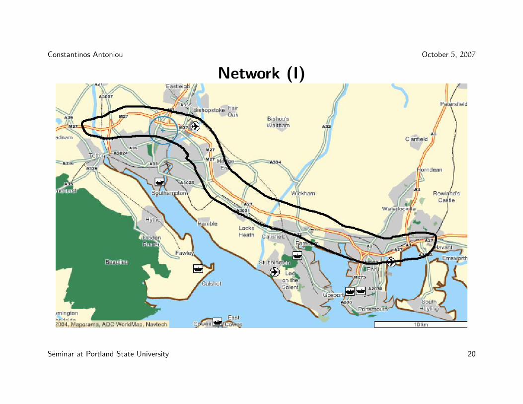
Network (I)



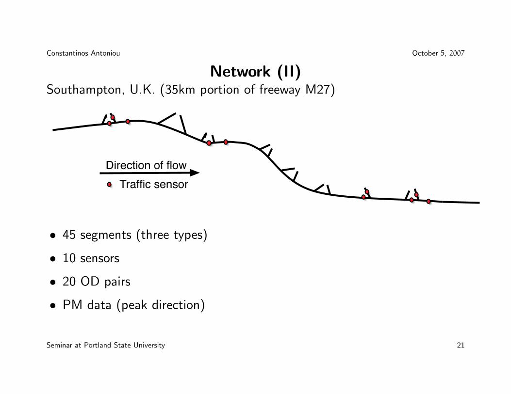
Network (II)Southampton, U.K. (35km portion of freeway M27)

Direction of flow

Traffic sensor

• 45 segments (three types)

• 10 sensors

• 20 OD pairs

• PM data (peak direction)



Traffic flow characteristics



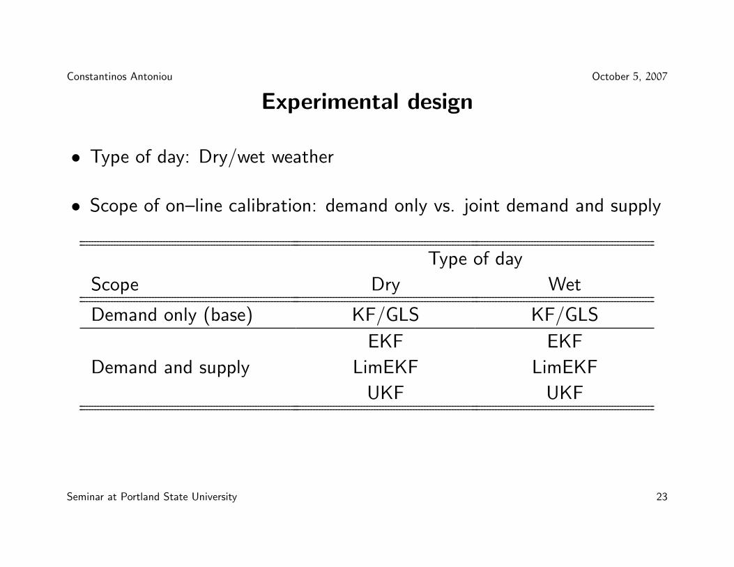
Experimental design

• Type of day: Dry/wet weather

• Scope of on–line calibration: demand only vs. joint demand and supply

Type of day

Scope Dry Wet

Demand only (base) KF/GLS KF/GLS

EKF EKF

Demand and supply LimEKF LimEKF

UKF UKF



Measures of effectiveness

1. Fit of estimated/predicted vs. observed speeds

2. Fit of estimated/predicted vs. observed sensor counts

• Aggregate statistic: Normalized root mean square error (RMSN)

RMSN =

√N"

#n=1:N(yn ! yn)2

#n=1:N yn

3. Computational performance



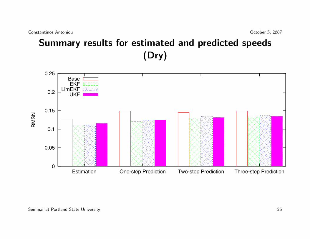
Summary results for estimated and predicted speeds(Dry)

0

0.05

0.1

0.15

0.2

0.25

Three-step PredictionTwo-step PredictionOne-step PredictionEstimation

RMSN

BaseEKF

LimEKFUKF



Summary results for estimated and predicted speeds(Wet)

0

0.05

0.1

0.15

0.2

0.25

Three-step PredictionTwo-step PredictionOne-step PredictionEstimation

RMSN

BaseEKF

LimEKFUKF



On–line calibrated speed–density relationshipsMainline segments – EKF

top: dry weather, bottom: wet weather

10 20 30 40 50 60

70

80

90

10

01

10

12

0

Density (veh/km/lane)

Sp

ee

d (

kp

h)

!

!

!

!!

!

!

!

!

!

!

!

!

!

!

!

!

!

!

!

! !

!

!

!

!

!

!

!

!!

!

!

!!

!

!

!!

!

!!

!

!

!! !

!

!

!

!!

!!

!

!

!!

!

!

!

!

!

!

!

!

! !

!

!

!

!

!

!

!!

!

!

!

!

!

!

!

!

!

!

!

! !

!

!

!!

!!

!

!

!

!

!

!

!

!!

!!

!

!!

!

!

!

!

!

!

!

!

!

!!

!

!

!

!

!

!!!

!

!

!

!

!

!

!

!

!

!

!

!

!

!!

!

!

!

!

!

!

!

!

!!

!

!

! !

!

! !

!

!

!

!

!

!

!!

!

!

!

!

!

!

!

!

!

!

!

!

!

!

!

!

!

!

!!

!

!

!

!

!!

!

!!

!

!

!!

!!

!

!

!

!

!

!

! !

!

!

! !!

!!

!

!

!

!

!

!!!

!

!

!

!

!

!

! !

!

!

!

!

!!

!

!

!

!!

!

!

!

!

!

!!

!!

!

!!

!

!

!!!

!

!

!

!

! !

!

!

Off!lineOn!line

! Observations

10 20 30 40 50 60

70

80

90

10

01

10

12

0

Density (veh/km/lane)

Sp

ee

d (

kp

h)

!

!

!

!

!

!

!

!!

!

!

!

!

!

!

!

! !

!

!!

!

!

!!

!

!

!

!

!

!

!!

!

!

!

!

!

!

!

!

!

!!

!

!

!

!!

!

!

!

!

!

!!

!

!

!

!

!

!

!

!

!

!

!

!

!

!

!

!

!

!

!

!

!!

!

!

!

!

!

!

!

! ! !

!

!

!

!!!

!

!!

!

!

!

!

!

!

!

!!!

!

!

!

!!

!!

!!

!

!

!

!

!

!

!

!!

!

!

! !

!

!

!

!

!

!!

!

!

!

!

!

! !!

!

!

!

!

!

!

!

!! !

!

!

!

!

!

!

!

!

!

!

!!

!

!

!

!

!

!

!

!

! !

!

!

!

!

! !

!

!

!

!

!

!

!!

!!

!

!

!

!

!

!

!

!

!

!

!!

!

!

!

!

!

!

!

!

!

!

!!

!

!

!

!

!

!!

!

!

!

!

!

!

!

! !

!

!

!!

!

!

! !

!

!

!!!

!!

!

!

!

!

!!

!

!

!

!!

!!

!

!

!!

!

!

Off!lineOn!line

! Observations



Computational performance (I)

• EKF/UKF

– Similar performance (2n vs. 2n + 1 function evaluations)

• Limiting Kalman Filter

– Order–of–magnitude improvement

– Single function evaluation required (independent of state dimension)



Computational performance (II)

Function Runtime

evaluations (min:sec)

EKF 2n 98:29

LimEKF 1 0:43

UKF 2n 97:44

• Pentium 4 2.8GHz computer with 512MB RAM



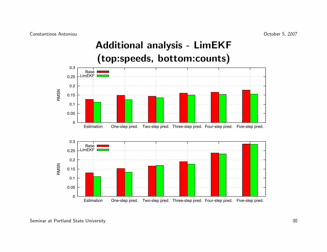
Additional analysis - LimEKF(top:speeds, bottom:counts)

0

0.05

0.1

0.15

0.2

0.25

0.3

Five-step pred.Four-step pred.Three-step pred.Two-step pred.One-step pred.Estimation

RMSN

BaseLimEKF

0

0.05

0.1

0.15

0.2

0.25

0.3

Five-step pred.Four-step pred.Three-step pred.Two-step pred.One-step pred.Estimation

RMSN

BaseLimEKF



Conclusions/Findings (I)

• Joint on–line calibration of demand and supply parameters can improveprediction accuracy

• Changes in parameters are consistent with tra!c engineering principlesand expectations

• Interactions between many parameters are captured

– Many degrees of freedom



Conclusions/Findings (II)

• EKF/UKF: “Real-time” performance in a small, but non-trivial realnetwork

• Limiting EKF

– Order(s) of magnitude improvement in computational performance

– Comparable accuracy to EKF/UKF

– Robustness



Conclusions/Findings (III)

• EKF has more desirable properties than UKF (in this application)

– EKF generally outperforms UKF! Full power of UKF is not exhibited, because transition equation is

already linear

– UKF is not as robust (perhaps due to the number of points used)

– EKF and UKF have similar computational properties

– Limiting EKF (while no similar UKF version exists)



Directions for further research

• Further experimental analysis

– Scalability– Robustness– Sensitivity

• Impact of grouping segments (for speed–density relationship estimation)

• Algorithms

– e.g. particle filters (generalization of UKF)



A glimpse at ongoing researchMesoscopic traffic simulation

Density

Calculate speed

Advance vehicles

Data-

base

Density and other

explanatory variables

Calculate speed

Advance vehicles

Typical approach Alternative approach

u=f(k)



More flexible functional forms

Plus: easily incorporate additional measurements



A comparison of data–driven approaches (I)

• Locally weighted regression

• Support vector regression

• Neural networks



A comparison of data–driven approaches (II)



A comparison of data–driven approaches (III)

Notes: Application runtimes. SVR is an order of magnitude slower.



An integrated machine learning approach

k-means,

Fuzzy c-means, etc

Flexible

relationships f(x)

K-nearest

neighbors

Clustering

Fitting

Classification

Flexible

relationships f(x)Estimation

Training data

(Speeds/Densities/flows)

Estimated

speeds

Training

Explanatory data

(Densities/flows)

Application



An integrated approach: loess and clustering (I)

!!

!

!

!

!

!!

!

!

!

!!

!

!

!

!

!

!

!

!

!!

!

!

!

!

!

!

!

!!

!!

!!

!!

!

!!

!!

!

!

!

!!

!

!

!

!

!

!

!

!!

!

!!

!!

!

!!!

!

!

!

!

!

!

!!

!

!!

!

!!!

!

!

!

!!!

!

!

!

!!

!!

!

!

!!

!!

!

!

!!!!

Classic

loess

(dsy)

loess

(dsy+flw)

loess!clust

(dsy)

loess!clust

(dsy+flw)

!40

!20

020

40

B. Distribution of speed deviations by approach

Approach

Devia

tions in s

peeds (

kph)



An integrated approach: loess and clustering (II)

!!!!! !!!! !! !!!!! ! !! !! !!! ! !!! !!!!!! !! ! !! !! !! !!!! !! !!! !!! ! !!!! ! ! !! ! ! !!!! !!!!! !!!! ! !!!! ! !! !! !! ! ! !!! ! !!! !! !! ! !!!! !!! !! !!!!!! !! ! !!! !!! !!! !!! !!!!! !!! !! !!!!!! ! !!!!! ! ! !!! ! !! ! !! !!!!! ! !! !! !! !!! !! ! !!!!! !!! ! ! !! !!!! !!! !! !! ! ! !! ! ! !!!! !! !!!!!!! !! !! !! ! !!!!! !!!!!!! !!! !!!!!! !! ! ! !!! !!! !! !! ! !!!! ! !!! !!!

!

!! !! !!! !! !!! !!!! !!!! !! ! !!!!

!!! !!!!!!! !!! !!! !!

!!

!

!! !!

!

!!

!

!!!

!!!

! !!

!!!! !!! !

!!!

!

!!!

!

!!!

!! !

!

!!!! !!! !!!!!

!

!!

!

!

!!!

!

! !

!

! !

!

!!!!

!

!!

!

!!

!

!!!!!

!!

!

!! !!

!!

!!

!

!!

!

!!

!

!!

!

!!

!

!!!!

!

!! !!

!!

!

!!!!

!

!!

!

!!

!

!

!

!

!

!!

!

!

!

!

!!

!!!

!

!

!

!

!

!

!!!

! !

!

!

!!

!

!

!

!

!

!

!

!!

! !!

!

!

!!!!

!

!!!

!!!

!!

!!

!!!

!!

!

!!!

!!!

!!

!

!

!

!

!

!!! !

!!

!! !

!!!

!!

!

!

!

!

!!

!!

!!!

! !! !

!! !

!! !!

!!!

!

!!

!

!

!!

!!

!

!!!

!

!

!!

!

!

!!

!!

!

!!!!!

!

!!!!

!!

!!

! !!! !!!

!!

!

!!!!! !! !!! !! !! !!! ! !!!! !! !!!!! !!! !!! !!!!! !!!!!! !! !!!!!

!!! !!! !! !!!! !! !!!! ! !!! ! !!!! !! !!!!!!!!! !! !

0 50 100 150

050

100

150

A. Classic speed!density relationship

Observed speeds(kph)

Estim

ate

d s

peeds (

kph)

!!!!! !!!! !! !!!!! ! !! !! !!! ! !!! !!!!!! !! ! !! !! !! !!!! !! !!! !!! ! !!!! ! ! !! ! ! !!!! !!!!! !!!! ! !!!! ! !! !! !! ! ! !!! ! !!! !! !! ! !!!! !!! !! !!!!!! !! ! !!! !!! !!! !!! !!!!! !!! !! !!!!!! ! !!!!! ! ! !!! ! !! ! !! !!!!! ! !! !! !! !!! !! ! !!!!!

!!! ! ! !! !!!! !!!!! !! ! ! !! ! ! !!!! !! !

!!!!!! !! !! !

!!

!!!!! !!!!

!!

! !!! !!!!!!

!! ! ! !!! !!! !! !

! !!!

!! ! !!! !!

!

!

!! !!

!!!

!! !!! !!!! !!!! !! ! !!!

!!!

! !!!

!!!!!!

!!!

! !!!

!

!

!! !!

!!!!

!!!

!!!

! !!

!!!

!!!!

!!!!

!

!!!

!!!

!!! !

!

!!!! !!! !!!!!

!

!!

!!

!!

!

!

! !

!! !

!

!!!!

!

!!!

!!!

!!!!!

!!

!

!! !

!!!

!!

!

!!

!

!!

!

!

!!

!!

!

!!!!

!

!! !!

!!

!

!!!!

!

!!

!

!!

!

!

!

! !

!! !

!

!

!

!

!

!!!

!

!

!

!

!

!

!!!

! !

!

!

!!

!

!

!

!

!

!

!!

!

! !!

!

!

!!!!

!

!!!

!!!

!!

!!

!

!!

!!

!

!!!

!

!!!!

!

!

!

!

!

!!! !

!!

!! ! !!!

!!!

!

!

!

!!

!

!

!!!

! !! !

!! !

!! !!

!!!

!

!!

!

!!

!

!!

!

!!!

!

!

!!

!

!

!!

!!

!! !!!!

!

!! !!!

!

!!

! !!

! !!!

!!

!

!!!!! !!

!!

!!! !! !!! ! !!

!! !! !!!

!! !!

! !!!

!!!!! !!!!!

!!! !

!!!!

!!!!

!! !! !!!!

!! !!

!! ! !!! ! !!!! !! !!!!!!!!! !! !

0 50 100 150

050

100

150

B. Loess (density)

Observed speeds (kph)

Estim

ate

d s

peeds (

kph)

!!!!

!

!!

!!

!

!

!!

!!

!!

!!

!!!

!!

!!

!!

!

!!!

!! !! !

!

! !

! !

!!

!!

!

!

!

!!!

!!!

!

!

!

!

!!

! !

!

!

!!!

!

!

!

!!

!!

!

!!

!

! !!

!!

!!!

!

!

!

! !

!!

!

!

!

!

!!

!

!

!! ! !!

!

! !

!

!

!

!

!!!

!!

!

!

!

!!

!!

!!!

!!

!

!!

!

!!!!! !

!

!

!!

!!

!!!

!

!

!!

!

!

!

!

! !!

!

!

!

!

! !!

!

!!!

!!

!

!

!

!

!!

!

!

!

!

!!

!!!

!!

!!

!

!!

!!

!

!

!!

!

!! !

!

!!

! !

!

!

!

!!!

!

!

!

!!!!

!!

!

!

!

!

!

!

!

!

!!!

!!

!

!

!!! !!!

!

!!

!!!

!

!!

!

!!

! !

!!

!!!

!

! !

!

!!

!

!!!

!!!

!!!

!

!

!

!!

!!! !!

!!

!!

!!

!

!!!! !

!

! !!!

! !!

!

!!!

!!!!

!!

! !!

!

!

!!

!

!

!!!

!!

!!!

!!!!!!!

!

!!! !

!!!

!!

!!!!!!!

!

!!

!!

! !!

!!

!!!!!

!!!!

!

!

! !!!!

!

!!! !

!!

!!!!!!

!!!!

!!

!!!

!!!

!

!!!!!

! !!

!

!

!

!

!!

!

!

!!

!

!!

!! !!!!!!

!!!

!!!!!

!!!!!

!!

!!

!

!

!

!

!! !!

!

!

!!!!!!

!

!! !

!

!

!!!

!!!! !

!!

!

!

!

!!

!

!

!

!!!

!

!!!!!!

!!!!!

!

!!!

!!!

!!

!

!!!

!

!!!!

!

!!

!

!

!!

! !!!

!!

!

!!

!!!!

!!

!!!!

!!

!!

!

!!!

!!

!!! !!!!!

!

!!

!!

!!!

!

!

!!!

!

!!!

!

!

!!

!

!!

!

!!!

! !

!! !!

!

!!!

!!

!!

!

!

! !!!

!!!!!

!!

!

!

!

!

! !!

!

!

!

!!!

!! !

!!!!!

! !!

!!!

! !!

!

!!!

!!!!!!! !

!

!!!

!!!

!!!

!! !!!

!

!

!

!!!

!

!!

!! !!

!!!

!

!

!!!

!

!!

!!! !

!

!

0 50 100 150

050

100

150

C. Loess (density+flow)


Estim

ate

d s

peeds (

kph)

!!!!

!!

!!!

!

!

!!!!!

! !!!

!!

!

!

!

!!

! !!

!!

!! !!!

!

!!

! !! !!!

!

!

!!!!

!!! !

!

!

!

!!

!!!

!

!!!

!!

!

!

!

!!

!

!!

!

!

!!

!

!

! !!

!

!!

!

!

! !

!!!

!!!

!

!

!!!

!!

!

! !

!!

!!

!!

!

!

!

!

!

!

! !!! !!

!

!!

!

!!

!

!!

!

!

!!!

!

!!!

!

!!!

!

! !!!

!

!

! ! !!!

!

!!

! !! !!!!

! !

!

!

!

!

!

!

!!

!

!

! !!!!!!

!!

!

! ! !

!

!!

!!

!!!

!! !!

!!

!!

! ! !!!!

!

! !!!!!!

!

!

!!

! !

!

!!!

!!!

!!

!!!!

!

!

!!

!!!!

!!

!

!

!

! !

!!

!!!

!

! !

!

!!!

!!

! !!!

!!!

!

!

!!! !!

!!!!!

!

!!!

!!!!

! !!

! !!!

! !!

!!!

!

!!

!!

!

!

!!

!

!!

!!!

!!!

!!! !!!

!!!!!!! !

!!! !

! !!

!!

!!!!

!!!!

!!

!!

!!

!!

!!!!!!

!!!!!

!

!!

!!

!!!!

! !

!! !!

!!!

!

!!!!!!

!

!

!!!

!

!

!!!

!!

!!!

!!

!

!

!

!

!

!!

!

!

!!

!!

!!!!

!!!

!!

!! !

!!

!!

!!!

!

!!!

!

!

! !

!! !!

!

!!!

!!!!

!

!

!

!

!

!

!!! !

!!! !

!!

!

!

!

!

!

!!

!

!!!

!

!!!

!

!

!

!!!!!

!

!!!

!!

!!!

!!!

!!

!!!!

!

!!

!

!

!!! !

!!

!! !

!!

!!!!

!!!

!!!

!!

!!

!!! !

!!

!!! !!!!

!!

!!!

!!!!

!

!

!!!

!

!

!!

!

! !!

!

!!

! !!!

!

!

!! !!

!!!!

!!

!!

!

!

!

!!

!!!!!

!

!

!!

!

!

!

!!

!

!!

!

! !!!!!

! !!!!! !

!!!!!!!

!!!

!!

!

!!

!!!!

!

!!!

!!! !

!!

!! !!!

!!

!!

!!

!

!

!!! !

!

!

!!

!

!

!!!!!

!!!

! !

!!

0 50 100 150

050

100

150

D. Clustered Loess (density)


Estim

ate

d s

peeds (

kph)

!!!!

!

!!

!! !

!

!!

!

!

!

!

!

!

!!

!

!

!

!

!

!

!

!

!!!!!

!!

!

!

!!

!

!

!

!

!!

!

!

!

!!!

!!

!

!!

!

!

! !

!!

!!

! !!

!!

!!!

!!

!!!

!

! !!

!

!

!!!

!

!

!

!!

!

!!

!

!

!

!!

!

!

!! !!

!

!

!

!

!!

!

!

!!!!!

!

!

!

! !

!

!!

!

!

!!

!

!!

!!!

!!! !!

!

!!!

!!

!!

!

!

!!

!

!

!

!! !!

!

!

!

!

! !!

!

!!!

! !

!

!

!

!

!!

!

!

!

!

!! !!

!

!!

!!

!

! ! !!

!!

!!

!

!!

!

!!!

!! !

!

!

!!

!!

!!

! !!!!!!

!

!

!!

! !

!

! !!!!!

!!!! !!!

!

!!

!!!

!!!

!

!

!

! !

!!

!!

!

!

! !

!

!!!

!!! !

!!!!!

!

!

!

!

!

!!! !!

!!

!

!

!!!

!!!! !

!

! !!!

! !!

!

!!!

!!!!

!!

! !!

!!

!!!

!

!!!

!!

!!

!

!!!!!!

! !

!!! !

!!!

!!

!!!!!!!

!

!!

!!

! !!

!!

!!!!! !

!!!!

!

! !!!!

!

!!

! !

!!

!!!!!!

!!!!

!!

!

!!!!

!

!

!!!!!

! !!

!

!

!

!

!

!

!

!

!!

!!!

!!!!

!!

!!!!!

!! !!!

!!!!!

!!

!!

!

!

!

!

!! !

!

!!

!!

!!!!

!

!

!

!

!

!

!!!

!

!!! !

!!!

!

!

!

!!

!

!

!!!

!

!!!!

!!!!!!!

!

!!!

!!!

!!

!!!!!

!!!!

!

!!

!

!

!!! !!

!

!!

!!!

!!!!

!!!

!!!

!!

!!

!

!!!

!!

! !! !!!!!

!

!!

!!

!!!

!

!

!!!

!

!

!

!

!

!

!!

!!!

!!

!!

! !

!! !!

!

!!!

! !!

!

!

!

! !!

!

!!!!!!!

!

!

!

!

!!

!

!!

!!

!!

!!!

!!!!!

! !!!

!!! !!

!

!!!

!!!!

!

!!

!!

!!!!!

! !

!!

!! !!!

!

!!

!!!

!

!

!

!! !

!!!! !

!

!!!

!

!

!!!! !

!!

0 50 100 150

050

100

150

E. Clustered Loess (density+flow)


Estim

ate

d s

peeds (

kph)

!!!!! !!!! !! !!!!! ! !! !! !!! ! !!! !!!!!! !! ! !! !! !! !!!! !! !!! !!! ! !!!! ! ! !! ! ! !!!! !!!!! !!!! ! !!!! ! !! !! !! ! ! !!! ! !!! !! !! ! !!!! !!! !! !!!!!! !! ! !!! !!! !!! !!! !!!!! !!! !! !!!!!! ! !!!!! ! ! !!! ! !! ! !! !!!!! ! !! !! !! !!! !! ! !!!!! !!! ! ! !! !!!! !!! !! !! ! ! !! ! ! !!!! !! !!!!!!! !! !! !! ! !!!!! !!!!!!! !!! !!!!!! !! ! ! !!! !!! !! !! ! !!!! ! !!! !!!

!

!! !! !!! !! !!! !!!! !!!! !! ! !!!!

!!! !!!!!!! !!! !!! !!

!!

!

!! !!

!

!!

!

!!!

!!!

! !!

!!!! !!! !

!!!

!

!!!

!

!!!

!! !

!

!!!! !!! !!!!!

!

!!

!

!

!!!

!

! !

!

! !

!

!!!!

!

!!

!

!!

!

!!!!!

!!

!

!! !!

!!

!!

!

!!

!

!!

!

!!

!

!!

!

!!!!

!

!! !!

!!

!

!!!!

!

!!

!

!!

!

!

!

!

!

!!

!

!

!

!

!!

!!!

!

!

!

!

!

!

!!!

! !

!

!

!!

!

!

!

!

!

!

!

!!

! !!

!

!

!!!!

!

!!!

!!!

!!

!!

!!!

!!

!

!!!

!!!

!!

!

!

!

!

!

!!! !

!!

!! !

!!!

!!

!

!

!

!

!!

!!

!!!

! !! !

!! !

!! !!

!!!

!

!!

!

!

!!

!!

!

!!!

!

!

!!

!

!

!!

!!

!

!!!!!

!

!!!!

!!

!!

! !!! !!!

!!

!

!!!!! !! !!! !! !! !!! ! !!!! !! !!!!! !!! !!! !!!!! !!!!!! !! !!!!!

!!! !!! !! !!!! !! !!!! ! !!! ! !!!! !! !!!!!!!!! !! !

0 50 100 150

050

100

150

A. Classic speed!density relationship

Observed speeds(kph)

Estim

ate

d s

peeds (

kph)

!!!!! !!!! !! !!!!! ! !! !! !!! ! !!! !!!!!! !! ! !! !! !! !!!! !! !!! !!! ! !!!! ! ! !! ! ! !!!! !!!!! !!!! ! !!!! ! !! !! !! ! ! !!! ! !!! !! !! ! !!!! !!! !! !!!!!! !! ! !!! !!! !!! !!! !!!!! !!! !! !!!!!! ! !!!!! ! ! !!! ! !! ! !! !!!!! ! !! !! !! !!! !! ! !!!!!

!!! ! ! !! !!!! !!!!! !! ! ! !! ! ! !!!! !! !

!!!!!! !! !! !

!!

!!!!! !!!!

!!

! !!! !!!!!!

!! ! ! !!! !!! !! !

! !!!

!! ! !!! !!

!

!

!! !!

!!!

!! !!! !!!! !!!! !! ! !!!

!!!

! !!!

!!!!!!

!!!

! !!!

!

!

!! !!

!!!!

!!!

!!!

! !!

!!!

!!!!

!!!!

!

!!!

!!!

!!! !

!

!!!! !!! !!!!!

!

!!

!!

!!

!

!

! !

!! !

!

!!!!

!

!!!

!!!

!!!!!

!!

!

!! !

!!!

!!

!

!!

!

!!

!

!

!!

!!

!

!!!!

!

!! !!

!!

!

!!!!

!

!!

!

!!

!

!

!

! !

!! !

!

!

!

!

!

!!!

!

!

!

!

!

!

!!!

! !

!

!

!!

!

!

!

!

!

!

!!

!

! !!

!

!

!!!!

!

!!!

!!!

!!

!!

!

!!

!!

!

!!!

!

!!!!

!

!

!

!

!

!!! !

!!

!! ! !!!

!!!

!

!

!

!!

!

!

!!!

! !! !

!! !

!! !!

!!!

!

!!

!

!!

!

!!

!

!!!

!

!

!!

!

!

!!

!!

!! !!!!

!

!! !!!

!

!!

! !!

! !!!

!!

!

!!!!! !!

!!

!!! !! !!! ! !!

!! !! !!!

!! !!

! !!!

!!!!! !!!!!

!!! !

!!!!

!!!!

!! !! !!!!

!! !!

!! ! !!! ! !!!! !! !!!!!!!!! !! !

0 50 100 150

050

100

150

B. Loess (density)


Estim

ate

d s

peeds (

kph)

!!!!

!

!!

!!

!

!

!!

!!

!!

!!

!!!

!!

!!

!!

!

!!!

!! !! !

!

! !

! !

!!

!!

!

!

!

!!!

!!!

!

!

!

!

!!

! !

!

!

!!!

!

!

!

!!

!!

!

!!

!

! !!

!!

!!!

!

!

!

! !

!!

!

!

!

!

!!

!

!

!! ! !!

!

! !

!

!

!

!

!!!

!!

!

!

!

!!

!!

!!!

!!

!

!!

!

!!!!! !

!

!

!!

!!

!!!

!

!

!!

!

!

!

!

! !!

!

!

!

!

! !!

!

!!!

!!

!

!

!

!

!!

!

!

!

!

!!

!!!

!!

!!

!

!!

!!

!

!

!!

!

!! !

!

!!

! !

!

!

!

!!!

!

!

!

!!!!

!!

!

!

!

!

!

!

!

!

!!!

!!

!

!

!!! !!!

!

!!

!!!

!

!!

!

!!

! !

!!

!!!

!

! !

!

!!

!

!!!

!!!

!!!

!

!

!

!!

!!! !!

!!

!!

!!

!

!!!! !

!

! !!!

! !!

!

!!!

!!!!

!!

! !!

!

!

!!

!

!

!!!

!!

!!!

!!!!!!!

!

!!! !

!!!

!!

!!!!!!!

!

!!

!!

! !!

!!

!!!!!

!!!!

!

!

! !!!!

!

!!! !

!!

!!!!!!

!!!!

!!

!!!

!!!

!

!!!!!

! !!

!

!

!

!

!!

!

!

!!

!

!!

!! !!!!!!

!!!

!!!!!

!!!!!

!!

!!

!

!

!

!

!! !!

!

!

!!!!!!

!

!! !

!

!

!!!

!!!! !

!!

!

!

!

!!

!

!

!

!!!

!

!!!!!!

!!!!!

!

!!!

!!!

!!

!

!!!

!

!!!!

!

!!

!

!

!!

! !!!

!!

!

!!

!!!!

!!

!!!!

!!

!!

!

!!!

!!

!!! !!!!!

!

!!

!!

!!!

!

!

!!!

!

!!!

!

!

!!

!

!!

!

!!!

! !

!! !!

!

!!!

!!

!!

!

!

! !!!

!!!!!

!!

!

!

!

!

! !!

!

!

!

!!!

!! !

!!!!!

! !!

!!!

! !!

!

!!!

!!!!!!! !

!

!!!

!!!

!!!

!! !!!

!

!

!

!!!

!

!!

!! !!

!!!

!

!

!!!

!

!!

!!! !

!

!

0 50 100 150

050

100

150

C. Loess (density+flow)


Estim

ate

d s

peeds (

kph)

!!!!

!!

!!!

!

!

!!!!!

! !!!

!!

!

!

!

!!

! !!

!!

!! !!!

!

!!

! !! !!!

!

!

!!!!

!!! !

!

!

!

!!

!!!

!

!!!

!!

!

!

!

!!

!

!!

!

!

!!

!

!

! !!

!

!!

!

!

! !

!!!

!!!

!

!

!!!

!!

!

! !

!!

!!

!!

!

!

!

!

!

!

! !!! !!

!

!!

!

!!

!

!!

!

!

!!!

!

!!!

!

!!!

!

! !!!

!

!

! ! !!!

!

!!

! !! !!!!

! !

!

!

!

!

!

!

!!

!

!

! !!!!!!

!!

!

! ! !

!

!!

!!

!!!

!! !!

!!

!!

! ! !!!!

!

! !!!!!!

!

!

!!

! !

!

!!!

!!!

!!

!!!!

!

!

!!

!!!!

!!

!

!

!

! !

!!

!!!

!

! !

!

!!!

!!

! !!!

!!!

!

!

!!! !!

!!!!!

!

!!!

!!!!

! !!

! !!!

! !!

!!!

!

!!

!!

!

!

!!

!

!!

!!!

!!!

!!! !!!

!!!!!!! !

!!! !

! !!

!!

!!!!

!!!!

!!

!!

!!

!!

!!!!!!

!!!!!

!

!!

!!

!!!!

! !

!! !!

!!!

!

!!!!!!

!

!

!!!

!

!

!!!

!!

!!!

!!

!

!

!

!

!

!!

!

!

!!

!!

!!!!

!!!

!!

!! !

!!

!!

!!!

!

!!!

!

!

! !

!! !!

!

!!!

!!!!

!

!

!

!

!

!

!!! !

!!! !

!!

!

!

!

!

!

!!

!

!!!

!

!!!

!

!

!

!!!!!

!

!!!

!!

!!!

!!!

!!

!!!!

!

!!

!

!

!!! !

!!

!! !

!!

!!!!

!!!

!!!

!!

!!

!!! !

!!

!!! !!!!

!!

!!!

!!!!

!

!

!!!

!

!

!!

!

! !!

!

!!

! !!!

!

!

!! !!

!!!!

!!

!!

!

!

!

!!

!!!!!

!

!

!!

!

!

!

!!

!

!!

!

! !!!!!

! !!!!! !

!!!!!!!

!!!

!!

!

!!

!!!!

!

!!!

!!! !

!!

!! !!!

!!

!!

!!

!

!

!!! !

!

!

!!

!

!

!!!!!

!!!

! !

!!

0 50 100 150

050

100

150

D. Clustered Loess (density)


Estim

ate

d s

peeds (

kph)

!!!!

!

!!

!! !

!

!!

!

!

!

!

!

!

!!

!

!

!

!

!

!

!

!

!!!!!

!!

!

!

!!

!

!

!

!

!!

!

!

!

!!!

!!

!

!!

!

!

! !

!!

!!

! !!

!!

!!!

!!

!!!

!

! !!

!

!

!!!

!

!

!

!!

!

!!

!

!

!

!!

!

!

!! !!

!

!

!

!

!!

!

!

!!!!!

!

!

!

! !

!

!!

!

!

!!

!

!!

!!!

!!! !!

!

!!!

!!

!!

!

!

!!

!

!

!

!! !!

!

!

!

!

! !!

!

!!!

! !

!

!

!

!

!!

!

!

!

!

!! !!

!

!!

!!

!

! ! !!

!!

!!

!

!!

!

!!!

!! !

!

!

!!

!!

!!

! !!!!!!

!

!

!!

! !

!

! !!!!!

!!!! !!!

!

!!

!!!

!!!

!

!

!

! !

!!

!!

!

!

! !

!

!!!

!!! !

!!!!!

!

!

!

!

!

!!! !!

!!

!

!

!!!

!!!! !

!

! !!!

! !!

!

!!!

!!!!

!!

! !!

!!

!!!

!

!!!

!!

!!

!

!!!!!!

! !

!!! !

!!!

!!

!!!!!!!

!

!!

!!

! !!

!!

!!!!! !

!!!!

!

! !!!!

!

!!

! !

!!

!!!!!!

!!!!

!!

!

!!!!

!

!

!!!!!

! !!

!

!

!

!

!

!

!

!

!!

!!!

!!!!

!!

!!!!!

!! !!!

!!!!!

!!

!!

!

!

!

!

!! !

!

!!

!!

!!!!

!

!

!

!

!

!

!!!

!

!!! !

!!!

!

!

!

!!

!

!

!!!

!

!!!!

!!!!!!!

!

!!!

!!!

!!

!!!!!

!!!!

!

!!

!

!

!!! !!

!

!!

!!!

!!!!

!!!

!!!

!!

!!

!

!!!

!!

! !! !!!!!

!

!!

!!

!!!

!

!

!!!

!

!

!

!

!

!

!!

!!!

!!

!!

! !

!! !!

!

!!!

! !!

!

!

!

! !!

!

!!!!!!!

!

!

!

!

!!

!

!!

!!

!!

!!!

!!!!!

! !!!

!!! !!

!

!!!

!!!!

!

!!

!!

!!!!!

! !

!!

!! !!!

!

!!

!!!

!

!

!

!! !

!!!! !

!

!!!

!

!

!!!! !

!!

0 50 100 150

050

100

150

E. Clustered Loess (density+flow)


Estim

ate

d s

peeds (

kph)

Reduction in RMSN:

Loess (density): -7%, Loess (density+flow): -35%

Loess/clust (density): -41%, Loess/clust (density+flow): -47%



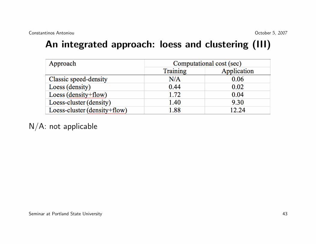
An integrated approach: loess and clustering (III)

N/A: not applicable



Thank you

Questions?

Contact information:

Constantinos Antoniou ([email protected])


On-line Calibration for Dynamic Traffic Assignment

Documents

Transcript of On-line Calibration for Dynamic Traffic Assignment