On Fixed-Point Filter Realizations - BFH · 2019-05-03 · BioMedSigProcAna On Fixed-Point Filter...
107
BioMedSigProcAna On Fixed-Point Filter Realizations Josef Goette Bern University of Applied Sciences, Biel/Bienne Institute of Human Centered Engineering - microLab [email protected] February 7, 2018 Contents 1 Introduction 1 2 Number Representations 11 3 Coefficient Quantization 34 4 Arithmetic Errors 52 4.1 Signal Quantization ................ 53 4.2 Scaling for Dynamic Range ............ 66 4.3 Pairing/Ordering in Sos Cascades ........ 87 4.4 Limit Cycles .................... 91 Symbols and Notation 97 References 104 4 Fixed-Point Filters i 2018
Transcript of On Fixed-Point Filter Realizations - BFH · 2019-05-03 · BioMedSigProcAna On Fixed-Point Filter...

BioMedSigProcAna
On Fixed-Point Filter Realizations
Josef GoetteBern University of Applied Sciences, Biel/Bienne
Institute of Human Centered Engineering - [email protected]
February 7, 2018
Contents
1 Introduction 1
2 Number Representations 11
3 Coefficient Quantization 34
4 Arithmetic Errors 524.1 Signal Quantization . . . . . . . . . . . . . . . . 534.2 Scaling for Dynamic Range . . . . . . . . . . . . 664.3 Pairing/Ordering in Sos Cascades . . . . . . . . 874.4 Limit Cycles . . . . . . . . . . . . . . . . . . . . 91
Symbols and Notation 97
References 104
4 Fixed-Point Filters i 2018

BioMedSigProcAna
c©Josef Goette, 2007–2018
All rights reserved. This work may not be translated or copied in
whole or in part without the written permission by the author, except
for brief excerpts in connection with reviews or scholarly analysis.
Use in connection with any form of information storage and retrieval,
electronic adaptation, computer software is forbidden.
4 Fixed-Point Filters ii 2018

BioMedSigProcAna
1 Introduction
Problem Statement
• floating-point filters: their design solves often only part ofdesign problem
• many real-world Dsp systems require:
– use of minimum power
– generate minimum heat
– do not induce computational overload
– ; these demands often mean: use fixed-point filters
• quantizing:
– convert floating-point filter realization into a fixed-point realization
– ; can loose filter performance and accuracy
• to do
– respect basic rules of thumb (; the art of . . . )
– simulate and determine the effects of quantization
The acronym Dsp means digital signal processing; some-times, we likewise use the same acronym to mean digital signalprocessor.
4 Fixed-Point Filters 1 2018

BioMedSigProcAna
Our present goal is to find realizations of fixed-point filtersin dedicated hardware, which fulfill requirements such as “low-power” and “small chip size.”
Concerning Matlab and its toolboxes, we note that we canwell attain our object—to design filters—with the Signal Pro-cessing Toolbox, if the object is to design floating-point filters;if we need to design fixed-point filters, however, the Dsp Sys-tem Toolbox,1 accompanied by the Fixed-Point Toolbox, is veryuseful. If we have additionally available the Filter Design HdlCoder Toolbox, we may even produce Vhdl or Verilog code forthe filters we design. Additionally there exist, to support de-sign work on the level of Simulink, the Simulink Fixed Pointtoolbox and the Simulink Hdl Coder toolbox.
1If you use an older Matlab version, we note that as of release R2011a,the previous Filter Design Toolbox and the Signal Processing Blockset havebeen merged and renamed to Dsp System Toolbox.
4 Fixed-Point Filters 2 2018

BioMedSigProcAna
Recall from ’Steps in Digital Filter Design’
1. design specifications
• frequency domain: magnitude-, phase response
• time domain: impulse-, step response, . . .
2. approximation of desired characteristics ; H(z) •—• h[n]
3. here we treat: the realization problem
4. the course on electronics treats: the implementation prob-lem
note: the above four steps are not independent; design iterations might be needed
We have already discussed the above items and their inter-relations in [Goe18, Section 6]; there we had:
The approximation problem is to find a causal, linear, time-invariant system described by its transfer function or byits impulse response.
The realization problem addresses the selection of a struc-ture that fulfills the design specifications even under finite-wordlength effects of filter coefficients and signals.
The implementation problem is the construction of the fil-ter in discrete hardware, in Vhdl coding (for integrated-circuit implementations), or in software (to run on a floa-ting-point or on a fixed-point digital signal processor).The goal of the present signal-processing and electronicscourses is to obtain Vhdl-coded implementations of fixed-point filters.
4 Fixed-Point Filters 3 2018

BioMedSigProcAna
Illustration of Problem Areas
• consider the following first-order Iir discrete-time filter
• structure
z−1
y[n− 1]a1
+x[n] y[n]
• difference equation
y[n] = a1y[n− 1] + x[n]
• transfer function
H(z) =1
1− a1z−1=
z
z − a1
4 Fixed-Point Filters 4 2018

BioMedSigProcAna
Illustration of Problem Areas (cont’d)
if the filter is implemented on a digital machine
• filter coefficient can have only a certain discrete value a1
• a1 is, in general, only an approximation of the originaldesign parameter a1 (which is a real number)
• true and desired transfer function
H(z) =z
z − a1≈ H(z) =
z
z − a1
• therefore: the true frequency response is different from thedesired frequency response
• ; coefficient-quantization problem
We note in passing that the coefficient-quantization problemis similar to the sensitivity problem encountered in the designof analog filters; there, the true values of the components donot exactly match the designed values; here, the true coefficientvalues do not exactly match the designed coefficient values.
4 Fixed-Point Filters 5 2018

BioMedSigProcAna
Illustration of Problem Areas (cont’d)
coefficient-quantization problem
• only during design process
• perturbation of h[n] •—• H(z),H(ω)
– deterministic perturbation
– system is still linear
• check the quantized design; if Nok
– do a redesign
– do a re-structuring
– allocate more bits to coefficients
– . . .
• important: the structure of a filter network has a dramaticeffect on its sensitivity to coefficient quantization
We use the acronym Nok to mean not Ok; Ok means . . . ,Ok you know it.
4 Fixed-Point Filters 6 2018

BioMedSigProcAna
Illustration of Problem Areas (cont’d)
input sampling error (analog-to-digital (Ad) conversion error)
• given analog (continuous-time) signal x(t)
• continuous-to-discrete conversion
x[n] = x(t)|t=nTs= x(t = nTs)
• amplitude discretization in Ad converter
x[n] ≈ x[n] : model: x[n] = x[n] + e[n]
• where the sequence e[n] is the Ad conversion error gener-ated by the input (amplitude-) quantization process
We denote by Ts the sampling-time interval of the assumedregular2 sampling process; correspondingly, fs = 1/Ts is thesampling frequency.
We note in passing that beside the presently considered dig-ital implementations there exist also so-called sampled-data im-plementations, which are implemented in technologies such asswitched-capacitor circuits, switched-current circuits, and thelike. In these sampled-data systems, the signals are likewisediscrete-time signals x[n]; however, these implementations havenot discrete amplitude values, but, instead, continuous ampli-tude values (continuous voltage and charge values in switched-capacitor circuits, and continuous current values in switched-current circuits). Nevertheless, also these continuous amplitude
2The samples are spaced by equal time intervals.
4 Fixed-Point Filters 7 2018

BioMedSigProcAna
values can never be exact because there is always noise in suchanalog circuits. Hence, the role played by the above quantizationnoise e[n] in digital systems is played by sampled continuous-time noise in sampled-data systems.
4 Fixed-Point Filters 8 2018

BioMedSigProcAna
Illustration of Problem Areas (cont’d)
arithmetic operations lead to quantization errors
• in our first-order Iir example
z−1
y[n− 1]v[n] a1
+x[n] y[n]
• we have v[n] = a1y[n− 1]
• result v[n] is quantized to fit the register holding the result(truncation or rounding)
• we can keep only v[n]
v[n] ≈ v[n] : model: v[n] = v[n] + ea1[n]
• where the sequence ea1[n] is the error sequence generated
by the product quantization process ; roundoff error
• properties of roundoff errors are similar to Ad-conversionerrors
• there might also be overflow errors in accumulators
It is clear that any arithmetic operation might cause overflowerrors; especially in standard filter realizations, we might have,beside overflow in accumulators, also overflow in multipliers usedto realize the filter coefficients. We have, in the above slide, not
4 Fixed-Point Filters 9 2018

BioMedSigProcAna
mentioned that kind of overflow, because usually in filter designsthe complete filter is scaled such that coefficients result whichhave absolute values that are smaller than unity. Therefore, inthe slide of page 9 for example, the signal v[n] = a1y[n − 1] issmaller than the signal y[n−1] and will not overflow if y[n−1] hasnot overflowed. Clearly, precision might be lost if not sufficientlymany bits are assigned to the result of the multiplication, butthere is, in the discussed situation, no overflow.
We note that there might be an additional error source indigital filters which are used to emulate analog filters: If the out-put signal y[n] has to be converted back to an analog signal by adigital-to-analog (Da) converter that works with fewer bits thany[n] has, we have an additional re-quantization error. Becauseof accumulation of round-off errors, we must usually allocatedmore bits to the internal arithmetic of a filter than we use atthe input x[n], and because often the output Da conversion usesthe same number of bits as the input Ad conversion does, suchre-quantization errors are not unusual.
4 Fixed-Point Filters 10 2018

BioMedSigProcAna
2 Number Representations
Overview
• generally: fixed-point ←→ floating-point
• fixed-point:
– arithmetic quantization in multipliers
– possibility of overflow in adders
• floating-point:
– arithmetic quantization in both, multipliers and adders
– practically no overflow (in stable filters)
• our goal: fixed-point filter realizations
; fixed-point number representations
Recall that our goal is to realize fixed-point filters that fulfillrequirements such as “low power” and “small chip-size.”
4 Fixed-Point Filters 11 2018

BioMedSigProcAna
Fixed-Point Number Formats
• signed magnitude
• one’s complement
• two’s complement
• offset binary
• other more special formats such as signed digit
• we only discuss the two’s-complement number format
In the present document, we only discuss the two’s-comp-lement number format—who’s binary addition is modulo addi-tion, see pages 22 ff. below—, because it is the most-commonlyused format; also, the Fixed-Point Toolbox of Matlab presentlyonly has fixed-point utilities for the two’s-complement numberformat.
Concerning the signed digit format (and other unconven-tional fixed-point number formats), you might want to consult[Kor93, Sections 2.3 and 2.4 starting on pages 21 and 24, respec-tively],3 [Mit06, Section 11.8.5 on page 639], or [MB07, Section2.2.2 on pages 57 ff.].
3If you happen to hold the newer edition of Koren’s book in your hands,you find the referenced topics in [Kor02, Sections 2.3 and 2.4 starting onpages 23 and 27, respectively].
4 Fixed-Point Filters 12 2018

BioMedSigProcAna
Examples of Fixed-Point Number Formats
decimal sign- one’s- two’s- offsetequivalent magnitude complement complement binary
7/8 0.111 0.111 0.111 1.1116/8 0.110 0.110 0.110 1.1105/8 0.101 0.101 0.101 1.1014/8 0.100 0.100 0.100 1.1003/8 0.011 0.011 0.011 1.0112/8 0.010 0.010 0.010 1.0101/8 0.001 0.001 0.001 1.0010/8 0.000 0.000 0.000 1.000
−0/8 1.000 1.111 N/A N/A−1/8 1.001 1.110 1.111 0.111−2/8 1.010 1.101 1.110 0.110−3/8 1.011 1.100 1.101 0.101−4/8 1.100 1.011 1.100 0.100−5/8 1.101 1.010 1.011 0.011−6/8 1.110 1.001 1.010 0.010−7/8 1.111 1.000 1.001 0.001−8/8 N/A N/A 1.000 0.000
these are [4, 3] bit numbers
The entries N/A in the above table mean “not available.”The notation “[4, 3] bit numbers” means that the numbers arerepresented by four bits, three of them being fractional bits, andthe forth bit, the left-most bit b3, being the sign bit, as indicatedby the following sketch:
b3 b2 b1 b0•6
binary point
4 Fixed-Point Filters 13 2018

BioMedSigProcAna
A sign bit b3 that is zero indicates a positive number, and asign bit b3 that is one indicates a negative number. Below, onpages 27 and the following, we explain in detail the notationused by Matlab and its Fixed-Point Toolbox.
We note that in the table on page 13 the formats “sign-magnitude,” “one’s complement,” and “two’s complement” allhave the same positive number representation; they only differin their representation of negative numbers:
sign-magnitude: If the sign bit is zero, b3 = 0, the 3-bit frac-tion is a positive number with magnitude
b2 · 2−1 + b1 · 2−2 + b0 · 2−3 = b2 ·1
2+ b1 ·
1
4+ b0 ·
1
8.
If the sign bit is one, b3 = 1, the 3-bit fraction is a negativenumber with the same magnitude as for the correspondingpositive number:
−(b2 · 2−1 + b1 · 2−2 + b0 · 2−3
)= −
(b2 ·
1
2+ b1 ·
1
4+ b0 ·
1
8
).
one’s complement A positive fraction is represented as in thesign-magnitude form, but a negative fraction is representedby complementing each bit of the binary representationof the corresponding positive fraction. As an example,take from the table on page 13 the number 3/8 = 0.011in sign-magnitude as well as in one’s complement and intwo’s complement; the negative in one’s complement thenis −3/8 = 1.100.
two’s complement Again, a positive fraction is representedas in the sign-magnitude form; it’s negative is obtainedby first complementing each bit of the binary represen-tation, and subsequently adding a 1 to the Lsb (least-significant bit). As an example, again take 3/8 = 0.011
4 Fixed-Point Filters 14 2018

BioMedSigProcAna
in sign-magnitude as well as in one’s complement and intwo’s complement. The complement becomes, first, 1.100(which is the one’s complement), and, second by adding anLsb, 1.101, which indeed is −3/8 in the two’s complementcolumn of the table on page 13.
offset binary The offset-binary representation is most oftenused in bipolar Da- and Ad-conversion. Referring to thetable on page 13, the offset-binary representation considersa b = 3 bit fraction with an additional sign bit as a b+1 =4 bit number representing the 2b+1 = 24 = 16 integernumbers from 0 to 15. Half of these numbers representthe negative fractions, and the other half represent thenon-negative fractions (zero and positive fractions). Notethat the two’s complement representation is converted tothe offset-binary representation, and vice versa, by simplycomplementing the sign bit b3.
4 Fixed-Point Filters 15 2018

BioMedSigProcAna
Quantization: Rounding Versus Truncation
• [3, 2] two’s-complement number example: rounding
x ∈ ℜ
xq ∈ [3, 2]-numbers
−9
8−
7
8−
5
8−
3
8
−1
8
1
8
3
8
5
8
7
8
−1
−3
4
−1
2
−1
4
1
4
1
2
3
4
000
001
010
011
111
110
101
100
The symbol ℜ stands for the set of real numbers. The [3, 2]two’s-complement numbers are numbers from the set
set =
{−1,−3
4,−1
2,−1
4, 0,
1
4,
1
2,
3
4
};
the notation “xq ∈ [3, 2]-numbers” in the above illustrationmeans that xq is a member of that set.
The dfilt objects of the Dsp System Toolbox of Matlabcan represent fixed-point filter structures;4 in this case, there is
4You just set the property Arithmetic of the filter object to ’fixed’.Of course, you must additionally have available the Fixed-Point Toolbox.
4 Fixed-Point Filters 16 2018

BioMedSigProcAna
a property RoundMode specifying how results of arithmetic op-erations are re-quantized. The above quantization with round-ing is obtained by setting RoundMode either to ’round’ or to’convergent’. These two rounding modes just distinguish them-selves in how they treat exact midpoint values; whereas ’round’rounds an exact midpoint to the closest representable numberin the direction of positive infinity, ’convergent’ rounds exactmidpoint values up only if the least significant bit (after round-ing) is set to 0. To give examples, consider the case where thebits just represent integers (or, likewise, interpret the consideredbit-string as an integer). The tie-breaking rule of ’convergent’rounding then means rounding to even integers: 17.5 is roundedto 18, as 18.5 is; -13.5 becomes -14, as does -14.5. The advan-tage of this rule is that it treats positive and negative valuesin a symmetric kind, hence does not introduce a sign bias. Al-though it is deterministic, it has some “random-like” behavior.Other notions for “convergent rounding” are “round-to-nearest-even,” “unbiased rounding,” “statistician’s rounding,” “Gaus-sian rounding,” “bankers’ rounding,” and many more.
4 Fixed-Point Filters 17 2018
BioMedSigProcAna
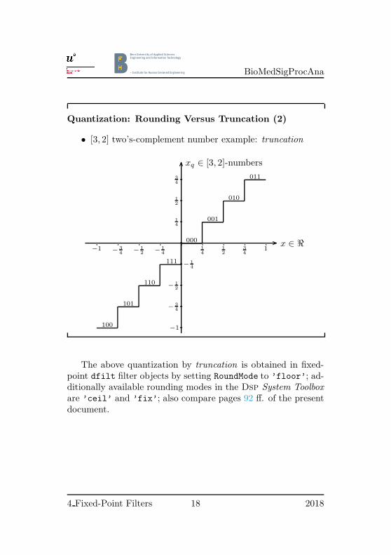
Quantization: Rounding Versus Truncation (2)
• [3, 2] two’s-complement number example: truncation
x ∈ ℜ
xq ∈ [3, 2]-numbers
−1 −3
4−
1
2−
1
4
1
4
1
2
3
41
−1
−3
4
−1
2
−1
4
1
4
1
2
3
4
000
001
010
011
111
110
101
100
The above quantization by truncation is obtained in fixed-point dfilt filter objects by setting RoundMode to ’floor’; ad-ditionally available rounding modes in the Dsp System Toolboxare ’ceil’ and ’fix’; also compare pages 92 ff. of the presentdocument.
4 Fixed-Point Filters 18 2018

BioMedSigProcAna
Quantization: Overflow Versus Saturation
• [3, 2] two’s-complement number example: saturation
x ∈ ℜ
xq ∈ [3, 2]-numbers
−9
8−
7
8−
5
8−
3
8
−1
8
1
8
3
8
5
8
7
8
−1
−3
4
−1
2
−1
4
1
4
1
2
3
4
000
001
010
011
111
110
101
100
Note: The above figure shows saturating overflow togetherwith rounding; obviously, a corresponding characteristic existsfor saturating overflow with truncation.
Fixed-point dfilt filter objects have the OverFlowMode prop-erty; set this property to ’saturate’ to obtain an arithmeticbehavior corresponding to the shown saturation characteristics.
4 Fixed-Point Filters 19 2018

BioMedSigProcAna
Quantization: Overflow Versus Saturation (2)
saturation (also often called clipping)
• normally in Ad converters
• sometimes in two’s-complement arithmetic
• size of error does not increase abruptly when overflow oc-curs
• but disadvantage: does not exploit an interesting and use-ful property of two’s-complement arithmetic (see below)
We discuss the mentioned “useful property of two’s-complementarithmetic” below on pages 22 ff..
4 Fixed-Point Filters 20 2018
BioMedSigProcAna
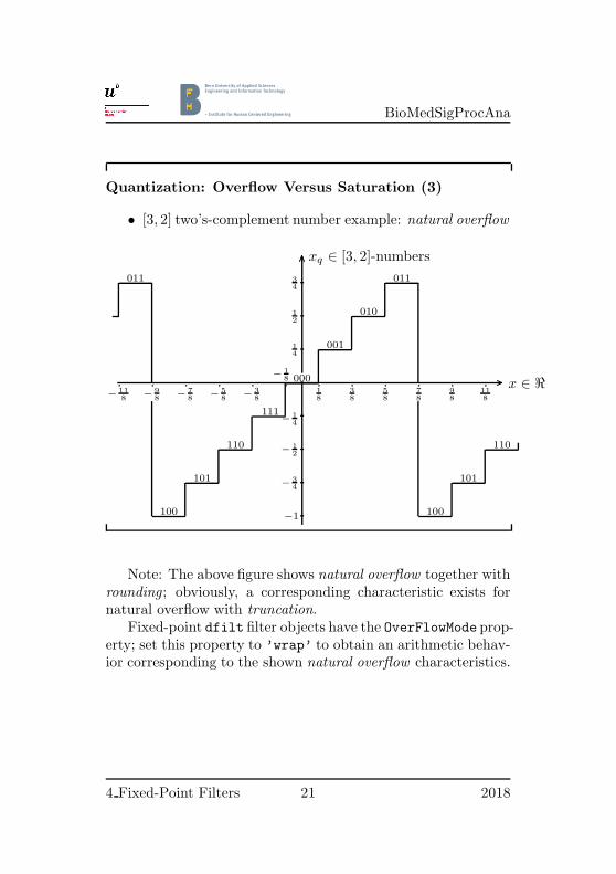
Quantization: Overflow Versus Saturation (3)
• [3, 2] two’s-complement number example: natural overflow
x ∈ ℜ
xq ∈ [3, 2]-numbers
−11
8−
9
8−
7
8−
5
8−
3
8
−1
8
1
8
3
8
5
8
7
8
9
8
11
8
−1
−3
4
−1
2
−1
4
1
4
1
2
3
4
000
001
010
011
111
110
101
100
011
100
101
110
Note: The above figure shows natural overflow together withrounding; obviously, a corresponding characteristic exists fornatural overflow with truncation.
Fixed-point dfilt filter objects have the OverFlowMode prop-erty; set this property to ’wrap’ to obtain an arithmetic behav-ior corresponding to the shown natural overflow characteristics.
4 Fixed-Point Filters 21 2018

BioMedSigProcAna
Quantization: Overflow Versus Saturation (4)
important property of two’s-complement arithmetic; only if used with natural overflow
• given: xi are two’s complement numbers in [B, L]
• given: x =∑
i xi is a two’s complement number that doesnot overflow
• then: using natural overflow, the result of accumulation iscorrect even if partial sums overflow
• because: modulo arithmetic
We just supply two simple examples to illustrate the generaltruth.
Example 1: Consider three [B, L] = [4, 3] numbers x1, x2, x3:
x1 =5
8= 0.101 ,
x2 =3
4= 0.110 ,
x3 = −1
2= 1.100 .
Then the sum of these three numbers is x1 + x2 + x3 = 7/8 andclearly is a number that does not overflow in the [4, 3] format.Depending on how we add, however, the partial sums might
4 Fixed-Point Filters 22 2018
BioMedSigProcAna
overflow; for example, we have x1 + x2 = 11/8 6∈ [4, 3]:
x1 = 0101
x2 = 01101
x1 + x2 = 1011 = −5/8← overflow .
Continuing to add to the overflowed result (x1 + x2) = −5/8the term x3, we end up with the correct overall result if we justdiscard the bit flowing over the sign bit:
x1 + x2 = 1011 = −5/8← overflowedx3 = 1100 = −1/2
1
x1 + x2 + x3 = 0111 = 7/8← correct .
Example 2: Consider all B = 3-bits combinations and inter-pret them in straightforward manner as integers:
x0 : 000 = 0x1 : 001 = 1x2 : 010 = 2x3 : 011 = 3x4 : 100 = 4x5 : 101 = 5x6 : 110 = 6x7 : 111 = 7
We thus have a set of 2B = 23 = 8 elements being the integersfrom zero to seven:
set = {x0, x1, x2, x3, x4, x5, x6, x7} = {0, 1, 2, 3, 4, 5, 6, 7} .
Now consider counting through the set by starting with zero andalways adding one; do the addition of one by straightforwardly
4 Fixed-Point Filters 23 2018

BioMedSigProcAna
adding 3-bit numbers and discarding an overflow bit if thereresults such an overflow bit:
x0 + x1 = 0 + 1 = 1 : 000
001
001
x1 + x1 = 1 + 1 = 2 : 001
001
010
x2 + x1 = 2 + 1 = 3 : 010
001
011...
x6 + x1 = 6 + 1 = 7 : 110
001
111
x7 + x1 = 7 + 1 = 8 : 111
0011 1 1
000 = 0 = 8 mod 8 .
We thus see that the straightforward binary addition with dis-regarding overflow is—for the considered B = 3-bits case—justmodulo 2B = 23 = 8 addition. We may represent the consideredset of 8 elements together with modulo 8 addition on a circle:
.....
.....
.....
.....
.....
.....
.......................................................................
.................
............................
..................................................................................................................................................................................................................................................................................................................................................................................................................
...........................................................................................................................
•000
0•001
1
• 0102
•011
3
•100
4•
101
5
•110 6
•111
7
4 Fixed-Point Filters 24 2018

BioMedSigProcAna
As far we have interpreted our eight 3-bits strings just aspositive integers. But we see that x0 = 000 is the identityelement for the addition: x0 added to any of the other elementsjust gives back this other element. Therefore, we may ask forinverses: xi + ? = 0 mod 8. We then find
1 + ? = 0 : 1 + 7 = 8 mod 8 = 0 ⇒ 7 = inverse(1) = −1 ,2 + ? = 0 : 2 + 6 = 8 mod 8 = 0 ⇒ 6 = inverse(2) = −2 ,3 + ? = 0 : 3 + 5 = 8 mod 8 = 0 ⇒ 5 = inverse(3) = −3 ,4 + ? = 0 : 4 + 4 = 8 mod 8 = 0 ⇒ 4 = inverse(4) = −4 .
The following circle-representation graphically illustrates thesefindings:
.....
.....
.....
.....
.....
.....
.......................................................................
.................
............................
..................................................................................................................................................................................................................................................................................................................................................................................................................
...........................................................................................................................
•000
0•001
1
• 0102
•011
3
•100
−4•
101
−3
•110 −2
•111
−1
Similarly, we may not only interpret our 3-bits strings as inte-gers, but likewise as fractional numbers; for the format [B, L] =[3, 2], for example, we obtain the following circle:
.....
.....
.....
.....
.....
.....
.......................................................................
.................
............................
..................................................................................................................................................................................................................................................................................................................................................................................................................
...........................................................................................................................
•000
0•001
1
4
• 0101
2
•011
3
4
•100
−1•
101
− 3
4
•110 − 1
2
•111
− 1
4
4 Fixed-Point Filters 25 2018

BioMedSigProcAna
Note that we have not shown in the above graphic the bi-nary point after the leftmost bit—the sign bit in the considered[B, L] = [3, 2] format—, because this binary point is just aninterpretation aid, but does not really exist in the arithmetic.
Finally, we return to our point of departure. If we compute,for example, in the two’s-complement system [B, L] = [3, 0] withthe elements
set = {x0, x1, x2, x3, x4, x5, x6, x7} = {−4,−3,−2,−1, 0, 1, 2, 3} ,
we correctly obtain any sum x =∑
i xi with x in the given set,independently of whether partial sums are outside the set—haveoverflow—or not, if we use the natural overflow rule. This isbecause using natural overflow we indeed do the correspondingmodulo arithmetic.
We finally note that the discussed property of two’s-com-plement arithmetic with natural overflow greatly simplifies thescaling of fixed-point (digital) filters; compare Subsection 4.2,especially see the definition of “critical nodes” on page 67.
4 Fixed-Point Filters 26 2018
BioMedSigProcAna
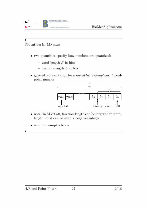
Notation in Matlab
• two quantities specify how numbers are quantized:
– word-length B in bits
– fraction-length L in bits
• general representation for a signed two’s-complement fixed-point number
bB−1 bB−2 b3 b2 b1 b0•6
binary point6
sign bit6
Lsb
L︷ ︸︸ ︷
B︷ ︸︸ ︷
• note: in Matlab, fraction-length can be larger than word-length, or it can be even a negative integer
• see our examples below
4 Fixed-Point Filters 27 2018

BioMedSigProcAna
Notation in Matlab (cont’d)
• decimal value represented by bits in [B, L] format
value = −bB−1 · 2B−L−1 + bB−2 · 2B−L−2 + · · ·
· · ·+ b1 · 2−L+1 + b0 · 2−L
bB−1 bB−2 b3 b2 b1 b0•6
binary point6
sign bit6
Lsb
L︷ ︸︸ ︷B−L−1︷ ︸︸ ︷
B︷ ︸︸ ︷
• note: L is the negative of the weight of the Lsb: 2−L
; step size = precision, does not depend on word length
• B − L− 1 defines the interval of representable numbers
numbers ∈[−2B−L−1, 2B−L−1
)
We denote left-closed, right-open sets by [xmin, xmax); thusx ∈ [xmin, xmax) means xmin ≤ x < xmax.
4 Fixed-Point Filters 28 2018

BioMedSigProcAna
Notation in Matlab (cont’d)
• example: [B, L] = [3, 2] ; B − L− 1 = 0
011 = −0 · 20 + 1 · 2−1 + 1 · 2−2 = 3/4
010 = −0 · 20 + 1 · 2−1 + 0 · 2−2 = 1/2
001 = −0 · 20 + 0 · 2−1 + 1 · 2−2 = 1/4
000 = −0 · 20 + 0 · 2−1 + 0 · 2−2 = 0
111 = −1 · 20 + 1 · 2−1 + 1 · 2−2 = −1/4
110 = −1 · 20 + 1 · 2−1 + 0 · 2−2 = −1/2
101 = −1 · 20 + 0 · 2−1 + 1 · 2−2 = −3/4
100 = −1 · 20 + 0 · 2−1 + 0 · 2−2 = −1
• represented numbers ∈ [−1, 1)
number set =
{−1,−3
4,−1
2,−1
4, 0,
1
4,
1
2,
3
4
}
Note that the interval of representable numbers is given byB − L− 1:
[−2B−L−1, 2B−L−1
)=[−20, 20
)= [−1, 1).
The precision (resolution) is 2−L = 2−2 = 1/4.
4 Fixed-Point Filters 29 2018

BioMedSigProcAna
Notation in Matlab (cont’d)
• example: [B, L] = [3, 1] ; B − L− 1 = 1
011 = −0 · 21 + 1 · 20 + 1 · 2−1 = 3/2
010 = −0 · 21 + 1 · 20 + 0 · 2−1 = 2/2
001 = −0 · 21 + 0 · 20 + 1 · 2−1 = 1/2
000 = −0 · 21 + 0 · 20 + 0 · 2−1 = 0
111 = −1 · 21 + 1 · 20 + 1 · 2−1 = −1/2
110 = −1 · 21 + 1 · 20 + 0 · 2−1 = −2/2
101 = −1 · 21 + 0 · 20 + 1 · 2−1 = −3/2
100 = −1 · 21 + 0 · 20 + 0 · 2−1 = −4/2
• represented numbers ∈ [−2, 2)
number set =
{−4
2,−3
2,−2
2,−1
2, 0,
1
2,
2
2,
3
2
}
Note that the interval of representable numbers is given byB − L− 1:
[−2B−L−1, 2B−L−1
)=[−21, 21
)= [−2, 2).
The precision (resolution) is 2−L = 2−1 = 1/2.
4 Fixed-Point Filters 30 2018

BioMedSigProcAna
Notation in Matlab (cont’d)
• example: [B, L] = [3, 3] ; B − L− 1 = −1
011 = −0 · 2−1 + 1 · 2−2 + 1 · 2−3 = 3/8
010 = −0 · 2−1 + 1 · 2−2 + 0 · 2−3 = 2/8
001 = −0 · 2−1 + 0 · 2−2 + 1 · 2−3 = 1/8
000 = −0 · 2−1 + 0 · 2−2 + 0 · 2−3 = 0
111 = −1 · 2−1 + 1 · 2−2 + 1 · 2−3 = −1/8
110 = −1 · 2−1 + 1 · 2−2 + 0 · 2−3 = −2/8
101 = −1 · 2−1 + 0 · 2−2 + 1 · 2−3 = −3/8
100 = −1 · 2−1 + 0 · 2−2 + 0 · 2−3 = −4/8
• represented numbers ∈[−1
2,
1
2
)
number set =
{−4
8,−3
8,−2
8,−1
8, 0,
1
8,
2
8,
3
8
}
Note that the interval of representable numbers is given byB − L− 1:
[−2B−L−1, 2B−L−1
)=[−2−1, 2−1
)= [−1/2, 1/2).
The precision (resolution) is 2−L = 2−3 = 1/8.
4 Fixed-Point Filters 31 2018

BioMedSigProcAna
Notation in Matlab (cont’d)
• example: [B, L] = [3, 4] ; B − L− 1 = −2
011 = −0 · 2−2 + 1 · 2−3 + 1 · 2−4 = 3/16
010 = −0 · 2−2 + 1 · 2−3 + 0 · 2−4 = 2/16
001 = −0 · 2−2 + 0 · 2−3 + 1 · 2−4 = 1/16
000 = −0 · 2−2 + 0 · 2−3 + 0 · 2−4 = 0
111 = −1 · 2−2 + 1 · 2−3 + 1 · 2−4 = −1/16
110 = −1 · 2−2 + 1 · 2−3 + 0 · 2−4 = −2/16
101 = −1 · 2−2 + 0 · 2−3 + 1 · 2−4 = −3/16
100 = −1 · 2−2 + 0 · 2−3 + 0 · 2−4 = −4/16
• represented numbers ∈[−1
4,
1
4
)
number set =
{− 4
16,− 3
16,− 2
16,− 1
16, 0,
1
16,
2
16,
3
16
}
Note that the interval of representable numbers is given byB − L− 1:
[−2B−L−1, 2B−L−1
)=[−2−2, 2−2
)= [−1/4, 1/4).
The precision (resolution) is 2−L = 2−4 = 1/16.
4 Fixed-Point Filters 32 2018

BioMedSigProcAna
Notation in Matlab (cont’d)
• example: [B, L] = [3,−2] ; B − L− 1 = 4
011 = −0 · 24 + 1 · 23 + 1 · 22 = 12
010 = −0 · 24 + 1 · 23 + 0 · 22 = 8
001 = −0 · 24 + 0 · 23 + 1 · 22 = 4
000 = −0 · 24 + 0 · 23 + 0 · 22 = 0
111 = −1 · 24 + 1 · 23 + 1 · 22 = −4
110 = −1 · 24 + 1 · 23 + 0 · 22 = −8
101 = −1 · 24 + 0 · 23 + 1 · 22 = −12
100 = −1 · 24 + 0 · 23 + 0 · 22 = −16
• represented numbers ∈ [−16, 16)
number set = {−16,−12,−8,−4, 0, 4, 8, 12}
Note that the interval of representable numbers is given byB − L− 1:
[−2B−L−1, 2B−L−1
)=[−24, 2−4
)= [−16, 16).
The precision (resolution) is 2−L = 2−(−2) = 4.
4 Fixed-Point Filters 33 2018

BioMedSigProcAna
3 Coefficient Quantization
Coefficient Quantization: Realizable Poles
• first insight into problem of coefficient quantization
• gained by studying quantization effect on pole (and zero)locations in z-plane
• more general: formal definitions of coefficient sensitivitymeasures
• here: available real-pole locations for first-order filters
• here: available complex-pole locations for second-order,
direct form filters (note: depends on structure!)
We note that the structure of the filter implementation isimportant for the present discussion; therefore, the qualifica-tion “direct form” above is important. Also note that we laterdiscuss an alternative structure, likewise only for second-orderfilters, the normal form structure on pages 47 ff.; we restrict itsdiscussion to second order, because second-order building blocksare most often used to implement higher-order filters in parallelform, see page 44, or in cascade form, see page 45.
4 Fixed-Point Filters 34 2018

BioMedSigProcAna
Realizable 1st-Order Real Poles
• direct-form filter structure
• transfer function H(z) =1
1 + az−1=
z
z + a
• coefficient a quantized as a [4, 3] two’s-complement number
• only “stable” poles (absolute values < 1) are shown
.....
.....
.....
.....
.....
.....
.....
...................................................................................................
.................
......................
.................................................
....................................................................................................................................................................................................................................................................................................................................................................................................................................................................................................................
............................................................................................................................................................................× ×××××××××××××××
z-plane
4 Fixed-Point Filters 35 2018

BioMedSigProcAna
Realizable 2nd-Order Complex Poles
• direct-form filter structure
• transfer function H(z) =1
1 + a1z−1 + a2z−2
• a1, a2 quantized as [5, 3] two’s-complement numbers
• only “stable” complex poles (absolute values ≤ 1) areshown
.....
.....
.....
.....
.....
.....
.....
...................................................................................................
.................
......................
.................................................
....................................................................................................................................................................................................................................................................................................................................................................................................................................................................................................................
............................................................................................................................................................................
×
×
×
×
×
×
×
×
×
×
×
×
×
×
×
×
×
×
×
×
×
×
×
×
×
×
×
×
×
×
×
×
×
×
×
×
×
×
×
×
×
×
×
×
×
×
×
×
×
×
×
×
×
×
×
×
×
×
×
×
×
×
×
×
×
×
×
×
×
×
×
×
×
×
×
×
×
×
×
×
×
×
×
×
×
×
×
×
×
×
×
×
×
×
×
×
×
×
×
×
×
×
×
×
×
×
×
×
×
×
×
×
×
×
×
×
×
×
×
×
×
×
×
×
×
×
×
×
×
×
×
×
×
×
×
×
×
×
×
×
×
×
×
×
×
×
×
×
×
×
×
×
×
×
×
×
×
×
×
×
×
×
×
×
×
×
×
×
×
×
×
×
×
×
×
×
×
×
×
×
×
×
×
×
×
×
×
×
×
×
×
×
×
×
×
×
×
×
×
×
×
×
×
×
×
×
×
×
×
×
×
×
×
×
×
×
×
×
×
×
×
×
×
×
×
×
×
×
×
×
×
×
×
×
×
×
×
×
×
×
×
×
×
×
×
×
×
×
×
×
×
×
×
×
×
×
×
×
×
×
×
×
×
×
×
×
×
×
×
×
×
×
×
×
×
×
×
×
×
×
×
×
×
×
×
×
×
×
×
×
×
×
×
×
×
×
×
×
×
×
×
×
×
×
×
×
×
×
×
×
×
×
×
×
×
×
×
×
×
×
×
×
×
×
×
×
×
×
×
×
×
×
×
×
×
×
×
×
×
×
×
×
×
×
×
×
×
×
×
×
×
×
z-plane
If a second-order system has real poles, it can be decomposedinto two first-order systems (with real coefficients); therefore, forreal poles the discussion of first-order systems applies, and wehave omitted the real poles in the above diagram.
We note that in the vicinity of z = 1 and in the vicinity ofz = −1 the realizable poles are not very dense. This observationshas some important consequences on the design of low- and high-pass filters, see our discussion starting on page 39.
4 Fixed-Point Filters 36 2018

BioMedSigProcAna
Realizable 2nd-Order Complex Poles (cont’d)
• why?
• transfer function
H(z) =1
1 + a1z−1 + a2z−2=
1
(1− pz−1) (1− p∗z−1)
• coefficients ←→ poles:
(1− pz−1
) (1− p∗z−1
)= 1− (p + p∗) z−1 + pp∗z−2
therefore: a1 = − (p + p∗) = −2ℜ{p}
a2 = pp∗ = |p|2
See the next page for the conclusions from the above relationsbetween coefficients and poles.
4 Fixed-Point Filters 37 2018

BioMedSigProcAna
Realizable 2nd-Order Complex Poles (cont’d)
• we have from a1 = −2ℜ{p}: quantization of a1 quantizesthe real part of the poles
• we have from a2 = |p|2: quantization of a2 quantizes theradius of the poles ; non-uniform spacing
...........
.................................................................................
.............................
......................................
......................................................................................................................................................................................................................................................................................................................................................................................................................................................................................................................................................................................
.........................................
............................................................................................................................................................................................................................................................................................................................................................................................................................................................. ............................................................................................................................................................................................................................................................................................................................................................................................................................................................... .................................................................................................................................................................................................................................................................................................................................................................................................................................................................................................................................................................... ......................................................................................................................................................................................................................................................................................................................................................................................................................................................................................................................................................................................................................................................... ................................................................................................................................................................................................................................................................................................................................................................................................................................................................................................................................................................................................................................................................................................................................... ....................................................................................................................................................................................................................................................................................................................................................................................................................................................................................................................................................................................................................................................................................................................................................................................................... .....................................................................................................................................................................................................................................................................................................................................................................................................................................................................................................................................................................................................................................................................................................................................................................................................................................................................
z-plane
example:
a1 and a2 eachquantized to [5,3]two’s complementnumbers
4 Fixed-Point Filters 38 2018
BioMedSigProcAna
Realizable 2nd-Order Complex Poles (cont’d)
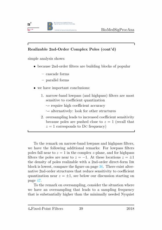
simple analysis shows:
• because 2nd-order filters are building blocks of popular
– cascade forms
– parallel forms
• we have important conclusions:
1. narrow-band lowpass (and highpass) filters are mostsensitive to coefficient quantization
; require high coefficient accuracy
; alternatively: look for other structures
2. oversampling leads to increased coefficient sensitivitybecause poles are pushed close to z = 1 (recall thatz = 1 corresponds to Dc frequency)
To the remark on narrow-band lowpass and highpass filters,we have the following additional remarks: For lowpass filterspoles fall near to z = 1 in the complex z-plane, and for highpassfilters the poles are near to z = −1. At these locations z = ±1the density of poles realizable with a 2nd-order direct-form Iirblock is lowest, compare the figure on page 36. There exist alter-native 2nd-order structures that reduce sensitivity to coefficientquantization near z = ±1, see below our discussion starting onpage 47.
To the remark on oversampling, consider the situation wherewe have an oversampling that leads to a sampling frequencythat is substantially higher than the minimally needed Nyquist
4 Fixed-Point Filters 39 2018
BioMedSigProcAna
rate: Such a high oversampling rate pushes the spectrum of theuseful signal to the vicinity of ω = 0 (vicinity of Dc), whichcorresponds in the z-plane to the vicinity of z = 1. Obviously,the filters applied to such an oversampled signal then have toperform their work also in the vicinity of ω = 0, and, in turn,have poles pushed to the vicinity of z = 1. Because poles inthe vicinity of z = 1 lead to increased sensitivity to coefficientquantization, too much oversampling should be avoided. Thisadvice to reduce oversampling seems to be counter-intuitive at afirst glance, because reducing the sampling interval—increasingthe sampling frequency—enables the better approximation ofthe underlying continuous-time signal, and, in turn, to betterapproximate a corresponding continuous-time filter. However,although we can indeed reduce aliasing by oversampling, wepay with an increased sensitivity of the filter coefficients; ad-ditionally, the required speed of the hardware is, of course, alsoincreased—lesser time to process more data. Generally, coeffi-cient sensitivity and hardware speed are more important aspectsthan aliasing.
The approach to avoid the outlined dilemma is as follows:First, the analog-to-digital conversion is performed with someoversampling—the larger the oversampling rate, the simpler theanti-alias filtering becomes; note that the anti-aliasing filtermust precede the analog-to-digital conversion, and note thatit is an analog filter. Next, a discrete-time low-pass filteringpaves the way for a subsequent decimation—a down-samplingin discrete time; such a low-pass filtering will not influence spec-tral components of the useful signal, because we have done ananalog-to-digital conversion with large oversampling. Finally,the planed discrete-time filtering is performed on a signal withlow sampling rate, thus relaxing the demands on the the z-planepole locations.
4 Fixed-Point Filters 40 2018

BioMedSigProcAna
Coefficient Quantization: Higher Order Filters
• higher-order filters in direct form: ; analysis becomesmore complicated
• we have seen: coefficient sensitivity increases by goingfrom 1st- to 2nd-order
• guess: even more increased sensitivity for higher-order fil-ters
• well-known result from numerical analysis:
– sensitivity of roots of a polynomial to accuracy ofcoefficients increases with order of polynomial
– stability of direct-form filter might be lost due to co-efficient quantization
– even if filter remains stable: specifications might be-come violated
– for fixed-point implementations: generally avoid direct-form Iir structures
– prefer cascade or parallel forms
4 Fixed-Point Filters 41 2018

BioMedSigProcAna
Coefficient Quantization: Zeros in Fir Filters
• consider Fir filter in direct form (recall: magnitude re-sponse produced entirely by zeros)
• seem to have same sensitivity problems as Iir filters indirect form
• however: important differences to Iir situation:
– most Fir designs are for linear phase
– coefficients satisfy symmetry conditions: bk = ±bM−k
– quantizing both, bk and bM−k to same perturbedvalue
; filter is still a linear-phase filter
; only magnitude response is perturbed
– zeros on unit circle remain on unit circle
– symmetry constraint: greatly reduces sensitivity ofmost Fir filters ; direct form is widely used
• of course: parallel form does not exist
• cascade form: not widely used
We have stated above that zeros designed onto the unit cir-cle remain on the unit circle if the symmetric coefficients arequantized the same. Of course the zeros resulting from quan-tized coefficients will move along the unit circle as compared tothe ideal (designed) locations. If the quantization is so strongthat two moving zeros come together, then they will split intoreciprocal pairs and, of course, no longer stay on the unit circle.
4 Fixed-Point Filters 42 2018

BioMedSigProcAna
Concerning the parallel form of Fir filters, it is of course nottrue that it does not exist, but it just does not make much sense.Consider, as an example, the Fir transfer function H(z) = b0 +b1z
−1 + b2z−2. We might consider a parallel realization with
parallel sub-transfer functions b0, and b1z−1, and b2z
−2, butthis realization is trivial and even not efficient, because we needmore memory cells than minimum. In contrast to the Fir filtercase, we have in the Iir filter case true parallel-form realizationsvia the partial fraction decomposition of the complete rationaltransfer function; see below.
Concerning cascade forms and zeros that do not lie on theunit circle, we just state that a minimum order of 4 for thecascade blocks is needed to satisfy symmetry conditions neededfor linear-phase filters, see [Jac96, p. 377].
4 Fixed-Point Filters 43 2018

BioMedSigProcAna
Parallel Form Iir Filters
• expansion of H(z) into partial fractions
• stopband attenuation: depends mostly on having zeros onunit circle
• in parallel form: zeros are not realized by individual 1st-and 2nd-order terms
• but zeros are realized by the way how all parallel-sectiontransfer functions add together
• all coefficients (in numerator and in denominator) of allparallel-form sections affect every zero
• ; highly sensitive situation
; zeros are in no way constraint to lie on the unit circleafter quantization
• therefore: parallel form is usually avoided for filters withdemanding specifications
4 Fixed-Point Filters 44 2018

BioMedSigProcAna
Cascade Form Iir Filters
• cascade form is more robust under coefficient quantizationthan parallel form
• poles have same low sensitivity as in parallel form, butzeros are also roots of only 1st- and 2nd-order polynomials
• additionally: in common cases with zeros on the unit cir-cle, the numerator coefficients b2k are all ±1:
Bk(z) = 1 + b1kz−1 + b2kz−2 = 1 + b1kz−1 ± 1 · z−2
; b2k not changed by quantization
• although zeros on unit circle move by quantization of b1k,they do not move off the unit circle
; stopband attenuation specifications are more easily sat-isfied than in parallel form
We have assumed that the sections in the cascade form areenumerated by k, k = 1, 2, . . . , last.
Note that by stating that the zeros do not move off the unitcircle, we of course assume that the zeros on the unit circle donot become real by quantization.
To understand that a complex-conjugate zero pair on theunit circle has the coefficient b2k in the corresponding factorpolynomial Bk(z) equal to 1, we assume that we have such a
4 Fixed-Point Filters 45 2018

BioMedSigProcAna
zero pair at angles ±ω0 on the unit circle; then Bk(z) becomes
Bk(z) =(1− ejbω0z−1
)(1− e−jbω0z−1
)
= 1−(ejbω0 + e−jbω0
)z−1 + ejbω0e−jbω0
︸ ︷︷ ︸= 1
z−2 ,
indeed showing that b2k = 1. We note in passing that we alsosee that b1k becomes −2 cos(ω0).
4 Fixed-Point Filters 46 2018

BioMedSigProcAna
Normal-Form Iir Filters
• how to reduce sensitivity of poles in the vicinity of z = ±1?
• is a problem only for very narrow-band lowpass/highpassfilters
• problem with direct-form Iir biquads: realizable pole lo-cations are intersections of (evenly spaced) vertical lineswith non-evenly spaced concentric circles
; low pole-density near z = ±1
• consider the coupled form:
– from 2nd-order state-space description with input x[n]and output y[n]
s[n + 1] = As[n] + bx[n] s[n] = state vector
y[n] = cTs[n] + δx[n]
– with state-feedback matrix
A =
(α1 α2
−α2 α1
)
Don’t panic, see the next pages! For realizable pole locationsobtainable with direct-form Iir biquads, you may want to seeagain the example on pages 36 and 38.
We use bold-face lower-case letters to denote vectors andupper-case bold-face letters for matrices. The system vectors
4 Fixed-Point Filters 47 2018
BioMedSigProcAna
and/or matrices—A, b, and cT —have elements with Greek let-
ters corresponding to the Latin letter of the vector or the matrix;the vector b, as an example, has, therefore, elements βi. Alsonote that all vectors are column vectors, and that row vectorscome as transposed column vectors, like c
T .
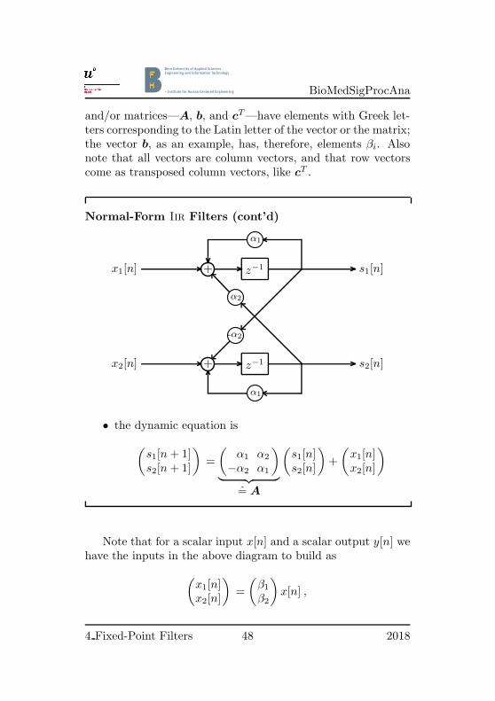
Normal-Form Iir Filters (cont’d)
+ z−1
α1
+ z−1
α1
x1[n]
x2[n]
s1[n]
s2[n]
α2
-α2
• the dynamic equation is
(s1[n + 1]s2[n + 1]
)=
(α1 α2
−α2 α1
)
︸ ︷︷ ︸= A
(s1[n]s2[n]
)+
(x1[n]x2[n]
)
Note that for a scalar input x[n] and a scalar output y[n] wehave the inputs in the above diagram to build as
(x1[n]x2[n]
)=
(β1
β2
)x[n] ,
4 Fixed-Point Filters 48 2018
BioMedSigProcAna
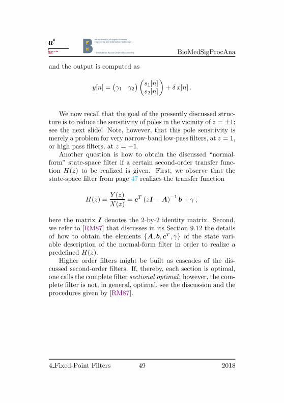
and the output is computed as
y[n] =(γ1 γ2
)(s1[n]s2[n]
)+ δ x[n] .
We now recall that the goal of the presently discussed struc-ture is to reduce the sensitivity of poles in the vicinity of z = ±1;see the next slide! Note, however, that this pole sensitivity ismerely a problem for very narrow-band low-pass filters, at z = 1,or high-pass filters, at z = −1.
Another question is how to obtain the discussed “normal-form” state-space filter if a certain second-order transfer func-tion H(z) to be realized is given. First, we observe that thestate-space filter from page 47 realizes the transfer function
H(z) =Y (z)
X(z)= c
T (zI −A)−1
b + γ ;
here the matrix I denotes the 2-by-2 identity matrix. Second,we refer to [RM87] that discusses in its Section 9.12 the detailsof how to obtain the elements {A, b, cT , γ} of the state vari-able description of the normal-form filter in order to realize apredefined H(z).
Higher order filters might be built as cascades of the dis-cussed second-order filters. If, thereby, each section is optimal,one calls the complete filter sectional optimal ; however, the com-plete filter is not, in general, optimal, see the discussion and theprocedures given by [RM87].
4 Fixed-Point Filters 49 2018

BioMedSigProcAna
Normal-Form Iir Filters (cont’d)
• for the poles and their quantization we have
poles = eigenvalues of A
= det (zI −A) = 0 : (z − α1)2
+ α22 = 0
; zp1,p2 = α1 ± jα2 ; both, α1 and α2, are quantized
...........
.................................................................................
.............................
......................................
......................................................................................................................................................................................................................................................................................................................................................................................................................................................................................................................................................................................
.........................................
................................................................................................................................
z-plane
example:
α1 and α2 eachquantized to [4,3]two’s complementnumbers
The transfer function formula in the previous page containsthe matrix inverse of (zI −A). If we evaluate it using Cramer’srule, we obtain
(zI −A)−1
=Adj (zI −A)
det (zI −A)=
Adj (zI −A)
D(z),
and we find that the denominator polynomial D(z), which givesthe poles of the filter, is likewise the polynomial that determinesthe eigenvalues of the state-feedback matrix A, hence the polesof the system equal the eignvalues of the state-feedback matrix.
4 Fixed-Point Filters 50 2018
BioMedSigProcAna
Concerning poles and zeros under coefficient quantization,the following general statements hold:
• If we have poles and/or zeros that are highly clustered,small errors in the coefficients—in the present context in-troduced by quantization5—may cause large shifts in thepoles and/or the zeros locations. Thereby, the larger thenumber of polynomial roots (poles of denominator poly-nomials, zeros of numerator polynomials) is, the greaterthe sensitivity becomes.
• In cascade-form structures and in parallel-form structureseach pair of complex-conjugate poles is realized separately;additionally in cascade-form structures, each pair of com-plex-conjugate zeros is likewise realized separately. There-fore, the error in a given pole (and zero in a cascade-formstructure) is independent of the distance from the otherpoles (and zeros). Hence, in general, cascade (or possiblyparallel) forms are to be preferred over direct forms froma point of view of coefficient quantization. This state-ment is particularly true for very selective filters that havehighly clustered poles. Because cascade-form structureshave the advantage not only for poles, but for zeros too,we generally prefer cascade-form structures over parallel-form structures.
5We recall that to realize discrete-time filters there are alternative tech-niques to digital filters: switched-capacitor or switched-current circuits andthe like; in these implementations we have errors in coefficients due tonot exactly realizable elements like capacitors, specifically ratios of capaci-tances.
4 Fixed-Point Filters 51 2018

BioMedSigProcAna
4 Arithmetic Errors
Overview
• quantization errors
– in Ad conversion
– in multipliers due to truncation or rounding
– ; quantization noise
• overflow errors: in certain internal nodes such as
– inputs to multipliers
– outputs of accumulators
– ; may lead to large amplitude oscillations
– ; probability of overflow minimized by scaling ofsignal levels
• probability of overflow↔ signal-to-noise ratio (Snr)
– more stringent signal scaling
+ probability of overflowց− Snr ց
– less stringent signal scaling
− probability of overflowր+ Snr ր
– find a compromise
4 Fixed-Point Filters 52 2018

BioMedSigProcAna
4.1 Signal Quantization
Quantization in Ad-Converters
• processing blocks and signals
-x(t)Sampler -x[n]
Quantizer -xq[n]Coder -xeq[n]
assumptions:
• x(t) and x[n] ∈ [Xmin, Xmax)
; full-scale range Xmax −Xmin = RFS
• quantizer with rounding
• coder: [B, L] = [B, B − 1] two’s-complement numbers
; xeq[n] ∈ [−1, 1), resolution δ =1
2B−1
• quantizer: resolution ∆ =RFS
2B
Note that the difference between the resolutions δ and ∆ isjust that δ gives the “abstract” resolution relative to the interval[−1, 1), whereas ∆ gives the “natural” resolution with respectto the full-scale range; if, for example, x(t) is a voltage signal,RFS comes in volts and, in turn, ∆ comes in volts too.
4 Fixed-Point Filters 53 2018
BioMedSigProcAna
Quantization in Ad-Converters (cont’d)
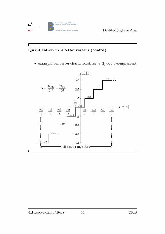
• example-converter characteristics: [3, 2] two’s complement
x[n]
xq [n]
full-scale range RFS
−
9∆
2−
7∆
2−
5∆
2−
3∆
2
−
∆
2
∆
2
3∆
2
5∆
2
7∆
2
−4∆
−3∆
−2∆
−∆
∆
2∆
3∆
000
001
010
011
111
110
101
100
∆ =RFS
2B=
RFS
23
4 Fixed-Point Filters 54 2018

BioMedSigProcAna
Quantization in Ad-Converters (cont’d)
• quantization error: signal flow graph
x[n]+
xq[n] = x[n] + e[n]
e[n]
• quantization error: characteristics for 3-bits example
x[n]
e[n]
full-scale range RFS
−
9∆
2−
7∆
2−
5∆
2−
3∆
2−
∆
2
∆
2
3∆
2
5∆
2
7∆
2
R
∆
2
M
−
∆
2
Note that the signals xq[n], x[n], and e[n] are deterministi-cally interconnected—if two of them are given, then the thirdfollows! This truth is in contrast to the probabilistic models forthe quantization noise e[n] that we introduce below. Becausethe engineering results that these ill-founded models deliver areuseful, it is common practice to nevertheless work with the mod-els.
4 Fixed-Point Filters 55 2018
BioMedSigProcAna
Quantization in Ad-Converters (cont’d)
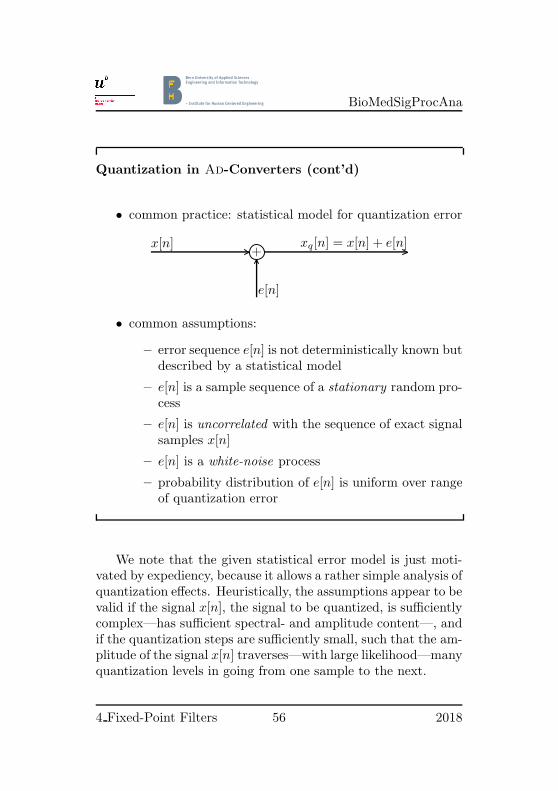
• common practice: statistical model for quantization error
x[n]+
xq[n] = x[n] + e[n]
e[n]
• common assumptions:
– error sequence e[n] is not deterministically known butdescribed by a statistical model
– e[n] is a sample sequence of a stationary random pro-cess
– e[n] is uncorrelated with the sequence of exact signalsamples x[n]
– e[n] is a white-noise process
– probability distribution of e[n] is uniform over rangeof quantization error
We note that the given statistical error model is just moti-vated by expediency, because it allows a rather simple analysis ofquantization effects. Heuristically, the assumptions appear to bevalid if the signal x[n], the signal to be quantized, is sufficientlycomplex—has sufficient spectral- and amplitude content—, andif the quantization steps are sufficiently small, such that the am-plitude of the signal x[n] traverses—with large likelihood—manyquantization levels in going from one sample to the next.
4 Fixed-Point Filters 56 2018

BioMedSigProcAna
Quantization in Ad-Converters (cont’d)
• quantization error model:
; some commonly used probability distributions
e
pd(e)
1/∆
−
∆
2
∆
20
rounding
me = 0
σ2e = ∆2/12
e
pd(e)
1/∆
−∆ 0
two’s complementtruncation
me = −∆/2
σ2e = ∆2/12
e
pd(e)
1/(2∆)
−∆ ∆0
one’s complementtruncation
me = 0
σ2e = ∆2/3
• mean values of error samples me
• variances of error samples σ2e
In the above plots, the acronym “pd” stands for probabilitydistribution.
Note that rounding yields the given symmetric probabilitydistribution function for two’s complement as well as for one’scomplement.
4 Fixed-Point Filters 57 2018

BioMedSigProcAna
Arithmetic Quantization: Roundoff Noise
• basic arithmetic operations involved in (linear) digital fil-ter implementations are
; multiplication and addition
• in fixed-point implementations:
; multiplication results must be rounded or truncated
; addition results need not to be rounded or truncated
(but addition results might overflow ; scaling for dynamicrange)
• truncation and rounding:
; product quantizations
; nonlinear processes
• common practice:
; use statistical quantization-noise models as in Ad con-version
We here consider only linear filters; therefore, the involvedoperations are only multiplication and addition. Note, however,that many adaptive filters—which are not linear filters—alsojust need these two basic operations; other adaptive filters useadditional computations. For the discussion of finite-precisioneffects in adaptive filters we refer to [Hay96].
The mentioned statistical quantization-noise model of Adconverters is the one discussed on pages 56 and 57.
4 Fixed-Point Filters 58 2018
BioMedSigProcAna
Roundoff Noise Analysis
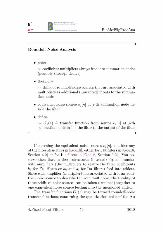
• note:
; coefficient multipliers always feed into summation nodes(possibly through delays)
• therefore:
; think of roundoff-noise sources that are associated withmultipliers as additional (unwanted) inputs to the summa-tion nodes
• equivalent noise source ej[n] at j-th summation node in-side the filter
• define:
; Gj(z) = transfer function from source ej[n] at j-thsummation node inside the filter to the output of the filter
Concerning the equivalent noise sources ej [n], consider anyof the filter structures in [Goe18], either for Fir filters in [Goe18,Section 4.2] or for Iir filters in [Goe18, Section 5.2]. You ob-serve then that in these structures (internal) signal brancheswith amplifiers (the multipliers to realize the filter coefficientsbk for Fir filters or bk and al for Iir filters) feed into adders.Since each amplifier (multiplier) has associated with it an addi-tive noise source to describe the round-off noise, the totality ofthese additive noise sources can be taken (summed) together toone equivalent noise source feeding into the mentioned adder.
The transfer functions Gj(z) may be termed roundoff-noisetransfer functions; concerning the quantization noise of the Ad
4 Fixed-Point Filters 59 2018

BioMedSigProcAna
converter, the complete filter transfer function H(z) acts as thenoise transfer function for its quantization noise.
Roundoff Noise Analysis (cont’d)
• equivalent roundoff-noise system
Gj(z)ej [n]
GN (z)eN [n]
G1(z)e1[n]
e2[n]
•
•
•
+output
4 Fixed-Point Filters 60 2018

BioMedSigProcAna
Roundoff Noise Analysis (cont’d)
• output-noise spectrum due to roundoff noise
Sout(ω) =∑
j
∣∣Gj(ejω)∣∣2 σ2
j
where σ2j = variance of equivalent roundoff
white-noise source ej [n]
• output-noise power due to roundoff noise
σ2out =
1
2π
∫ π
−π
Sout(ω) dω
= output-noise variance
The Dsp System Toolbox of Matlab supplies the commandnoisepsd() to compute the noise power spectral density at a fil-ter’s output caused by roundoff noise inside the filter. The aver-age power of the output noise (the integral of the power spectraldensity) can be computed with the command avgpower().
4 Fixed-Point Filters 61 2018

BioMedSigProcAna
Roundoff Noise Analysis (cont’d)
• variance σ2j of equivalent noise source ej[n]:
• if we have
σ20 = variance of a single multiplier
rounding operation
• : rounding before summation
kj = number of multipliers inputtingto j-th summation node
• then the variance of the equivalent noise source ej [n] is
σ2j = kjσ
20
• if rounding is performed after summation: kj = 1
4 Fixed-Point Filters 62 2018

BioMedSigProcAna
Signal-to-Noise Ratios (Snr)
• noise sources
– Ad-conversion noise at the filter input
– roundoff noise inside the filter
• signal-to-noise ratios (Snr)
Snr = 10 log10
(σ2
sig
σ2noise
)
where σ2sig = signal variance representing
average power of signal
σ2noise = noise variance representing
average power of noise
• general goals:
– as small as possible noise
– as large as possible Snr
4 Fixed-Point Filters 63 2018

BioMedSigProcAna
Signal-to-Noise Ratios (cont’d)
• at filter input
Snr = 10 log10
(σ2
x
σ2AD
)
where x[n] = input signal with variance σ2x
σ2AD = variance of Ad-conversion noise
• at filter output
Snr = 10 log10
(σ2
y
σ2noise
)
where y[n] = output signal of filter due to input signalx[n], variance σ2
y
σ2noise = σ2
out + σ2AD,out
σ2out = noise variance due to roundoff noise
σ2AD,out = variance of Ad-conversion noise transferred
to output
The variance σ2out is the variance of the complete roundoff
noise as it appears at the filter output; for its computation com-pare page 61. Correspondingly, σ2
AD,out describes the varianceof the Ad-conversion quantization noise as it appears at the out-put of the filter. Because the Ad-conversion noise at the filterinput is modeled as a white noise with variance σ2
AD, the filter
4 Fixed-Point Filters 64 2018

BioMedSigProcAna
with its transfer function H(z) transforms this white input noiseto a colored output noise with spectral density
SAD,out(ω) =∣∣H(ejω)
∣∣2 σ2AD .
The corresponding variance of the Ad-conversion noise trans-ferred to the filter output—its average power—thus becomes
σ2AD,out =
1
2π
∫ π
−π
SAD,out(ω) dω
=σ2
AD
2π
∫ π
−π
∣∣H(ejω)∣∣2 dω .
Furthermore note that the theory assumes the Ad-conversionnoise source and the various roundoff-noise sources to be uncor-related; therefore, the total noise variance at the filter output,σ2
noise, is just the sum of the noise variances of the total round-off noise and the Ad-conversion noise, both transferred to theoutput of the filter.
4 Fixed-Point Filters 65 2018

BioMedSigProcAna
4.2 Scaling for Dynamic Range
Why We Need Scaling
• to increase Snr
; increase signal levels at all nodes inside the filter
• because:
roundoff-noise level is fixed for a given structure and agiven resolution
• but: increasing signal levels too much leads to
– exceeding of dynamic range of fixed-point arithmetic
– ; overflows result in certain computations
– overflow is a severe nonlinearity
– ; preclude overflow
Or
; make its probability acceptably small and mini-mize the resulting distortions
To minimize the effect of—low probable—overflow, use sat-uration at plus/minus full scale instead of wrapping, also seepage 96.
4 Fixed-Point Filters 66 2018

BioMedSigProcAna
Critical Nodes
• it seems that we must ensure that signals do not overflowat any node inside the filter
• fortunately, not true (in two’s complement) because:
– some nodes separated only by delays
– summation of more than two numbers:
if total sum is small enough not to overflow
then the correct sum results regardless of order inwhich numbers are added
; independent of overflows that may occur in thepartial sums or even if some of the inputs to adderhave themselves overflowed as a result of multiplica-tion with a coefficient larger than one
Concerning nodes that are separated only by one or moredelays—which are memory cells in a realization—it is clear thatif a signal does not overflow at the input, it will not overflow atthe output.
The statement that the result of a summation, that lies in thedynamic range of the arithmetic, may have overflows in partialsums without doing harm, is true in any modulo arithmetic suchas two’s-complement arithmetic; see, for example, [Jac96] andthe references given therein.
4 Fixed-Point Filters 67 2018

BioMedSigProcAna
Fir Filters in Direct Form
• simplest to start with; structure
z−1
x[n−M ]bM +
z−1
x[n− k]bk +
z−1
x[n− 1]b1 +
b0x[n]
y[n]
• (finite) impulse response h[k]: {b0, b1, . . . , bM}
4 Fixed-Point Filters 68 2018

BioMedSigProcAna
Fir Filters in Direct Form (cont’d)
• assumption: available dynamic range (full scale) is R
input |x[n]| ≤ R , all n
• output
y[n] =∑
k
h[k]x[n− k] = convolution sum
• then
|y[n]| =∣∣∣∣∣∑
k
h[k]x[n− k]
∣∣∣∣∣
≤∑
k
|h[k]| |x[n− k]|
≤ R∑
k
|h[k]|
Concerning the available dynamic range—the full scale—theparameter R is often taken as 1, that is, one often assumes thatthe input signal values are in the interval [−1, 1).
Note that in the presently considered case of an Fir filter,the convolution summation is over finitely many terms. In themore general case of a filter containing feedback terms, the con-volution sum will include infinitely many terms. Also note thatthe present formulation neglects the additional roundoff-errorinputs ej [n]; they are small in any case.
4 Fixed-Point Filters 69 2018

BioMedSigProcAna
Fir Filters in Direct Form (cont’d)
• then:
output y[n] is also in available dynamic range |y[n]| ≤ R
• ifl1 =
∑
k
|h[k]| ≤ 1
• l1 is called the l1-norm of the Fir filter
• if l1 6≤ 1 then scale:
• scale factor s =1
l1
• scale the coefficients h[k] , k = 1, 2, . . . , M
h[k] = s · h[k] =1
l1· h[k]
• then: new Fir filter h[k] has no overflows
Note that scaling the coefficients of the original filter h[k]with the scale factor s is equivalent to amplifying the inputsignal x[n] with a gain s. For s < 1 this amplification is, ofcourse, an attenuation.
4 Fixed-Point Filters 70 2018

BioMedSigProcAna
Fir Filters in Direct Form (cont’d)
• by proposed scaling:
input signal x[n] is multiplied by s = 1/l1
• for s < 1: attenuation
• for s < 1: Snr ց
• ; of interest: scale factor s as large as possible
• to scale, there are other—less stringent—norms often used
– l2 = L2 norm
– L∞ norm
• choice of scaling norm: a compromise between
low probability of overflow←→ large Snr
Note that if we use, on one hand, the l1-norm for scaling,as is exemplified on pages 69–70, then we are sure to have nooverflow. If we use, on the other hand, some other norms forscaling, then there is a certain—low—probability for overflow.
Concerning other norms used in filter scaling, we give on thepages 72 and 73 the available norms of the Dsp System Toolboxof Matlab.
4 Fixed-Point Filters 71 2018

BioMedSigProcAna
Norms Used in the Dsp System Toolbox
• consider a filter with impulse response h[k]:
discrete-time domain h[k] •—• H(ω) frequency domain
• discrete-time domain norms
l1-norm : l1 =∑
k
|h[k]|
l2-norm : l2 =
√∑
k
(h[k]
)2
l∞-norm : l∞ = maxk|h[k]|
We note that the norms defined here apply not only to Firfilters, but, likewise, to Iir filters. Whereas for Fir filters theindex k in the above formulae runs over finitely many integers,it runs over infinitely many integers in the more general case ofIir filters.
If we need to preclude overflow with certainty, we must usel1-norm scaling which yields, however, the lowest Snr.
The l2-norm scaling is the same as the L2-norm scaling in-troduced below, see page 73.
4 Fixed-Point Filters 72 2018

BioMedSigProcAna
Norms Used in the Dsp System Toolbox (cont’d)
• frequency domain norms
L1-norm : L1 =1
2π
∫ π
−π
|H(ω)| dω
L2-norm : L2 =
√1
2π
∫ π
−π
∣∣H(ω)∣∣2dω
L∞-norm : L∞ = maxω|H(ω)|
• relation between these norms
l1 ≥ L∞ ≥ L2 = l2 ≥ L1 ≥ l∞
• identity L2 = l2 is due to Parseval’s theorem
If we use L∞-norm scaling, then we preclude overflow for apure sinusoidal signal in steady state. The L∞-norm is, how-ever, the most conservative of the frequency-domain constraints,because it assumes that, in the worst case, the input power isconcentrated at a single frequency. Overflows are very unlikelywith L∞-norm scaling.
For many broadband input signals, L∞-norm scaling is tooconservative. In these cases it might be better to use an L2-normscaling—which is the same as an l2-norm scaling—to obtain alarger Snr and still have a low probability of overflow.
4 Fixed-Point Filters 73 2018
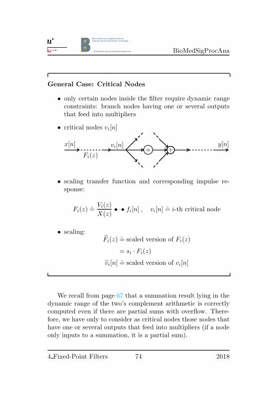
BioMedSigProcAna
General Case: Critical Nodes
• only certain nodes inside the filter require dynamic rangeconstraints: branch nodes having one or several outputsthat feed into multipliers
• critical nodes vi[n]
x[n]
Fi(z)
vi[n]α +
y[n]
• scaling transfer function and corresponding impulse re-sponse:
Fi(z) =Vi(z)
X(z)•—• fi[n] , vi[n] = i-th critical node
• scaling:Fi(z) = scaled version of Fi(z)
= si · Fi(z)
vi[n] = scaled version of vi[n]
We recall from page 67 that a summation result lying in thedynamic range of the two’s complement arithmetic is correctlycomputed even if there are partial sums with overflow. There-fore, we have only to consider as critical nodes those nodes thathave one or several outputs that feed into multipliers (if a nodeonly inputs to a summation, it is a partial sum).
4 Fixed-Point Filters 74 2018

BioMedSigProcAna
General Case: Absolute Bound Scaling
• assumption: available dynamic range (full scale) is R
input |x[n]| ≤ R ,
• then
vi[n] =∑
k
fi[k]x[n− k] = convolution sum
• then
|vi[n]| =∣∣∣∣∣∑
k
fi[k]x[n− k]
∣∣∣∣∣
≤∑
k
|fi[k]| |x[n− k]|
≤ R∑
k
|fi[k]|
Concerning the available dynamic range—the full scale—again note that the parameter R is often taken as 1, that is,one often assumes that the input signal values are in the inter-val [−1, 1).
Note that in the presently considered case of a general Iirfilter, the convolution summation is over infinitely many terms.Furthermore, the given convolution formulation assumes zeroinitial conditions and neglects small roundoff-error inputs ej [n].
4 Fixed-Point Filters 75 2018

BioMedSigProcAna
General Case: Absolute Bound Scaling (cont’d)
• if: scaled version vi[n] of vi[n] must satisfy constraint
|vi[n]| ≤ R , for all critical nodes
• then: we must scale the filter such that
l1,i =∑
k
∣∣∣fi[k]∣∣∣ ≤ 1 , for all critical nodes
• this is l1 scaling
• simplest scaling: multiply (attenuate/amplify) input sig-nal by
s =1
maxi
l1,i
where l1,i =∑
k
∣∣∣fi[k]∣∣∣ , fi[k] •—• Fi(z)
= l1-norm of i-th scaling transfer function Fi(z)
To numerically compute the l1-norm of an Fir filter is sim-ple, because the computation involves only finitely many sam-ples of its impulse response. In the general case of an Iir filter,however, the impulse response has infinitely many terms and wemight numerically approximate it as follows: Iteratively com-pute, for L = 1, 2, . . ., partial sums l1,L =
∑Lk=0 |fi[k]|, and stop
the computation if the difference l1,L− l1,(L−1) becomes smallerthan a pre-specified limit; a typical value of the limit might be10−6.
4 Fixed-Point Filters 76 2018

BioMedSigProcAna
General Case: Alternative Scaling Rules
• above scaling rule
– based on worst case
– does not fully utilize dynamic range of all adder out-puts
– ; reduces Snr significantly
• more practical scaling rules
– use another norm
l1 ≥ L∞ ≥ L2 = l2 ≥ L1 ≥ l∞
– for a selected norm to work with, say ℓ, let
ℓi = ℓ-norm of Fi(z) •—• fi[k] , unscaled
ℓi = ℓ-norm of Fi(z) •—• fi[k] , scaled
– then, after scaling, obtain
ℓi ≤ 1 , for all critical nodes
– withFi(z) = siFi(z) =⇒ si ≤
1
ℓi
The above scaling constants si denote the cumulative scal-ings that are applied to nodes vi[n].
For the norms given in the above slide we refer to pages 72and 73.
4 Fixed-Point Filters 77 2018

BioMedSigProcAna
General Case: Alternative Scaling Rules (cont’d)
more practical scaling rules (cont’d)
• exploit special structures
• most important structures: Sos cascades
; scale individual blocks
• Signal Processing Toolbox of Matlab: command scale()
; automatic scaling of Sos cascades with one of the norms
l1 ≥ L∞ ≥ L2 = l2 ≥ L1 ≥ l∞
• also see the following example
Again we refer to pages 72 and 73 for the definitions of thenorms enumerated in the slide above.
We say above that you should “see” the example on pages 79–86, and you might find the exemplified scaling to involve quitetedious computations. But note that the computations are fullydeterministic (algorithmic), and that in a practical applicationthe Dsp System Toolbox command scale() will free you fromdoing the scaling by hand.
4 Fixed-Point Filters 78 2018
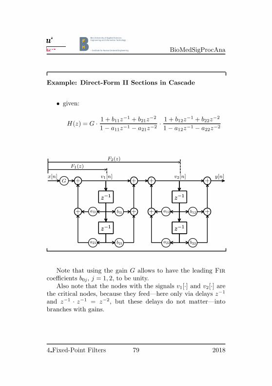
BioMedSigProcAna
Example: Direct-Form II Sections in Cascade
• given:
H(z) = G · 1 + b11z−1 + b21z
−2
1− a11z−1 − a21z−2· 1 + b12z
−1 + b22z−2
1− a12z−1 − a22z−2
x[n]G
z−1
a21
z−1
a11+
+
z−1
b21
z−1
b11 +
+
z−1
a22
z−1
a12+
+
z−1
b22
z−1
b12 +
+y[n]v1[n] v2[n]
F1(z)
F2(z)
Note that using the gain G allows to have the leading Fircoefficients b0j , j = 1, 2, to be unity.
Also note that the nodes with the signals v1[·] and v2[·] arethe critical nodes, because they feed—here only via delays z−1
and z−1 · z−1 = z−2, but these delays do not matter—intobranches with gains.
4 Fixed-Point Filters 79 2018

BioMedSigProcAna
Example (cont’d): Scaling Transfer Functions
• recall
H(z) = G · 1 + b11z−1 + b21z
−2
1− a11z−1 − a21z−2︸ ︷︷ ︸
= H1(z)
· 1 + b12z−1 + b22z
−2
1− a12z−1 − a22z−2︸ ︷︷ ︸
= H2(z)
• critical nodes: v1[n] and v2[n]
• scaling transfer functions (from input to critical nodes)
F1(z) =G
1− a11z−1 − a21z−2
F2(z) = H1(z) · G
1− a12z−1 − a22z−2
where H1(z) =1 + b11z
−1 + b21z−2
1− a11z−1 − a21z−2
4 Fixed-Point Filters 80 2018

BioMedSigProcAna
Example (cont’d): Norms
• select a norm to work with, say ; ℓ
• example: if we would use the L∞ norm, then ℓ = L∞
• then we have the following ℓ-norms of the relevant transferfunctions
ℓ-norm of F1(z) : ℓF1
ℓ-norm of F2(z) : ℓF2
ℓ-norm of H(z) : ℓH
4 Fixed-Point Filters 81 2018
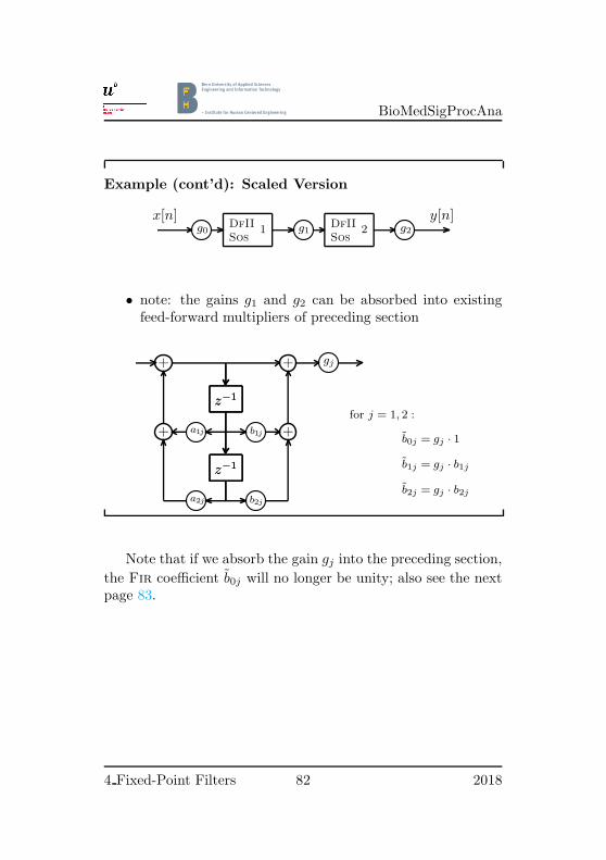
BioMedSigProcAna
Example (cont’d): Scaled Version
x[n]g0
DfIISos
1 g1DfIISos
2 g2
y[n]
• note: the gains g1 and g2 can be absorbed into existingfeed-forward multipliers of preceding section
z−1
a2j
z−1
a1j+
+
z−1
b2j
z−1
b1j +
+ gj
for j = 1, 2 :
b0j = gj · 1
b1j = gj · b1j
b2j = gj · b2j
Note that if we absorb the gain gj into the preceding section,
the Fir coefficient b0j will no longer be unity; also see the nextpage 83.
4 Fixed-Point Filters 82 2018

BioMedSigProcAna
Example (cont’d): Scaled Version (cont’d)
• in detail, we obtain for the scaled structure
x[n]G
z−1
a21
z−1
a11+
+
z−1
b21
z−1
b11 +
b01 +
z−1
a22
z−1
a12+
+
z−1
b22
z−1
b12 +
b02 +y[n]v1[n] v2[n]
F1(z)
F2(z)
Note that the above scaled structure has new values for thefeed-forward multipliers bij , i = 0, 1, 2, j = 1 for the first and
j = 2 for the second section; also note that new multipliers b0j
have been introduced.If the zeros of the transfer function are on the unit circle, as
is usually the case in practical filters, these (complex-conjugate)zeros zz = ejϕ and z∗z = e−jϕ yield numerators of the form(1− zzz
−1) (
1− z∗zz−1)
= 1−(zz + z∗z ) z−1+z−2, that is, values
for b2j that are unity. In such cases the choice b0j = b2j = 2−β,which is an approximation, might be useful to reduce the totalnumber of true multipliers (recall that multiplying by 2−β is justa shift); of course, we pay for this simplification with a slightdecrease in the Snr.
4 Fixed-Point Filters 83 2018
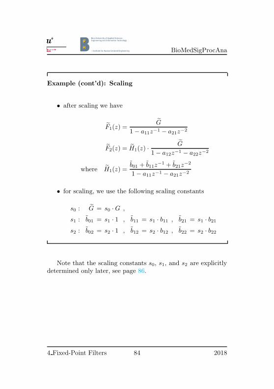
BioMedSigProcAna
Example (cont’d): Scaling
• after scaling we have
F1(z) =G
1− a11z−1 − a21z−2
F2(z) = H1(z) · G
1− a12z−1 − a22z−2
where H1(z) =b01 + b11z
−1 + b21z−2
1− a11z−1 − a21z−2
• for scaling, we use the following scaling constants
s0 : G = s0 ·G ,
s1 : b01 = s1 · 1 , b11 = s1 · b11 , b21 = s1 · b21
s2 : b02 = s2 · 1 , b12 = s2 · b12 , b22 = s2 · b22
Note that the scaling constants s0, s1, and s2 are explicitlydetermined only later, see page 86.
4 Fixed-Point Filters 84 2018

BioMedSigProcAna
Example (cont’d): Scaling (cont’d)
• relations between scaled and unscaled transfer functions
F1(z) =G
1− a11z−1 − a21z−2=
s0 ·G1− a11z−1 − a21z−2
= s0 · F1(z)
F2(z) = H1(z) · G
1− a12z−1 − a22z−2
=(s1 ·H1(z)
)( s0 ·G1− a12z−1 − a22z−2
)
=(s0 · s1
)F2(z)
H(z) = G H1(z) H2(z) =(s0G
)(s1H1(z)
)(s2H2(z)
)
=(s0s1s2
)G H1(z) H2(z)
=(s0s1s2
)H(z)
4 Fixed-Point Filters 85 2018
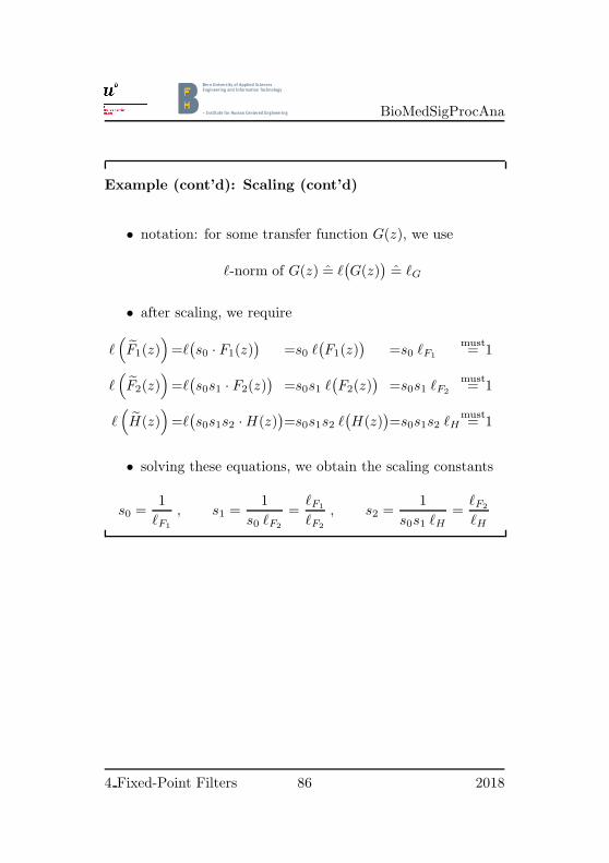
BioMedSigProcAna
Example (cont’d): Scaling (cont’d)
• notation: for some transfer function G(z), we use
ℓ-norm of G(z) = ℓ(G(z)
)= ℓG
• after scaling, we require
ℓ(F1(z)
)=ℓ(s0 · F1(z)
)=s0 ℓ
(F1(z)
)=s0 ℓF1
must= 1
ℓ(F2(z)
)=ℓ(s0s1 · F2(z)
)=s0s1 ℓ
(F2(z)
)=s0s1 ℓF2
must= 1
ℓ(H(z)
)=ℓ(s0s1s2 ·H(z)
)=s0s1s2 ℓ
(H(z)
)=s0s1s2 ℓH
must= 1
• solving these equations, we obtain the scaling constants
s0 =1
ℓF1
, s1 =1
s0 ℓF2
=ℓF1
ℓF2
, s2 =1
s0s1 ℓH=
ℓF2
ℓH
4 Fixed-Point Filters 86 2018

BioMedSigProcAna
4.3 Pairing/Ordering in Sos Cascades
An important question to answer when designing digital Iir fil-ters in form of second-order-section (Sos) cascades is, whichpoles should be paired together with which zeros, and, how thesepole-zero pairs, which each make up a second-order section, havefinally to be ordered inside of the complete Sos cascade.
Problem Formulation
• Iir filter in Sos-cascade structure
• question 1: how to order individual sections?
• question 2: how to pair poles and zeros?
• goals
– minimize probability of overflow
– maximize Snr
• only rule of thumb solutions
; depends on norm used for scaling
There are many ways to represent a filter in second-ordersection form. Through careful pairing of the poles and zeros,careful ordering of the sections in the cascade, and multiplica-tive scaling of the sections, it is possible to reduce quantizationnoise gain and avoid overflow in some fixed-point filter imple-mentations. The functions zp2sos() and ss2sos() of the Signal
4 Fixed-Point Filters 87 2018

BioMedSigProcAna
Processing Toolbox of Matlab perform pole-zero pairing, sec-tion scaling, and section ordering; we refer to the Linear SystemTransformations available in the Signal Processing Toolbox.6
6 The function zp2sos() transforms a filter specified by its zeros andpoles to a cascade of second-order sections; correspondingly, the functionss2sos() transforms a filter specified by its state-space description to a cas-cade of second-order sections. The function tf2sos(), which transforms afilter specified by its transfer function to a cascade of second-order sections,does also ordering, but it does it by calling zp2sos().
4 Fixed-Point Filters 88 2018

BioMedSigProcAna
With L∞-Norm Scaling
• select ordering of sections
• select pairing of poles and zeros
• according to following rules:
1. start with last section in (remaining) cascade
; it must obtain
• complex-conjugate pole-pair closest to the unit circle
• combine that pole-pair with the zero-pair that is clos-est to it
2. for remaining sections
• continue with rule (1)
• until all sections are defined
If we use the command7 scale() of the Dsp System Toolboxof Matlab, we may, as an option, indicate the desired ordering;if we do not indicate the ordering, scale() does an automaticordering which adapts to the given situation. The commandreorder() rearranges the order of the sections in a second-ordersection filter. See also our hints on page 87.
7Note that scale() works only for the special but practically most im-portant class of second-order-section (Sos) filters.
4 Fixed-Point Filters 89 2018

BioMedSigProcAna
With L2-Norm Scaling
• ordering rule opposite to rule for L∞-norm scaling
• pairing rule same as rule for L∞-norm scaling
• select ordering of sections
• select pairing of poles and zeros
• according to following rules:
1. start with first section in (remaining) cascade
; it must obtain
• complex-conjugate pole-pair closest to the unit circle
• combine that pole-pair with the zero-pair that is clos-est to it
2. for remaining sections
• continue with rule (1)
• until all sections are defined
See our hints on pages 87 and 89.
4 Fixed-Point Filters 90 2018

BioMedSigProcAna
4.4 Limit Cycles
What are Limit Cycles
• as far: roundoff-error analysis based on assumption of un-correlated errors ; statistical noise model
• is Ok for most signals
– signals with sufficient spectral content
– signals with sufficient amplitude content
• however
– problems for low-level inputs
– problems for periodic input signals that are synchro-nized with sampling rate
• then: roundoff errors cannot be assumed to be white noise
• then: linear roundoff-noise model cannot explain behavior
• extreme and important case: zero or constant input signal
– ideally: output of stable Dt filter would asymptoti-cally approach zero or a constant
– but: consider example below
We abbreviate discrete time by Dt.The mentioned example starts on page 92 and ends on page 94.
4 Fixed-Point Filters 91 2018

BioMedSigProcAna
What are Limit Cycles: Example8
• given: first-order recursive filter
y[n] = −0.5y[n− 1] + x[n] ,
x[n] = 0 , zero input signal
y[0] = 7/8 , initial state
• given:
– state y[n] is represented as a [B, L] = [4, 3] two’s-complement number
– coefficient −0.5 is represented as a [B, L] = [2, 1]two’s-complement number
– arithmetic with rounding (see comments in text)
It is intuitively clear, that the nonlinear behavior introducedby quantization strongly depends on how the quantization isdone. For the example-results shown on the page 94 we haveused “rounding to the nearest” with the exact midpoint roundedto the closest representable number in the direction of largermagnitude. This corresponds to the Matlab integer roundingcommand round(), which produces, for example, round(-3.5)= -4; so we have computed, for example, y[1] = round((7/8) ∗(−1/2)) = round(−7/16) = round(−3.5/8) = −4/8. We note,however, that the Fixed Point Toolbox of Matlab, on which the
8The Fixed-Point Toolbox of Matlab has a demo on limit cycles, whichis called filimitcycledemo.m. You find it in the Help window via a searchto ‘‘limit cycles’’; see in Demo Search Results.
4 Fixed-Point Filters 92 2018

BioMedSigProcAna
Dsp System Toolbox bases for fixed-point filter implementations,does it slightly different: Setting the rounding mode to ’round’
will round to the closest representable number, with the exactmidpoint rounded to the closest representable number in thedirection of positive infinity;9 if we set the rounding mode to’convergent’, it also rounds to the nearest allowable quantizedvalue, but exact midpoint values are rounded up only if the leastsignificant bit (after rounding) would be set to 0.
Other available rounding modes in the Dsp System Toolboxare ’ceil’, ’fix’, and ’floor’; ’ceil’ rounds to the closestrepresentable number in the direction of positive infinity; ’fix’rounds to the closest representable number in the direction ofzero; and ’floor’, which is equivalent to truncation, roundsto the closest representable number in the direction of negativeinfinity. For details consult the manuals.
9In our example we would then obtain y[1] = round((7/8) ∗ (−1/2)) =round(−7/16) = round(−3.5/8) = −3/8.
4 Fixed-Point Filters 93 2018

BioMedSigProcAna
What are Limit Cycles: Example (cont’d)
• then: we obtain
n 0 1 2 3 4 5 6
ideal y[n]7
8− 7
16
7
32− 7
64
7
128− 7
256
7
512
real y[n]7
8−4
8
2
8−1
8
1
8−1
8
1
8
• real y[n]
– does not converge to zero
– oscillates ; periodic output = limit cycles
• for the [4, 3] two’s-complement represented state with round-ing computations we have
quant
(2−3/2
1− |−0.5|
)= quant
(1/16
1/2
)=
1
8
; dead band =
(−1
8,1
8
)
Concerning dead-band computations, it can be shown thatfor a general first-order system
y[n] = a · y[n− 1] + x[n] ,
4 Fixed-Point Filters 94 2018

BioMedSigProcAna
the dead-band (−yd, yd) is given for [B, L] two’s-complementnumber computations with rounding as
yd = quant
(2−L/2
1− |a|
).
Note that for a > 0 the resulting limit cycles are constants (aDc signal), whereas for a < 0 the signs alternate, giving thus aoscillatory signal with (maximum) radian frequency ω = π.
For second-order systems the analysis becomes more compli-cated but is still feasible. For higher-order systems with parallelrealizations of second-order blocks, the outputs of the individ-ual second-order blocks are independent when the input is zero,thus the second-order system analysis can directly be applied.In the case of cascade realizations, however, only the first sec-tion has a zero input, and succeeding sections may exhibit othercharacteristic limit cycles or may just filter the limit cycles gen-erated in the first section. In any case, the limit cycle behaviorof higher-order systems becomes much more complex, and, cor-respondingly, the analysis becomes much more complicated. Tolearn more about limit cycles and their analysis, you might wantto consult one of [OS89], [Jac96], [RM87], or [Mit98], and theliterature cited therein.
Roberts and Mullis [RM87] discuss in Section 9.17 constant-input limit cycles and indicate measures to reduce limit-cycleeffects. Such countermeasures include the addition of a smallamount of noise (“dither”) in the computation, or to use magni-tude truncation instead of rounding. Mitra discusses limit cyclesin [Mit98, Section 9.2]. He indicates, with references to addi-tional literature, that random rounding is a technique to sup-press zero-input limit cycles. Furthermore, he introduces limit-cycle free structures and indicates that most general approachesbase on state-space structures. A recent paper [YAK08] dis-cussing limit-cycle free structures indicates that limit cycles andtheir suppression are still open research problems.
4 Fixed-Point Filters 95 2018

BioMedSigProcAna
Overflow Oscillations
• above, there are rounding limit cycles:
– can always be reduced to an acceptable level
– by increasing number of bits used to represent signal
• another form of autonomous oscillations:
– produced by overflow characteristics of two’s-comple-ment arithmetic
– oscillations consume entire dynamic range of filter
– must be avoided
– usual scaling: does minimize probability of overflow,but does not preclude it entirely
– solution: modify accumulator to implement a satu-ration arithmetic
; but not saturating in partial sum computations,only saturating the resulting total
The above statements are likewise true for one’s-complementcomputations.
We finally note that the following notions are also often used:
• small-scale limit cycles, which are due to quantization;
• large-scale limit cycles, which are due to overflow.
4 Fixed-Point Filters 96 2018

BioMedSigProcAna
Notation and Symbols
ai Feedback coefficients (in an Iir filter); depending onthe context, the feedback coefficients might also ap-pear with double indices as aij .
A(z) Denotes the denominator polynomial of a discrete-time transfer function.
A State-feedback matrix of a system in state-space de-scription; see page 47.
bi Feed-forward coefficients (Fir filter or Fir-part ofan Iir filter); depending on the context, the feed-forward coefficients might also appear with doubleindices as bij . But note that bi might also denote bitnumber i.
b Input weight vector of a system in state-space de-scription; see page 47.
B Usually denotes the number of bits in a fixed-pointnumber.
B(z) Denotes the numerator polynomial of a discrete-timetransfer function.
[B, L] Matlab notation for a fixed-point B-bits two’s com-plement number having L fraction bits; see page 27.
c Output vector of a system in state-space description;see page 47.
e[·] Usually denotes a discrete-time error signal.
ej Equivalent noise source at j-th summation node; seethe model for the round-off noise analysis, page 59.
4 Fixed-Point Filters 97 2018
BioMedSigProcAna
f Natural frequency of continuous-time signals in Hz.
f Natural frequency of discrete-time signals. Note thatf is a dimensionless quantity: f = f/fs where fs isthe sampling frequency.
fs Sampling frequency; fs = 1/Ts; see page 7.
fi[k] Impulse response corresponding to scaling transferfunction Fi(z): fi[k] •—• Fi(z); see page 74.
Fi(z) Scaling transfer function number i; see page 74.
gi Scaling gains in an Sos cascade; see page 82.
G As a scalar it denotes a gain; see page 79.
Gj(z) Transfer function from j-th summation node insideof the filter to its output; see the model for theround-off noise analysis, page 59.
h[k] Impulse response of a discrete-time linear system.The impulse response and the transfer function ofthe system are a z-transformation pair: h[k] •—•H(z).
h[k] Impulse response of scaled filter that had before scal-ing the impulse response h[k]; see page 70.
H(z) Transfer function of a discrete-time linear system.The the transfer function and the impulse responseof the system are a z-transformation pair: h[k] •—•H(z).
I Identity matrix of appropriate dimension; see page 50.
j Usually is the complex unit, j =√−1; we use j
sometimes also as an index variable, but the contextmakes clear what is the correct interpretation.
4 Fixed-Point Filters 98 2018

BioMedSigProcAna
l1 Denotes the l1 norm of a filter, which is defined inthe time domain; for an Fir filter see page 70; forthe more general case see page 72.
l2 Denotes the l2 norm of a filter, which is defined inthe time domain; see page 72.
l∞ Denotes the l∞ norm of a filter, which is defined inthe time domain; see page 72.
L Usually denotes the number of fractional bits in afixed-point number.
L1 Denotes the L1 norm of a filter, which is defined inthe frequency domain; see page 73.
L2 Denotes the L2 norm of a filter, which is defined inthe frequency domain; see page 73.
L∞ Denotes the L∞ norm of a filter, which is defined inthe frequency domain; see page 73.
me Mean of the random variable e; see page 57.
n Variable to denote discrete-time.
p Often used to denote a pole of a system.
pd(·) Probability distribution; see page 57.
quant(·) Quantized value of number.
RFS Full-scale range; see page 53. We note that some-times we abbreviate RFS to just R.
s Scaling factor; see page 70. Often, scaling factorsappear with subscripts, as in si.
s[·] State vector of a discrete-time system in state-spacedescription; see page 47.
4 Fixed-Point Filters 99 2018

BioMedSigProcAna
Sout(ω) Noise spectral density at the output of a filter; seepage 61.
t Variable to denote continuous time.
T As superscript indicates vector- and matrix trans-pose.
Ts Sample time interval; Ts = 1/fs; see page 7.
vi[·] Signal at critical node number i; see page 74. Crit-ical nodes are a concept in the realm of scaling fordynamic range.
vi[·] Signal at critical node number i after scaling; seepage 74.
x[·] Discrete-time signal; see page 7.
xq[·] Discrete-time signal which is quantized in amplitude;see page 53.
xeq[·] Discrete-time signal which is quantized in amplitude,and which is described by a certain code word in theinterval [−11); see page 53.
x(·) Continuous-time signal; see page 7.
[xmin, xmax) Left-closed, right-open set: x ∈ [xmin, xmax) thusmeans xmin ≤ x < xmax; compare page 28.
y[·] Discrete-time signal; usually an output signal of asystem.
z Complex variable of the z transformation.
αi The scalar elements of state-feedback matrix A of astate variable description of a filter; see page 47.
4 Fixed-Point Filters 100 2018

BioMedSigProcAna
βi The scalar elements of the input vector b of a statevariable description of a filter; see page 47 and thefollowing.
γi The scalar elements of the output vector cT of a state
variable description of a filter; see page 47 and thefollowing.
δ “Abstract” resolution; see page 53. Also used for ascalar feed-through term in a state variable descrip-tion of a filter; see page 47 and the following.
∆ “Natural” resolution; see page 53.
σ2e Variance of the random variable e.
σ2out Noise power at the output of a filter; see page 61.
σ2sig Average power of a signal; see page 63.
σ2noise Average noise power; see page 63.
σ2AD Average of Ad-conversion noise; see page 64.
σ2AD,out Average of Ad-conversion noise transferred to the
output of a considered system; see page 64.
σ2x Average power of signal x[·]; see page 64.
ω Radian frequency of continuous-time signals, ω =2πf where f denotes the natural frequency in Hz.
ω Radian frequency of discrete-time signals. As f , thediscrete-time radian frequency is likewise dimension-less: ω = ωTs = 2πf/fs, where ω, Ts, and fs denotethe radian frequency of continuous-time signals, thesampling interval, and the sampling frequency, re-spectively.
4 Fixed-Point Filters 101 2018

BioMedSigProcAna
ℓ A generic norm selected to be used for a specificscaling; see page 77. With subscript, ℓH is the ℓ-norm of the (partial) filter with transfer function H .
H(ω) Frequency response of a filter with transfer functionH(z): H(ω) = H(z = ejω).
ℜ{·} ℜ{z} gives the real part of the complex number z.
· We use the tilde applied to a quantity to mean thatthe quantity is scaled. As an example, take an im-pulse response h[k] of some filter before scaling; thefilter after scaling will realize the scaled impulse re-sponse h[k].
| · | Denotes the absolute value.
[·) Left-closed, right-open sets: x ∈ [xmin, xmax) meansthat xmin ≤ x < xmax; see page 28.
4 Fixed-Point Filters 102 2018

BioMedSigProcAna
We next list (some of) the used abbreviations. The list isto be understood as “work in progress;” we do not yet have allabbreviations, but we are willing to constantly improve this list.
Ad Analog-to-digital (converter); see page 7.
Ct Continuous time.
Da Digital-to-analog (converter); see page 10.
DfII Direct-form II (Iir filter).
Dsp Digital signal processing, or digital signal proces-sor; see page 1.
Dt Discrete time, see page 91.
Fir Finite impulse response (filter).
Hdl Hardware description language; denotes any com-puter or programming language for the formal de-scription of (mainly digital) electronic circuits.
Iir Infinite impulse response (filter).
Lsb Least-significant bit.
Msb Most-significant bit.
N/A Not available; see page 13.
Nok Not Ok.
Ok All correct.
pd(·) Probability distribution; see page 57.
Snr Signal-to-noise ratio, see page 52.
Sos Second-order section, see page 78.
Vhdl Very high speed integrated circuit hardware de-scription language.
4 Fixed-Point Filters 103 2018

BioMedSigProcAna
References
[Goe18] Josef Goette. Biomedical Signal Processing andAnalysis—Filtering for Removing Artifacts. Bern Uni-versity of Applied Sciences, Script at the Bfh-tiBiel/Bienne, HuCE-microLab, February 2018.
[Hay96] Simon Haykin. Adaptive Filter Theory. Prentice-HallInc., Englewood Cliffs, N.J., 3rd edition, 1996.
[Jac89] Leland B. Jackson. Digital Filters and Signal Process-ing. Kluwer Academic Publishers, Amsterdam, 2ndedition, 1989.
[Jac96] Leland B. Jackson. Digital Filters and Signal Process-ing with Matlab Exercises. Kluwer Academic Pub-lishers, Amsterdam, fifth printing 2002, 3rd edition,1996.
[Kor93] Israel Koren. Computer Arithmetic Algorithms.Prentice-Hall Inc., Englewood Cliffs, N.J., 1993.
[Kor02] Israel Koren. Computer Arithmetic Algorithms. A KPeters, Ltd., Natick, MA, 2nd edition, 2002.
[MB04] Uwe Meyer-Baese. Digital Signal Processing with FieldProgrammable Gate Arrays. Springer Verlag, BerlinHeidelberg New York, 2nd edition, 2004.
[MB07] Uwe Meyer-Baese. Digital Signal Processing with FieldProgrammable Gate Arrays. Springer Verlag, BerlinHeidelberg New York, 3rd edition, 2007.
[Mit98] Sanjit K. Mitra. Digital Signal Processing: A Com-puter Based Approach. Mc Graw Hill, New York, 1998.Bfh-ti Biel/Bienne Library 621.391 MITRA.
4 Fixed-Point Filters 104 2018
BioMedSigProcAna
[Mit06] Sanjit K. Mitra. Digital Signal Processing: A Com-puter Based Approach. Mc Graw Hill, New York, 3rdedition, 2006. Bfh-ti Biel/Bienne Library 621.391MITRA.
[OS89] Alan V. Oppenheim and Ronald W. Schafer. Discrete-Time Signal Processing. Prentice-Hall Inc., Engle-wood Cliffs, N.J., 1989. Bfh-ti Biel/Bienne Library621.391 OPPEN.
[RM87] Richard A. Roberts and Clifford T. Mullis. Digital Sig-nal Processing. Addison-Wesley Publishing Co., Read-ing, Mass., 1987.
[YAK08] Shunsuke Yamaki, Masahide Abe, and MasayukiKawamata. On the absence of limit cycles in state-space digital filters with minimum L2-sensitivity.IEEE Trans. Circuits Syst. II, 55(1):46–50, January2008.
4 Fixed-Point Filters 105 2018