ON ESTIMATING THE EXPECTED RETURN ON THE...

Journal of Financial Economics 8 (1980) 323-361. 0 North-Holland Publishing Company

ON ESTIMATING THE EXPECTED RETURN ON THE MARKET

An Exploratory Investigation*

Robert C. MERTON

Mussuchusetts Institute of Technology, Cumbridge, MA 02139, USA

Received April 1980, revised version received July 1980

The expected market return is a number frequently required for the solution of many investment and corporate tinance problems, but by comparison with other tinancial variables, there has been little research on estimating this expected return. Current practice for estimating the expected market return adds the historical average realized excess market returns to the current observed interest rate. While this model explicitly reflects the dependence of the market return on the interest rate, it fails to account for the effect of changes in the level of market risk. Three models of equilibrium expected market returns which reflect this dependence are analyzed in this paper. Estimation procedures which incorporate the prior restriction that equilibrium expected excess returns on the market must be positive are derived and applied to return data for the period 19261978. The principal conclusions from this exploratory investigation are: (1) in estimating models of the expected market return, the non-negativity restriction of the expected excess return should be explicitly included as part of the specification; (2) estimators which use realized returns should be adjusted for heteroscedasticity.

1. Introduction

Modern finance theory has provided many insights into how security prices are formed and has provided a quantitative description for the risk structure of equilibrium expected returns. In the most basic form of the Capital Asset Pricing Model,’ this equilibrium structure is given by the Security Market Line relationship; namely,

(1.1)

*Aid from the Debt and Equity project of the National Bureau of Economic Research, and the National Science Foundation is gratefully acknowledged. Any opinions expressed are not those of either the National Bureau of Economic Research or the National Science Foundation. My thanks to F. Black and J. Cox for many helpful discussions and to R. Henriksson for scientific assistance. I sincerely appreciate the editorial suggestions of E. Fama, M. Jensen, and G. W. Schwert.

‘See Sharpe (1964). Lintner (1965), and Mossin (1966). For an excellent survey article on the Capital Asset Pricing Model, see Jensen (1972).

324 R.C. Merton, Estimating the expected return on the market

where ai and a denote the expected rate of return on security i and the market portfolio, respectively; I is the riskless interest rate; and pi is the ratio of the covariance of the return on security i with the return on the market divided by the variance of the return on the market. This same basic model tells us that all efficient or optimal portfolios can be represented by a simple combination of the market portfolio with the riskless asset. Hence, if a’ and cre are the expected rate of return and standard deviation of return on an efftcient portfolio, then ae = w(a-r)+r and ~=WU where w is the fraction

allocated to the market and e is the standard deviation of the return on the market. From these conditions, we have that the equilibrium tradeoff between risk and return for efficient portfolios is given by

ae-r=[(x-r)/a]cf. (1.2)

(1.2) is called the Capital Market Line and (a-r)/o, the slope of that line, is called the Price of Risk.

From (1.1) and (1.2), one can determine the optimal portfolio allocation for an investor and the proper discount rate to employ for the evaluation of securities. Moreover, these equations provide the critical ‘cost of capital’ or ‘hurdle rates’ necessary for corporate capital budgeting decisions. Of course, (1.1) and (1.2) apply only for the most basic version of the CAPM, and indeed, empirical tests of the Security Market Line have generally found that while there is a positive relationship between beta and average excess return, there are significant deviations from the predicted relationship.’ However, these deviations appear principally in very ‘high’ and very ‘low’ beta securities. Moreover, there is some question about the validity of these tests3 The more sophisticated intertemporal and arbitrage-model versions of the CAPM4 show that the equilibrium expected returns on securities may depend upon other types of risk in addition to ‘systematic’ or ‘market’ risk, and hence, they provide a theoretical foundation for (1.1) and (1.2) not to obtain. However, in all of these models, the market risk of a security will affect its equilibrium expected return, and indeed, for most common stocks, market risk will be the dominant factor.’ Thus, at least for common stocks and broad-based equity portfolios, the basic model as described by (1.1) and (1.2) should provide a reasonable ‘first approximation’ theory for equilibrium expected returns.

%ee Jensen (1972), Black, Jensen and &holes (1972), Fama and MacBeth (1974), and Friend and Blume (1970).

‘See Roll (1977). %ee Breeden (1979), Cox, Ingersoll and Ross (forthcoming), Long (1974), Ross (1976), Merton

(1973 and forthcoming h). sBy ‘dominant factor’, we do not mean that most of the variation in an individual stock’s

realized returns can be ‘explained’ by the variation in the market’s return. Rather, we mean that among the systematic risk factors that influence an individual stock’s equilibrium expected return, the market risk of that stock will have the largest influence on its expected return.

R.C. Merton, Estimating the expected return on the market 325

Of course, all one needs to know to apply these formulas in solving portfolio and corporate financial problems are the parameter values. And as might be expected, considerable effort has been applied to estimating them. However, this effort has not been uniform with respect to the different parameters, and as will be shown, this non-uniformity is not without good reason.

For the most part, the nominal riskless interest rate, r, is an observable, and so that parameter need not be estimated. Among the other parameters, beta is the one most widely estimated. In dozens of academic research papers, betas have been estimated for individual stocks; portfolios of stocks; bonds and other fixed income securities; other investments such as real estate; and even human capital.6 For practitioners, there are beta ‘books’ and beta services. While for the most part these betas are estimated from time series of past returns, various accounting data have also been used.

In their pioneering work on the pricing of options and corporate liabilities,

Black and Scholes (1973) deduced an option pricing formula whose only non-observable input is the variance rate on the underlying stock. As a result, there has been a surge in research effort to estimate the variance rates for returns on both individual stocks and the market. Although this research activity is still in its early stages of development, variance rate estimates are already available from a number of sources.

In contrast, there has been little academic research on estimating the expected return on either individual stocks or the market. Ibbotson and Sinquefield (1976, 1979) have carefully cataloged the historical average returns on stocks and bonds from 1926 to 1978. However, they provide no model as to how expected returns change through time. There is no literature analogous to the term structure of interest rates for the expected return on stocks, although there is research going on in this direction as, for

example, in Cox, Ingersoll, and Ross (forthcoming). One possible explanation for this paucity of research on expected returns

is that for many applications within finance, only relative pricing

relationships are used, and therefore, estimates of the expected returns are not required. Some important examples of such applications are option and corporate liabilities pricing and the testing for superior performance of actively-managed portfolios. However, for many if not most applications, an estimate of the expected return on the market is essential. For example, to implement even the most passive strategy of portfolio allocation, an investor must know the expected return on the market and its standard deviation in order to choose an optimal mix between the market portfolio and the riskless asset. Indeed, even if one has superior security analysis skills so that the optimal portfolio is no longer a simple mix of the market and the riskless

‘See Fama and Schwert (1977a).


asset, Treynor and Black (1973) have shown that the optimal strategy will still involve mixing the market portfolio with an active portfolio, and the optimal mix between the two will depend upon the expected return and standard deviation of the market. For a corporate finance example, the application of the model in determining a ‘fair’ rate of return for investors in regulated industries requires not only the beta but also an estimate of the expected return on the market. As these examples illustrate, it is not for want of applications that expected return estimation has not been pursued.

A more likely explanation is simply that estimating expected returns from time series of realized stock return data is very difficult. As it is shown in appendix A, the estimates of variances or covariances from the available time series will be much more accurate than the corresponding expected return estimates. Indeed, even if the expected return on the market were known to be a constant for all time, it would take a very long history of returns to obtain an accurate estimate. And, of course, if this expected return is believed to be changing through time, then estimating these changes is still more difficult. Further, by the Efficient Market Hypothesis, the unanticipated part of the market return (i.e., the difference between the realized and expected return) should not be forecastable by any predetermined variables. Hence, unless a significant portion of the variance of the market returns is caused by changes in the expected return on the market, it will be difficult to use the time series of realized market returns to distinguish among different models for expected return.

In light of these difficulties, one might say that to attempt to estimate the expected return on the market is to embark on a fool’s errand. Perhaps, but on this errand, I present three models of expected return and derive methods for estimating them. I also report the results of applying these methods to market data from 1926 to 1978.

The paper is exploratory by design, and the empirical estimates presented should be viewed with that in mind. Its principal purpose is to motivate further research in this area by pointing out the many estimation problems and suggesting directions for possibly solving them. The reasons for taking this approach are many: First, an important input for estimating the expected return on the market is the variance rate of the market. While there is much research underway in developing variance estimation models, their development has not yet reached the point where there is a ‘standard’ model with well-understood error properties. Because this is not a paper on variance estimation, the model used to estimate variance rates here is a very simple one. Almost certainly, these variance estimates contain substantial measurement errors, and these alone are enough to warrant labeling the derived model estimates for expected return as ‘preliminary’. A second reason is that the expected return model specifications are themselves very simple, and it is likely that they could be improved upon. Third, only time series

R.C. Merton, Estimuting the expected return on the murket 321

data of market returns were used in the estimations, and as is indicated in

the analysis, other sources of data could be used to improve the estimates. As a reflection of the preliminary nature of this investigation, no significance tests were provided and no attempt is made to measure the relative forecasting performance of the three models.

2. The models of expected return

The appropriate model for the expected return on the market will depend upon the information available. For example, in the absence of any other information, one might simply use the historical sample average of realized returns on the market. Of course, we do have other information. For example, we can observe the riskless nominal interest rate. Noting that this rate has varied between essentially zero and its current double-digit level during the last fifty years, we can reject the simple sample average model for two reasons: First, it can be proved as a rather general proposition that a

necessary condition for equilibrium is that the expected return on the market must be greater than the riskless rate [i.e., x >r].’ Hence, if the current

interest rate exceeds the long historical average return on stocks (as it currently does), then the sample average is a biased-low estimate. Thus, one would expect the expected return on the market to depend upon the interest rate. Second, the historical average is in nominal terms, and no sensible model would suggest that the equilibrium nominal expected return on the market is independent of the rate of inflation which is also observable. Both these criticisms are handled by a second-level model which assumes that the expected excess return on the market, z-r, is constant. Using this model, the current expected return on the market is estimated by taking the historical average excess return on the market and adding to it e current observed interest rate. Indeed, a model of this type represents essentially the state-of- the-art with respect to estimating the expected return on the market.’

This model explicitly recognizes the dependence of the market expected return on the interest rate and in so doing, it implicitly takes into account the level of inflation.’ However, it does not take into account another important determinant of market expected return: Namely, the level of risk associated with the market. At the extreme where the market is riskless, then by arbitrage, r = r, and the risk premium on the market will be zero. If the

‘A sufficient condition for this proposition to obtain is that all investors are strictly risk- averse expected utility maximizers. For a proof of the proposition, see Merton (forthcoming b, proposition IV.6).

*See Ibbotson and Sinquefield (1977). In Ibbotson and Sinquefield (1979, p. 36). they express the view: ‘The equity risk premium has historically followed a random walk centered on an arithmetic mean of 8.7 percent, or 6.2 percent compounded annually.’

‘However, this model does not take into account the level of risk associated with unanticipated fluctuations in the inflation rate. See Fama and Schwert (1977b).


market is not riskless, then the market must have a positive risk premium. While it need not always be the case,” a generally-reasonable assumption is that to induce risk-averse investors to bear more risk, the expected return must be higher. Given that, in the aggregate, the market must be held, this assumption implies that, ceteris paribus, the equilibrium expected return on the market is an increasing function of the risk of the market. Of course, if changes in preferences or in the distribution of wealth are such that aggregate risk aversion declines between one period and another, then higher market risk in the one period need not imply a correspondingly higher risk premium. However, if aggregate risk aversion changes slowly through time by comparison with the changes in market risk, then, at least locally in time, one would expect higher levels of risk to induce a higher market risk premium.

If, as shall be assumed, the variance of the market return is a sufficient statistic for its risk, then a reasonably general specification of the equilibrium expected excess return can be written as

a-r= Yg(02), (2.1)

where g is a function of e2 only, with g(O)=0 and dg/do2 >O. Although the exact interpretation of Y will vary with the particular specification of the function g, the generic term used to describe Y throughout the paper will be the ‘Reward-to-Risk Ratio’. In the analysis to follow, we shall assume that the function g is known and that a2 can be observed. It is also assumed that there is a set of state variables S in addition to the current c2 that can be observed. The specific identity of these state variables will depend upon the data set available. However, the Reward-to-Risk Ratio, Y, is not one of these observable state variables. Hence, conditional on this information set, the expected excess return on the market is given by

E[a-rIS,a2]=E[Yg(cr2)IS,a2], (2.2)

where E[ 1 S, 02] is the conditional expectation operator, conditional on knowing S and cr2. Since Y is not observable, for (2.2) to have meaningful content, the further condition is imposed that

E[Yp]=E[Yp,a2]. (2.3)

“‘It is shown in Rothschild and Stiglitz (1970) that the demand for a risky asset in an optimal portfolio which combines this asset with the riskless asset, need not be a decreasing function of the risk of that asset. Hence, it is possible that an increase in the riskiness of the market will not require a corresponding increase in its equilibrium expected return. For further discussion of this point, see Merton (forthcoming b).


That is, given the state variables S, the conditional expectation of Y does not depend upon the current 02. This condition, of course, does not imply that Y is distributed independent of cr2. Thus, from (2.3), we can rewrite (2.2) as

ECU-rlS,a2]=E[Y1S]g(a2). (2.4)

Since it has already been assumed that variance is a sufficient statistic for risk, with little loss in generality, it is further assumed that market returns can be described by a diffusion-type stochastic process in the context of a continuous-time dynamic model. I1 Specifically, the instantaneous rate of

return on the market (including dividends), dM/M, can be represented by thC: It&type stochastic differential equation

dM@) -=xddt+adZ(t), M(t)

(2.5)

where dZ(t) is a standard Wiener process and (2.5) is to be interpreted as a conditional equation at time t, conditional on the instantaneous expected

return on the market at time t, cr(t)=or and on the instantaneous standard deviation of that return at time t, a(t)=a.

Under certain conditions,‘2 it can be shown in the context of an intertemporal equilibrium model that the equilibrium instantaneous expected excess return on the market can be reasonably approximated by

c@)--(t)= Y102(t), (2.6)

where Y1 is the reciprocal of the weighted sum of the reciprocal of each investor’s relative risk aversion and the weights are related to the distribution of wealth among investors. To add further interpretation for the Reward-to- Risk Ratio in this model, Y,, in the frequently-assumed case of a representative investor with a constant relative risk aversion utility function, Y, would be an exact constant and equal to this representative investor’s relative risk aversion. The specification for expected excess return given by (2.6) which will be referred to as ‘Model # 1’ is indicative of models where it

“For a development of the continuous-time model with diffusion-type stochastic processes, see Merton (1971, forthcoming a, b). As is discussed at length in these papers, the assumptions of continuous trading and diffusion-type stochastic processes justify the use of variance as a suflicient statistic for risk without the objectionable assumptions of either quadratic utility or normally-distributed stock returns.

“In the intertemporal model presented in Merton (1973), (2.6) will be a close approximation to the equilibrium relationship if either [8C’/dX,I edC’/aw j= 1,. . ., m, k = 1,. . .,K, or the variance of the change in W is much larger than the variance of the change in X,, j = 1,. . ., m, where d=d(WX, t) is the optimal consumption function of investor k, W is the wealth of investor k, and (X ,,. . .,X,) are the m state variables (in addition to wealth and time) required to describe the evolution of the economic system.

330 R.C. Merton, Estimating the expected return on the murket

is assumed that aggregate risk preferences remain relatively stable for appreciable periods of time.

‘Model #2’ makes the alternative assumption that the slope of the Capital Market Line or the Market Price of Risk remains relatively stable for appreciable periods of time. Its specification is given by

a(t)- r(t)= Yzrr(t), (2.7)

where the Reward-to-Risk Ratio for this model, Y,, is the Market Price of the Risk. Like ‘Model #l’, it allows for changes in the expected excess return as the risk level for the market changes.

‘Model #3’ is the state-of-the-art model which assumes that the expected excess return on the market remains relatively stable for appreciable periods of time even though the risk level of the market is changing. Its specification is given by

a(t)--r(t)= Y,. (2.8)

Of course, if the variance rate on the market were to be essentially constant through time, then all three models would reduce to the state-of- the-art model with a constant excess return. However, from the work of Rosenberg (1972) and Black (1976) as well as many others, the hypothesis that the variance rate on the market remains constant over any appreciable period of time can be rejected at almost any confidence level. Moreover, given that the variance rate is changing, the three models are mutually exclusive in the sense that if one of the models satisfies condition (2.3), then the other two models cannot. To see this, note that yj= q[a(t)]j-’ for i,j = 1,2,3. Therefore, if yi satisfies (2.3), then E[q 1 S] =E[x 1 S]E{[c(t)]‘-‘1 S}. E[q 1 S, o’(t)] =E[q ( S][a(t)]j-‘. Therefore, for i # j, 5 can only satisfy (2.3) if E{[c(t)]j-‘1 S> =[a(t)]j-’ for all possible values of a(t), and this is not possible unless the {rr(t)} are constant over time.

While we have assumed that a2(t) is observable, in reality, it is not, and therefore, like or(t), it must be estimated. Hence, these models as special cases of (2.1) will be of empirical significance only if for the available data set, the variance rate can be estimated more accurately than the expected return. If the principal component of such a data set is the time series of realized market returns, then it is shown as a theoretical proposition in appendix A that, indeed, the variance rate can be more accurately estimated when the market return dynamics are given by (2.5). As an empirical proposition, the studies of both Rosenberg (1972) and Black (1976) show that a non-trivial portion of the change in the variance can be forecasted by using even relatively simple models. Further, along the lines of Latane and Rendleman (1976) and Schmalensee and Trippi (1978), it is possible to use observed option prices on stocks to deduce ‘ex-ante’ market estimates for variance


rates by ‘inverting’ the Black-Scholes option pricing formula.13 Hence, models of the type which satisfy (2.4) hold out the promise of better estimates for the expected return on the market than can be obtained by direct estimation from the realized market return series.

While (2.5) describes the dynamics of realized market returns, we have yet to specify how a(t) and the Reward-to-Risk Ratios, 5, j= 1,2,3, change through time. Although a(t) changes through time, it is assumed to be a slowly-varying function of time relative to the time scale of market price changes, and therefore, over short intervals of time, the variation in realized market returns will be very much larger than the variation in the variance rate. That is, it is assumed that for satisfactorily small 6, there exists a finite

time interval h such that the Prob{)a’(s)-a’(t)( >bls~(t,t+h)} will be

essentially zero where o’(t) = [St r’ha2(s)ds]/ft. In essence, we assume that the variance can be treated as constant over finite time intervals of length h and that h>>dt. In a similar fashion, it is also assumed that the riskless interest rate can be treated as constant over this same finite time interval h.

Under the hypothesis that Model #j is the correct specification, we assume that the Reward-to-Risk Ratio is a slowly-varying function of time relative to the time scale of changes in the variance rate. That is, there exists a finite time interval T, T S/I, such that 5 can be treated as essentially constant over intervals of that length. Again, because rj= KICo(t)]jwi, i, j

= 1,2,3, if one of the models satisfies this assumption, then the other two cannot.

It follows immediately from these hypothesized conditions and the model specifications that the expected rate of return on the market, x(t), can be treated as essentially constant over time intervals of length h. Therefore, over short intervals of time, the variation in the expected return on market will be similar in magnitude to the variations in a2(t) and r(t) and very much smaller than the variation in realized market returns,

Let R,(t)rM(t +h)/M(t) denote the return per dollar on the market portfolio between time t and t +h. Under the hypothesized conditions for the dynamics of a(t) and 5, we have from (2.5) that conditional on knowing M(t), a(t), and r(t), R,(t) will be lognormally distributed.

Let R(t)=exp[J:+h r(s)ds] denote the return per dollar on the riskless asset between t and t th and define X(t)=ln[R,(t)/R(t)]. Under the hypothesis that Model #j is the correct specification, we can express X(t) as14

X(t)= { ~[a(t)]3-~-+a2(t)}h +a(t)Z(t; h), (2.9)

130f course, a direct ‘ex-ante’ estimate for the variance rate on the market could be deduced from the price of an option on the market portfolio. However, at the current time, no such options are traded.

“‘The reader is reminded that if In (E[R,(t)/R(t)]) =[a@)-i(t)]h, then

E{lnCR,(t)/R(t)l)=CB(t)-I-02(t)/2]h.


where Z(t; h)=f:+*dZ is a normally distributed random variable with mean equal to zero and a standard deviation equal to Jh. Moreover, for all t and t’ such that It’- tlz h, Z(t; h) and Z(t’; h) will be independent.

In preparation for the model estimation, we proceed as follows: Let r denote the total length of time over which we have data. The first step is to partition the data into n(T) (=r/T) non-overlapping time periods of length T. By hypothesis, yi will be constant within each of these n(T) time periods. The second step is to partition each of these n(T) time periods into N (E T/h) non-overlapping subperiods of length h. By hypothesis, the variance and interest rates will be constant within each of these N subperiods.

Since by hypothesis none of the variables relevant to the estimation changes during any of the non-overlapping subperiods of length h, there is nothing to be gained by further subdivisions. Hence, with no loss in information, the interval between observations can be chosen to be equal to this h, and by appropriate choice of time units, this h can be set equal to one. Therefore, all time-dimensioned variables are expressed in units of the chosen observation interval.

Because within each of the n(T) time periods, the subperiods are of identical length and non-overlapping, it should cause no confusion to redefine the symbol ‘t’ to mean ‘the tth subperiod of length h’ within a particular time period of length T. So redefined, t will take on integer values running from t = 1,. . ., N. There is no need to further distinguish ‘t’ as to the

time period of length T in which it takes place because (a) the posited stochastic processes are time homogeneous; (b) the length of the subperiods are the same for all n(T) time periods, and (c) the n(T) time periods are non- overlapping. By the choice for time units, ‘t’ will also denote the tth observation within a particular time period.

With t redefined and h = 1, (2.9) can be rewritten for a particular time

period as

X(t)= qo(t)]3-‘-+a2(t) +o(t)c(t), t=l,...,N,

where E(t) is a standard normal random variable. Because the subperiods are non-overlapping, c(t) and I will be independent for all t and t’ such that t # t’. For the N observations within this time period, q is, by hypothesis, a constant.

With this, the descriptions of the models are complete, and we now turn to the development of the estimation procedures.

3. The estimation procedures

Given a time series of estimates for a(t), the natural estimation procedure suggested by (2.10) is least-squares regression. (2.10) is put in standard form,

R.C. Merton, Estimating the expected return on the market

by making the change in variables X’(t) E X(t)/a(t) + a(t)/2

(2.10) for Model #j as

X’(r)= Yj[a(t)]2-‘+&(t).

Given the N observations within the time period over which

333

and rewriting

(3.1)

I; is constant,

we have that the least-squares estimator for Yj, Yj. ,j = 1.2.X can be written as

Model # 1:

(3.2a)

Model #2:

;[x(r),4),+0.5~o(t) IV, 1 1

(3.2b)

Model # 3:

?-J = i: [X(f)/fJ2@)] f0.5N ,‘$ Clb2(t)l. (3.2~) 1

From (3.1), all the conditions for least-squares appear to be satisfied, and therefore, q appears to be the best linear unbiased estimator of q. Since realized rates of return on the market can be negative, it is certainly possible that for a particular time period, 8 could be negative. In such a case, is that value for Yj truly an unbiased estimate of Yj? Given only the information contained in (3.1), the answer is ‘yes’. However, from prior knowledge, a(t) -r(t) must be positive, and therefore, each of the Yj must be positive. Hence, given this additional prior, information, a negative value for c must be a biased-low estimate of Y;., and the answer to the question is ‘no’. That is, Yj is not an unbiased estimate for Yj because (3.1) is not a complete description of Model #j’s specification. A complete description must include the condition that q>O.

While there are a variety of ways to incorporate this restriction, it is done here by assuming a prior distribution for q and applying Bayes’ Theorem to deduce a posterior distribution based upon the observed data. The specific prior chosen is the uniform distribution so that the prior density for 5 is given by f( 5) = l/b where 0 5 5 5 b.

Conditional upon knowing yj and o(t), we have from (3.1) that the X’(t), t =l , . . ., N, are independent and joint normally distributed. Using the uniform


prior assumption for 5, it is shown in appendix B that the posterior density function for q, F[YjlX’(t), a(t), t = 1,. . .,N], will satisfy j= 1,2,3,

where @( .) is the cumulative standard normal density function, and

Aj$ [a(t)12-‘x’(t) 5 [a(t)]4-2’, i 1 / 1

*; EC [U(t)]4-2’, 1

(3.3)

(3.4,)

(3.4b)

PjzQj(b-ij) and qj’ -djQj.

By inspection of (3.3) and (3.4) the way in which the data enter the posterior distribution can be summarized by two statistics: lj and QT. Moreover, by comparing (3.4a) with (3.2), we have that

I,=$, j=l,2,3. (3.5)

To reflect these observations, the posterior distribution for the Reward-to- Risk Ratio is written as F[q ( %, Szj ; b]. Further inspection of (3.3) will show that F is a truncated normal distribution on the interval [0, b] with characteristic parameters % and l/Q,‘.

As fig. 3.1 illustrates, the posterior density function will be a monotonically decreasing function of q if %sO and a monotonically increasing function if 8 2 b. If 0 < 3 -C b, then F monotonically increases for 0 5 5 5 8; reaches a maximum at I$= 5; and monotonically decreases for Yj < YjS b. It follows immediately that the maximum likelihood estimate of $ based upon the posterior distribution, Yi, will satisfy

Yi=O for $50,

=c for Osf;.sb,

=b for $>=b. (3.6)

However, for the purposes of this analysis, the maximum likelihood estimator is not the proper choice. The objective is to provide an estimate of q for the prediction of the expected excess return on the market, conditional


Reword-lo-Rek Ratio

0 b Reward-to- Risk Ratio

1 p<\ 0

Reword-to-Risk Ratio b

Fig. 3.1. The influence of the least-squares regression estimate, ? on the posterior density function and maximum likelihood estimate, Y’, for the Reward-to-Risk Ratio.

on knowing the current variance rate, a’(t). Conditional upon Model #j being the correct specification, we have from (2.3) and (2.10), that

Ecu(t)-r(t)~a2(t),S]=E[X(t)+0.5a2(t)~a2(t),S]

=[a(t)]3-J’E[#J2(t),S]

=[a(t)]3-‘E[I;l S], (3.7)

where, in this context, S denotes the set of data available to estimate the distribution for 5. From (3.7), it therefore follows that the correct estimator of 5 to use for the purpose of estimating the expected excess return on the market is the expected value of Yj computed from the posterior distribution.

As is derived in appendix B, 7 =E[ q 1 $, Qf ; b], j = 1,2,3, is given by

where yj= b/2 is the expected value of Yj based upon the prior distribution.


From (3.6) and (3.Q the relationship between 3, Yfi, and q for a finite number of observations can be summarized as follows:

(3.9)

(the prior mean value),

If the model is correctly specified so that in the limit as the number of observations N becomes large, 8 converges to a point in the interval (O,b], then Y: = %, and from (3.Q 5 converges to q. Hence, both Y: and % are consistent estimators.

Having established the model estimator properties, we now turn to the estimation of the models.

4. Model estimates: 1926 to 1978

In this section, market return and interest rate data from 1926 to 1978 are used to estimate the Reward-to-Risk Ratio for each of the three models presented in section 2. The model estimators are the ones derived in section 3. The monthly returns (including dividends) on the New York Stock Exchange Index are used for the market return series. This index is a value- weighted portfolio of all stocks on the New York Stock Exchange. The U.S. Treasury Bill Index presented in Ibbotson and Sinquefield (1979) is used for the riskless interest rate series. The monthly interest rate from this index is not the yield, but the one-month holding period returns on the shortest maturity bill with at least a thirty-day maturity.

The interval h over which it is assumed that the variance rate on the market can be treated as constant was chosen to be one month. The riskless interest rate is also assumed to be constant during this interval, and one month is, therefore, the observation interval. The choice of a one-month interval was certainly influenced by the availability of data. However, a one- month interval is not an unreasonable choice. At least in periods in which daily return data are available, this interval is long enough to permit reasonable estimates of the variance rate along the lines discussed in appendix A, and it is short enough so that the variation in the variance rate over the observation interval is substantially smaller than the variation in realized returns.


Other than satisfying the condition that T be significantly larger than h, I have no a priori reasons for choosing a specific value for the length of the time period over which the Reward-to-Risk Ratio, 5, is assumed to be constant. Perhaps other data besides market returns would be helpful. For example, if the data on large samples of individual investors’ holdings of various types of assets such as those used in the Blume and Friend study (1975) were available for different points in time, it might be possible to use these data to estimate the changes in aggregate relative risk aversion over time. However, given the exploratory nature of this investigation, the route taken here is simply to estimate the models assuming different values for T ranging from one year to fifty-two years and to examine the effect of these different choices on the model estimates.

A third choice to be made is the value to assign to b in the uniform prior distribution for y. Unlike the lowerbound non-negativity restriction on q, there are no strong theoretical foundations for an upperbound on relative risk aversion, and therefore, for an upperbound on equilibrium expected returns. For b to be part of a valid prior, the market return data used to form the posterior cannot be used to form an empirical foundation for the upperbound restriction. Again, estimates of aggregate risk aversion from the investor data used in the previously-cited Blume and Friend study might provide some basis for setting b. However, in the absence of such other information, a reasonable choice is a diffuse prior on the non-negative real line with b= m. Taking the limit as b goes to infinity of the posterior distribution given in (3.3) leads to a well-defined posterior which can be written as

F[YiI~,S2f;w]=njexp[-~~(~-~)2/21

/{J2nC1-@(rlj)13, osq<xJ. (4.1)

From (3.8), the corresponding limit applied to & can be written as

5 = 8 + exp [ - $/2]/{& sZj[ 1 - O(vj)]}, (4.2)

where vi= - pjQj. While a diffuse prior is the working assumption for the bulk of the empirical analysis, some estimates are provided for finite values of b to demonstrate the effect of an upper bound restriction on the model estimates.

The most important choice for estimation is the selection of an appropriate method to generate the time series for the market variance. The derivations in sections 2 and 3 assumed that 02(t) is observable. Of course, it is not, and therefore, must be estimated. As discussed in the ‘Introduction’, this is not a paper on either variance estimation or variance forecasting.


Hence, a simple variance estimation model is used. The use of estimated

values for the time series of variances introduces measurement error into the

model estimators. Given the exploratory nature of the paper and the relatively unsophisticated variance estimation model, no attempt is made to adjust for these measurement errors. In using the estimation formulas from section 3, it is assumed that the estimated variances are the true values of the variances. This is the principal reason why the empirical results presented here must be treated as ‘preliminary’ and it is also the reason why no significance tests are attempted.

As discussed in appendix A, a simple but reasonable estimate for the monthly variance is the sum of the squares of the daily logarithmic returns on the market for that month with appropriate adjustments for weekends

and holidays and for the ‘no-trading’ effect which occurs with a portfolio of stocks. Unfortunately, daily return data for the NYSE Index is available only from 1962 to 1978. A long time series is essential for estimating expected returns on stocks and sixteen years of data is not a long time series. Therefore, to make use of the much longer monthly time series, a variance estimator using monthly data was created by averaging the sum of squares of

the monthly logarithmic returns on the market for the six months just prior to the month being estimated and for the six months just after that month.15 That is, the estimate for the variance in month t, 8’(t), is given by

82(t)= i (ln[Rnr(t+k)])2+ t (hCRMM(t-k)1)2 12. (4.3 1

k=l k=l

With this variance estimator, all the available market return data except the first six~months of 1926 and the last six months of 1978 can be used to estimate the models.

Although no explicit consideration is given to measurement errors in the variances, some indication of their effects on the model estimates is provided by estimating the models using both the daily return and the monthly return estimates of the variance for the period July 1962 to June 1978.

In table 4.1, estimates of the Reward-to-Risk Ratio for Model # 1 are reported for the two different variance estimates and for different values of the upperbound restriction on Y, under the assumption that Y1 is constant over this sixteen-year period. As might be expected, for a ‘tight’ prior (i.e., b small) and ?I different from the prior expected value of Y1 (F1 = b/2), the data have little weight in the posterior estimate Y1. For this reason, with b small, the difference in y1 for the two different variance estimators is quite small.

ISThis ‘lead-lag’ moving-average estimator of the variance rate is similar in spirit to the one used by Officer (1973). It differs from his estimator because the return for period r is not used in forming our estimate of the variance rate for period t.

Tab

le

4.1

The

ef

fect

of

dai

ly

data

ve

rsus

m

onth

ly

data

es

timat

es

for

vari

ance

on

es

timat

es

of

the

Rew

ard-

to-R

isk

Rat

io

in

Mod

el

# 1,

Y,,

for

diff

eren

t pr

ior

rest

rict

ions

; Ju

ly

1962

to

Ju

ne

1978

.

Mod

el

estim

ate,

Y

,, fo

r di

ffer

ent

prio

r re

stri

ctio

ns

a:

9,

b=O

S b=

l b=

2 b=

3 b=

4 b=

5 b=

6 b=

so

Mon

thly

data

esti-

m

ates

of

var

ianc

e 0.

3482

1.

5914

0.

2597

0.

5312

1.

0653

1.

5215

1.

8436

2.

0213

2.

093

1 D

aily

da

ta

estim

ates

of

var

ianc

e 0.

3733

1.

5181

0.

2598

0.

5312

1.

0612

1.

5045

1.

8054

1.

9605

2.

0173

Perc

enta

gedi

ffer

ence

-

6.72

“/;

4.83

7;

- 0.

04 ‘

i; 0.

0 “/

b 0.

39 7

; 1.

137;

2.

127;

3.

10”/

, 3.

76 ‘

i;

‘f$

=~:

&‘(

t),

the

estim

ate

for

the

sum

of

the

m

onth

ly

vari

ance

s fo

r th

e m

arke

t re

turn

s.

I;

= U

nres

tric

ted

leas

t-sq

uare

s es

timat

e of

Y

,. Y

, G

Exp

ecte

d va

lue

of

Y,

usin

g th

e po

ster

ior

dist

ribu

tion

base

d up

on

a un

ifor

m

prio

r di

stri

butio

n fo

r Y

, on

th

e in

terv

al

[0,

b].

2.11

80

2.03

41

4.12

7;

- ._

.

.”

-.

.-

-


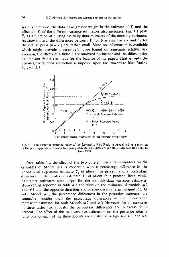
As b is increased, the data have greater weight in the estimate of Yr and the effect on yI of the different variance estimators also increases. Fig. 4.1 plots YI as a function of b using the daily data estimates of the monthly variances. As shown there, the differences between YI for b as small as six and YI for the diffuse prior (b= m) are rather small. Since no information is available which might provide a meaningful upperbound on aggregate relative risk aversion, the effects of a finite b are analyzed no further and the diffuse prior assumption (b = m ) is made for the balance of the paper. That is, only the non-negativity prior restriction is imposed upon the Reward-to-Risk Ratios, I$ j=l,2,3.

MODEL I : a(l)-r(t) = Y rr*(t)

0, = Least-Squares Estimate

7, = Prior Expected Value

VI OO

I I I I I I I I I I I I b I 2 3 4 5 6

Prior Upper- Bound RestrIctIan on the Reward-to-Risk Ratto

Fig. 4.1. The posterior expected value of the Reward-to-Risk Ratio in Model # 1 as a function of the prior upper-bound restriction using daily data estimates of monthly variance: July 1962 to

June 1978.

From table 4.1, the effect of the two different variance estimators on the

estimates of Model # 1 is moderate with a percentage difference in the unrestricted regression estimate yr of about five percent and a percentage difference in the posterior estimate YI of about four percent. Both model parameter estimates were larger for the monthly-data variance estimates. However, as reported in table 4.2, the effect on the estimates of Models #2 and # 3 is in the opposite direction and of considerably larger magnitude. As with Model # 1, the percentage differences in the posterior estimates are somewhat smaller than the percentage differences in the unrestricted regression estimates for both Models # 2 and # 3. However, for all estimates in these latter two models, the percentage differences are in excess of 30 percent. The effect of the two variance estimators on the posterior density functions for each of the three models are illustrated in figs. 4.2, 4.3, and 4.4.

Table 4.2

The effect of daily data versus monthly data estimates of variance on different models estimates with non-negative restriction only; July 1962 to June 1978.

Model #l: z(t)-t(t)= Y,d(t)

Monthly data estimates of variance 0.3482 1.5914 2.1180 Daily data estimates of variance 0.3733 1.5181 2.0341 Percentage difference - 6.72 “/A 4.83 :I; 4.12 9;

Mode1 #2: u(t)-r(t)=Y,o(t)

Monthly data estimates of variance 192 0.1123 0.1214 Daily data estimates of variance 192 0.1806 0.1818 Percentage difference 0 ‘, - 31.82 “/A - 33.22 4;

Model #3: a(r)-r(t)=Y,

Monthly data estimates of variance Daily data estimates of variance Percentage difference

Q: 9, Y3(b= x)

172185 0.0052 o.Oc53 221708 0.0082 0.0083 - 22.34 “/:, - 36.59 “/A - 35.37 o0

“Yi=Reward-to-Risk Ratio for Model #j, j=1,2,3. ~+x:[B~(t)]~-j. 3 = Unrestricted least-squares estimate of q. 5 = Expected value of q using the posterior distribution based upon a uniform prior

distribution on the interval [0, b].

DAILY ESTIMATE OF MONTHLY VARIANCE

VI = Postermr Expected Value

unbform Pr10r on [O, m)

0 I 2 3 4 5 6 Reword to Risk Ratio

MONTHLY ESTIMATE OF MONTHLY VARIANCE

Reword-to-Risk Ratlo

Fig. 4.2. The effect of different variance estimators on the posterior density function for the Reward-to-Risk Ratio in Model # 1; July 1962 to June 1978.

341


DAILY ESTIMATE OF MONTHLY VARIANCE

y* = Posterior Expected Value

Uniform Prior an [O,ID)

Reword-to- Risk Ratio

MONTHLY ESTIMATE OF MONTHLY VARIANCE

Reword-to-Risk Ratio

Fig. 4.3. The effect of different variance estimators on the posterior density function for the Reward-to-Risk Ratio in Model #2; July 1962 to June 1978.

While these brief comparisons cannot be considered an analysis of the effects of measurement error in the variance estimates, they do serve as a warning against attaching great significance to the point estimates of the models.

From table 4.2, it appears that for this period, the prior non-negativity restriction is important only for Model # 1 where for the same variance estimate, the percentage difference between YI and PI is approximately 25 percent. The differences between the posterior estimate and the unrestricted regression estimate for Model # 2 and Model # 3 are negligible. This result is further illustrated by inspection of the shapes and domains of the posterior density functions as plotted in figs. 4.2, 4.3 and 4.4.

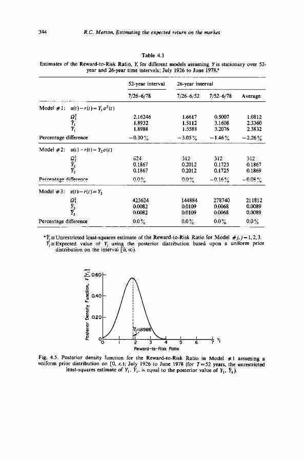
To further investigate the importance of the prior non-negativity restriction, the difference between the posterior and unrestricted regression estimates are examined for fifty-two years of data from July 1926 to June 1978. These estimates are presented in table 4.3 for both T=52 years and T =26 years. As inspection of this table immediately reveals, the percentage differences between % and 3 are negligible for all three models with T=52, and for Models # 2 and #3 with T=26. For Model # 1 with T=26, the


m DAILY ESTIMATE OF MONTHLY VARIANCE

v3 = Posterior Expected Value

of Y3

lhform Puor on [0, (D)

.h 50 -

a

0, = Least-Squares Estimate of Y3

b L o- \ L 0.0 0.0050 OOlOO 0.0150 0.0200 0.0250 ’ Y3 0.0500


? y 200

c^ 0 .$ 150

MONTHLY ESTIMATE I= OF MONTHLY VARIANCE

~l$Jy~ , ) ( ] y3

0.0 0.0050 01)tOO 0.0150 0.0200 00250 0.03oo Reward-to-Risk Rotio

Fig. 4.4. The effect of different estimators on the posterior density function for the Reward-to-Risk Ratio in Model # 3; July 1962 to June 1978.

differences are small with an average about half of that found in the previous analysis from 1962-1978. As before, the posterior density functions for each of the models with T=52 are plotted in figs. 4.5, 4.6, and 4.7. By the assumption that the 5, j = 1,2,3, are constant over such a long time period, the number. of observations N is quite large (624 for T=52 and 312 for T = 26). Given the previously-demonstrated asymptotic convergence of ?+ 5 for large N, these findings were not entirely unexpected. However, if shorter time intervals over which Ij is assumed to be constant are chosen, then the differences between %-and 5 are not negligible.

In table 4.4, the different model estimates of the Reward-to-Risk Ratios are presented for T= 13 years (with N = 156). The average percentage difference between 5 and q for the four 13-year time periods ranged from a high of 28 percent for Model # 1 to a low of 6 percent for Model # 3 with Model #2 in ‘the middle at a 12 percent difference. However, the’percentage differences for each of the time periods are more important than the average since by hypothesis, the 5 can only be estimated using 13 years of data.


Table 4.3

Estimates of the Reward-to-Risk Ratio, x for different models assuming Y is stationary over 52- year and 26-year time intervals; July 1926 to June 1978.”

52-year interval

7126-6178

26-year interval

7126-6152 7J52-6178 Average

Mode1 #l: a(t)-r(t)=Y,u’(t)

$

2

Percentage difference

2.16246 1.6617 0.5007 1.0812

1.8932 1.8988 1.5112 1.5588 3.1608 3.2076 2.3360 2.3832

-0.30% - 3.05 % -1.46% -2.26%

Model #2: a(t)-r(t)=Y,a(t)

?: Y -2 r,


624 312 312 312 0.1867 0.2012 0.1723 0.1867 0.1867 0.2012 0.1725 0.1869

0.0 y0 0.0% -0.16% -0.08%

Model #3: a(t)-r(t)= Y,

0: 3 t 3


423624 144884 278740 211812 0.0082 0.0109 0.0068 0.0089 0.0082 0.0109 0.0068 0.0089

0.0% 0.0% 0.0% 0.0%

‘3 c Unrestricted least-squares estimate of the Reward-to-Risk Ratio for Model #j, j = 1,2,3. 5~ Expected value of 3 using the posterior distribution based upon a uniform prior

distribution on the interval [0, co).

I I I c 4 5 6 77

Reward-to-Risk Ratio

Fig. 4.5. Posterior density function for the Reward-to-Risk Ratio in Model # 1 assuming a uniform prior distribution on [0, r); July 1926 to June 1978 (for T=52 years, the unrestricted

least-squares estimate of Y,, %‘, . is equal to the posterior value of I’,, U, ).


>-N t;’ 10.0 -

s ‘Z g 7.5-

I=

f 5.0 -

0’ 5 2.5 - j z a. 0.0. I I

0.0 0.10 0.20 0.30 040 0.50 0.60 vz

Reword- to- Risk Rotto

Fig. 4.6. Posterior density function for the Reward-to-Risk Ratio in Model #2 assuming a uniform prior distribution on [O, I)); July 1926 to June 1978 (for T=52 years, the unrestricted

least-squares estimate of Y2, Yz is equal to the posterior expected value of Yz, Y,).

g 300 t-

r t z g IOO-

B 5

B 0 I I ’ 0.0 0.0050 0.0100 Ox)150 0.0200 0.0250 W3CG y3


Fig. 4.7. Posterior density function for the Reward-to-Risk Ratio in Model #3 assuming a uniform prior distribution on [0, XI); July 1926 to June 1978 (for T=52 years, the unrestricted

least-squares estimate of YS, YS, is equal to the posterior expected value of Y3, Y,).

In the 196551978 period, the percentagk differences between the posterior estimate and the unrestricted regression estimate are substantial for all three models. This was a period with a number of large negative realized excess returns on the market, and this is precisely the type of period in which the prior non-negativity restriction can be expected to be important. The periods 1939-1952 and 1952-1965 did not have these large negative realized excess returns and correspondingly, the non-negativity restriction was (ex post) unimportant. The period 1926-1939 appears to be different from the other three in that the effect of the non-negativity restriction is quite large for Model # 1; small for Model # 2; and negligible for Model # 3. However, the results from this period are consistent with the oth.ers. This was a period of

346 R.C. Merton, Estimating the expected return on the murket

Table 4.4

Estimates of the Reward-to-Risk Ratio, x for different models assuming Y is stationary over 13- year time intervals; July 1926 to June 1978.

71266139 7139-6152 7152-6165 7165-6178 Average

Model #I: z(t)-r(t)=Y’,u*(t)

:: <

0.628 1.3344 1 0.3273 5.1114 0.1936 7.5772 0.3777 0.3072 0.5406 3.4236 0.9747 5.1211 7.5807 1.5858 3.8156

Percentage difference - 35.56 % -0.19% -0.05 7; -76.180/A -28.00>;

Model #2: a(t)-r(t)= Y2u(t)

n: 156 156 156 156 156 YZ 0.1569 0.2454 0.2982 0.0464 0.1867 2 0.1617 0.2457 0.2983 0.0840 0.1974

Percentage difference - 2.97 7; -0.12% - 0.03 y0 -44.76% - 11.97 ;:

Model #3: a(t)-r(t)=Y,

9: 44439 100445 164110 114630 105906

Y $

0.0146 0.0092 0.0096 0.0029 0.0091

3 0.0146 0.0092 0.0096 0.0038 0.0093

Percentage difference 0.0 “/; 0.0 U/0 0.0 % - 23.68 7; - 5.92 ;L

‘?.= Unrestricted least-squares estimate of the Reward-to-Risk Ratio for Model #j, j = 1,2,3. I$ Expected value of 5 using the posterior distribution based upon a uniform prior

distribution on the interval [O, co).

both large positive and negative realized excess. returns with both large changes in variance and large variances especially in the early 1930’s when the market had a large negative average excess return. From the regression estimators, (2.2), & has in its numerator the unweighted average of the (logarithmic) realized excess returns. pZ has in its numerator the weighted average of these excess returns where the weights are such that each excess return is ‘deflated’ by that month’s estimate of the standard deviation. That is, unlike $‘I in which each observed excess return has the same weight, p2 puts more weight on observed excess returns which occur in lowerlhan- average-standard-deviation months and less weight on those that occur on higher-than-average-standard-deviation months. Inspection of the regression estimator for Model #3 will show that the weighting of the realized excess returns 1s similar to that of $‘Z except the effect is more pronounced because each month’s return is divided by that month’s variance. Hence, in a period such as the early 1930’s when, ex post, large negative excess returns occur in months where the variance is also quite large, the differences between pj and $ will be largest in Model # 1 and smallest in Model # 3. Of course, just the opposite effect will occur in periods when, ex post, either large negative

R.C. Merton, Esrimuting the expected return on the market 341

excess returns &cur in months when the variance is small, or more likely, large positive excess returns occur in months when the variance is large and a number of negative excess returns occur in months when the variance is small.

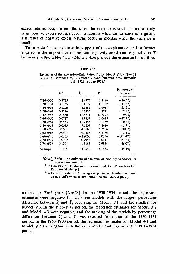
To provide further evidence in support of this #explanation and to further underscore the importance of the non-negativity constraint, especially as T becomes smaller, tables 4Sa, 4Sb, and 4.5~ provide the estimates for all three

Table 4.5a

Estimates of the Reward-to-Risk Ratio, Y,, for Model # 1: a(t)-r(t) = Y,a*(t), assuming Y, is stationary over four-year time intervals;

July 1926 to June 1978.


l/266/30 0.1785 2.4118 3.1184 - 20.5 % l/3&6/34 0.8365 -0.1097 0.8337 - 113.2 % 7/346/38 0.2216 1.9389 2.6017 -25.5% l/38-6/42 0.2226 0.2156 1.1121 -81.8% l/42-6/46 0.0860 12.6511 12.6525 0.0 7; l/4&6/50 0.0181 1.9159 3.6625 - 47.1 y0 l/50-6/54 0.0553 12.2185 12.2459 -0.2% l/546/58 0.0685 1.6509 7.8610 -2.7% l/58&6/62 0.0607 4.3146 5.3906 -2o.o”/; 1162-6166 0.0507 9.0518 9.2186 -2.47; 7/666/10 0.0863 - 2.2060 2.0534 - 201.4 7; 7/l&6/14 0.0909 0.9986 3.0443 - 67.2 7; l/146/18 0.1204 1.6183 2.9964 -46.0%

Average 0.1664 4.0566 5.1932 -49.3 y0

‘@=~:“B’(f), the estimate of the sum of monthly variances for four-year time intervals.

Y, = Unrestricted least-squares estimate of the Reward-to-Risk Ratio for Model # 1.

Y, ~Expected value of Y, using the posterior distribution based upon a uniform prior distribution on the interval [0, x;).

models for T=4 years (N=48). In the 193&1934 period, the regression estimates were negative for all three models with the largest percentage ‘difference between q and q occurring for Model # 1 and the smallest for Model # 3. In the 193%1942,period, the regression estimates for Model #2 and Model #3 were negative, and the ranking of the models by percentage differences between $ and $ was reversed from that of the 193&1934 period. In the 19661970 period, the regression estimates for Model # 1 and Model #2 are negative with the same model rankings as in the .1930-1934 period.

Table 4.5b

Estimates of the Reward-to-Risk Ratio, Y2, for Model #2: a(f)--(t) = Y,a(t), assuming Y, is stationary over four-year time intervals;

July 1926 to June 1978.

r;

Percentage dilTerence

7/2&6/30 7/3&6/34 71346138 7/38-6142 7142-6146 7/466/50 7/5&6/54 7154-6158 7158-6162 7162-6166 7/666/70 7/7@-6/74 71746178

Average

48 0.2658 0.2768 48 - 0.0084 0.1122 48 0.2549 0.2675 48 -0.1288 0.0790 48 0.5509 0.5510 48 0.1206 0.1715 48 0.4109 0.4119 48 0.2954 0.3027 48 0.2171 0.2370 48 0.3293 0.3336 48 -0.0355 0.1032 48 0.0653 0.1424 48 0.0901 0.1547

48 0.1867 0.2418

-4.0% - 107.5 7;

-4.7% -263.0%

0.0 “/: - 29.7 % -0.2% -2.4% - 8.4 y0 -1.37;

-134.4% -54.1% -41.8%

-50.1%

‘$=N =number of months in a four-year time interval. Y, G Unrestricted least-squares estimate of the Reward-to-Risk

Ratio for Model #2. T;=Expected value of Y2 using the posterior distribution

based upon a uniform prior distribution on the interval

CO, =).

Table 4.5~

Estimates of the Reward-to-Risk Ratio, Y,, for Model #3: a(t) -r(t)= Y3, assuming YS is stationary over four-year time

intervals; July 1926 to June 1978.

E, r;


7/2&6/30 22344 0.0165 0.0167 7/3&6/34 4091 -0.0015 0.0119 7134-6138 16124 0.0183 0.0185 7138-6142 19633 -0.0149 0.0026 7142-6146 29693 0.0222 0.0222 7/466/50 33517 0.0062 0.0075 7/5&6/54 47626 0.0126 0.0126 71546158 35062 0.0111 0.0113 7/58-6162 43347 0.0084 0.0088 7162-6166 73342 0.0088 0.0089 7/666/70 30920 0.0014 0.0051 7170-6174 35864 0.0031 0.0056 7/746/78 32059 0.0029 0.0057

Average 32586 0.0073 0.0106

- 1.2% - 112.6%

-1.1% -673.1%

0.0% - 17.3 7;

0.0 % -1.8% -4.5 % -1.1%

- 72.5 % -44.6% -49.1%

- 75.3 %

“0: = 1:” [l/t?(t)], the sum of the reciprocal of the estimates of monthly variances for four-year time intervals.

2~ Unrestricted least-squares estimate of the Reward-to-Risk Ratio for Model #3.

Y,=Expected value of Ya using the posterior distribution based upon a uniform prior distribution on the interval

CO, 3)). 348

R.C. Merton, Estimuting the expected return on the market 349

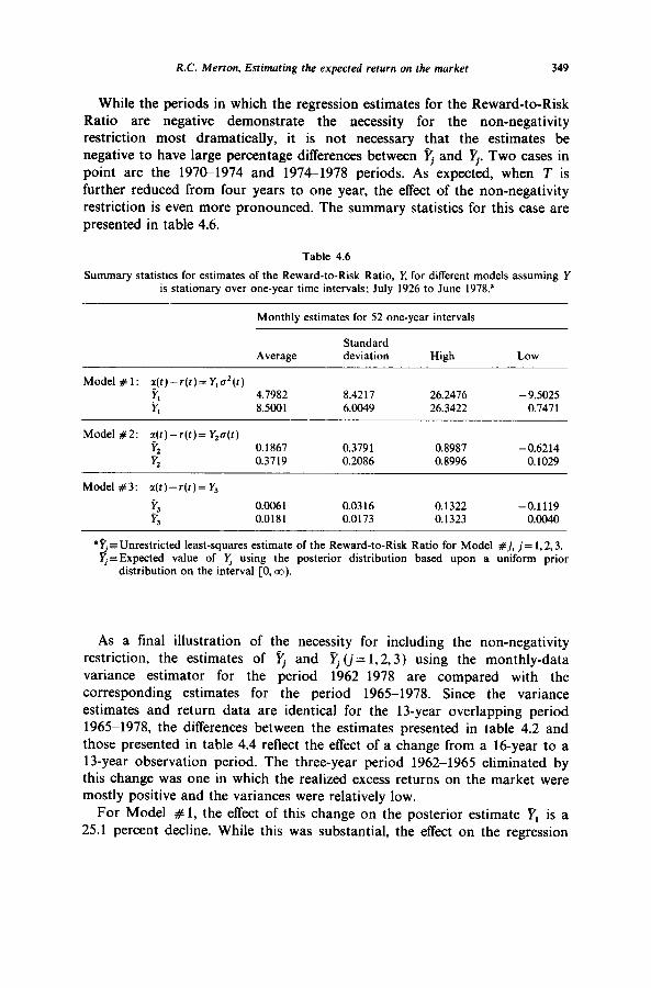
While the periods in which the regression estimates for the Reward-to-Risk Ratio are negative demonstrate the necessity for the non-negativity restriction most dramatically, it is not necessary that the estimates be negative to have large percentage differences between Fj and Yj. Two cases in point are the 1970-1974 and 1974-1978 periods. As expected, when T is further reduced from four years to one year, the effect of the non-negativity restriction is even more pronounced. The summary statistics for this case are presented in table 4.6.

Table 4.6

Summary statistics for estimates of the Reward-to-Risk Ratio, Y, for different models assuming Y is stationary over one-year time intervals; July 1926 to June 1978.’

Monthly estimates for 52 one-year intervals

Standard Average deviation High Low

Model #l: gt)-r(f)=Y,c’(t)

Y; 4.7982 8.5001 6.0049 8.4217 26.2476 26.3422 -

9.5025 0.7471

Model #2: a(t)-r(t)= Y+(t) % 0.1867 0.3791 0.8987 -0.6214 r, 0.3719 0.2086 0.8996 0.1029

Model #3: a(t)-r(t)=Y,

t G

0.006 1 0.0316 0.1322 -0.1119

3 0.0181 0.0173 0.1323 0.0040

“3 EUnrestricted least-squares estimate of the Reward-to-Risk Ratio for Model #j, j= 1,2,3. I;-~Expected value of I; using the posterior distribution based upon a uniform prior

distribution on the interval [0, 03).

As a final illustration of the necessity for including the non-negativity restriction, the estimates of 5 and q (j= 1,2,3) using the monthly-data variance estimator for the period 1962-1978 are compared with the corresponding estimates for the period 196551978. Since the variance estimates and return data are identical for the 13-year overlapping period 1965-1978, the differences between the estimates presented in table 4.2 and those presented in table 4.4 reflect the effect of a change from a 16-year to a 13-year observation period. The three-year period 1962-1965 eliminated by this change was one in which the realized excess returns on the market were mostly positive and the variances were relatively low.

For Model # 1, the effect of this change on the posterior estimate YI is a 25.1 percent decline. While this was substantial, the effect on the regression

350 R.C. Merton, Estimuting the expected return on the murket

estimate was much greater with a decline in %‘i of 76.3 percent. The effect on the other model estimates is similar. For Model #2, the posterior estimate YZ changes by 30.8 percent with a corresponding change in FZ of 58.7 percent. For Model #3, the change in Y3 is 28.3 percent and the change in Pa is 44.2 percent.

The substantial percentage change in both the 6 and 3 estimates from a relatively small change in the observation period illustrates the general difficulty in accurately estimating the parameters in an expected return model and underscores the importance of using as long a historical time series as is available. However, very long time series are not always available, and even when they are, it may not be reasonable to assume that the parameters to be estimated were stationary over that long a period. Therefore, given the relative stability of the Yj estimator by comparison with %, it appears that the non-negativity restriction should be incorporated in the specification of any such expected return model.

Having analyzed the empirical estimates of the Reward-to-Risk Ratios, we now examine the properties of the expected excess returns on the market implied by each of these models. For this purpose, it is assumed that the 5 (j= 1,2,3) were constant over the entire period 19261978, and therefore, T equals 52 years. Or course, this assumption is certainly open to question. However, given the much-discussed problems with the variance estimators and the exploratory spirit with which this paper is presented, further refinements as to the best estimate of T are not warranted here. Moreover, as discussed in section 2, the current state-of-the-art model implicitly makes this assumption by using as its estimate of the expected excess return on the market, the sample average of realized excess returns over the longest data period available.

Using the estimated % and the time series of estimates for the market variances, monthly time series of the expected excess return on the market were generated for each of the three models over the 624 months from July 1926 to June 1978. As shown in figs. 4.5, 4.6, and 4.7, with T equal to 52 years, the posterior density functions for all three models are virtually symmetric and the differences between q and < are negligible.i6

The summary statistics for these monthly time series are reported in table 4.7 and they include the sample average, standard deviation and the highest and lowest values. Of course, the expected excess return estimate for Model #3 is simply a constant. In table 4.7, the same summary statistics are presented for the reulized excess returns on the market and for the realized returns on the riskless asset.

Inspection of table 4.7 shows that the average of the expected excess returns varies considerably across the three models. The ‘Constant-

16Hence, for T= 52 years, the monthly time series of expected excess returns using the unrestricted regression estimate would be identical to those presented here.

R.C. Merton, Estimctting the expected return on the murket 351


Preferences’ Model # 1 is the lowest with an average of 0.665 percent per month or, expressed as an annualized excess return, 8.28 percent per year. The ‘Constant-Price-of-Risk’ Model #2 is the highest with an annualized excess return average of 12.04 percent per year. The ‘Constant-Expected- Excess-Return’ Model #3 is almost exactly midway between the other two models with an annualized average of 10.36%. The sample average of the reulized excess returns on the market was 0.655 percent per month, or, annualized, 8.15 percent per year. This sample average is also the point estimate for the expected excess return on the market according to the state- of-the-art model.

Even with these large differences in the average estimates, it is unlikely that any of these models could be rejected by the realized return data. The variance of the unanticipated part of the returns on the market is much larger than the variance of the change in expected return. That is, the realized returns are a very ‘noisy’ series for detecting differences among models of expected return.

In examining the average excess returns in table 4.7, one might be tempted to conclude that Model # 1 ‘looks’ a little better because its average is so

close to the sample average of realized excess returns. However, as inspection of (2.2a) makes clear, the regression estimator ?i is such that this must always be the case when the variance estimator is of the type used here. This observation brings up an important issue with respect to estimates based upon the state-of-the-art model.

If the strict formulation of that model is that the expected excess return on the market is a constant or at least, stationary over time, then the least- squares estimate of that constant is given by %‘a in Model #3. However, from table 4.7, the annualized difference between p3 and the sample realized return average is 221 basis points. This difference is quite large when considered in the context of portfolio selection and corporate finance applications. The reason for the difference is that the sample average of realized returns is only a least-squares estimate if the variance of returns over the period is constant. If the variance is not constant, and it isn’t, then the

estimator should be adjusted for heteroscedasticity in the ‘error’ terms. This. is exactly what the estimator vJ does. Of course, the sample average of realized returns is a consistent estimator and the measurement error problem in the variance estimates rule out formal statistical comparison. However, the large difference reported here should provide a warning against neglecting the effects of changing variance in such estimations and simply relying upon ‘consistency’ even when the observation period is as long as 52 years.

As mentioned, the sample average of the realized returns will provide an efficient estimate of the average expected return if Model # 1 is the correct specification. However, even if that is the belief, then for capital market and corporate finance applications, ?, times the estimate of the current variance


will provide a better estimate of the current expected excess return than the state-of-the-art model because it takes into account the current level of risk associated with the market.

A similar argument applies to using the ratio of the sample average of the realized excess returns to the sample standard deviation for estimating the Price of Risk under the hypothesis that it is constant, or at least, stationary over time. From table 4.7, using the realized return statistics, the estimate of the Price of Risk is 0.114 per month whereas from table 4.3, the least-squares estimate & which takes into account the changing variance rates is 0.1867 per month. Again, this difference is quite large.

Table 4.8

Successive four-year average monthly variance estimates for the return on the market; July 1926 to June 1978.

Dates Average monthly variance”

Percentage change from previous period

7/2&6/30 0.003719 7/3%6/34 0.017427 368.59 7; 7/346/38 0.004742 - 72.79 “/;, 7138-6142 0.004638 -2.197; 7142-6146 0.001792 -61.36”/; 71466150 0.001640 - 8.48 ‘:; 7/5&6/54 0.001152 - 29.76 “/, 7154-6158 0.001427 23.87 ‘;:, 715%6162 0.001265 -11.35% 7162-6166 0.001056 - 16.52 “/:, 71666170 0.001798 70.27 “/:, 7/7&6/74 0.001894 5.34 “/, 71746178 0.002508 32.42 “/,

Average 0.003467

aThe four-year average monthly variance was computed for each non-overlapping four-year period by [cf!, S2(t)]/48 where (4.3) was used for the variance estimator B’(t).

To further underscore the importance of taking into account the change in the variance rate when estimating the expected return on the market, we close this section with a brief examination of the time series of market variance estimates. The average monthly variance rates for the market returns are presented in table 4.8 for the thirteen successive four-year periods from July 1926 to June 1978. Over the entire 52-year period, the average annual standard deviation of the market return was 20.4 percent. However, as is clearly demonstrated in table 4.8, the variance rate can change by a substantial amount from one four-year period to another, and it is significantly different from this average in many of the four-year periods.

J.F.E.-_B


It has frequently been reported that the market was considerably more volatile in the pre-World War II period than it has been in the post-war period. That observation is confirmed here with an average annual standard deviation of 27.9 percent for the period July 1926 to June 1946 versus 13.8 percent for the period July 1946 to June 1978. However, a significant part of this difference is explained by the extraordinarily large variance rates in the 1930-1934 period. Thus, if this period is excluded, then the average annual standard deviation for the other twelve four-year periods is 16.6 percent.

Because the state-of-the-art model assumes a constant variance rate, the large differences in variance rates among the various subperiods causes this model’s estimates to be quite sensitive to the time period of history used. So,

for example, if 1930-1934 is excluded, then the estimated Market Price of Risk based upon the other forty-eight years of data changes by 33 percent for the state-of-the-art model estimator. However, this same exclusion causes Model #2’s estimate, p2, to change by only 8 percent.

5. Conclusion

In this exploratory investigation, we have established two substantive results: First, whether or not one agrees with the specific way in which it was incorporated here, it has been shown that in estimating models of the expected return on the market, the non-negativity restriction on the expected excess return should be explicitly included as part of the specification. Second, because the variance of the market return changes significantly over time, estimators which use realized return time series should be adjusted for

heteroscedasticity. As suggested by the empirical results presented here, estimators based upon the assumption of a constant variance rate, although consistent, can produce substantially different estimates than the proper weighted least-squares estimator even when the time series are as long as fifty years. As demonstrated by the analysis of Model #3, these conclusions apply even if the model specification is such that the expected excess return does not depend upon the level of market risk.

There are at least three directions in which further research along these lines could prove fruitful. First, because the realized return data provide ‘noisy’ estimates of expected return, it may be possible to improve the model estimates by using additional non-market data. Examples of such other data are the surveys of investor holdings as used in Blume and Friend (1975): the surveys of investor expectations as used in Malkiel and Cragg (1979); and corporate earnings and other accounting data as used in Myers and Pogue (1979). Because these types of data are not available with the regularity and completeness of market return data, it may be more appropriate to include them through a prior distribution rather than as simply additional variables in a standard time series regression analysis. If a prior distribution is to be

R.C. Merton, Estimcrting the expected return on the market 355

used to incorporate both these data and the non-negativity restriction, then the sensitivity of the model estimates to the particular distribution chosen warrants careful study.

A second direction is to employ a more sophisticated approach to the non- stationarity of the time series. Such an approach could be used to estimate the length of time over which it is assumed that the Reward-to-Risk Ratio can be treated as essentially constant (i.e., T). In the analysis presented here, the estimates of q for different T only used the data for the specific subperiod. So, for example, the Yj for the period 1930-1934 was computed using only the observed returns for 1930-1934. Clearly, better estimates could be obtained by including the pre-1930 observations as well. Therefore, for a given T, the estimates will be improved by developing a procedure for revising the prior distribution using ptrsr estimates of 5..

The third and most important direction is to develop accurate variance estimation models which take account of the errors in variance estimates. As previously discussed, such models have applications far broader than simply estimating expected returns. Such models should benefit from inclusion of both option price data and accounting data in addition to the past time series of market returns. Perhaps other market data such as trading volume may improve the estimates as well.

While there are obviously many problems to be overcome in both the estimation and testing of expected return models, it is hoped that this paper will stimulate further research effort and with it, some solutions to this

important problem.

Appendix A

Estimtrting the curiunce rnte from time series of retrlized returns

In the Introduction, it was claimed that the variance of returns can be estimated far more accurately from the available time series of realized returns than can the expected return. We now show that this claim is correct provided that market returns can be described by a diffusion-type stochastic process as in (2.5) and that the mean and variance of these returns are slowly-varying functions of time.

As discussed in detail in section 2 of the text, under the hypothesis that the mean and variance are slowly-varying functions of time, the true process for market returns can be approximated by assuming that p and G* are constants over (non-overlapping) time intervals of length /r where p is the expected logurithmic rate of return on the market per unit time and a2 is the variance per unit time. Suppose that the realized return on the market can be observed over time intervals of length A where A <h. Then n = h/A is the number of observations of realized returns over a time interval of length h.


So, for example, if h equals 1 month and A equals 1 day, then n equals 30 (neglecting weekends and holidays). Let X, denote the logarithmic return on the market over the kth observation interval of length A during a typical period of length h for k = 1,2,. . ., n. From (2.5), X, can be written as

X,=pA +a&~~, k=1,2 ,..., n, (A.1)

where the {Q}, k= 1,. .., n, are independent and identically distributed standard normal random variables.

From (A.l), the estimator for the expected logarithmic return, fi =[c; XJh, will have the properties that

and

ECPI =A

var [fi] = a2/h.

(A-2)

(A.3)

Note that the accuracy of the estimator as measured by var[F] depends only upon the total length of the observation period h and not upon the number of observations n. That is, nothing is gained in terms of accuracy of the expected return estimate by choosing finer observation intervals for the returns and thereby, increasing the number of observations n for a fixed value of h.

Consider the following estimator for the variance rate: g2 =[I; X,21/h. From (A.l), this estimator will have the properties that

(A.4)

and

(A.5)

Because the estimator for a2 was not taken around the sample mean fi. c?~ is biased as shown in (A.4). However, for large n, the difference between the sample second central and non-central moments is trivial. For example, typical values for ,u and tr2 in annual units would be 0.10 and 0.04, respectively. For daily observations, h/n will equal approximately l/360. Therefore, substituting into (A.4), we have that E(c?~) will equal 0.0400277 when the expectation of an unbiased estimator is 0.04. Even for monthly observations with h/n equal to 12, E(82)=0.0408333 and the bias of this estimator is still trivial.

The advantage of this estimator is that the variance can be estimated without knowing or even having an estimate of the mean ,u. It also, of course, saves one degree of freedom. Thus, for stock return data and


observation intervals of a month or less, the bias from a non-central

estimator of the variance can be neglected. More important than the issue of bias is the accuracy of the estimator. As

inspection of (A.5) quickly reveals, var(k2) does depend upon the number of

observations n for a fixed h, and indeed, to order l/n, it depends only upon the number of observations. Thus, unlike the accuracy of the expected return estimator, by choosing liner observation intervals d, the accuracy of the variance estimator can be improved for a fixed value of h.

To further emphasize the point, consider the extreme case where both the mean and variance are constant for all time. The accuracy of the expected value estimator will depend only on the total length of calendar time for which return data are available (e.g., 52 years). However, the accuracy of the variance estimator will depend critically on whether these data are available annually, quarterly, monthly, or daily. The standard deviation of the variance estimate using annual data will be approximately nineteen times larger than the standard deviation of the estimate using daily data over the same calendar period. Since neither the mean nor the variance are constant for anything like this length of calendar time, the practical advantage of the variance estimator’s accuracy depending upon n rather than h is that a reasonably accurate estimate of the variance rate can be obtained using daily data while the estimates for expected return taken directly from the sample will be subject to so much error as to be almost useless. Additional discussion on these points can be found in Merton (1976, pp. 336-339).

In the theoretical limit of continuous observation, n goes to infinity for any finite h, and therefore, the variance rate could in principle be estimated without error for any finite interval. However, in practice, the choice of an ever-shorter observation interval introduces another type of error which will ‘swamp’ the benefit of a shorter time interval long before the continuous limit is reached. This error is caused by not knowing the exact length of time between successive trades. For example, suppose that the closing price of a stock as reported in the newspaper was not the result of trade at 4:00 p.m., but rather the result of a (last) trade which occurred at 3:00 p.m. If A is one week and if the last trade the previous week did occur at 4:00 p.m., then the observed price change occurred over a 167 hour interval and not a 168 hour interval as assumed. While this actual shorter time interval will cause an underestimate of the variance rate, the magnitude of the error is only 0.6 percent. However, suppose that A is the six-hour interval from the 10:a.m. opening to the same day 4:00 p.m. closing. Then, even if the first trade occurs at 10:00 a.m., the actual interval for the observed price change is live hours and not six, and the magnitude of the error in the variance rate would be 16.7 percent. Of course, if the first trade actually took place at 1l:OO a.m., then the error would be 33.3 percent. Thus, the ‘true’ time interval between trades is a random variable.


For actively-traded stocks and a A of the order of a week or more, this error will generally have a negligible effect on the variance estimates. However, for daily observations, it can have a non-negligible effect for individual stocks, and it will definitely be important for a large portfolio of stocks such as the NYSE index. It is more important for a large portfolio because it is likely that a significant number of the stocks in the portfolio will not have their last trade near the closing time. Since the closing value of the index is computed using the last traded prices and since stocks tend to be contemporaneously positively correlated with one another, the observed daily changes in the index will exhibit positive serial correlation. This positive correlation is not ‘real’ in the sense that one could make money trading in the individual stocks contained in the index because at 4:00 p.m., trades could not have been executed at these last (and earlier) prices. However, if no adjustment is made for this ‘non-trading’ effect, then the sum of squared daily logarithmic changes in the index will produce a significantly biased-low estimate of the variance rate.

A method for correcting for this problem is as follows: Let Xii denote the observed change in the index as contrasted with X, in (A.l) which is the true change. Since it is not known for how many days this ‘non-trading’ effect lingers, it was simply assumed that after three days, there is no effect. A model specification which captures this non-trading effect is given by

where Os6,51, j=O,1,2,3, and &=l-6,-S,-6,. From (A.6), we have that

(A-7)

Comparing (A.7) with (A.4) confirms that the unadjusted estimator is biased low for the posited restrictions on the hi. If the (Sj} were known, then (neglecting the p2 A term) there is a simple adjustment: Namely, divide the observed sum of squares by [E= ,, sf]. Of course, they are not known, and therefore, must be estimated.

In section 4, daily data are used in one of the variance estimators for the period July 1962 to June 1978. To adjust the estimates for serial correlation, the dj were estimated using nonlinear procedures on the following equation:

X,=A+BX,_, +B2Xk_2 +B3&_3. (44.8)

R.C. Merton, Estimuting the expected return on the market 359

From (A.6) and (A.8), we have that

B=[6, th,b, tb2d3]/[1 +df tb: t&i],

B2 =[& t6,bJ/[l ts: td2, td:],

B3=b3/[1 +bf t(s; tig].

(A.9)

In the sample period, A =0.0002 with standard error 0.0001 and B=0.2106 with standard error 0.0114. The corresponding values for bj from (A.9) are 6, =0.734, d, =0.221, 6, =0.045, d3 =O.OlO, xj”=,,6f =0.5854, and this was the number used to adjust for non-trading in the daily data variance estimator in the text. Adjustments were also made for non-trading days (i.e., weekends and holidays) by dividing the ‘daily’ returns by the square root of the number of days between trades.

Appendix B

The posterior distributiorl for q

In section 3, we have from (3.1) that

X’(r)= q[a(r)]2-’ te(t), j=l,2,3, t=l,...,N. (B.1)

where the prior density for q is uniform with f( Yj) = l/b for Oj q 5 b and zero, otherwise. Because the {s(t)) are independently and identically distributed standard normal, the joint density for X’( 1 ), . . ., X’(N), conditional on knowing I;. is given by

g[X’(l),..., X’(N)( YJ =exp i

-+i [X’(t)-- ~C~(t)12-‘12 1,

I (27r)N’2 1

=e -fQjexp[-+L?~(1;--E,.)2]/(27c)N/2,

(B.2)

where

and Qf and i.j are as defined in (3.4a) and (3.4b).

360 R.C. Merton, Estimnting the expected return on the market

By Bayes Theorem, the posterior density for 5 given X’(l), . . .,X’(N) can be written as, j = 1,2,3,

F[IjX’(l),..., X’(N )I = Cd ‘1 Yjllb} I {i gC * 1 Yjl dYj/b} i 0

(B.3)

By the change in the variable of integration u zQj[yj-lj], we have that

=2n{@(Pj)-@(?j)}lQjzi, (B.4)

where fj=Qj(b -Aj) and qj- -;ljQj. By combining (B.3) and (B.4), we have expression (3.3) for F[YjI .] given in the text.

To determine q =E[ q 1 c, Szf ; b], we simply multiply F[ q 1 .] by 5 and integrate from q = 0 to 5 = b, and note that yj = ,Ij.

References

Breeden, D., 1979, An intertemporal asset pricing model with stochastic consumption and investment opportunities, Journal of Financial Economics 7, Sept., 265-296.

Black, F., 1976, Studies of stock price volatility changes, Proceedings of the 1976 Meetings of Business and Economic Statistics Section, American Statistical Association, 177-181.

Black, F. and M. Scholes, 1973, The pricing of options and corporate liabilities, Journal of Political Economy 81, May-June, 6377659.

Black, F., M.C. Jensen and M. Scholes, 1972, The capital asset pricing model: Some empirical tests, in: M.C. Jensen, ed., Studies in the theory of capital markets (Praeger, New York).

Blume, M. and I. Friend, 1975, The asset structure of individual portfolios and some implications for utility functions, Journal of Finance 30, May, 585603.

Cox, J., J. Ingersoll and S. Ross, forthcoming, A theory of the term structure of interest rates, Econometrica.

Fama, E. and J. MacBeth, 1974, Tests of the multi-period two-parameter model, Journal of Financial Economics 1, May, 43-66.

Fama, E. and G. Schwert, 1977a, Human capital and capital market equilibrium, Journal of Financial Economics 4, Jan., 95-125.

Fama, E. and G. Schwert, 1977b, Asset returns and inflation, Journal of Financial Economics 5, Nov., 115-146.

Friend, I. and M. Blume, 1970, Measurement of portfolio performance under uncertainty, American Economic Review 60, 561-575.

Ibbotson, R. and R. Sinquefield, 1976, Stocks, bonds, bills, and inflation: Year-by-year historical returns (19261974), Journal of Business 49, Jan., 1147.

Ibbotson, R. and R. Sinquelield, 1977, Stocks, bonds, bills, and inflation: The past (19261976) and the future (197772000) (Financial Analysts Research Foundation, Charlottsville, VA).


Ibbotson, R. and R. Sinquelield, 1979, Stocks, bonds, bills, and inflation: Historical returns (1926-1978) (Financial Analysts Research Foundation, Charlottesville, VA).

Jensen, MC., 1972, Capital markets: Theory and evidence, Bell Journal of Economics and Management Science 3, 357-398.

Latane, H. and R. Rendleman, 1976, Standard deviations of stock price ratios implied in option prices, Journal of Finance 31, May. 369-381.

Lintner, J., 1965, The valuation of risk assets and the selection of risky investments in stock portfolios and capital budgets, Review of Economics and Statistics 47, 13-37.

Long, J.B., 1974, Stock prices, inflation, and the term structure of interest rates, Journal of Financial Economics 1, July, 131-170.

Malkiel, B. and J. Cragg, 1979, Expectations and the valuation of shares, Mimeo. Merton, R.C., 1971, Optimum consumption and portfolio rules in a continuous time model,

Journal of Economic Theory 3, Dec., 373413. Merton, R.C., 1973, An intertemporal capital asset pricing model, Econometrica 41, Sept., 867-

887. Merton, R.C., 1976, The impact on option pricing of specification error in the underlying stock

returns, Journal of Finance 31, May, 333-350. Merton, R.C., forthcoming a, On the mathematics and economic assumptions of continuous-

time models, in: W.F. Sharpe, ed., Financial economics: Essays in honor of Paul Cootner (North-Holland, Amsterdam).

Merton, R.C., forthcoming b, On the microeconomic theory of investment under uncertainty, in: K. Arrow and M. Intriligator, eds., Handbook of mathematical economics, Vol. II (North- Holland, Amsterdam).

Mossin, J., 1966, Equilibrium in a capital asset market, Econometrica 35, 768-783. Myers, S.C. and G. Pogue, 1979, Measuring expected rates of return, risk premiums, and the

market price of risk, Mimeo. Officer, R.R., 1973, The variability of the market factor of the New York stock exchange,

Journal of Business 46, July, 434453. Rosenberg, B., 1972, The behavior of random variables with non-stationary variance and the

distribution of security prices, Graduate School of Business Administration working paper no. 11, Dec. (University of California, Berkeley, CA).

Ross, S., 1976, Arbitrage theory of capital asset pricing, Journal of Economic Theory 8. Rothschild, M. and J. Stiglitz, 1970, Increasing risk I: A definition, Journal of Economic Theory

2, 225-243. Schmalensee, R. and R. Trippi, 1978, Common stock volatility expectations implied by option

premia, Journal of Finance 33, March, 129-147. Sharpe, W., 1964, Capital asset prices: A theory of market equilibrium under conditions of risk,

Journal of Finance 19, Sept., 425442. Treynor, J. and F. Black, 1973, How to use security analysis to improve portfolio selection,

Journal of Business 46, Jan., 66-86.

J.F.E.- C

ON ESTIMATING THE EXPECTED RETURN ON THE...

Documents

Transcript of ON ESTIMATING THE EXPECTED RETURN ON THE...