On data assimilation and ENSO dynamical prediction

IRI – June 2004

On data assimilation and ENSO dynamical prediction

Eli Galanti

IRI - Columbia University

With:

IRI - Mike Tippet, Steve Zebiak, Dave DeWitt

GFDL - Andrew Wittenberg, Matt Harrison, Tony Rosati

GFSC: Michele Rienecker and others

Outline

• The new IRI ocean data assimilation system

• ENSO forecast experiments and the role of stochastic forcing

• The TAO array east/west experiment

• Measuring impact of observing system’s lifetime in a simple model

• Develop local capability at IRI to initialize and forecast the tropical global SST.

• Global domain, medium resolution (Tropics focused)

• GFDL 3Dvar data assimilation scheme

• Run in real-time – update every month

• Initialization and forecast experiments with both hybrid and coupled GCM forecast systems.

IRI new ocean initialization and forecast system(In collaboration with GFDL)

The ocean model setup

• GFDL new GCM (MOM4)

• Mixing: vertical – KPP, horizontal – constant.

• Partial cells, free surface, etc…

• Surface forcing (NCEP reanalysis-2):

Monthly mean winds (NCEP anomalies + SSMI climatology)

Climatological heat fluxes

Monthly mean Reynolds SST

The ocean data assimilation (ODA)

• GFDL 3Dvar (sequential)

• Assimilate TAO, XBT, ARGO

• Run 1980 – present

• Experiment with strength of data assimilation.

• Future plans: improve assimilation by incorporating information on model dynamics.

comparison to NCEP ocean analysis (currently used at IRI to initialize forecasts) – heat content (J/m2/1.e9)

NCEP IRI

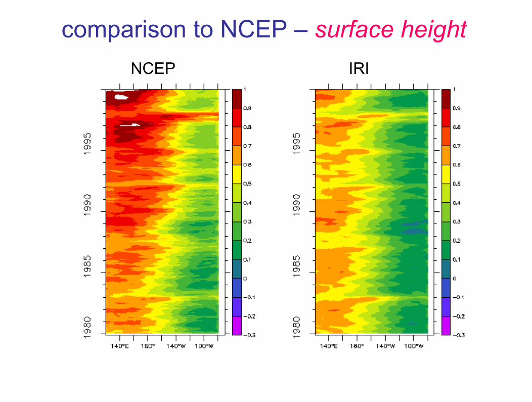
comparison to NCEP – surface heightNCEP IRI

comparison to NCEP – temp 140W

NCEP

IRI

dept

hde

pth

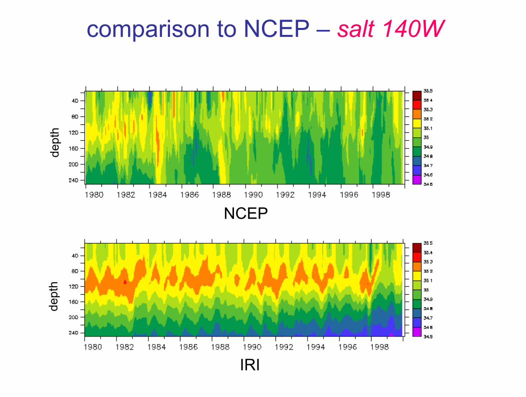
comparison to NCEP – salt 140W

NCEP

IRI

dept

hde

pth

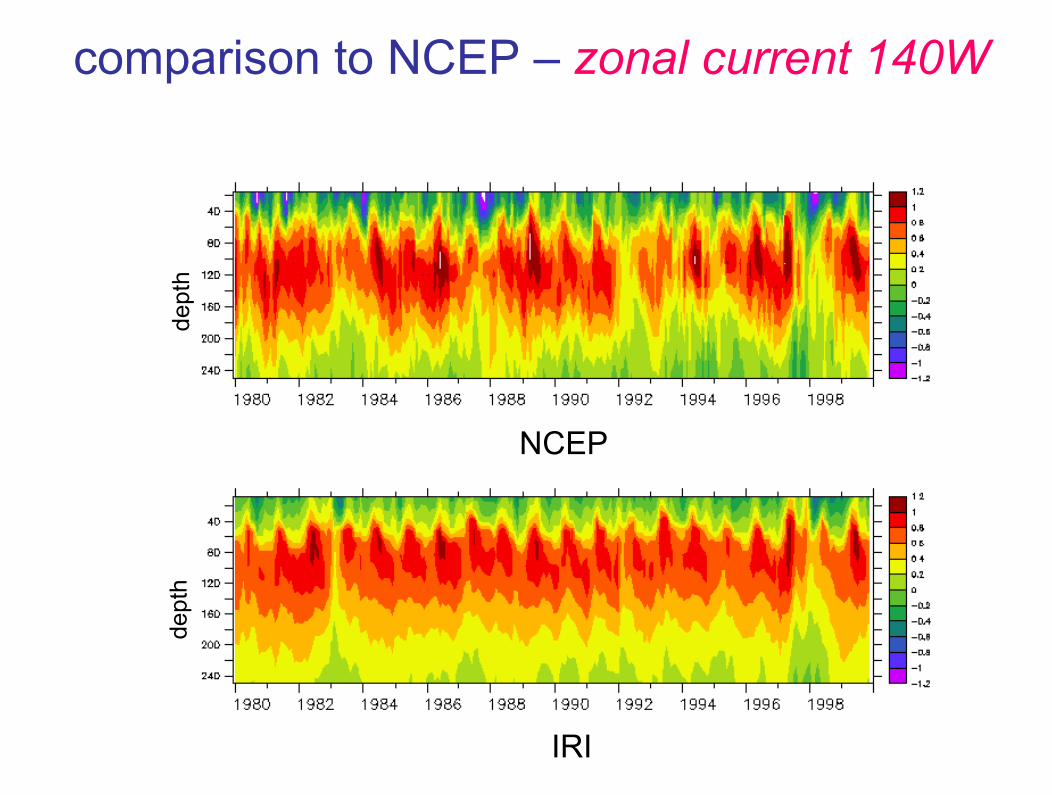
comparison to NCEP – zonal current 140W

NCEP

IRI

dept

hde

pth

Strong vs. weak assimilation

SST

Z20

_____ no assim__ __ weak assim_ _ _ strong_assim

(Analysis – observations)



Temp110W

Temp140W


Interannualvariability


Now that the system is set up, we want to experiment with:

• model resolution (higher)

• model physics

• surface forcings

• data assimilation scheme

⇒Try to find the optimum for IRI needs

But we can already take advantage of the new system and use it for various studies…

ENSO forecast experiments

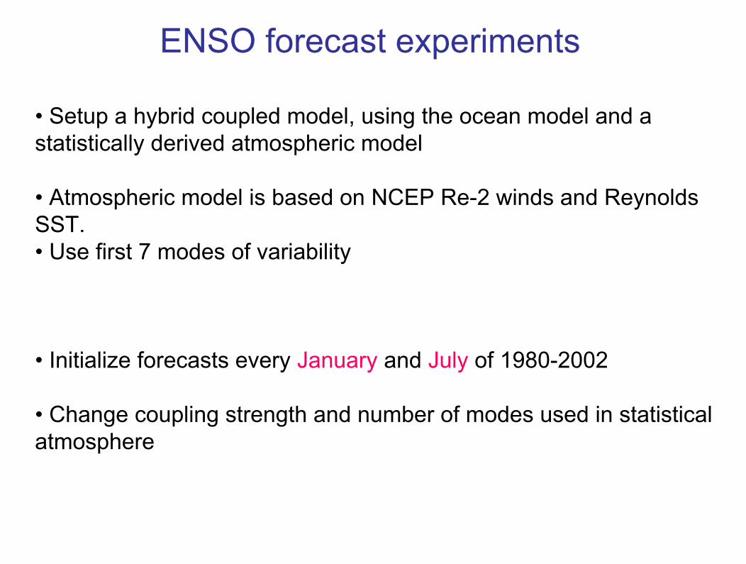
• Setup a hybrid coupled model, using the ocean model and a statistically derived atmospheric model

• Atmospheric model is based on NCEP Re-2 winds and Reynolds SST.• Use first 7 modes of variability

• Initialize forecasts every January and July of 1980-2002

• Change coupling strength and number of modes used in statistical atmosphere


no assimweak assimstrong_assim

Januaryinitialization

Julyinitialization

Coupling = 1.0


no assimweak assimstrong_assim

Januaryinitialization

Julyinitialization

Coupling = 1.5

⇒ Assessing the impact of stochastic forcing on ENSO events – the 1997 event

With Andrew Wittenberg (GFDL)

Is the atmospheric model the problem?

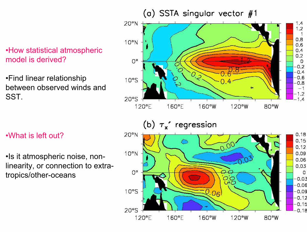
•How statistical atmospheric model is derived?

•Find linear relationship between observed winds and SST.

•What is left out?

•Is it atmospheric noise, non-linearity, or connection to extra-tropics/other-oceans

What we use -> <- what is left out

• The 1997 El-Nino event:

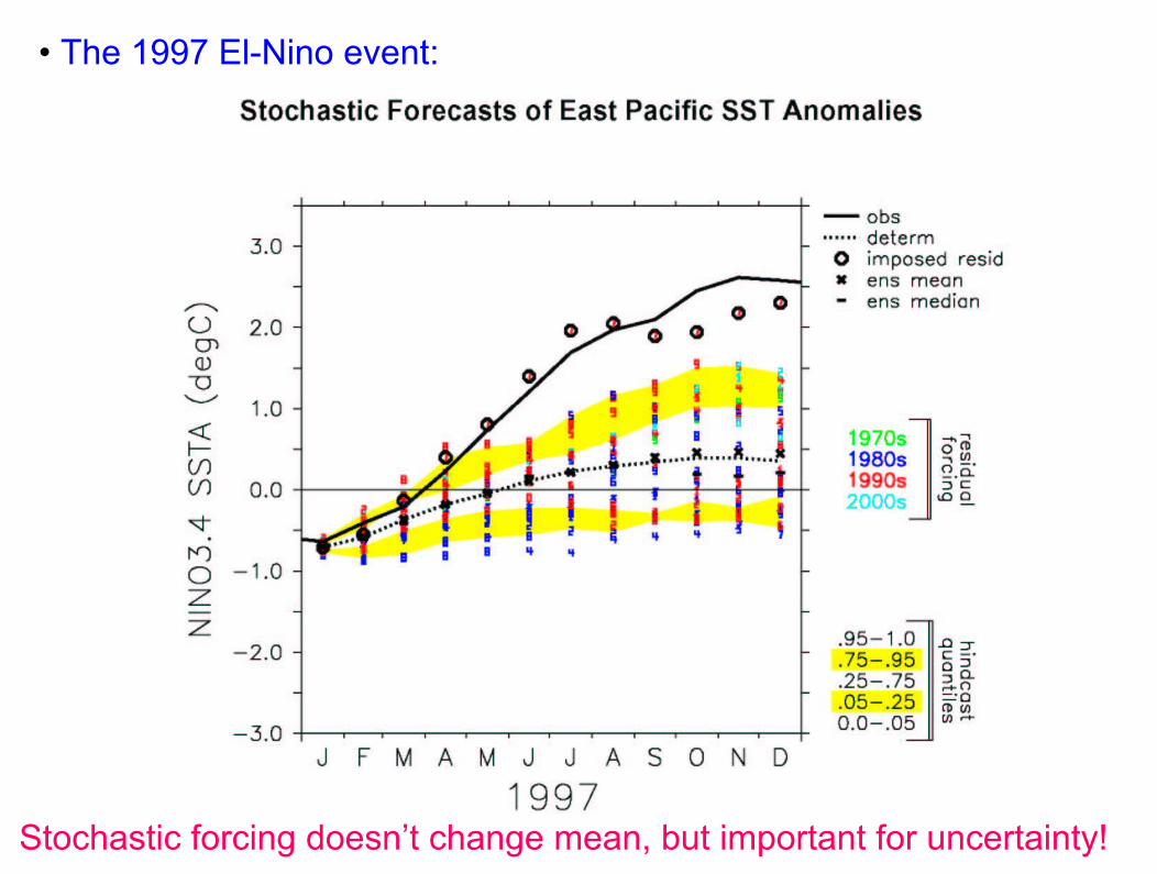
Stochastic forcing doesn’t change mean, but important for uncertainty!

• The 1997 El-Nino event:

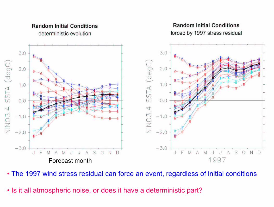
• The 1997 wind stress residual can force an event, regardless of initial conditions

• Is it all atmospheric noise, or does it have a deterministic part?

Forecast month

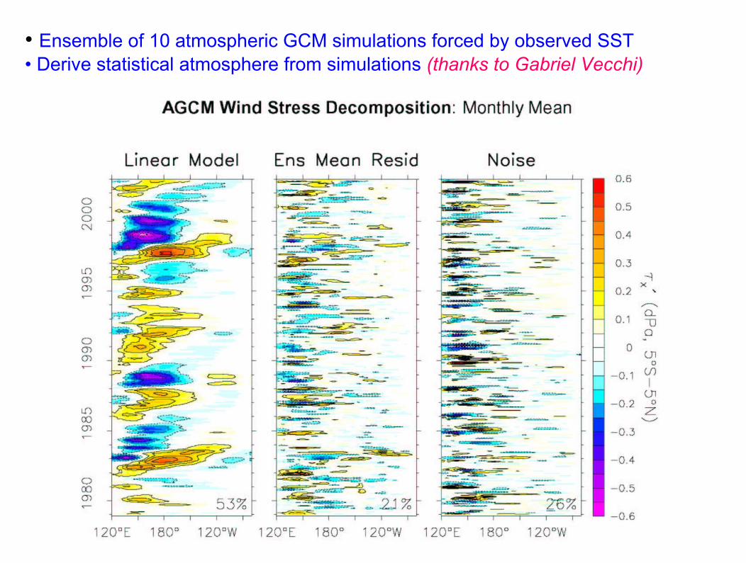
• Ensemble of 10 atmospheric GCM simulations forced by observed SST• Derive statistical atmosphere from simulations (thanks to Gabriel Vecchi)

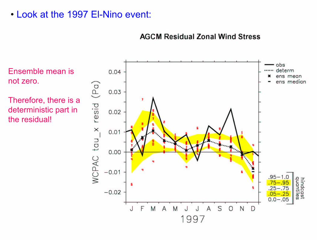
Ensemble mean is not zero.

Therefore, there is a deterministic part in the residual!

• Look at the 1997 El-Nino event:

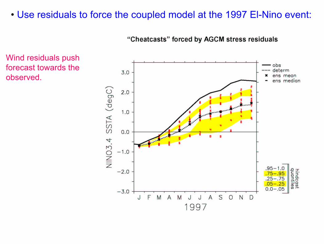
Wind residuals push forecast towards the observed.

• Use residuals to force the coupled model at the 1997 El-Nino event:

Summary of hybrid model forecasts:

• Even though Regression onto tropical Pacific SST captures most interannual variance of equatorial Pacific , the residual stress matters. It induces strong dispersion of ENSO forecasts.

• Pacific was preconditioned for warming in 1997, but unusually intense residual westerlies greatly amplified the warming.

• The residual stress is not entirely random. Even the “noise part”has structure.

• Is it non-linearity or dependence of wind on other regions SST?

The TAO east/west experiment

Thanks to Michele Rienecker (GMAO/NASA)

What can we say about the TAO array using current ENSO forecast models?

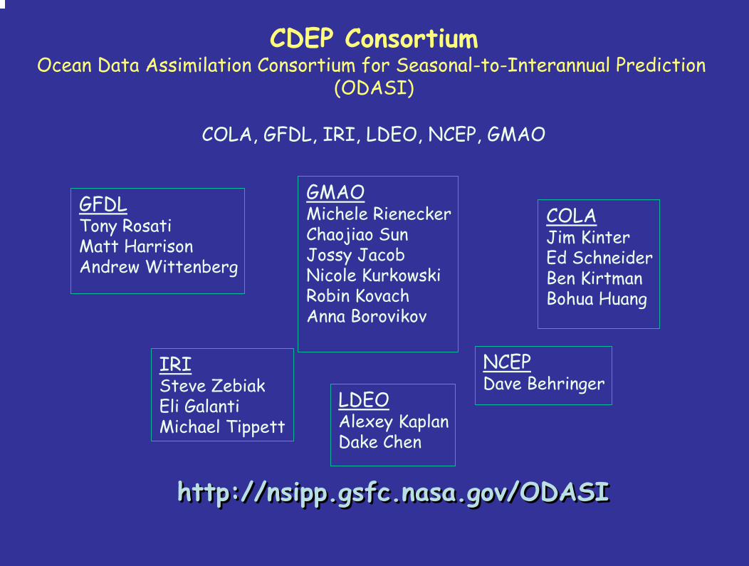
CDEP ConsortiumOcean Data Assimilation Consortium for Seasonal-to-Interannual Prediction

(ODASI)

COLA, GFDL, IRI, LDEO, NCEP, GMAO

http://nsipp.gsfc.nasa.gov/ODASIhttp://nsipp.gsfc.nasa.gov/ODASI

COLAJim KinterEd SchneiderBen KirtmanBohua Huang

GMAOMichele RieneckerChaojiao SunJossy JacobNicole KurkowskiRobin KovachAnna Borovikov

GFDLTony RosatiMatt HarrisonAndrew Wittenberg

IRISteve ZebiakEli GalantiMichael Tippett

LDEOAlexey KaplanDake Chen

NCEPDave Behringer

The Experiments:

** initial conditions for 1 January and 1 July, 1993 to 2002

** Forecast duration: 12 months

** The observations:historical XBTs, TAO array, and Argo profiles

** Surface forcing: NCEP reanalysis, and restoration to observed SST and SSS

Initial conditions for forecast experiments prepared using1. All in situ temperature profiles, including the full TAO array2. Western Pacific (west of 170°W) TAO moorings3. Eastern Pacific TAO moorings

Hypothesis: the Eastern Pacific data important for shorter lead forecasts and the Western Pacific data important for longer lead forecasts.

CGCM1

hybrid1 hybrid2a hybrid2b Intermed1

CGCM2a CGCM2b

January StartsJanuary Starts

All TAO mooringsWest TAO mooringsEast TAO mooringsObs (Reynolds)

Niño-3 SST anomaliesNiño-3 SST anomalies

hybrid2b

Intermed1

CGCM2a CGCM2b

July StartsJuly Starts

hybrid2a Intermedhybrid1


Niño-3 SST anomaliesNiño-3 SST anomalies

CGCM Forecast skill - January starts - multimodel ensemble


•multimodel ensemble skill is increased vs. individual skill•West TAO experiment has less skill, but proved to be important in central Pacific

Niño3Niño3

Niño4Niño4

January startsJanuary starts July startsJuly starts

•Tendency for “all” ensemble to have tighter spread than the “east” or “west” ensembles

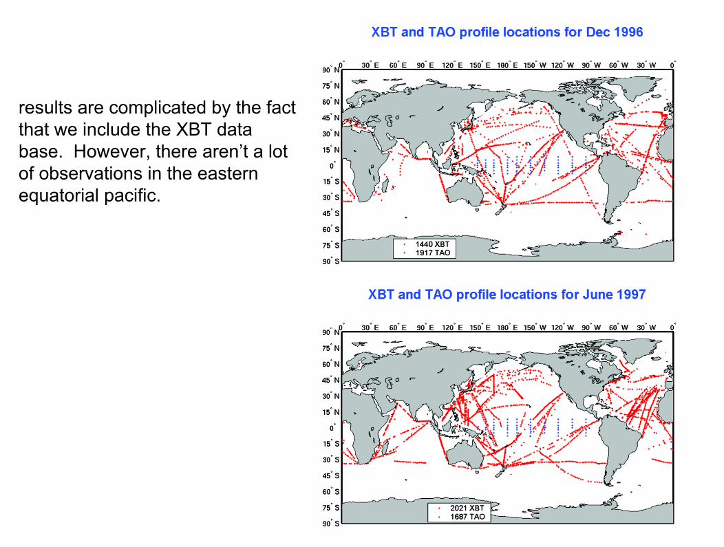
results are complicated by the fact that we include the XBT data base. However, there aren’t a lot of observations in the eastern equatorial pacific.

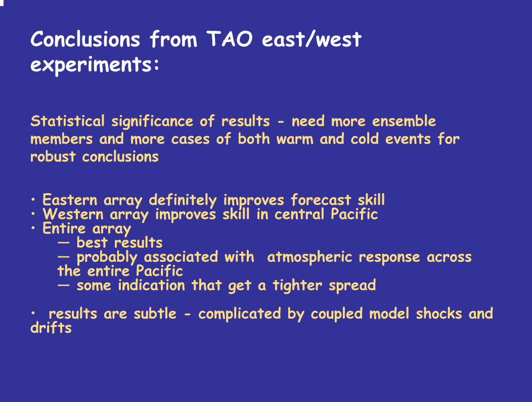
Conclusions from TAO east/west experiments:

Statistical significance of results - need more ensemble members and more cases of both warm and cold events for robust conclusions

• Eastern array definitely improves forecast skill• Western array improves skill in central Pacific• Entire array

— best results— probably associated with atmospheric response across the entire Pacific— some indication that get a tighter spread

• results are subtle - complicated by coupled model shocks and drifts

Predictability dependence on observing system lifespan in a simple ENSO model

with Mike Tippett (IRI)

How long should we observe in order to see improvement in forecast skill?

• Derive ‘reality’ from integration of simple ENSO model

• Predict ‘reality’ when initial state is not perfectly known (lack of observations)

• Improve observation in central equatorial Pacific

• Compare skill of improved system to standard one, for different lifetimes of new observing system.

The strategy

The ENSO toy model

(used in Galanti and Tziperman 2000)

Delayed equation for the east equatorial SST, function of:

•Kelvin waves – equatorial central and west Pacific subsurface

•Rossby waves – equatorial west Pacific and off-equatorial Pacific subsurface

•SST – east equatorial subsurface

•Stochastic noise

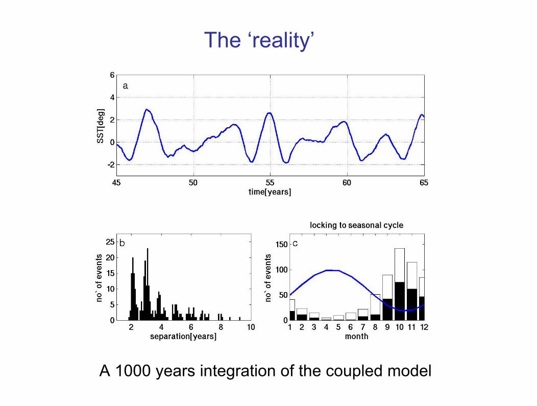
The ‘reality’

A 1000 years integration of the coupled model

The forecasts

•Add uncertainty to initial conditions using normally distributed errors (blue curve)•Reduce uncertainty in Kelvin waves initial conditions (green curve)

What happens to improvement in skill when new observing system is limited in time?

Forecast skill

Lead time (months)

corr

elat

ion

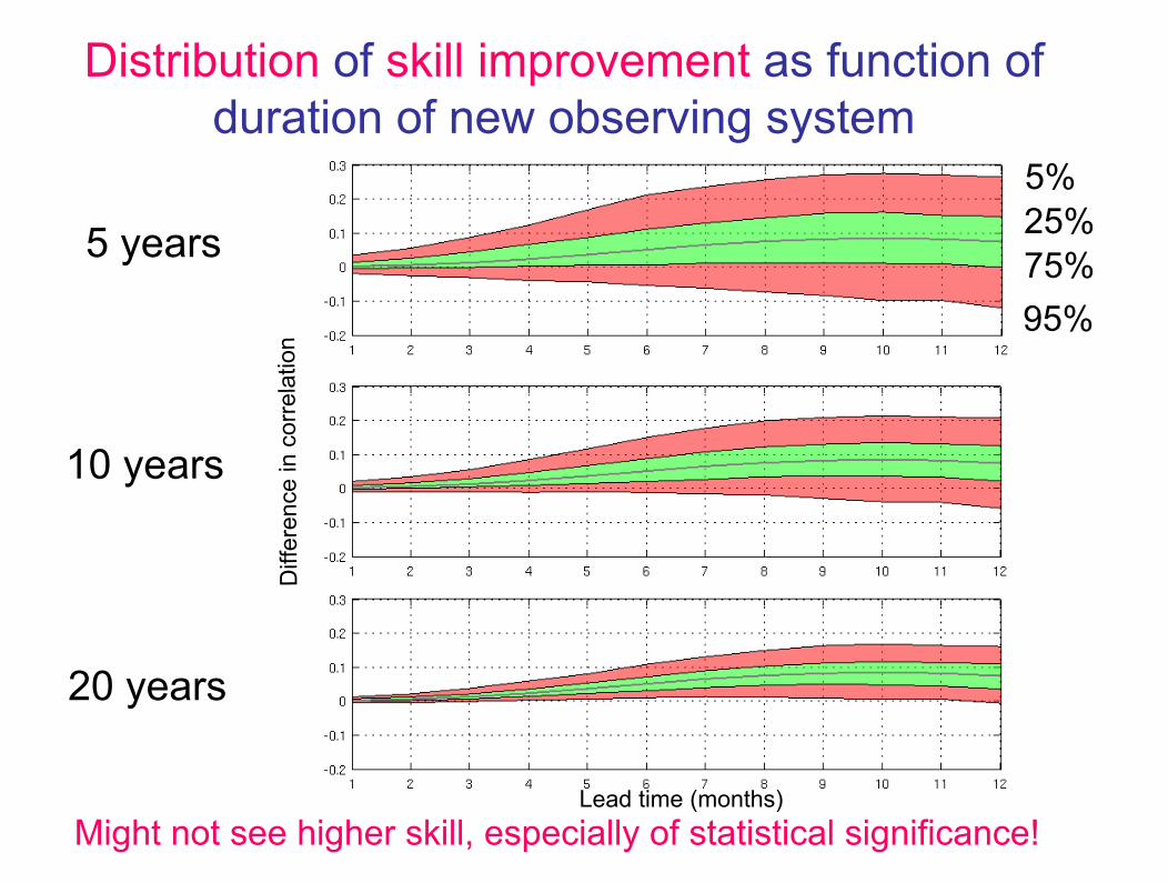
Distribution of skill improvement as function of duration of new observing system

5 years

10 years

20 years

5%25%75%95%

Might not see higher skill, especially of statistical significance! Lead time (months)

Diff

eren

ce in

cor

rela

tion

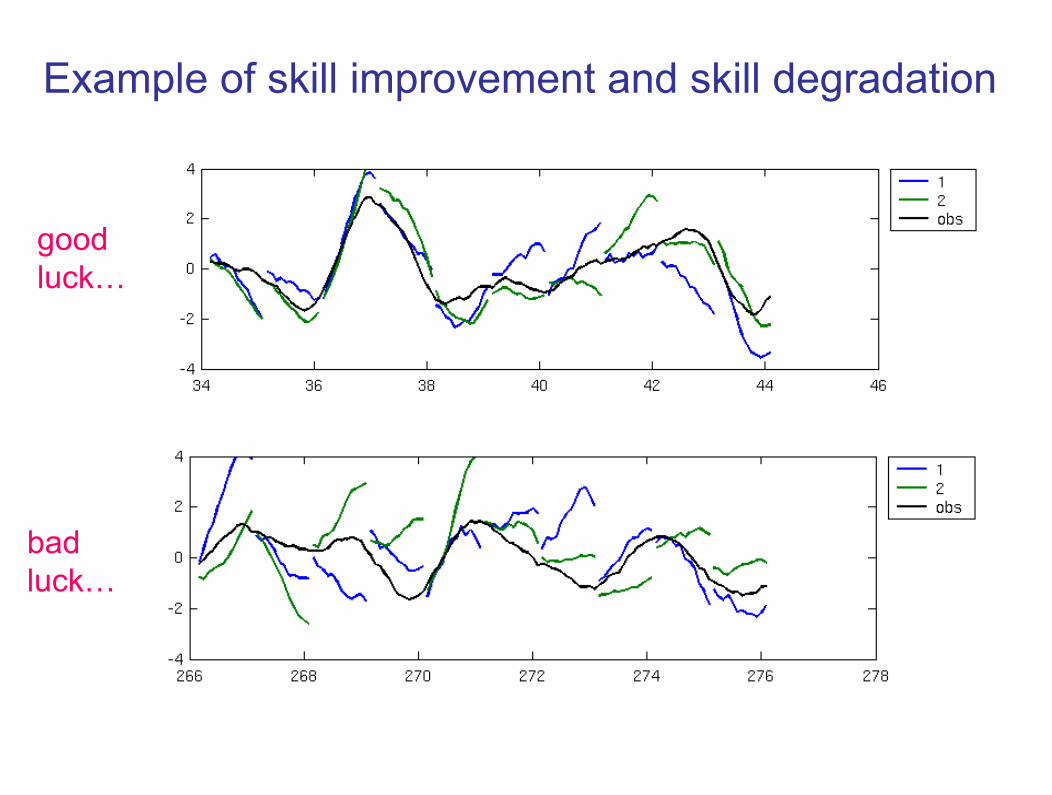
Example of skill improvement and skill degradation

goodluck…

badluck…

Seasonality in skill improvement

Forecast skillFrom the 1000yr

standard improved difference

5 years 10 years 20 years

Probability of improving skill

TAO east/west

Take home message…

• Given that a new observing system exists for only a short period, even within a framework of a simplified reality and model, improvement in forecast skill is not guaranteed to be seen.

•Including seasonality in analysis makes judgment of skill improvement even harder.

Summary of talk:

• The new IRI ocean data assimilation system

• ENSO forecast experiments and the role of stochastic forcing

• The TAO array east/west experiment

• Measuring impact of observing system’s lifetime in a simple model

On data assimilation and ENSO dynamical prediction

Documents

Transcript of On data assimilation and ENSO dynamical prediction