ON CHI-SQUARE DIFFERENCE AND z TESTS IN MEAN …kyuan/courses/sem/readpapers/... · ON CHI-SQUARE...

10.1177/0013164404264853EDUCATIONAL AND PSYCHOLOGICAL MEASUREMENT

YUAN AND BENTLER

ON CHI-SQUARE DIFFERENCE AND z TESTS IN MEANAND COVARIANCE STRUCTURE ANALYSIS WHEN

THE BASE MODEL IS MISSPECIFIED

KE-HAI YUANUniversity of Notre Dame

PETER M. BENTLERUniversity of California, Los Angeles

In mean and covariance structure analysis, the chi-square difference test is often appliedto evaluate the number of factors, cross-group constraints, and other nested model com-parisons. Let model Ma be the base model within which model Mb is nested. In practice,this test is commonly used to justify Mb even when Ma is misspecified. The authors studythe behavior of the chi-square difference test in such a circumstance. Monte Carlo resultsindicate that a nonsignificant chi-square difference cannot be used to justify the con-straints in Mb. They also show that when the base model is misspecified, the z test for thestatistical significance of a parameter estimate can also be misleading. For specific mod-els, the analysis further shows that the intercept and slope parameters in growth curvemodels can be estimated consistently even when the covariance structure is misspecified,but only in linear growth models. Similarly, with misspecified covariance structures, themean parameters in multiple group models can be estimated consistently under nullconditions.

Keywords: chi-square difference; nested models; model misspecification; parameterbias; mean comparison; growth curves

Measurements in the social and behavioral sciences are typically subjectto errors. By separating measurement errors from latent constructs, structural

This research was supported by Grant DA01070 from the National Institute on Drug Abuseand by a Faculty Research Grant from the Graduate School at the University of Notre Dame. Cor-respondence concerning this article should be addressed to Ke-Hai Yuan, Department of Psy-chology, University of Notre Dame, Notre Dame, IN 46556; e-mail: [email protected].

Educational and Psychological Measurement, Vol. 64 No. 5, October 2004 737-757DOI: 10.1177/0013164404264853© 2004 Sage Publications

737

equation modeling (SEM) provides means of modeling the latent variablesdirectly (e.g., Bollen, 2002; MacCallum & Austin, 2000). Compared to mod-els that do not take measurement errors into account, SEM can provide moreaccurate conclusions regarding the relationship between interesting attrib-utes. To achieve such an objective, the methodology of SEM has to be appro-priately used. In practice, researchers often elaborate on the substantive sideof a structural model even when it barely fits the data. We will show that sucha practice most likely leads to biased or misleading conclusions. Specifically,we will discuss the misuse of the chi-square difference test and the z test. Forthe discussion of the misuse of the chi-square difference test, we will focus onusing this test in deciding the number of factors and for adding cross-groupconstraints. For the discussion of the misuse of the z test, we will focus on itsuse in evaluating the statistical significance of mean parameter estimates inthe growth curve models and latent mean comparisons.

There are many indices for evaluating the adequacy of a model. Amongthese, only a chi-square statistic judges the model using probability as char-acterized by Type I and Type II errors. Although the chi-square test is limiteddue to its reliance on sample sizes, it is still commonly reported in applica-tions. In practice, many reported chi-square statistics are significant evenwhen sample sizes are not large, and in the context of nested models, the chi-square difference test is often not significant; this is used to justify modelmodifications or constraints across groups (e.g., Larose, Guay, & Boivin,2002). The practice for relying on difference tests has a long history inpsychometrics. For example, in the context of exploratory studies, Jöreskog(1978) stated,

If the drop in χ 2 is large compared to the difference in degrees of freedom, thisis an indication that the change made in the model is a real improvement. If, onthe other hand, the drop in χ 2 is close to the difference in number of degrees offreedom, this is an indication that the improvement in fit is obtained by “capi-talization on chance” and the added parameters may not have any real signifi-cance or meaning. (p. 448)

This statement may give encouragement for using the chi-square differencetest to guide model modifications or adding constraints even when the lessconstrained model is highly significant. We will show that the difference testcannot be used reliably in this manner.

We will mainly study the misuse of statistical significance tests. In thecontext of multiple groups, even when a model may barely fit an individualsample, further constraints may be added across the groups. Let Ta be the sta-tistic corresponding to the models without the constraints and Tb be the statis-tic corresponding to the models with constraints. Even when both Ta and Tb

are statistically significant, implying rejection of both models, the difference∆T = Tb – Ta can still be nonsignificant. This is often used to justify the cross-

738 EDUCATIONAL AND PSYCHOLOGICAL MEASUREMENT

group constraints in practice. See Drasgow and Kanfer (1985), Brouwers andTomic (2001), and Vispoel, Boo, and Bleiler (2001) for such applications.Similarly, a model with two factors may correspond to a significant statisticTa whereas the substantive theory may support only a one-factor model. Theone-factor model may have a significant statistic Tb. In such a context, manyresearchers regard the one-factor model as “attainable” if ∆T = Tb – Ta is notstatistically significant at the .05 level. In the context of latent growth curvesand latent mean comparisons, there are mean structures in addition tocovariance structures. These models are nested within the covariance struc-ture models with saturated means. The statistic Ta corresponding to only thecovariance structure may be already highly statistically significant. Adding amean structure generally makes the overall model even more statistically sig-nificant, that is, less fitting. Nonetheless, researchers still elaborate on thesignificance of the intercept or slope estimates or significant meandifferences as evaluated by z tests.

Let the model Ma be the base model within which model Mb is nested.When Ma is an adequate model as reflected by a nonsignificant Ta and sup-ported by other model fit indices, one may want to test the further restrictedmodel Mb. If ∆T = Tb – Ta is not statistically significant, Mb is generally pre-ferred because it is more parsimonious. When Ma is not adequate as indicatedby a significant Ta, can we still justify Mb by a nonsignificant ∆T? Althoughthere exist statistical theories (Steiger, Shapiro, & Browne, 1985) in this con-text, and wide applications (e.g., Brouwers & Tomic, 2001; Drasgow &Kanfer, 1985; Vispoel et al., 2001) justify Mb using nonsignificant ∆Ts, in ourview, the effect of such a practice on the substantive aspect of SEM is notclear. A related question is when the overall model is misspecified, can a testbe used to indicate the statistical significance of a parameter estimate? Exam-ples in this direction include whether the intercept and slope parameters in alatent growth curve model are zeros, whether the means are different in latentmean comparisons, and whether a parameter should be freed or fixed as inmodel modifications. The interest here is to study the effect of misspecifiedmodels on ∆T and the z tests. By simulation, the second section studies thebehavior of ∆T when Ma is misspecified. The third section explores the rea-son why ∆T does not perform properly when Ma is misspecified. Detailedresults show that a misspecified model leads to biased parameters, whichexplains why model inferences based on ∆T and parameter inference basedon the z test actually can be quite misleading.

Chi-Square Difference TestWhen the Base Model Is Misspecified

Jöreskog (1971) and Lee and Leung (1982) recommended using the chi-square difference test for cross-group constraints in analyzing multiple sam-

YUAN AND BENTLER 739

ples. Under some standard regularity conditions, Steiger et al. (1985) provedthat the chi-square difference statistic asymptotically follows a noncentralchi-square distribution (see also Satorra & Saris, 1985). Chou and Bentler(1990) studied the chi-square difference test when Ma is correctly specifiedand found that it performs the best compared to the Lagrange multiplier testand the Wald test in identifying omitted parameters. The chi-square differ-ence test has been widely used in SEM, essentially in every application ofSEM with multiple groups. However, how to appropriately apply the chi-square difference test in practice is not clear at all. Paradoxes readily occur,for example, a nonsignificant Ta and a nonsignificant ∆T = Tb – Ta cannotguarantee a statistically nonsignificant Tb. Although Ta = 3.84 ~ χ1

2 is statisti-cally nonsignificant at the .05 level and ∆Tb = 3.84 ~ χ1

2 is statisticallynonsignificant at the .05 level, Tb = 7.68 ~ χ 2

2 is statistically significant at .05level. Another paradox occurs when sequential application of nonsignificant∆T may lead to a highly significant final model. The general point is thatwhen ∆T is not statistically significant, one may derive the conclusion that Mb

is less misspecified than Ma. However, we will show that this is not necessar-ily the case. In this section, we will show the effect of a misspecified basemodel Ma on the significance of ∆T through three simulation studies.Because the normal theory-based likelihood ratio statistic TML is commonlyused in practice, we study only the performance of ∆T based on this statisticfor simulated normal data. When data are not normal or when another statis-tic is used in practice, one cannot expect ∆T to perform better.

Type II Error of ∆T in Deciding the Number of Factors

We first study using ∆T to judge the number of factors in a confirmatoryfactor model. Using ∆T to decide the number of factors in the exploratory fac-tor model was recommended by Lawley and Maxwell (1971). It is also com-monly applied when confirmatory factor analysis is used for scaledevelopment.

Let us consider a confirmatory factor model with five manifest variablesand two latent factors. The population is generated by

x = �0 + f + e

with

E(x) = �0, Cov(x)= �0 = �0�0 ′�0 + �o, (1)

where

� �07000

7900

0926

0774

0725

1 0818

818=

′

=. .. . . , .

..

0 1 0. ,


ψ150 = ψ510 = 0.285, and the diagonal elements of 0 are adjusted so that 0 isa correlation matrix. Note that the subscript 0 is used to denote the populationvalue of a parameter. The corresponding model parameter without the sub-script 0 is subject to estimation before its value can be obtained. Except forψ150, the population parameter values for the model defined in Equation 1 areobtained from fitting the two-factor model to the open-closed book data set inTable 1.2.1 of Mardia, Kent, and Bibby (1979). The purposes of choosingthis set of population values are (a) they are represented by real data and thusrealistic, (b) φ120 = 0.818 is large enough so that ∆T will not be able to judgethe correct number of factors when Ma is misspecified.

Let the covariance structure model be

M(�) = ��′ + � ,

where

� �=

′

=

λ λλ λ λ φ

φ11 21

32 42 52 21

120 0

0 0 0 1 01 0

, ..

and � is a diagonal matrix. Because we ignore the covariance ψ15, the abovetwo-factor model is no longer correct for the population covariance matrix inEquation 1. Of course, the one-factor model excluding ψ15 is not correcteither. In such a circumstance, however, a researcher may be tempted in prac-tice to justify the one-factor model by a nonsignificant ∆T. We next evaluatethe effect of ignoring ψ15 on ∆T for such a purpose.

Without a mean structure, there is only one degree of freedom differencebetween Ma (the one-factor model) and Mb (the two-factor model). We refer∆T to the 95th percentile of χ1

2 for statistical significance. With 500 replica-tions, Table 1 contains the number of replications with nonsignificant ∆T. Forcomparison purposes, we also include the performance of ∆T when ψ15 isexplicitly included in both Ma and Mb. When ψ15 is excluded, although theone-factor model is inadequate due to a misspecification, ∆T cannot rejectthe one-factor model more than 50% at sample size n = 100. With correctmodel specification in Ma, ∆T has a much greater power to reject the wrongmodel Mb.

Type II Error of ∆T in TestingInvariance in Factor Pattern Coefficients

With a misspecified base model Ma, the statistic ∆T not only loses itspower with smaller sample sizes but also may have a weak power even withvery large sample sizes. We will illustrate this through a two-groupcomparison.


Consider two groups, each with four manifest variables that are generatedby a one-factor model. The population covariance matrix �10 of the firstgroup is generated by

x1 = �10��10 f1 + e1,

where

�10 = (1, 0.80, 0.50, 0.40)′, Var(f1) = φ0(1) = 1.0, Cov(e1) = �10 = (ψ ij0

1( )),

with ψ ψ ψ ψ ψ1101

2201

3301

4401

14010 124 109( ) ( ) ( ) ( ). , . , . ,= = = = ( ) .1 32= , and ψ 2401 25( ) .= .

The population covariance matrix �20 of the second group is generated by

x2 = �20 + �20 f2 + e2,

where

�20 = (1, .80, .70, .80)′, Var(f2) = φ0(2) = 1.0, Cov(e2) = �20 = (ψ ij0

2( )),

with ψ ψ ψ ψ1102

2202

3302

4402 10( ) ( ) ( ) ( ) . ,= = = = and ψ 340

2 559( ) .= − . It is obvious thatthe two groups do not have invariant factor pattern coefficients. In model Ma,the one-factor model M(�) = �φ�′ + �, where � is a diagonal matrix, is fit-ted to a normal sample from each of the populations corresponding to �10 and�20 and the statistic Ta is the sum of the two ΤMLs. The first factor pattern coef-ficient was set at 1.0 for identification purposes. In model Mb, the three-factorpattern coefficients as well as the factor variances were set equal across thetwo groups, which results in the statistic Tb. Referring ∆T = Tb – Ta to the 95thpercentile of χ1

2 , the number of nonsignificant replications are given in themiddle column of Table 2. For the purpose of comparison, a parallel study inwhich the three error covariances are included in � in both Ma and Mb wasalso performed, and the corresponding results are in the last column of Table 2.


Table 1Number of Nonsignificant ∆T = Tb – Ta (Type II Error) Out of 500 Replications: One-FactorModel (Ma) Versus Two-Factor Model (Mb)

Sample Size Misspecified Ma and Mb Correct Ma and Misspecified Mb

50 363 176100 276 48200 148 1300 60 0400 34 0500 8 0

When ignoring the error covariances, only 494 replications out of the 500converged when n1 = n2 = 100, and 497 replications converged when n1 = n2 =200. When error covariances were accounted for, 496 replications convergedwhen n1 = n2 = 100. The number of nonsignificant replications is based on theconverged replications only. When the base model is misspecified, althoughthe power for ∆T to reject the incorrect constraints increases as sample sizesincrease, the speed is extremely slow. Even when n1 = n2 = 1,000, more than60% of the replications could not reject the incorrect constraints. When Ma iscorrectly specified, the statistic ∆T has a power greater than 0.95 in rejectingthe incorrect constraints at sample size n1 = n2 = 500.

Type I Error of ∆T in Testing Invariance in Factor Pattern Coefficients

A misspecified Ma not only leads to attenuated power for the chi-squaredifference test, it can also lead to inflated Type I errors, as illustrated in thefollowing two-group comparison.

Again, consider two groups, each with four manifest variables that aregenerated by a one-factor model. The first group, �10 = Cov(x1), is gener-ated by

x1 = �10 + �10 f1 + e1,

where

�10 = (1, .80, .70, .50)′, Var(f1) = φ0(1) = 1.0, Cov(e1) = �10 = (ψ ij0

1( ))

with ψ ψ ψ ψ ψ1101

2201

3301

4401

140110 70( ) ( ) ( ) ( ) ( ). , .= = = = = and ψ 240

1 30( ) .= . The secondgroup, �20 = Cov(x2), is generated by


Table 2Number of Nonsignificant ∆T = Tb – Ta (Type II Error) Out of 500 Replications:Incorrect Equality Constraints Across Two-Group Factor Pattern Coefficients

Sample Size (n1 = n2) Misspecified Ma and Mb Correct Ma and Misspecified Mb

100 447/494a 342/496200 444/497 239300 417 131400 402 66500 387 23

1,000 329 13,000 66 0

a. Converged solutions out of 500 replications.

x2 = �20 + �20 f2 + e2,

where

�20 = (1, .80, .70, .50)′, Var(f2) = φ02( ) = 1.0, Cov(e2) = �20 = (ψ ij0

2( )),

with ψ ψ ψ ψ1102

2202

3302

4402 10( ) ( ) ( ) ( ) . ,= = = = and ψ 340

2 25( ) .= − . Now, the two groupshave invariant factor pattern coefficients and factor variances. We want toknow whether ∆T can endorse the invariance when Ma is misspecified. Letthe three error covariances be ignored in Ma when fitting the one-factormodel to both samples and Mb be the model in which the factor pattern coeffi-cients and factor variances are constrained equal. Instead of reporting thenonsignificant replications of ∆T, we report the significant ones in Table 3.When Ma is misspecified, ∆T is not able to justify the cross-group constraints.As indicated in Table 3, even when n1 = n2 = 100, more than 70% of the equalfactor pattern coefficients and factor variances are rejected. When the errorcovariances were accounted for in Ma and Mb, Type I errors are around thenominal level of 5% for all the sample sizes in Table 3.

In summary, when the base model Ma is misspecified, the chi-square dif-ference test cannot control either the Type I errors or the Type II errors forrealistic sample sizes. Conclusions based on ∆T are misleading. For the simu-lation results in Tables 1 to 3, we did not distinguish the significant Tas fromthose that are not significant. Some of the nonsignificant ∆Ts in Tables 1 and2 have nonsignificant Tas, and some of the significant ∆Ts in Table 3 also cor-respond to nonsignificant Tas. As was discussed at the beginning of this sec-tion, even when both Ta and ∆T are not significant at the .05 level, we areunable to control the errors of inference regarding model Mb. When con-straints across groups hold partially, Kaplan (1989) studied the performanceof TML, which is essentially the Tb here. The results in Tables 1 to 3 are not inconflict with Kaplan’s results, which indicate that Tb has a nice power indetecting misspecifications. Actually, both Ta and Tb can also be regarded aschi-square difference tests due to Ma and Mb being nested within the saturatedmodel Ms. Because Ms is always correctly specified, Ta and Tb do not possessthe problems discussed above.

Because ∆T, the Lagrange multiplier, and the Wald tests are asymptoti-cally equivalent (Buse, 1982; Lee, 1985; Satorra, 1989), the results in Tables1 to 3 may also imply that the two other tests cannot perform well in similarcircumstances. All of these tests are used in model modification, and ourresults may explain some of the poor performance of empirically basedmodel modification methods (e.g., MacCallum, 1986).

Steiger et al. (1985) showed that chi-square differences in sequential testsare asymptotically independent, and each difference follows a noncentralchi-square even when Ma is misspecified. The results in this section imply


that (a) when the base model Ma is wrong and the constraints that differentiateMa and Mb are substantially incorrect, the noncentrality parameter of the chi-square difference can be tiny so that ∆T loses its power and (b) when thebase model Ma is wrong and the constraints that differentiate Ma and Mb arecorrect, the noncentrality parameter of the chi-square difference can besubstantial so that ∆T always rejects the correct hypothesis. The next sec-tion explains why the noncentrality parameter is tiny or substantial due tomisspecifications.

The Effect of a Misspecified Model on Parameters

In this section, we explain why the chi-square difference test is misleadingwhen the base model is misspecified. Specifically, when a model ismisspecified, parameter estimates converge to different values from those ofa correctly specified model. Thus, equal parameters in a correctly specifiedmodel become unequal in a misspecified model. Consequently, ∆T for test-ing constraints will be misleading. In the context of mean structures, ratherthan using a chi-square statistic to evaluate the overall model, researchersoften use z tests to evaluate the statistical significance of mean parameter esti-mates (see Hong, Malik, & Lee, 2003; Whiteside-Mansell & Corwyn, 2003).We will also show the effect of a misspecified model in evaluating the meanparameters. We use results in Yuan and Bentler (2004) for this purpose.

Let x and S be the sample mean vector and sample covariance matrix froma p-variate normal distribution Np(�0, �0). Let *() and M*() be thecorrect mean and covariance structure; thus, there exists a vector 0 suchthat �0 = *(0) and �0 = M*(0). Let the misspecified model be (�) andM(�). We assume that the misspecification is due to model (�) and M(�)missing parameters � of = (�′, �′)′. In the context of mean and covariancestructure analysis, one obtains the normal theory-based maximum likelihoodestimate (MLE) ��of�0 by minimizing (see, e.g., Browne & Arminger, 1995)

FML(�, x, S) = [x – (�)]′M–1(�)[x – (�)] + tr[SM–1(�)] – log|SM–1(�)| – p.


Table 3Number of Significant ∆T = Tb – Ta (Type I Error) Out of 500 Replications: Correct EqualityConstraints Across Two-Group Factor Pattern Coefficients

Sample Size (n1 = n2) Misspecified Ma and Mb Correct Ma and Mb

100 362/497a 25200 481 28300 498 23400 500 25

a. Converged solutions out of 500 replications.

Under some standard regularity conditions (e.g., Kano, 1986; Shapiro,1984), �� converges to �*, which minimizes FML(�, �0, �0). Note that in gen-eral,�* does not equal its counterpart�0 in � �0 0 0= ′ ′ ′( , ) , which is the popu-lation value of the correctly specified model. We will call ∆� =�* –�0 the biasin�*, which is also the asymptotic bias in ��. It is obvious that if the sample isgenerated by �0 = (�0) and �0 = M(� 0 ), then �* will have no bias. We mayregard the true population (�0, �0) as a perturbation to (�0, �0). Because ofthe perturbation, �* ≠ �0, although some parameters in �* can still equal thecorresponding ones in �0 (see Yuan, Marshall, & Bentler, 2003). Yuan et al.(2003) studied the effect of the misspecified model on parameter estimates incovariance structure analysis. Extending their result to mean and covariancestructure models, Yuan and Bentler (2004) characterized� as a function of �and � in a neighborhood of (�0, �0). Denote this function as � = g(�, �),where � is the vector containing the nonduplicated elements of �. Then thereapproximately exists

∆ ∆ ∆� � � � � � �≈ � ( , ) � ( , )g g10 0

20 0+ , (2)

where �g1 is the partial derivative of g with respect to � and �g 2 is the partial de-rivative of g with respect to �; ∆�0 = �0 – �0 and ∆� = �0 – �0. Explicit ex-pressions of �g1 and �g 2 are given in Yuan and Bentler (2004). Equation 2 im-plies that the bias in�* caused by ∆� and ∆� are approximately additive. Letq be the number of free parameters in �, and then �g1 (�0, �0) is a q × p matrixand �g 2 (�0, �0) is a q × p* matrix, where p* = p(p + 1)/2. For the lth parameterθl, we can rewrite Equation 2 as

∆ ∆ ∆θ µ σl ≈ += ==∑ ∑∑c clii

p

i lijj

p

i

p

ij1 11

. (3)

When the parameter is clear, we will omit the subscript in reporting the coef-ficients in examples.

Now we can use the result in Equation 2 or Equation 3 to explain the mis-leading behavior of ∆T when Ma is misspecified. Because of themisspecification,�* may not equal�. Most nested models can be formulatedby imposing constraints h(�) = 0. When h(�0) = 0, h(�*) may not equal zero.With a misspecified Ma, it is the constraints h(�*) = 0 that are being tested by∆T. Because h(�*) ≠ 0, Tb will be significantly greater than Ta, and thus ∆Ttends to be statistically significant as reflected in Table 3. Similarly, whenh(�0) does not equal zero, h(�*) may approximately equal zero. Conse-quently, the power for ∆T to reject h(�*) = 0 is low, as reflected in Tables 1and 2. However, researchers in practice treat h(�0) = 0 as plausible.


In general, it is difficult to control the two types of errors by ∆T when Ma ismisspecified. If treating ∆T as if Ma were correctly specified when it is actu-ally not, the conclusion regarding h(�0) = 0 will be misleading. For example,the ∆T that produced the results in Table 1 tests whether φ120 = 1. Whenignoring ψ15 in M(�), using Equation 3 and the population parameter valuesin Table 1, we have ∆φ12 ≈ 0.166 ∆σ15 = 0.166 × 0.285 = 0.047. This leads toφ12

* ≈ 0.865, which is closer to 1.0 than φ120 = 0.818. Actually, any positiveperturbation on σij, i = 1,2; j = 3,4,5 will cause a positive bias in φ12

* , as illus-trated in the following example.

Example 1

Let �0 be the population parameter values of the model in Equation 1excluding ψ150; evaluating Equation 3 at �0, we obtain the coefficients cij forthe approximate bias cij∆σij of φ12

* in Table 4. For purposes of comparison, theexact biases when ∆σij = 0.05, 0.10, and 0.20 were also computed by mini-mizing FML(�, �0, �0) directly. The approximate biases cij∆σij are very closeto the exact ones when ∆σij = 0.05. The accuracy of the approximationdecreases as the amount of perturbation ∆σij increases. This is because Equa-tion 2 is based on a local linearization. The smallest cij is with σ45, implyingthat the function φ12 = φ12(�) is quite flat in the direction of σ45. The directionobtained at this point is usually not stable. Actually, the c45∆σ45 predicts asmall positive bias in φ12

* when ∆σ45 = 0.10 or 0.20, but the actual biases arenegative. Except for this element, the predicted biases and the actual biasesagree reasonably well for perturbations on all the other covariances σij.Notice that positive perturbations on the covariances between indicators fordifferent factors (σij, i = 1,2; j = 3,4,5) lead to an inflated φ12

* . Perturbations inthe opposite direction will lead to an attenuated φ12

* . So the estimate �φ12 andany testing for φ120 = 0 or 1 based on �φ12 are not trustworthy when model Ma ismisspecified, especially when φ120 is near 0 or 1.0.

Similarly, due to the changes in parameters, the chi-square difference testfor the equivalent constraints across groups is misleading when either of themodels does not fit the data within a group. Instead of providing more exam-ples about the bias on factor pattern coefficients when σij are perturbed, weillustrate the effect of a misspecified model on the mean parameters in simul-taneously modeling mean and covariance structures.

Let y = (y1, y2, …, yp)′ be repeated measures at p time points. Then a latentgrowth curve model can be expressed as (Curran, 2000; Duncan, Duncan,Strycker, Li, & Alpert, 1999; McArdle & Epstein, 1987; Meredith & Tisak,1990)

y = �f + e, (4)


where

� =

′

−1 00

1 01 0

1 0 1 01 2

. ..

. . ,λ λ…… p

f = (f1, f2)′, with f1 being the latent intercept and f2 being the latent slope, �f =E(f) = (α, β)′,

� = =

Cov( )f

φφ

φφ

11

21

12

22

and Cov(e) = � = diag(ψ11, ψ22, …, ψpp). This setup leads to the followingmean and covariance structures:

(�) = ��f, M(�) = ��′ + �.

In fitting such a model in practice, researchers often need to elaborate on thesignificance of the parameter estimates �α and �β, although the overall modelfit is typically significant as judged by a chi-square statistic. If themisspecification affects the mean structure to such a degree that thesignificances of �α and �β are due to only a systematic bias, then caution isneeded to specify the model before meaningful �α and �β can be obtained. Wewill consider the models for both linear growth and nonlinear growth.


Table 4The Effect of a Perturbation ∆σij on Factor Correlation φ12

*

∆σij = 0.05 ∆σij = 0.10 ∆σij = 0.20

σij cij cij × ∆σij ∆φ12 cij × ∆σij ∆φ12 cij × ∆σij ∆φ12

σ12 –0.740 –0.037 –0.035 –0.074 –0.065 –0.148 –0.117σ13 0.464 0.023 0.023 0.046 0.044 0.093 0.068σ14 0.212 0.011 0.011 0.021 0.024 0.042 0.056σ15 0.166 0.008 0.009 0.017 0.018 0.033 0.041σ23 0.363 0.018 0.017 0.036 0.031 0.073 0.032σ24 0.221 0.011 0.012 0.022 0.025 0.044 0.058σ25 0.173 0.009 0.009 0.017 0.019 0.035 0.044σ34 –0.362 –0.018 –0.020 –0.036 –0.042 –0.072 –0.090σ35 –0.305 –0.015 –0.018 –0.030 –0.040 –0.061 –0.092σ45 0.097 0.005 0.002 0.010 –0.002 0.019 –0.046

Example 2

When letting λ1 = 2, λ2 = 3, . . . , λp – 2 = p – 1, Equation 4 describes the lineargrowth model. The unknown parameters in this model are

� = (α, β, φ11, φ21, φ22, ψ11, . . . , ψpp)′.

Detailed calculation (see Yuan & Bentter, 2004) shows that all the c1ijs andc2ijs in Equation 3 are zero. So there is no effect of misspecification in M(�)on α* and β*. This implies that we can still get consistent parameter esti-mates �αand �β when (�) is correctly specified even if M(�) is misspecified.

However, the misspecification in (�) does have an effect on α* and β* aspresented in Table 5 using p = 4, where Equation 3 was evaluated at

α0 = 1, β0 = 1, φ110 = φ220 = 1.0, φ120 = 0.5, ψ110 = … = ψpp0 = 1.0,

and the perturbation was set at ∆µi = 0.2. The positive perturbations ∆µ1 and∆µ2 cause positive biases on α* but negative biases on β*. The positive per-turbation ∆µ4 = 0.2 causes a negative bias on α* but a positive bias on β*.Because (�) is a linear model, the approximate biases given by Equation 2 orEquation 3 are identical to the corresponding exact ones.

When the trend in �0 = E(y) cannot be described by a linear model, anonlinear model may be more appropriate. However, any misspecificationin M(�) will affect the α* and β* as illustrated in the following example.

Example 3

When λ1, λ2, . . . , λp – 2 are free parameters, Equation 4 subjects the shape ofgrowth to estimation. The unknown parameters in this model are

� = (α, β, λ1, . . . , λp – 2, φ11, φ21, φ22, ψ11, . . . , ψpp)′.

Because the λis are in both (�) and M(�), misspecification in M(�) will causebiases in α* and β*. To illustrate this, let us consider a population that is gen-erated by Equation 4 with

α0 = 1, β0 = 1, λj0 = j + 1, φ110 = φ220 = 1.0, φ120 = 0.5, ψ110 = . . . = ψpp0 = 1.0

and p = 4. Table 6 gives the approximate biases in α* and β* as described inEquation 2 and Equation 3 when ∆µi = 0.2 or ∆σij = 0.2 whereas the remain-ing elements of � and � are fixed at �0 as specified above. When µi is per-turbed, the changes in α* and β* are no longer linear functions of ∆µi, and theapproximate biases given in Equations 2 or 3 are no longer identical to the


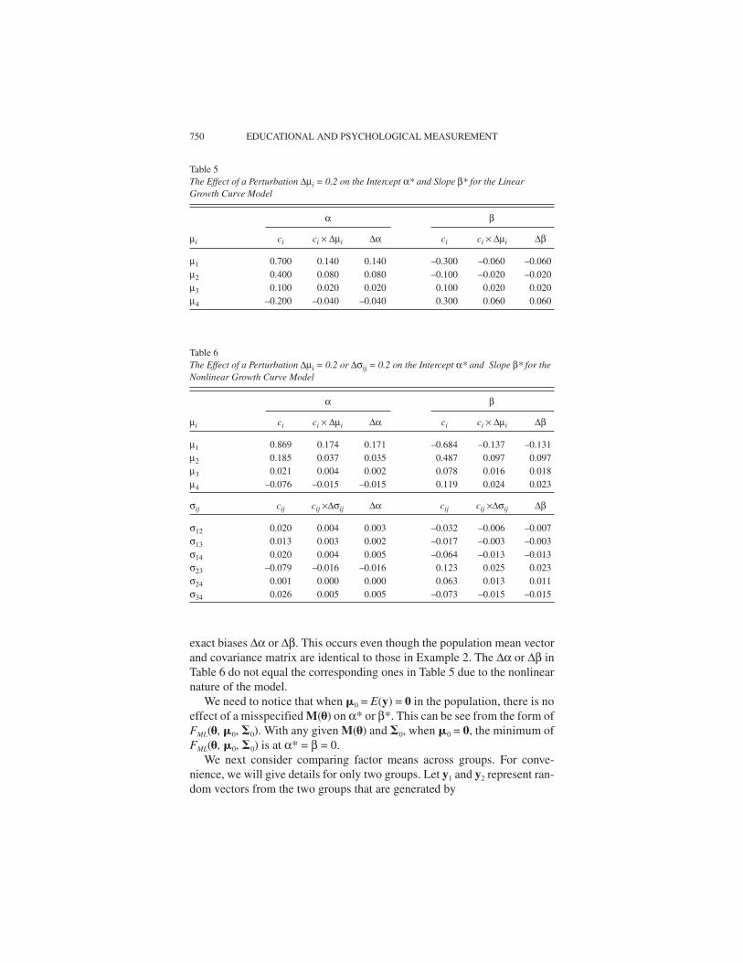
exact biases ∆α or ∆β. This occurs even though the population mean vectorand covariance matrix are identical to those in Example 2. The ∆α or ∆β inTable 6 do not equal the corresponding ones in Table 5 due to the nonlinearnature of the model.

We need to notice that when �0 = E(y) = 0 in the population, there is noeffect of a misspecified M(�) on α* or β*. This can be see from the form ofFML(�, �0, �0). With any given M(�) and �0, when �0 = 0, the minimum ofFML(�, �0, �0) is at α* = β = 0.

We next consider comparing factor means across groups. For conve-nience, we will give details for only two groups. Let y1 and y2 represent ran-dom vectors from the two groups that are generated by


Table 5The Effect of a Perturbation ∆ i = 0.2 on the Intercept α* and Slope β* for the LinearGrowth Curve Model

α β

µi ci ci × ∆µi ∆α ci ci × ∆µi ∆β

µ1 0.700 0.140 0.140 –0.300 –0.060 –0.060µ2 0.400 0.080 0.080 –0.100 –0.020 –0.020µ3 0.100 0.020 0.020 0.100 0.020 0.020µ4 –0.200 –0.040 –0.040 0.300 0.060 0.060

Table 6The Effect of a Perturbation ∆ i = 0.2 or ∆ ij = 0.2 on the Intercept α* and Slope β* for theNonlinear Growth Curve Model

α β

µi ci ci × ∆µi ∆α ci ci × ∆µi ∆β

µ1 0.869 0.174 0.171 –0.684 –0.137 –0.131µ2 0.185 0.037 0.035 0.487 0.097 0.097µ3 0.021 0.004 0.002 0.078 0.016 0.018µ4 –0.076 –0.015 –0.015 0.119 0.024 0.023

σij cij cij ×∆σij ∆α cij cij ×∆σij ∆β

σ12 0.020 0.004 0.003 –0.032 –0.006 –0.007σ13 0.013 0.003 0.002 –0.017 –0.003 –0.003σ14 0.020 0.004 0.005 –0.064 –0.013 –0.013σ23 –0.079 –0.016 –0.016 0.123 0.025 0.023σ24 0.001 0.000 0.000 0.063 0.013 0.011σ34 0.026 0.005 0.005 –0.073 –0.015 –0.015

y1 = 1 + �1f1 + e1 and y2 = 2 + �2f2 + e2, (5)

whose first two moment structures are

1(�) = 1 + �1�1, M1(�) = �1�1�1′ + �1,

2(�) = 2 + �2�2, M2(�) = �2�2�2′ + �2.

It is typical to assume 1 = 2 = and �1 = �2 = � in studying the mean differ-ence �2 – �1 (Sörbom, 1974). But there can be exceptions (Byrne, Shavelson,& Muthen, 1989). For the purpose of identification, one typically fixes �1 = 0,and consequently the interesting null hypothesis is H0 : �20 = 0. The free pa-rameters in Equation 5 are

� � � � � � �= ′ ′ ′ ′ ′ ′ ′ ′( , , , , , ) ,2 1 1 2 2,

where �, �1, �1, �2, and �2 are vectors containing the free parameters in �,�1, �1, �2, and �2. With the sample moments y1, S1, and y2, S2, the normaltheory-based MLE �� is obtained by minimizing

FML(�, y1, S1, y2, S2) = n–1n1FML(�, y1, S1) + n–1n2FML(�, y2, S2),

where n1 and n2 are the sample sizes for the two groups with n = n1 + n2. Understandard regularity conditions, �� converges to �*, which minimizes FML(�,�10, �10, �20, �20), where �10 = E(y1), �10 = Cov(y1), �20 = E(y2), and �20 =Cov(y2).

Notice that when the population parameter values satisfy �10 = �20 = �0,whether M1(�) and M2(�) are misspecified or not, the * has to take the value�0 and � 2

* has to be zero in order for FML(�, �10, �10, �20, �20) to reach its min-imum. So when �10 = �20 = �0, there will be no bias in � 2

* even when M1(�)and M2(�) are misspecified. The converse is also partially true. That is, when� �2 10

* ,≠ 0 will not equal 20 regardless of whether M1(�) or M2(�) are cor-rectly specified. This partially explains the results of Kaplan and George(1995) and Hancock, Lawrence, and Nevitt (2000) regarding the perfor-mance of TML in testing factor mean differences when factor pattern coeffi-cients are partially invariant. They found that TML performs well in control-ling Type I and Type II errors when n1 = n2, and it is preferable to other typesof analysis.

However, any misspecification will cause an asymptotic bias in �� 2 whenH0 is not true or when �10 ≠ �20. We illustrate how misspecified (1(�), M1(�))and (2(�),M2(�)) interfere with the estimate �� 2 and with testing the null hy-pothesis �20 = 0. Let �0 be the population value of � corresponding to cor-rectly specified models and � � �1

01 0 2

02 0 1

0= = =( ), ( ), M1 0( ),�� 2

02 0= M ( ). Similar to the one-group situation,� is a function of ( 1, �1, 2,


�2) in a neighborhood of ( � �10

10

20

20, , , ). For the ∆� = (∆θ1, . . . , ∆θq)′ =�* –

�0, we have

∆ ∆ ∆θ µ σli

p

j

p

i

p

cli iclij ij

≈ + += ==∑ ∑∑( ) ( ) ( ) ( ) ( )1 1

1

1 1

11

2

cli iclij iji

p

j

p

i

p( ) ( ) ( )2

1

2 2

11∆ ∆µ σ

= ==∑ ∑∑+ . (6)

Explicit expressions for cli li lijc c( ) ( ) ( )

, ,1 2 1

, and clij

( )2

are provided in Yuan andBentler (2004). Equation (6) can be used to evaluate the effect of anymisspecifications of (1(�), M1(�)) and/or (2(�), M2(�)) on �*, as illustratedin the following example.

Example 4

Let the population means and covariances be generated by Equation 5with four variables measuring one factor. We will use �1 and �2 to denote thevectors of factor pattern coefficients instead of their matrix versions �1 and�2. Set the population values

10 = 20 = (1.0, 1.0, 1.0, 1.0)′, τ10 = 0, τ20= 0.5, �10 = �20 = (1.0, 1.0, 1.0, 1.0)′,

φ φ ψ ψ ψ01

02

1101

4401

11021 0 1 0 1 0( ) ( ) ( ) ( ) (. , . , .= = = = =… and ) ( ) . .= = =… ψ 440

2 1 0

So the model in Equation 5 is correct for the population if there are no pertur-bations. Fix the first factor pattern coefficient at 1.0 for the purpose of identi-fication and let

�1 = �2 = (1, λ1, λ2, λ3)′

and τ1 = 0 in the model; the free parameters are

� = ′( , , , , , , , , ,( ) ( ) ( ) ( ) ( )τ λ λ λ φ ψ ψ ψ ψ2 1 2 31

111

221

331

441 , , , , , )( ) ( ) ( ) ( ) ( )φ ψ ψ ψ ψ2

112

222

332

442 ′.

Using Equation 6, with equal sample size in the two groups, we get the coeffi-cients ci and cij in the first column of Table 7 for the biases in τ2

* . With∆ ∆ ∆( ) ( ) ( )µ µ σi i ij

1 2 10 2 0 2 0 2= = =. , . , . and ∆ (2)σ ij = 0 2. , the approximatebiases using Equation 6 as well as the exact ones in τ2

* are given in the secondand third columns of Table 7, in which the approximate biases closely matchthe corresponding exact ones.

According to the coefficients in Table 7, any positive perturbation on µ i( )1

will cause a negative bias on τ2* , and the opposite is true when µ i

( )2 is posi-tively perturbed. Similarly, τ2

* will change in the direction specified by cij

when σij is perturbed. The results in Table 7 imply that one has to be cautiouswhen using a z test for τ20 = 0. When 10 and 20 are not equal, or the factor pat-


tern coefficients �10 and �20 are not invariant, or the structural models M1(�)and M2(�) are misspecified, the estimate �τ2 cannot be regarded as the esti-mate of the latent mean difference τ20. The bias ∆τ2 can be substantial. Justlike a nonzero parameter, the bias in �τ2 will be statistically significant whensample sizes are relatively large.

For the four examples in this section, we studied only ∆θl for a few inter-esting parameters when the mean µi or covariance1 σij are perturbed individu-ally. Equations 3 or 6 can also be used to obtain an approximate bias on any


Table 7The Effect of a Perturbation ∆ i = 0.2 or ∆ ij = 0.2 on the Difference τ 2

* of Factor Means inLatent Mean Comparison

µi ci ci × ∆µi ∆τ2

µ11( ) -0.314 -0.063 -0.059

µ21( ) –0.229 –0.046 –0.044

µ31( ) –0.229 –0.046 –0.044

µ41( ) –0.229 –0.046 –0.044

µ12( ) 0.314 0.063 0.066

µ22( ) 0.229 0.046 0.047

µ32( ) 0.229 0.046 0.047

µ42( ) 0.229 0.046 0.047

σij cij cij × ∆µi ∆τ2

σ121( ) 0.057 0.011 0.012

σ131( ) 0.057 0.011 0.012

σ141( ) 0.057 0.011 0.012

σ231( ) –0.057 –0.011 –0.015

σ241( ) –0.057 –0.011 –0.015

σ341( ) –0.057 –0.011 –0.015

σ122( ) 0.057 0.011 0.012

σ132( ) 0.057 0.011 0.012

σ142( ) 0.057 0.011 0.012

σ232( ) –0.057 –0.011 –0.015

σ242( ) –0.057 –0.011 –0.015

σ342( ) –0.057 –0.011 –0.015

parameter in a model with simultaneous perturbations on elements of meansand covariances. For example, when µ 1

1( ) and σ 342( ) are perturbed by

∆µ 11 0 2( ) .= and ∆µ 34

2 0 2( ) .= simultaneously, the approximate bias on τ2* is

about ∆τ2 = –0.314 × 2 – 0.057 × 2 = –0.074.

Discussion and Conclusion

When variables contain measurement errors, correlation or regressionanalysis might lead to biased parameter estimates. SEM supposedly removesthe biases in regression or correlation coefficients. However, if a model ismisspecified, the correlation or regression coefficients among latent vari-ables are also biased. Because the measurement errors are partialled out,SEM also has merits over the traditional MANOVA in comparing mean dif-ferences, as discussed in Cole, Maxwell, Arvey, and Salas (1993) and Kano(2001). However, this methodology can also be easily misused. In such acase, the estimated latent mean differences may not truly reflect the meandifferences of the latent variables.

There are many model fit indices in the literature of SEM. For example,SAS CALIS provides about 20 fit indices in its default output. Consequently,there is no unique criterion for judging whether a model fits the data. Con-ceivably, these different criteria might provide good resources because eachfit index may provide additional information for looking at the discrepancybetween data and model. Actually, Hu and Bentler (1999) recommendedusing multiple indices in judging the fit of a model. However, people in prac-tice often pick the most favorable index to sell a model. Particularly, with agiven fit index, the cutoff value between a good and a bad model is not clear;the commonly used terms adequate, plausible, or tenable for models havenever been defined clearly. For example, for the comparative fit index (CFI),the criterion CFI > 0.95 has been recommended for an acceptable model(Bentler, 1990; Hu & Bentler, 1999), but CFI > 0.90 is also commonly usedfor indicating adequate, plausible, or tenable models. It is interesting toobserve that fit indices are often used when judging a covariance structurebecause of the need to accept the model, whereas chi-squares or z tests aregenerally used when judging a mean difference because of the need to findsignificance (see Hong et al., 2003; Whiteside-Mansell & Corwyn, 2003).Such a practice most likely leads to misleading conclusions.

We agree that any model is an approximation to the real world and thatthere is some need to quantify the degree of approximation. But there aregood approximations and bad ones. As we have shown, if a significance or asubstantive conclusion following an SEM model is due to systematic biases,caution is needed in elaborating on the findings from the model. To minimizethe misuse of ∆T and z tests, one should use multiple criteria to make sure thebase model Ma is correctly specified. When Ma is not good enough, one may


need to find a different model structure that better fits the data before addingextra constraints or performing a z test. An alternative is to further explore thestructure of the data to better understand the substantive theory.

Our study leads to two humble but definite conclusions with regard to thespecific types of models. In the latent growth curve models as represented byEquation 4, when �α or �β is statistically significant at the .05 level, then with95% confidence one can claim that E(y) is different from zero. In comparingfactor means as represented in the model in Equation 5, if �� 2 is statisticallysignificant at the .05 level, then one can be 95% confident that E(y1) ≠ E(y2).But the significance in �α or �β may not be due to nonzero E(f1) or E(f2), and thesignificance of �� 2 may not be due to a nonzero E(f2 – f1).

Note

1. Tables 4, 6 and 7 do not contain σii

because its perturbation does not cause any biases onthe reported paramenters.

References

Bentler, P. M. (1990). Comparative fit indexes in structural models. Psychological Bulletin, 107,238-246.

Bollen, K. A. (2002). Latent variables in psychology and the social sciences. Annual Review ofPsychology, 53, 605-634.

Brouwers, A., & Tomic, W. (2001). The factorial validity of scores on the teacher interpersonalself-efficiency scale. Educational and Psychological Measurement, 61, 433-445.

Browne, M. W., & Arminger, G. (1995). Specification and estimation of mean and covariancestructure models. In G. Arminger, C. C. Clogg, & M. E. Sobel (Eds.), Handbook of statisticalmodeling for the social and behavioral sciences (pp. 185-249). New York: Plenum.

Buse, A. (1982). The likelihood ratio, Wald, and Lagrange multiplier tests: An expository note.American Statistician, 36, 153-157.

Byrne, B. M., Shavelson, R. J., & Muthen, B. (1989). Testing for the equivalence of factorialcovariance and mean structures: The issue of partial measurement invariance. PsychologicalBulletin, 105, 456-466.

Chou, C.-P., & Bentler, P. M. (1990). Model modification in covariance structure modeling: Acomparison among likelihood ratio, Lagrange multiplier, and Wald tests. Multivariate Be-havioral Research, 25, 115-136.

Cole, D. A., Maxwell, S. E., Arvey, R., & Salas, E. (1993). Multivariate group comparisons ofvariable systems: MANOVA and structural equation modeling. Psychological Bulletin, 114,174-184.

Curran, P. J. (2000). A latent curve framework for the study of developmental trajectories in ado-lescent substance use. In J. R. Rose, L. Chassin, C. C. Presson, & S. J. Sherman (Eds.),Multivariate applications in substance use research: New methods for new questions (pp. 1-42). Mahwah, NJ: Lawrence Erlbaum.

Drasgow, F., & Kanfer, R. (1985). Equivalence of psychological measurement in heterogeneouspopulations. Journal of Applied Psychology, 70, 662-680.

Duncan, T. E., Duncan, S. C., Strycker, L. A., Li, F., & Alpert, A. (1999). An introduction to latentvariable growth curve modeling: Concepts, issues, and applications. Mahwah, NJ: Law-rence Erlbaum.


Hancock, G. R., Lawrence, F. R., & Nevitt, J. (2000). Type I error and power of latent mean meth-ods and MANOVA in factorially invariant and noninvariant latent variable systems. Struc-tural Equation Modeling, 7, 534-556.

Hong, S. H., Malik, M. L., & Lee, M.-K. (2003). Testing configural, metric, scalar, and latentmean invariance across genders in sociotropy and autonomy using a non-Western sample.Educational and Psychological Measurement, 63, 636-654.

Hu, L. T., & Bentler, P. M. (1999). Cutoff criteria for fit indexes in covariance structure analysis:Conventional criteria versus new alternatives. Structural Equation Modeling, 6, 1-55.

Jöreskog, K. G. (1971). Simultaneous factor analysis in several populations. Psychometrika, 36,409-426.

Jöreskog, K. G. (1978). Structural analysis of covariance and correlation matrices.Psychometrika, 43, 443-477.

Kano, Y. (1986). Conditions on consistency of estimators in covariance structure model. Journalof the Japan Statistical Society, 16, 75-80.

Kano, Y. (2001). Structural equation modeling for experimental data. In R. Cudeck, S. H. C. duToit, & D. Sörbom (Eds.), Structural equation modeling: Present and future (pp. 381-402).Chicago: Scientific Software.

Kaplan, D. (1989). Power of the likelihood ratio test in multiple group confirmatory factor analy-sis under partial measurement invariance. Educational and Psychological Measurement, 49,579-586.

Kaplan, D., & George, R. (1995). A study of the power associated with testing factor mean differ-ences under violations of factorial invariance. Structural Equation Modeling, 2, 101-118.

Larose, S., Guay, F., & Boivin, M. (2002). Attachment, social support, and loneliness in youngadulthood: A test of two models. Personality and Social Psychology Bulletin, 28, 684-693.

Lawley, D. N., & Maxwell, A. E. (1971). Factor analysis as a statistical method (2nd ed.). NewYork: American Elsevier.

Lee, S. Y. (1985). On testing functional constraints in structural equation models. Biometrika, 72,125-131.

Lee, S. Y., & Leung, T. K. (1982). Covariance structure analysis in several populations.Psychometrika, 47, 297-308.

MacCallum, R. (1986). Specification searches in covariance structure modeling. PsychologicalBulletin, 100, 107-120.

MacCallum, R. C., & Austin, J. T. (2000). Applications of structural equation modeling in psy-chological research. Annual Review of Psychology, 51, 201-226.

Mardia, K. V., Kent, J. T., & Bibby, J. M. (1979). Multivariate analysis. New York: AcademicPress.

McArdle, J. J., & Epstein, D. (1987). Latent growth curves with developmental structure equa-tion models. Child Development, 58, 110-133.

Meredith, W., & Tisak, J. (1990). Latent curve analysis. Psychometrika, 55, 107-122.Satorra, A. (1989). Alternative test criteria in covariance structure analysis: A unified approach.

Psychometrika, 54, 131-151.Satorra, A., & Saris, W. (1985). Power of the likelihood ratio test in covariance structure analysis.

Psychometrika, 50, 83-90.Shapiro, A. (1984). A note on the consistency of estimators in the analysis of moment structures.

British Journal of Mathematical and Statistical Psychology, 37, 84-88.Sörbom, D. (1974). A general method for studying differences in factor means and factor struc-

tures between groups. British Journal of Mathematical and Statistical Psychology, 27, 229-239.

Steiger, J. H., Shapiro, A., & Browne, M. W. (1985). On the multivariate asymptotic distributionof sequential chi-square statistics. Psychometrika, 50, 253-264.


Vispoel, W., Boo, J., & Bleiler, T. (2001). Computerized and paper-and-pencil versions of theRosenberg Self-Esteem Scale: A comparison of psychometric features and respondent pref-erences. Educational and Psychological Measurement, 61, 461-474.

Whiteside-Mansell, L., & Corwyn, R. F. (2003). Mean and covariance structure analysis: An ex-amination of the Rosenberg Self-Esteem Scale among adolescents and adults. Educationaland Psychological Measurement, 63, 163-173.

Yuan, K.-H., & Bentler, P. M., (2004). Mean comparison: Manifest variable versus latent vari-able. Under review.

Yuan, K.-H., Marshall, L. L., & Bentler, P. M. (2003). Assessing the effect of modelmisspecifications on parameter estimates in structural equation models. Sociological Meth-odology, 33, 241-265.


ON CHI-SQUARE DIFFERENCE AND z TESTS IN MEAN …kyuan/courses/sem/readpapers/... · ON CHI-SQUARE...

Documents

Transcript of ON CHI-SQUARE DIFFERENCE AND z TESTS IN MEAN …kyuan/courses/sem/readpapers/... · ON CHI-SQUARE...