Abstract

ON A TRAVEL TIME ESTIMATION METHOD BASED ON AERIAL PHOTOGRAPHS

Author Institution

Adress

Author Institution

Adress

Country Commission Number

Yasuji Makigami Department of Civil Engineering Ritsumeikan University Kita-ku, Kyoto, Japan

& Masachika Hayashi Mineyama Construction Office Prefecture of Kyoto Mineyama-cho, Kyoto, Japan

Japan

V

In almost all the big cities, traffic congestion occurs widely on their expressway networks. In order to cope with the situ­ation, it is often required to make traffic surveys which cover a fairly long section of expressways. In this study, a mathematical method was developed to estimate the travel time along the long study section based on series of aerial photo­graphs and traffic volume measurements on two or more road side video camera recordings manking use of three dimensional representation of traffic flow. The method was applied to the results of traffic surveys conducted on the Hanshin Expressway as well as the Meishin Expressway.

1. Introduction Japanese Expressways in large urban areas are often tied up with increasing traffic demands and the traffic congestion is becoming worse every year. In order to cope with this situ­ation, highway authorities first need to grasp the traffic situation. It is especially important and effective to measure the Travel time along each expressway route in order to inves­tigate countermeasures for the traffic congestion. Two major methods are used to obtain travel time information. In one method the test vehicle is in the stream of traffic. In the second method, individual vehicles are followed by checking their number plates. However in the case of the first method, a great number of vehicles and drivers are needed to obtain travel time data to compensate for the long periods of traffic congestion. The second method can not monitor the fluctuations in speed along the expressway route, and the plate number travel time matching becomes very difficult in the case of a long section under study with heavy traffic demands. A recent method of input-output survey using test vehicles and continuous one minute volume count at both ends of the study section gives a good estimation of travel time fluctuation with time. However the method is not effectively applied to a study section with on and off ramps. This report describes an analytical travel time estimation method using aerial photographs and traffic volume counts. The method was developed based on the theory of three dimen­sional traffic flow presentation with three mutually perpen-

373

dicular axis of the time, the space and the accumulated number of vehicle arrivals.

2. The three dimensional representation of traffic flow and the traffic surface.

It is possible to represent traffic flow as a three dimen­sional stepwise surface with three mutually perpendicular axis of the time (t), the space (x) and the accumulated number of vehicle arrivals (n) (hereafter refered to accumulated arri­vals) as shown in reference 5. The stepwise traffic surface is depicted by conbining the usual vehicle trajectories on the time-space field with the third axis of the accumulated arri­vals perpendicular to the time space field. The stepwise tra­ffic surface can be regarded to be smoothed off to a continu­ous even surface when hundreds of vehicle trajectories are ob­served like usual traffic surveys. Let the traffic surface corresponding to the domain An on the t-x plane be traffic surface A as shown in Fig. 1. In addition, let Ax and At be the projection of the traffic surface A to the n-t plane and the n-x plane respectively also as shown in Fig. 1. Then the average tra­ffic volume (q), the average tra­ffic density (k) and the average running speed within the time­space domain An are given by the following equations. q = At/An, k = Ax/An, v = At/Ax ...... (1) The travel time estimation method based on the theory of the three dimensional traffic surface was developed under the assumptions concerning traffic and roadway conditions and the traffic sur­vey method shown below.

I

n -Cumulative Number of Vehicles

FIG. 1 - Traffic Surface and Its Projections

i) The estimation method is applicable only to a section of divided access-controlled expressway. Attention is to be given only to one directional traffic stream.

ii) Assumed survey methods are; (a) series of aerial photo­graph taking and (b) continuous traffic volume counts from roadside measuring stations. Every series of aerial photographs covers all the vehicles observed on the ex­pressway during each flight period. Two or more mainline volume count stations are supposed to be located along the study section with additional count stations on each on and off ramp terminal. It is also assumed that the arrival time of all the vehicles are recorded at no less than two mainline count stations.

With the aerial photographs and traffic volume counts describ­ed above, the flight trajectories for the aerial photograph taking and the accumulate darrivals atthe main line count sta­tions are fixed on the traffic surface defined by the study section and the traffic survey period (see Fig.2). Attention should be given to the method of estimating the position and

374

the slope of an arbitrary po rtion of the tr affic sur face. For instance, defined by an arbitrary section from Xl to X2, and an arbitrary period from tl to t 2 .

3. Traffic Volume Fluctu­ation Limit and Estima­tion of Traffic Flow Characteristics.

n Cumulative Number of Vehicles Traffic Surface

Let n(xl,t l ) be the accu­mulate arrivals at an ar­bitrary point Xl in the study section and at arbi­trary time t 1. The value of n (x 1 t 1) can bee s t i -mated from the accumulated FIG.! Trlffic Surflce Ind traffic Suney arrivals on the flight lines passing point Xl before and after time (td. Assuming that the two flight lins are to be those of the ~th and the (~+l )th flight respectively, let t~(XI) and n~(xI) be the passing time of point Xl of the ~th flight and the accumulated arrivals at point Xl on the ~th flight line. Then the difference of the point Xl passing time of the ~th flight and the (~+l)th flight; t~+I(XI)' and the hourly traffic flow rate at point Xl during that period; q~+I(Xl) are given by the following equations.

~+l ~+l ~ t9J (X.l) t (Xl) - t (Xl) }

q~+l(xd [n~+l(xd _ n9.(xl)] /t~+l(xd ............. (2)

Now, the estimation of traffic density {k~+I(XI)} is given by the following equation:

~+l ~+l ~ ~ k~+I(XI) = ~[n (xo)-n (X2) n (xo)-n (X2)] ...... (3) ~ 2 X2- XO X2- XO

where points Xo and X2 are arbitrary points located upstream and downstream of point Xl respectively. Those values are es­timations of the traffic volume and density at poin (Xl, tl) on the time-space field under the given flight line and volume count conditions. Therefore, those values are not determinis­tic but show probablistic fluctuations. Following is a description of the method of how to estimate the fluctuation range of the traffic volume and density. Sup­pose that it is possible to estimate the variance of vehicle arrivals during a short time interval of the order of two to five seconds by analysing the data from the arrival time recording mainline count stations. Let ot(XI' tl) be the var­iance of vehicle arrivals during time interval T at the point (Xl, tl) on the time-space field. If it is supposed that ve­hicle arrivals fluctuate independently, then from the central limit theory, it is possible to consider that the accumulation of vehicle arrivals at point Xl and time tl has a normal dis­tribution as shown below.

375

n(X1, tl)'tJ Q, Q,+l Q,+l Q,+l /] N[{n (X1)+~tQ, (Xl)"qQ, (Xl)}'02(tl,Xl)·~tQ, (Xl) T (4)

h Q,+1 . Q,+1 Q,] W ere ~ t Q, (X 1) = m l n [ t (X 1 ) - t 1, t 1 - t (X 1) ••••••••••• (5 ) It should be noted that equation (4) is for the case where

{tQ,+l(Xl)-tl ~ tl-tQ,(Xl)} Now, let an be the reliability co-efficient with degree of re­liability of n%, and further let max nn(x1, tl) and min nn(xl, tl) be the upper and the lower limit of n(xl, tl) with n% re-liability. Then under the samecondition as equation (4),

Q, Q,+1 Q,+l = n (Xl)+~tQ, (Xl) oqQ, (Xl) max n n (x 1, t 1) I min nn(x1, tl) j ~+l

±an0(xl, t 1) ~tQ, (X1)/T ..... (6)

Fig. 3 shows the fluctuation of the upper and the lower limit of the accumulated arrivals at point Xl. (2) Estimation of Traf­

fic Flow Character­istics

Following the above ar-

n Cross Section of Traffic Surface

1+1 gument, the upper and n (xIJl---------------:;jiJ(

the lower limits of accumulated arrivals within the time-space field An defined by section Xl 'tJ X2 and in­terval t 1 'tJ t 2 stay within such three di­mensional domains as shown in Fig. 4 a or b. (The three dimensional domain is refered to as n limit domain here­after) Now according to the definition shown in Fig. 1, let the average and the upper and lower value of the area of the projection of traf­fic surface A (x 1 'tJ X 2 , t 1 'tJt 2) to the n-x pla~e and the n-t plane

tl R.+l tl I--____ t R. (x 1)

tR.CxIJ Flight Line R.

tR.+ICXr}

Flight Line(R.+l)

FlG.3 Fluctuation of the Upper and the Lower

Limit of the Accumulated Vehicle Arrivals.

be At(Xl 'tJX2,t l 'tJt 2), max At(Xl 'tJX2, tl 'tJt2) and min At(Xl 'tJX2 , tl 'tJt 2) as well as AX(XI 'tJX2, t1 'tJt2), max AX(XI 'tJX2, t1 'tJt2 ) and min AX(X1'tJX2, t l 'tJt2) respectively. Then from equation (1), the average traffic volume q(X 1'tJX2, t1'tJt2) is given by the following equation:

At(X I'tJX2, t1'tJt2) q(X 1'tJX2, t1'tJt2) =

An (X 1'tJX2, t l 'tJt 2)

[{fl(Xl, t 2)-n(Xl,t 1)}-{n(X2, t2)-n(X2' tl)}] (X2- Xl) ---------------------------------------------------------... 2(X2- XI) .(t2-tl)

376

( 7)

The traffic surface posi­tion that makes At(Xl 'VX2, t 1 'V t 2) maximum is the posi­tion which makes the traf­fic surface slope along the time axis maximum and the traffic surface position that makes At(Xl 'V X2 ,tl 'V t2) minimum is the position which makes the traffic surface slope minimum. Therefore the maximum and the minimum rate of traffic volume, max q(Xl'V X2 ,tl 'V t2) and min q(Xl'V X2, tl'V t2), are given by the following equations:

x

FIG.4 Limit Domain 01 Traffic Surface

Corresponding to Field An (X,- Xl • It- td

max At(X l 'VX2, t l 'Vt2)

An(X l 'VX2, t l 'Vt 2)

min At (x 1 'VX 2, t 1 'Vt 2 ) • • • • • • • •• ( 8 )

An(X l 'VX2, t 1 'Vt2)

In the above equations, such detailed expressions for computa­tion purposes as shown at the end of equation (7) are abbrevi­ated. Equations for traffic density calculation can be de­rived in the same manner and the results are as follows.

AX(X 1 'VX 2, t 1 'Vt2) k(Xl'VX2' t 1 'Vt2) =

An(X 1 'VX2, t 1 'Vt2)

max AX(X 1 'VX2, t 1 'Vt2) max k(xl'Vx2' t 1 'Vt2) =

An(x 1 'Vx2, t 1 'Vt 2)

min AX(X l 'VX2, t 1 'Vt2) min k(xl,,-,x2, t 1,,-,t 2) =

An(X 1 'VX2, t l 'Vt2)

. . . . . . .. ( 9)

Where k (x 1 'V X 2, t 1 'V t 2), max k (x 1 'V X 2, t 1 'V t 2) and min k (x 1 'V X2, tl'V t2) are the average, the maximum and the minimum value of traffic density that can be expected within the limit domain respectively. From the third equation of equation (1), the average traffic speed, V(Xl 'V X2, tl'V t2), is calculated using the first equa­tion of equation (7) and (9).

377

At(X 1 "vX2, t 1 "vt 2)

AX(X 1 "vX2, t 1 "vt2) . . . . . . . . . . . . . . . . .. ( 1 0 )

t maximum and the minimum value of the avarage speed, max V(XI "v X2, t 1 "v t2) and min V(Xl"v X2, t 1 "v t2), can not be derived by s placing max At(x1"v X2, tl"v t2) in the numerator and min (Xl "v X2, t 1 "v t2) in the denominator or vice versa because, a traffic surface has a gradient that makes At (X 1"vX2, tl "v t 2) maximum within the n limit domain, it is impossible to give an additional slant to the traffic surface in order to make (x 1 "v X 2, t I "v t 2) minimum. There fore thos e upper and lower 1 ts of traffic speed can be shown as follows.

max [ max At(X 1 "vX2, t 1 "vt2)

]

.. (11)

min At(X I "vt2, t 1 "vt2) At(X 1 "vX2, t 1 "vt2)

AX(X 1 "vX2, t 1 "vt2) ,max AX(X 1 "vX2, t 1 "vt2)

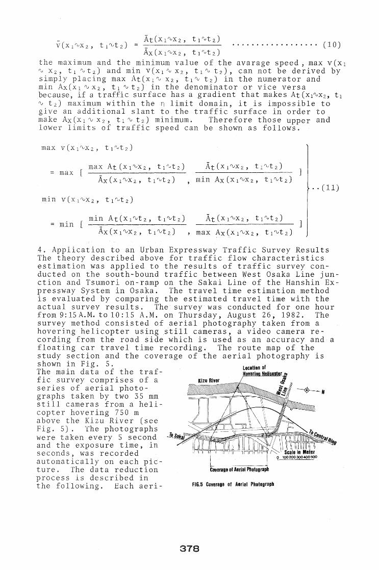
4. Application to an Urban Expressway Traffic Survey Results The theory described above for traffic flow characteristics estimation was applied to the results of traffic survey con­ducted on the south-bound traffic between West Osaka Line jun­ction and Tsumori on-ramp on the Sakai Line of the Hanshin Ex­pressway System in Osaka. The travel time estimation method is evaluated by comparing the estimated travel time with the actual survey results. The survey was conducted for one hour from 9: 15 A.M. to 10: 15 A.M. on Thursday, August 26, 1982. The survey method consisted of aerial photography taken from a hovering helicopter using still cameras, a video camera re­cording from the road side which is used as an accuracy and a floating car travel time recording. The route map of the study section and the coverage of the aerial photography lS shown in Fig. 5. The main data of the traf­fic survey comprises of a series of aerial photo­graphs taken by two 35 mm still cameras from a heli­copter hovering 750 m above t Kizu River (see Fig. 5) The photographs were taken every 5 second and the exposure time, in seconds, was recorded automatically on each pic­ture. The data reduction rocess is described in

t llowing. Each aeri-

location of

i.- -~j Coverage of Aerial Photograph

FIG.5 Coverage of Aerial Photograph

al exposure, on slide film, was projected on to a piece of white paper and all vehicles in each traffic lane were numbered, from downstream to upstream. The position of each vehicle was then noted on the paper and determined by measuring the distance between that vehicle and the nearest hundred-meter post using an

To Tamade

It P 3.20 3.25 3.30 3.35 3.40 3.45 3;50 3.55 3.60 3.65 3.70 3.75 3.80 3.85 3.90 3.95 4.00 A.IV! I

9: 40--,-----,,= -----;---,----,--,----,----,--.----i--,---

Traffic Density in Vehicles/ Kilometer

_140-

Ii.! 120-140

FIG.6 Density Contour Diagram from Computer Output

C=:J 100 -120

C=:J 0 -100

appropriate scale ruler. All the data was then tabulated for each lane. Every exposure was recorded on a magnetic tape for computer processing for the traffic volume, traffic density and running speed computation. Fig. 6 shows the traffic den­sity contour diagram depicted based on the output from the computer. Fig.? shows the five minute volume fluctuation with time. (2) Comparison of

the estimated and the measu­

red travel time. The estimation of the travel time using equation 10 and 11 is now com­pared with the travel time meas­urement. The

ID 220

~ .200 o II!: =- ~ 180 .!:! ... :;; 1.160 ... ID ~ .... 'ii 1401 ID - <

Shoulder Lane ; ........

""','.-------~-------"", --;~"""'Ii;,,; .. "'................. .. ___ ~---- ... -- .. ._._--------------- ""...:::..~~ ___ ___ -- ..... ..:,....c:=--:.~:-~------

:; ;! 1201 .: - ;y IE ~9:=15~9.:-..:2=-0-9:25- 9:30· 9:35 9:40 9:45 9:50 9:55 10:00 10:05 10:10 10:15 ID :a-

Li::: Time of the Day FIG.7 Five Minute Volume Fluctuation with Time

estimation theory described in section 3 was developed for a considerably long section using a series of aerial photographs taken from a fixed wing airplane as basic data. However, in order to evaluate the validity of equation 10 and 11 which compute the average and the fluctuation range of the running speed in 9 homogeneous section, investigation is concentrated on a 400 meter section from the 3.5 km post to the 3.9 km post within the aerial photograph coverage. The section is between the merging taper end of the West Osaka Line Junction and the ramp nose of Tsumori on-ramp and has a unform cross-section element with two traffic lanes. A 24 minute period from 9:46 A.M. to 10:10 A.M. was selected for the investigation and seven flight lines were assumed to run parallel with the time axis with three minute time intervals. That is, the traffic surface within a 400 meter section length and 3 minute time period was prepared for the evaluation. The number of vehi­cles along each flight line and the vehicle arrival numbers

both at the downstream and upstream end of the section were measured from trajectory diagrams in the time-space field, which is one of the outputs from the computer process de­scribed in the previous section. Then the position of the unit traffic surface in the three dimensional space was deter­mined. Therefore, the average and the maximum and minimum speed can be computed through equation (10) and (11) assuming a one and half minute evaluation range on both sides of each flight line. The estimated travel time can also be evaluated. The variance of vehicle arrivals can be calculated from the one minute traffic volume measurements at the upstream and downstream end of the 400 meter investigation section. The actual travel time through the 400 meter section can be ob­tained by measuring the arrival time at the upstream and down­stream ends of the 400 meter section following the trajectory of each vehicle. The travel time was measured with a sampling rate of one to five.

Table 1 summarizes the results of validation analy­sis. It shows the average, the vari­ance and the upper and the lower level with a 95 percent confidence level of the trav­el time contrasted with the estimated average and the estimated upper and lower limit value for each time interval. The summary table indicates that the estimated travel time agrees with travel time meas­urements fairly well except the time interval from 9:50;30 to 9:53;30 which is an unuse­al time interval because a truck proceeded with very s low speed for

Table-l Results of Validation

Time Interval Estimation Actual Data Variance

9:47.30- 42.0 39.3 35.2 34.2 ( 2.59) 9:50.30 30.1 29.2

9:50.30- 38.2 55.1 32.1 39.1 ( 8.17) 9,: 53.30 27.8 23.1

9:53.30- 44.9 48.2 37.4 36.1 ( 6.17) 9:56.30 32.0 24.0

9:56.30- 51.8 67.3 43.0 46.3 (10.71) 9:59.30 36.6 25.3

9:59.30- 55.7 53.8 46.5 45.4 ( 4.30) 10;02.30 39.8 37.0

10:02.30- 60.2 53.5

10:05.30 49.9 47.0 ( 3.33) 42.7 40.4

10:05.30- 59.6 54.2 49.7 47.0 ( 3.64) 10:08.30 42.5 39.9

Upper Level Average + 1.960' Estimated average Average

Lower Level Average - 1.960'

highway maintenance imspection. The coefficient of corre­lation between the actual and estimated travel time for the six time intervals is 0.89, indicating a good correlation.

5. Application to a Rural Expressway 5-1 Outline of traffic 'Survey In this section, attention is given to the application of the

380

travel time estimation theory to an actual expressway with a sizable length. The traffic survey selected for this purpose was the survey conducted on the southbound traffic between Kyoto South Interchange and Ibaraki Interchange on the Meishin Expressway during two hours from 9:30 A.M. to 11:30 A.M. on August 26th 1981. The three major methods of the survey were aerial photography, video recording and test vehicle running. The outline of the survey method and their results are as follows:

i) Video recording. In order to obtain data about the traf­fic volume fluctuation range and capacity, video recording was conducted at the middle and the end of a creeper lane; at upstream portals of tunnels as well as at a point representative of a flat section.

ti) Floating survey. Travel time and running speed were measured by the test vehicle floating method, recording passage time at each 200 meter post with 15 minute intervals.

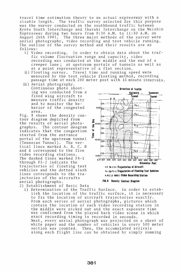
ill) Aerial photography. Continuous photo shoot­ing was conducted from a fixed wing aircraft to measure traffic density and to monitor the be­havior of the congested area.

Fig. 8 shows the density con­tour diagram depicted from the results of aerial photo­graphys. The contour deogram indicates that the congestion = started from the entrance E

Direction of Traffic

========,=====,==~K~ajiwar.=a ~A~~Tennozan Tunnel Tunnel ° E

i= po r t a I 0 f the ups t ream t unn e 1 10:30~~;r.t;I':t1~:A:i~~~~--+f=f=='----!-(Tennozan Tunnel). The ver­tical lines marked A. B. C. D and E correspond to the five video recording stations. The dashed lines marked F4-1 through F5-2 indicate the trajectories of floating test vehicles and the dotted slash lines corresponds to the tra­jectories of the aircrafts aerial photographs. 2) Establishment of Basic Data

C4 to C12; Trajectories of Aircraft F4-1 to F5-2; Trajectories of Floating Test Vehicles

A,B,C,D and E; Video Recording Station

FIG.8 Density Contour Diagram

i) Determination of the Traffic Surface. In order to estab­lish the location of the traffic surface, it is necessary to fix the location of aircraft trajectories exactly. From each series of aerial photographs, pictures which contain the location of each video recording station in the middle were picked out and the exact exposure time was confirmed from the played back video scene in which exact recording timing is recorded in seconds. Next, every aerial photograph was projected on a sheet of white paper and the number of vehicles in every 500 meter section was counted. Then, the accumulated arrivals along each flight line can be obtained by simply summing

381

up the vehicle numbers from the upstream end. The accum­lated arrivals along the time axis at each video recording station can be obtained by counting vehicle arrivals from the played back video. Then it is possible to establish the position of the traffic surface from the accumulated arrivals along the two different series of lines on the time space field.

) Estimation of traffic flow fluctuation characteristics The distribution of vehicle arrivals in a given time pe­riod is often best described by the Generalized Poison Distribution. Suppose m is the mean number of vehicle arrivals during the given period. Then the Generalised Poison Distribution is given by the following equation,

kp e - AT.

Pen) = 11 (nokp+i-l)!

1 where A = mokp + Z(kp-L)

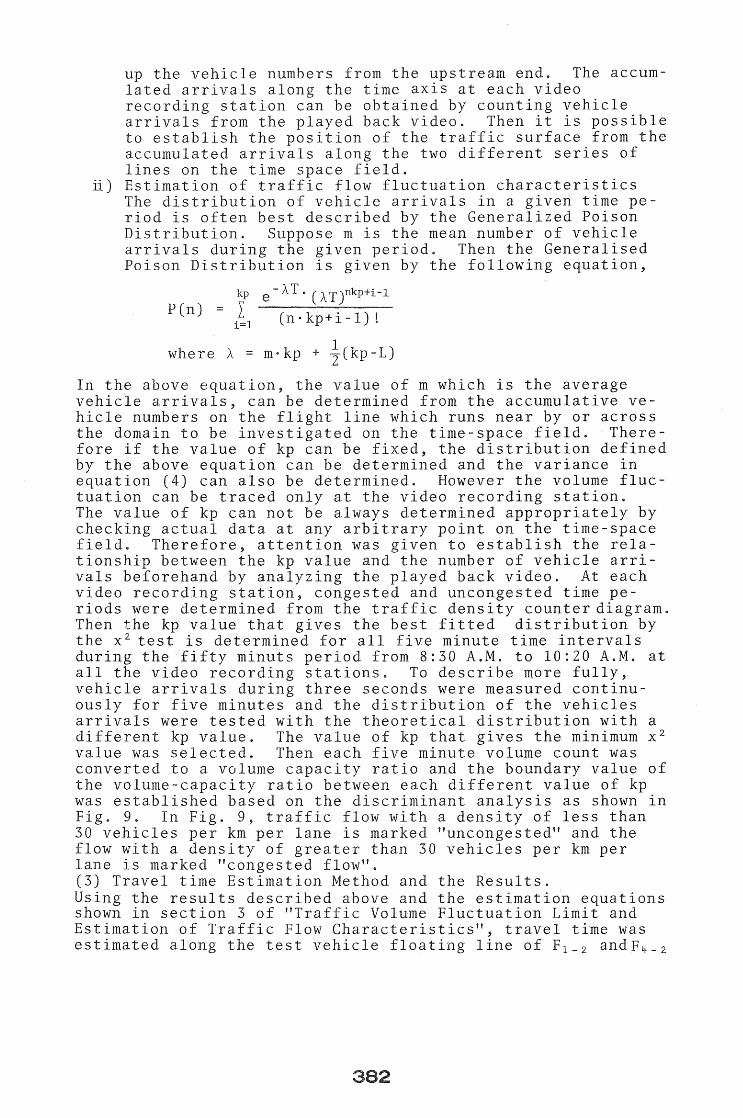
In the above equation, the value of m which is the average vehicle arrivals, can be determined from the accumulative ve­hicle numbers on the flight line which runs near by or across the domain to be investigated on the time-space field. There­fore if the value of kp can be fixed, the distribution defined by the above equation can be determined and the variance in equation (4) can also be determined. However the volume fluc­tuation can be traced only at the video recording station. The value of kp can not be always determined appropriately by checking actual data at any arbitrary point on the time-space field. Therefore, attention was given to establish the rela­tionship between the kp value and the number of vehicle arri­vals beforehand by analyzing the played back video. At each video recording station, congested and uncongested time pe­riods were determined from the traffic density counter diagram. Then the kp value that gives the best fitted distribution by the x 2 test is determined for all five minute time intervals during the fifty minuts period from 8:30 A.M. to 10:20 A.M. at all the video recording stations. To describe more fully, vehicle arrivals during three seconds were measured continu­ously for five minutes and the distribution of the vehicles arrivals were tested with the theoretical distribution with a different kp value. The value of kp that gives the minimum x 2

value was selected. Then each five minute volume count was converted to a volume capacity ratio and the boundary value of the volume-capacity ratio between each different value of kp was established based on the discriminant analysis as shown in Fig. 9. In Fig. 9, traffic flow with a density of less than 30 vehicles per km per lane is marked "uncongested" and the flow with a density of greater than 30 vehicles per km per lane is marked "congested flow". (3) Travel time Estimation Method and the Results. Using the results described above and the estimation equations shown in section 3 of "Traffic Volume Fluctuation Limit and Estimation of Traffic Flow Characteristics", travel time was estimated along the test vehicle floating line of F l _ 2 andF 4 _ 2

which are completely sur­rounded by the aerial pho-

6

5

tograph aircraft flight lines and the video recording time lines as shown in Fig. 8. The ::4 sec t io n in v est i gat e dis a 4. 4 = kilometer length section ~3 from the 506.0 to the 501.6 kilometer post. The section was divided into nine subsections with a length of 400 meter at the upstream subsection and 500 meters lengths for the rest of the subsections.

2

o \

Uncongssted Flow

0.70 0.75 0.80 0.85 0.90

Volume/ Capacity Ratio

FIG.9 Result of Discriminant Analysis for Kp Valus

A ten minute time interval was assumed for the estimation pe odD Then the average, the maximum and minimum travel t for t upstream first subsection can be obtained with travel speed computed from equation 10 through 11. The travel time compu­tation is then applied to the next downstream subsection taking the ten minute time interval with the time shift equal to the travel time through the first section. The procedure was continued subsection by subsection to the downstream end

Fig. 10 shows the maximum and the minimum travel time accumulation with the tra­jectory of test vehicle F l - 2

and F 4 - 2 o

Although there are some devi­ations between the actual trajectories and the esti­mated travel time accumu­lation on the intermediate subsections due to each test. vehicles driv­ing conditions,

660[

600

I 540t

480

-g 420 11:1 u GIl Y.I

360 .: ~300 j::

~240 ~ I-

180

120

505·0 1

504.0 2

503.0 502.0 3 4

660

600

540

480

420

360

300

240

180

501.0 K.P. 506. 5 K.M. 0

505.0 504.0 1 2

FIG.lO Estimated and Aetllal Trallel Ii me

503.0 3

502.0 4

501.OK.P. 5 K.M.

the travel time through the whole investigation section stays between the minimum and the maximum travel time estimation. This is because the upstream and the downstream ends of the 4.4 kilometer investigation section was definitely located in the three dimensional space of traffic surface by the video recording stations and the flight lines.

6. Conclustion The travel time on a fairly long expressway section was esti­mated from roadside video recording and a series of aerial photographs making use of the three dimensional traffic flow repre­sentation theory. The results of estimation are quite reasonable although there are some discrepancies between the actual and the estimated values when traffic flow is disturbed. For example, by very slow moving vehicles such as maintenance crew trucks, or when a series of aerial photographs did not completely record all the vehicles on the expressway. Attention should be given to accumulation of traffic surveys of this kind to increase the reliability of the estimation method.

References 1) Yasuji Makigami, G.F. Newell; Three-Dimensional Respresen­

tation of Traffic Flow, Transportation Science, Vol.S, No.3, p.302~313, August 1971.

2) Hanshin Expressway Public Corporation; Report on Traffic Congestion and Countermeasures on Hanshin Expressway Net­work, March, 1981.

3) Metropolitan Expressway Public Corporation; Report on Tra£­fic Survay for Metropolitan Expressway Route 6 and Katsu­shika-River Line, March, 1981.

4) Yasuji Makigami, Hamao Sakamoto and Masachika Hayashi; An Analytical Method of Traffic Flow Using Aerial Photographs, Journal of Transportation Engineering ASCE, Vol. 111, No.4, July, 1985.

384