On a Stochastic Representation Theorem for

Meyer-measurable Processes and its Applications in

Stochastic Optimal Control and Optimal Stopping

Peter Bank1 David Besslich 2

October 22, 2018

Abstract

In this paper we study a representation problem first considered in a simpler ver-sion by Bank and El Karoui [2004]. A key ingredient to this problem is a randommeasure µ on the time axis which in the present paper is allowed to have atoms.Such atoms turn out to not only pose serious technical challenges in the proof of therepresentation theorem, but actually have significant meaning in its applications, forinstance, in irreversible investment problems. These applications also suggest to studythe problem for processes which are measurable with respect to a Meyer-σ-field thatlies between the predictable and the optional σ-field. Technically, our proof amountsto a delicate analysis of optimal stopping problems and the corresponding optimaldivided stopping times and we will show in a second application how an optimal stop-ping problem over divided stopping times can conversely be obtained from the solutionof the representation problem.

Keywords: Representation Theorem, Meyer-σ-fields, Divided stopping times, OptimalStochastic Control.

1 Introduction

In this paper we study a stochastic representation problem, first considered in a simplerframework by Bank and El Karoui [2004]. Specifically, we consider a Meyer-σ-field Λ suchas the predictable or optional σ-field and, under weak regularity assumptions, construct aΛ-measurable process L such that a given Λ-measurable process X can be written as

XS = E

[∫[S,∞)

gt

(supv∈[S,t]

Lv

)µ(dt)

∣∣∣∣∣FΛS

](1)

at every Λ-stopping time S.In Bank and El Karoui [2004], stochastic representations like (1) are proven for op-

tional processes X and atomless optional random measures µ with full support. OurMain Theorem 2.16 generalizes their result in several ways. Most notably, we solve therepresentation problem for measures µ with atoms. Such atoms not only pose consider-able technical challenges for the representation problem (1), but also convey significantmeaning in its applications.

1Technische Universitat Berlin, Institut fur Mathematik, Straße des 17. Juni 136, 10623 Berlin, Ger-many, email bank@math.tu-berlin.de.

2Technische Universitat Berlin, Institut fur Mathematik, Straße des 17. Juni 136, 10623 Berlin, Ger-many, email besslich@math.tu-berlin.de.

1

arX

iv:1

810.

0849

1v1

[m

ath.

PR]

19

Oct

201

8

For instance in an application of this representation problem to a novel version of thesingular stochastic control problem of irreversible investment with inventory risk (see Bankand Besslich [2018c] and, e.g., Riedel and Su [2011], Chiarolla and Ferrari [2014] for earlierversions), µ and g are used to measure the incurred risk and the atoms of µ reflect timesof particular importance for the risk assessment; the process X describes the revenue peradditional investment unit. As proven in the companion paper Bank and Besslich [2018c],it then turns out that (supv∈[0,t] Lv)t≥0 yields an optimal investment strategy. At anyatom of µ, the optimal control has to trade off an improvement in the impending riskassessment against any revenue from additional investment. How exactly this comes downalso depends crucially on what information is available to the controller in this moment.This can be modelled by a Meyer-σ-field interpolating between “reactive” predictablecontrols and “proactive” optional ones; see Lenglart [1980] for a detailed account. Toaccount for the full variety of such information dynamics, we solve (1) for an arbitraryMeyer-σ-field Λ instead of merely the optional σ-field. Another extension over Bank andEl Karoui [2004] is the possibility to take every stopping time T instead of T = ∞ asthe time horizon in (1), not just predictable ones: We just need to “freeze” the problem’sinputs as we reach T . Moreover, we are able to prove that our solution L is maximalin the sense that any other Λ-measurable solution is less than or equal to ours up to anevanescent set. Instead of this natural maximality property, Bank and El Karoui [2004]just prove uniqueness under additional assumptions on the paths of L which do not alwaysobtain.

The technical challenges in establishing the representation (1) arise first due to the factthat the original construction of L in Bank and El Karoui [2004] is based on the propertiesof optimal stopping times for the family of auxiliary stopping problems

Y `S = ess sup

T∈S Λ([S,∞])

E

[XT +

∫[S,T )

gt(`)µ(dt)

∣∣∣∣∣FΛS

], ` ∈ R, S Λ-stopping time. (2)

When µ has atoms, the running costs can exhibit upward and downward jumps and so,optimal stopping times for (2) may exist only in the relaxed form of divided stopping times(or temps divisees, see El Karoui [1981]). Divided stopping times are actually quadruplesconsisting of a stopping time and three disjoint sets decomposing the probability space.These require a considerable more refined analysis. Conversely, we show that a solution to(1) also allows us to solve such generalized stopping problems and thus offers an alternativeto the usual approach via Snell envelopes as in El Karoui [1981].

While conceptually very versatile for modelling information flows and technically con-venient to unify the treatment of predictable and optional settings, the consideration ofMeyer-σ-fields adds mathematical challenges of its own. For instance, the level passagetimes of a Meyer-measurable process may not necessarily be Meyer stopping times: Theentry time of a predictable process is itself not predictable in general. Second, for op-tional processes, right-upper-semicontinuity in expectation implies pathwise right-upper-semicontinuity; see Bismut and Skalli [1977]. For Λ-measurable processes however, thisimplication does not hold true in general. Such subtleties can be disregarded when µ doesnot have atoms as in Bank and El Karoui [2004], but become crucial for (1) when it does.

This paper will be organized in the following way. Section 2 introduces the frameworkand the main result. In Section 3 we give applications of the main theorem first in

2

irreversible investment and then in optimal stopping over divided stopping times. InSection 4 we prove maximality and in Section 5 we finally prove existence of a solution Lto (1). The technical proofs of auxiliary results are deferred to the appendix.

2 A Representation Problem

Let us fix throughout a filtered probability space (Ω,F,F := (Ft)t≥0,P) and F∞ :=∨t Ft ⊂ F and F satisfying the usual conditions of completeness and right-continuity.

Furthermore let Λ be a P-complete Meyer-σ-field which contains the predictable-σ-fieldwith respect to F and is contained in the optional-σ-field with respect to F . We will usethe concept of Meyer-σ-fields as they can be used to model different information dynamicsin optimal control problems (see our companion paper Bank and Besslich [2018c]). ButMeyer σ-fields also allow us to prove our main result simultaneously for the predictable andthe optional-σ-field which are both special cases of Meyer-σ-fields. The theory of Meyer-σ-fields was initiated in Lenglart [1980]. We review and expand some of this material inthe companion paper Bank and Besslich [2018b]. Let us recall in the next Section 2.1 thebasic concepts and results. Upon first reading, the reader is invited to think of Λ as theoptional-σ-field in which case Λ-stopping times S Λ are just classical stopping times andmay then skip directly to Section 2.2.

2.1 Meyer-σ-fields

Definition 2.1 (Meyer-σ-field, Lenglart [1980], Definition 2, p.502). A σ-field Λ on Ω×[0,∞) is called a Meyer-σ-field, if the following conditions hold:

(i) It is generated by some right-continuous, left-limited (rcll or cadlag in short) pro-cesses.

(ii) It contains ∅,Ω×B([0,∞)), where B([0,∞)) denotes the Borel-σ-field on [0,∞).(iii) It is stable with respect to stopping at deterministic time points, i.e. for a Λ-

measurable process Z, s ∈ [0,∞), also the stopped process (ω, t) 7→ Zt∧s(ω) is Λ-measurable.

Example 2.2. The optional σ-field O(F ) and the predictable σ-field P(F ) associated toa given filtration F are examples of Meyer-σ-fields.

Like for filtrations, there also exists a notion of completeness of Meyer-σ-fields withrespect to a probability measure P:

Definition and Theorem 2.3 (P-complete Meyer-σ-field, see Lenglart [1980], p.507-508).A Meyer-σ-field Λ ⊂ F⊗B([0,∞)) is called P-complete if any process Z which is indistin-guishable from a Λ-measurable process Z is already Λ-measurable. For any Meyer-σ-fieldΛ ⊂ F⊗B([0,∞)) there exists a smallest P-complete Meyer-σ-field Λ containing Λ, calledthe P-completion of Λ.

Example 2.4 (Lenglart [1980], Example, p.509). We have a filtration F := (Ft)t≥0 on aprobability space (Ω,F,P) and denote by F the smallest filtration satisfying the usualconditions containing F . Then the P-completion of the F -predictable σ-field is the F -predictable σ-field and the P-completion of the F -optional σ-field is contained in theF -optional σ-field.

3

The following Theorem shows that the optional and predictable σ-fields are the extremecases of Meyer-σ-fields:

Theorem 2.5 (Lenglart [1980], Theorem 5, p.509). A σ-field on Ω× [0,∞) generated bycadlag processes is a P-complete Meyer-σ-field if and only if it lies between the predictableand the optional σ-field of a filtration satisfying the usual conditions.

Remark 2.6 (Meyer-σ-fields vs. Filtrations). The main advantages of a Meyer-σ-fieldΛ compared on a filtration are technical but powerful tools like the upcoming MeyerSection Theorem, which for example gives us uniqueness up to indistinguishability of twoΛ-measurable processes once they coincide at every Λ-stopping time.

In our main theorem we will need the following generalization of optional and pre-dictable projections:

Definition and Theorem 2.7 (Bank and Besslich [2018b], Theorem 2.14, p.6). For anynon-negative F⊗B([0,∞))-measurable process Z, there exists a non-negative Λ-measurableprocess ΛZ, unique up to indistinguishability, such that

E

[∫[0,∞)

ZsdAs

]= E

[∫[0,∞)

ΛZsdAs

]

for any cadlag, Λ-measurable, increasing process A. This process ΛZ is called Λ-projectionof Z.

Uniqueness up to indistinguishability follows as usual from a suitable section theorem.For stating this theorem we have to use a generalized notion of stopping times:

Definition 2.8 (Following Lenglart [1980], Definition 1, p.502). A mapping S from Ω to[0,∞] is a Λ-stopping time, if

[[S,∞[[:= (ω, t) ∈ Ω× [0,∞) |S(ω) ≤ t ∈ Λ.

The set of all Λ-stopping times is denoted by S Λ. Additionally we define to each mappingS : Ω→ [0,∞] a σ-field

FΛS := σ(ZS |Z Λ-measurable process).

Having introduced the concept of Λ-stopping times we can now state the Meyer SectionTheorem, which is the Meyer-σ-field extension of the powerful Optional and PredictableSection Theorems:

Theorem 2.9 (Meyer Section Theorem, Lenglart [1980], Theorem 1, p.506). Let B be anelement of Λ. For every ε > 0, there exists S ∈ S Λ such that B contains the graph of S,i.e.

B ⊃ graph(S) := (ω, S(ω)) ∈ Ω× [0,∞) |S(ω) <∞

andP(S <∞) > P(π(B))− ε,

where π(B) := ω ∈ Ω | (ω, t) ∈ B for some t ∈ [0,∞) denotes the projection of B ontoΩ.

4

An important consequence is the following corollary:

Corollary 2.10 (Lenglart [1980], Corollary, p.507). If Z and Z ′ are two Λ-measurableprocesses, such that for each bounded T ∈ S Λ we have ZT ≤ Z ′T a.s. (resp. ZT = Z ′Ta.s.), then the set Z > Z ′ is evanescent (resp. Z and Z ′ are indistinguishable).

2.2 Notation

For the sake of notational simplicity, let us introduce the following notation:

Sets of stopping times: We set

S Λ ([0,∞)) :=T ∈ S Λ

∣∣T <∞ P-a.s..

Given S ∈ S Λ, we shall furthermore make frequent use of

S Λ ([S,∞]) :=T ∈ S Λ

∣∣T ≥ S P-a.s.

andS Λ ((S,∞]) :=

T ∈ S Λ

∣∣T > S P-a.s. on S <∞.

Analogously, for R ∈ S Λ define the sets S Λ ((S,R]), S Λ ([S,R]) as above.

Stochastic Intervals: Finally we define the stochastic interval for S, T ∈ S O by

JS, T K := (ω, t) ∈ Ω× [0,∞) |S(ω) ≤ t ≤ T (ω)

and analogously JS, T J, KS, T K and KS, T J. Observe that the stochastic intervals defined inthis way are always subsets of Ω× [0,∞) even if the considered stopping times attain thevalue ∞ for some ω ∈ Ω.

Other notation: We use the convention that inf ∅ =∞, sup ∅ = −∞,∞·0 = 0, ·0 =∞and N := 1, 2, 3, . . . .

2.3 Dramatis personae of the representation problem

Let us now set the stage for our main result. Apart from the Meyer-σ-field Λ, ourrepresentation problem needs a random Borel-measure µ on [0,∞) and a random fieldg : Ω× [0,∞)× R→ R as input. These are assumed to satisfy the following conditions:

Assumption 2.11. (i) The random measure µ on [0,∞) is optional, i.e. such that itsrandom distribution function (µ([0, t]), t ≥ 0, is a real-valued, cadlag, non-decreasingF -adapted process, and µ(∞) := 0.

(ii) The random field g : Ω× [0,∞)× R→ R satisfies:(a) For each ω ∈ Ω, t ∈ [0,∞), the function gt(ω, ·) : R → R is continuous and

strictly increasing from −∞ to ∞.(b) For each ` ∈ R, the process g·(·, `) : Ω× [0,∞)→ R is F -progressively measur-

able with

E

[∫[0,∞)

|gt(`)|µ(dt)

]<∞.

5

Furthermore the Λ-measurable process X = (Xt, 0 ≤ t ≤ ∞) with X∞ = 0 to berepresented should exhibit certain regularity properties which we specify next:

Definition 2.12. X is of class(DΛ) ifXT

∣∣T ∈ S Λ

is uniformly integrable, i.e. if

limr→∞

supT∈S Λ

E[|XT |1|XT |>r

]= 0.

Remark 2.13. In El Karoui [1981], Proposition 2.29, p.127 the condition class(DΛ) isintroduced as the appropriate notion for Meyer-measurable processes which only focusseson Λ-stopping times with respect to which the process X has to be uniformly integrable,whereas the classical notion of class(D) requires this for all F -stopping times.

Definition 2.14. A Λ-measurable process X of class(DΛ) will be called Λ-µ-upper-semi-continuous in expectation if:(a) The process X is left-upper-semicontinuous in expectation at every S ∈ S P in the

sense that for any non-decreasing sequence (Sn)n∈N ⊂ S Λ with Sn < S on S > 0and limn→∞ Sn = S we have

E [XS ] ≥ lim supn→∞

E [XSn ] .

(b) The process X is µ-right-upper-semicontinuous in expectation at every S ∈ S Λ in thesense that for S ∈ S Λ and any sequence (Sn)n∈N ⊂ S Λ ([S,∞]) with limn→∞ µ([S, Sn)) =0 almost surely we have

E [XS ] ≥ lim supn→∞

E [XSn ] .

Remark 2.15 (Remark to the Λ-µ-upper-semicontinuity). (a) For µ with no atoms andfull support we see that µ-right-upper-semicontinuity in expectation is equivalent tothe property that, for all S ∈ S Λ and every sequence Sn ∈ S Λ ([S,∞]) which con-verges to S from above, we have that

E[XS ] ≥ lim supn→∞

E [XSn ] .

It then gives for Λ = O that the classical condition of right-upper-semicontinuityin expectation in all S ∈ S O (cf. El Karoui [1981], Proposition 2.42, p.141-142) isequivalent to our definition.

(b) Notice that in our notions of Λ-µ-upper-semicontinuity we only require to approximatewith Λ-stopping times. In order to deduce path properties of X or its Λ-projection wethus extend in Bank and Besslich [2018b], Lemma 4.4, p.21, some results of Bismutand Skalli [1977] who confine themselves to the optional case Λ = O.

2.4 The Main Theorem – Statement and Discussion

Now we will state and discuss the main theorem of this paper:

Theorem 2.16. Suppose g and µ satisfy Assumption 2.11 and let X be a Λ-measurableprocess of class(DΛ) which is Λ-µ-upper-semicontinuous in expectation and satisfies XS =0 for S ∈ S Λ with µ([S,∞)) = 0 almost surely.

6

Then X admits a representation of the form

XS = E

[∫[S,∞)

gt

(supv∈[S,t]

Lv

)µ(dt)

∣∣∣∣∣FΛS

], S ∈ S Λ, (3)

for the unique (up to indistinguishability) Λ-measurable process L such that

LS = ess infT∈S Λ((S,∞])

`S,T , S ∈ S Λ ([0,∞)) , (4)

where for S ∈ S Λ ([0,∞)) and T ∈ S Λ ((S,∞]), `S,T is the unique (up to a P-null set)FΛS -measurable random variable such that

E[XS −XT

∣∣FΛS

]= E

[∫[S,T )

gt(`S,T )µ(dt)

∣∣∣∣∣FΛS

]on P

(µ([S, T )) > 0|FΛ

S

)> 0 (5)

and `S,T =∞ on P(µ([S, T )) > 0|FΛ

S

)= 0. Furthermore this process L satisfies

E

[∫[S,∞)

∣∣∣∣∣gt(

supv∈[S,t]

Lv

)∣∣∣∣∣µ(dt)

]<∞ for any S ∈ S Λ, (6)

and it is maximal in the sense that LS ≤ LS for any S ∈ S Λ ([0,∞)) for every otherΛ-measurable process L satisfying, mutatis mutandis, (3) and (6).

Let us highlight one by one three different aspects of the preceding result, the waythey go beyond the work of Bank and El Karoui [2004] and how they can be used in theapplications of Section 3. First of all, Theorem 2.16 can be used for an optional measureµ with atoms and not necessarily full support. In particular we can embed discrete timeframeworks and can take any F -stopping time T as time horizon. Second, we can representany Λ-measurable process X, satisfying the stated conditions in the form (3) for some Λ-measurable process L. This can be used in stochastic control problems to account fordifferent information dynamics for the controller. In the companion paper Bank andBesslich [2018c] we develop this new information modeling idea for stochastic optimalcontrol in greater detail. From this work, we obtain in Section 3.1 a first illustrationof how different Meyer-σ-fields Λ lead to different solutions L = LΛ to (3). Third, wecharacterize the maximal solution up to indistinguishability by (4) without additionalassumptions on L. Notice that it is not obvious that the family of random variablesdefined for S ∈ S Λ by the right hand side of (4) can be aggregated into a Λ-measurableprocess L. So (4) does not itself give a construction of a stochastic process L and, infact, we are going to construct L instead by using methods from optimal stopping; seeSection 5. The characterization (4) can be used in some cases to calculate L explicitly asthis for example was done in Bank and Besslich [2018c], Section 2. A third application ofTheorem 2.16 is an explicit solution to an optimal stopping problem over divided stoppingtimes, where the optimal divided stopping time will only depend on L. Concerning theproof of Theorem 2.16 we will use the concept of the Snell envelope. In contrast to Bankand El Karoui [2004] we will not get a stopping time attaining the value of the optimalstopping problem connected to the Snell envelope. This is mainly due to the atoms of

7

µ. To overcome this problem we will use divided stopping times, which offer anotherapplication which we discuss in Section 3.2.

The next result shows that for a representation as in (3) the process X has to beµ-right-upper-semicontinuous in expectation:

Proposition 2.17. Assume we have a Λ-measurable process X of class(DΛ) with X∞ = 0which admits the representation as in (3) for some Λ-measurable process L with the inte-grability condition (6). Then we have that the process X is µ-right-upper-semicontinuousin expectation (see Definition 2.14 (b)) at all S ∈ S Λ.

Proof. This is straight forward adaption of the proof of Bank and El Karoui [2004], The-orem 2, p.1048, adapted to our stochastic setting.

Remark 2.18 (Necessecity of Left-upper-semicontinuity in expectation). One can con-struct simple examples, which show that there are processes, which are not left-upper-semicontinuous in expectation at every Λ-stopping time and which can not be representedby a process L in the form (3). On the other hand there are also simple examples,which show that there are processes which can be represented as in (3) and are not left-upper-semicontinuous in expectation at every Λ-stopping time. Hence, the condition ofleft-upper-semicontinuity in expectation at every Λ-stopping time is neither necessary norcan we improve the conditions used in Theorem 2.16 in general.

3 Applications of the Extended Representation Theorem

Let us discuss briefly the applications mentioned in the introduction and in the discussionafter Theorem 2.16.

3.1 Irreversible Investment with Inventory Risk

In this section we illustrate in a simple Levy process specification of X and µ how in ourcompanion paper Bank and Besslich [2018b] the representation result Theorem 2.16 leadsto different optimal policies for an irreversible investment problem when the informationflow is described by different Meyer-σ-fields. Along the way, we thus will also obtain firstnontrivial explicit solutions to our general representation problem (3).

Controls in our irreversible investment problem are given by increasing processes Cstarting in C0− = ϕ. They generate expected rewards

E

[∫[0,∞)

e−rtPtdCt+

].

Here, P is an increasing compound Poisson process

Pt = p+

Nt∑k=1

Yk, t ∈ [0,∞),

where p ∈ R and where N is a Poisson process with intensity λ > 0, independent of thei.i.d. sequence of strictly positive jumps (Yk)k∈N ⊂ L2(P).

8

Controls also incur risk which is assessed at the jump times of the Poisson process N :

E

[∫[0,∞)

e−rt1

2C2t dNt

].

The information flow in our control problem is generated by an imperfect sensor whichgives timely warnings about impending jumps of P only if these are large enough. Math-ematically, this is described by the Meyer σ-field Λ which is the P-completion of

Λ = σ(Z is F η-adapted and cadlag

), (7)

where F η describes the filtration generated by the sensor process

P η := P− + ∆P1∆P≥η

for some sensitivity threshold η ∈ [0,∞]. One can readily check that P(F ) ⊂ Λ ⊂ O(F ).The controller’s optimization problem can thus be summarized by

supC≥ϕ increasing, Λ-measurable

E

[∫[0,∞)

e−rt(PtdCt+ −

1

2C2t dNt

)], (8)

where the last expectation is supposed to be −∞ if P− is not P⊗ e−rtdCt+-integrable orC is not P⊗ e−rtdNt-square integrable.

As shown in Bank and Besslich [2018c], this optimization problem can be reduced toour representation problem (3) by choosing, for t ∈ [0,∞),

Xt := e−rtP ηt , gt(`) := `, ` ∈ R, µ(dt) := e−rtdNt, (9)

and we obtain:

Theorem 3.1. If p(η) := P(Y1 < η) ∈ (0, 1), then the representation problem (3) with X,g, and µ as in (9) and Λ the P-completion of (7) is solved by the Λ-measurable process

LΛt =

0, P ηt ≥ b, ∆P ηt ≥ η,

rλ(P ηt − b), P ηt ≥ b, ∆P ηt < η,

infγ∈D(P ηt )

fη(γ, P ηt ), P ηt < b, ∆P ηt ≥ η,

1p(η)

rλ(P ηt − b), P ηt < b, ∆P ηt < η,

where b := mλr , D(z) :=

[0,(

1− λ1+λp(η)

)(b− z)

), z ∈ (−∞, b), and the function fη :

[0,∞)× R→ R is given by

fη(γ, z) :=

(1− E

[e−rT (γ)

])z − E

[e−rT (γ)

NT (γ)∑k=1

Yk

]1 + λ

r

(1− E

[e−rT (γ)

])− E

[e−rT (γ)1YNT (γ)

≥η

]9

with

T (γ) := inf

t ∈ ∆N > 0

∣∣∣∣∣YNt ≥ η or

Nt∑k=1

Yk ≥ γ

.

Furthermore, an optimal strategy for (8) is given by the ladlag control

CΛt := ϕ ∨ sup

v∈[0,t]LΛv , t ∈ [0,∞).

Proof. This is a reformulation of Theorem 2.5 in Bank and Besslich [2018c].

Remark 3.2. The maximal solution for the predictable case p(η) = 1 is shown in Bank andBesslich [2018c] to emerge as the limit LP := limη↑∞ L

Λ; for the optional case p(η) = 0 itis shown there that a solution emerges from LO := limη↓0 L

Λ.

We want to conclude with Figure 1, which plots a trajectory of the process P (brown)with its critical level b = 5.5 (grey) along with the processes LΛ for three different choicesof η ∈ 5, 6, 16. As one can see, the solution LΛ (and hence the induced optimal control

Figure 1: Upper left corner: Pt, Upper right corner: LΛ for η = 5, Lower left corner: LΛ

for η = 6, Lower right corner: LΛ for η = 16

CΛ) strongly depends on the considered sensor sensitivity η. We refer to our companionpaper Bank and Besslich [2018c] for a more thorough discussion.

10

3.2 An Optimal Stopping Problem over Divided Stopping Times

An extension of classical stopping times is given by divided stopping times introduced inEl Karoui [1981]:

Definition 3.3 (El Karoui [1981], Definition 2.37, p.136-137). A given quadrupel τ :=(T,H−, H,H+) is called a divided (Λ-)stopping time, if T is an F -stopping time andW−,W,W+ build a partition of Ω such that

(i) W− ∈ FT− and W− ∩ T = 0 = ∅,(ii) W ∈ FΛ

T ,(iii) W+ ∈ FΛ

T and W+ ∩ T =∞ = ∅,(iv) TW− is an F -predictable stopping time,(v) TW is a Λ-stopping time.

The set of all such divided stopping times will be denoted as S Λ div. For a Λ-measurable

positive process Z we define the values attained at a divided stopping time τ = (T,H−, H,H+)as

Zτ = ∗ZT1H− + ZT1H + Z∗T1H+ . (10)

Here we used the notation ∗Z, Z∗ for the left- and right-uppercontinuous envelopes ofa process Z : Ω× [0,∞)→ R defined for t ∈ [0,∞) by

Z∗t (ω) := lim sups↓t

Zs(ω) := limn→∞

sups∈(t,t+ 1

n)

Zs(ω), Z∗∞(ω) := Z∞(ω),

and for t ∈ (0,∞) by

∗Zt(ω) := lim sups↑t

Zs(ω) := limn→∞

sups∈(t− 1

n,t)∩[0,∞)

Zs(ω),

∗Z0(ω) := Z0(ω), ∗Z∞(ω) := lim supt↑∞

Zt(ω) := limn→∞

sups∈[n,∞)

Zs(ω).

One main benefit of divided stopping times comes from the fact that an optimal dividedstopping time always exists (see El Karoui [1981], Theorem 2.39, p.138). More precisely,assume we have a Λ-measurable non-negative process Z of class(DΛ). Then there exists adivided stopping time τ := (T, H−, H, H+) attaining the supremum

supτ∈S Λ div

E[Zτ ] = E[∗ZT1H− + ZT1H + Z∗T

1H+ ].

For more on divided stopping times we refer to Bank and Besslich [2018a], Section 3.5.In the rest of this section we want to tackle the question how to describe an optimal

divided stopping time for

supτ∈S Λ,div

E

[Xτ +

∫[0,τ)

gt(`)µ(dt)

], (11)

where g and µ satisfy Assumption 2.11, ` ∈ R is fixed, and where X satisfies the assump-tions stated in Theorem 2.16. In the optional case, this is discussed in Bank and Follmer

11

[2003], Theorem 2, p.6, albeit only for atomless µ with full support. Without these regular-ity properties, optimal stopping times can no longer be expected from a representation asin Theorem 2.16. But we still can describe optimal divided stopping times in terms of therepresenting process L and thus provide an optimal stopping characterization alternativeto the Snell-envelope approach of El Karoui [1981], Theorem 2.39, p.138:

Theorem 3.4. Let X, g, and µ be as in Theorem 2.16 and denote by L the unique Λ-measurable process with (3), (4) and (6). Then L is a universal stopping signal for (11)in the sense that, for any ` ∈ R, the divided stopping time

τ` := (T`, ∅, LT` ≥ `, LT` < `),

with

T` := inf

t ≥ 0

∣∣∣∣∣ supv∈[0,t]

Lv ≥ `

attains the supremum in (11).

This theorem is actually a corollary to our construction of a solution to our represen-tation problem (3) and its proof is thus deferred to Appendix C.

4 Proof of the upper bound for Λ-measurable solutions tothe representation problem

In this section we will prove the maximality of the solution to (3) in the sense described inTheorem 2.16, which satisfies (4) and (6), assuming it exists. This existence will be provenin Section 5. More precisely we deduce an upper bound on all Λ-measurable solutions to(3) and (6), which will be attained by the solution, which additionally satisfies (4). Theproofs of the upcoming results can be found in appendix A.

Let us first note a result, which shows that the random variables `S,T from (5) exist.

Lemma 4.1. For any S ∈ S Λ ([0,∞)) and T ∈ S Λ ((S,∞]), there exists a unique (upto a P-null set) random variable `S,T ∈ L0(FΛ

S ) such that we have

E[XS −XT

∣∣FΛS

]= E

[∫[S,T )

gt(`S,T )µ(dt)

∣∣∣∣∣FΛS

]on P[µ([S, T )) > 0|FΛ

S ] > 0

and`S,T =∞ on P[µ([S, T )) > 0|FΛ

S ] = 0.

The next result states an upper bound on all Λ-measurable processes which satisfy (3)and (6):

Proposition 4.2. Any Λ-measurable process L satisfying mutatis mutandis (3) and (6)will fulfill

LS ≤ ess infT∈S Λ((S,∞])

`S,T , S ∈ S Λ ([0,∞)) ,

where for S ∈ S Λ ([0,∞)) and T ∈ S Λ ((S,∞]), `S,T is defined in Lemma 4.1.

12

Corollary 4.3. A solution L satisfying (3), (4) and (6) is maximal in the sense thatLS ≤ LS for any S ∈ S Λ ([0,∞)) for every other Λ-measurable process L satisfying,mutatis mutandis, (3) and (6).

5 Construction of a solution to the representation problem

In this section we will construct a solution to the representation problem (3) stated inTheorem 2.16. As in Bank and El Karoui [2004] the idea will be to introduce suitablestopping problems which can be analyzed using the general results of El Karoui [1981].El Karoui [1981] also used the theory of Meyer-σ-fields, developed by Lenglart [1980],and introduced stopping problems for those σ-fields. One key tool to describe optimalityresults but also to get an intuition about those problems is the Snell envelope. We willalso use this concept and more precisely we construct, as in Bank and El Karoui [2004], aregular version of a family of Snell envelopes (Y `)`∈R given by

Y `S = ess sup

T∈S Λ([S,∞])

E

[XT +

∫[S,T )

gt(`)µ(dt)

∣∣∣∣∣FΛS

], S ∈ S Λ,

and show that a solution L to the representation problem (3) is given by

Lt(ω) := sup` ∈ R

∣∣∣Y `t (ω) = Xt(ω)

, (ω, t) ∈ Ω× [0,∞),

i.e. L is the maximal value ` for which the optimal stopping problem introduced by Y ` issolved by stopping immediately.

One key problem in our work will be that, for fixed `, we will in general not get astopping time which solves the optimal stopping problem introduced by Y `. This is due tothe atoms of µ and because the process X will not be pathwise right-upper-semicontinuousin general in contrast to the situation of Bank and El Karoui [2004]. Therefore we willuse the so-called “temps divisees”, which we call divided stopping times. These will bethe solutions to a suitable relaxation of our initial optimal stopping problem.

This section will be organized as follows. We start with a short explanation abouta convenient transformation of g. Afterwards we construct in Section 5.1 the mentionedprocesses (Y `)`∈R and its aggregation Y . In Section 5.2 we define L and prove someproperties of it, which we will use in Section 5.3 to show that L solves the representationproblem (3) with integrability condition (6).

Normalization assumption on g: We will assume that g is normalized in the sensethat

gt(ω, 0) = 0, (ω, t) ∈ Ω× [0,∞). (12)

As a consequence, we then have

gt(ω, `)

< 0 for ` < 0,

= 0 for ` = 0,

> 0 for ` > 0,

(ω, t) ∈ Ω× [0,∞).

13

This normalization is in fact without loss of generality as we could define the processes gand X by

g(`) := g(`)− g(0), X := X −Λ(∫

[·,∞)gt(0)µ(dt)

).

These two processes again fulfill the assumptions of Theorem 2.16 and if there exists asolution L to (3) for X and g then it is already a solution to (3) for X and g.

5.1 A family of optimal stopping problems

Our first lemma in this section introduces some auxiliary stopping problems and providesa suitably regular choice of the corresponding Snell-envelopes (Y `)`∈R which will be crucialfor the construction of the maximal solution L to our representation problem (3) in Lemma5.2. The proof of this lemma will be carried out in Section B.2.

Lemma 5.1. There is a jointly measurable mapping

Y : Ω× [0,∞]× R→ R,

(ω, t, `) 7→ Y `t (ω)

with the following properties:(i) For each ` ∈ R, the process Y ` : Ω × [0,∞] → R, (ω, t) 7→ Y `

t (ω) is Λ-measurable,ladlag and of class(DΛ) with Y `

∞ = 0 such that for all S ∈ S Λ we have almost surely

Y `S = ess sup

T∈S Λ([S,∞])

E

[XT +

∫[S,T )

gt(`)µ(dt)

∣∣∣∣∣FΛS

]. (13)

(ii) Define the ladlag Λ-measurable processes E` of class(DΛ), ` ∈ R, by

E` :=

∫[0,·)

gt(`)µ(dt) +

Λ(∫[0,∞)

|gt(`)|µ(dt)

)+MX + 1

and

E`∞ :=

∫[0,∞)

gt(`)µ(dt) +

∫[0,∞)

|gt(`)|µ(dt) +MX∞ + 1

with MX as in Lemma B.1. Then there is a version of the stochastic field (E`)`∈R

such that the following holds for all ω ∈ Ω:

(1) Uniform continuity in ` ∈ R, i.e.

limδ↓0

sup`,`′∈C|`′−`|≤δ

supt∈[0,∞]

|E`′t (ω)− E`t (ω)| = 0 (14)

for all compact sets C ⊂ R.

(b) Monotonicity in ` ∈ R, i.e. for all `, `′ ∈ R with ` ≤ `′ and all t ∈ [0,∞],E`t (ω) ≤ E`′t (ω).

14

(c) Ladlag paths for ` ∈ R, i.e. for any ` ∈ R the mapping t 7→ E`t (ω) is real valuedand ladlag. In particular the paths t 7→ E`t+(ω) and t 7→ E`t−(ω) are bounded oncompact intervals.

(d) We have

Y `t (ω) + E`t (ω) ≥ 1 for all ` ∈ R and all t ∈ [0,∞].

(iii) For any ` ∈ R and S ∈ S Λ, the family of FΛ+ -stopping times

T λS,`(ω) := inft ∈ [S(ω),∞]

∣∣∣Xt(ω) ≥ λY `t (ω)− (1− λ)E`t (ω)

, λ ∈ [0, 1),

is non-decreasing in λ for all ω ∈ Ω with limit

limλ↑1

T λS,` =: TS,`.

Moreover we have on all of Ω that

TS,` = mint ∈ [S,∞]

∣∣∣Y `t = Xt or Y `

t− = ∗Xt or Y `t+ = X∗t

, (15)

and, for every ω ∈ Ω, the mapping ` 7→ TS,`(ω) is non-decreasing.(iv) The following inclusions hold for any S ∈ S Λ, ` ∈ R:

H−S,` :=T λS,` < TS,` for all λ ∈ [0, 1)

⊆Y `TS,`− = ∗XTS,`

, (16)

HS,` :=Y `TS,`

= XTS,`

∩(H−S,`

)c⊆Y `TS,`

= XTS,`

, (17)

H+S,` :=

Y `TS,`

> XTS,`

∩(H−S,`

)c⊆Y `TS,`+

= X∗TS,`

. (18)

The sets HS,` and H+S,` are contained in FΛ

TS,`and H−S,` ∈ FΛ

TS,`−. Moreover, wehave up to a P-null set

H−S,` ∪HS,` =Y `TS,`

= XTS,`

,(H−S,`

)c=Y `TS,`

> XTS,`

, (19)

and (TS,`)H−S,`is an F -predictable stopping time, (TS,`)HS,` is a Λ-stopping time and

(TS,`)H+S,`

is an FΛ+ -stopping time.

(v) For S ∈ S Λ, ` ∈ R, the quadrupel

τS,` := (TS,`, H−S,`, HS,`, H

+S,`) (20)

is a divided stopping time (see Definition (3.3)).(vi) For S ∈ S Λ, the mapping ` 7→ τS,` ∈ S Λ,div is increasing in the sense that

[S, τS,`) ⊂ [S, τS,`′)

for all `, `′ ∈ R with ` ≤ `′, where the definition of [S, τS,`) is given by

[S, τS,`) :=

[S, T ) on H− ∪H,[S, T ] on H+.

(21)

15

Furthermore for ` ∈ R the divided stopping time τS,` attains the value of the optimalstopping problem in (13), i.e. almost surely

Y `S = E

[XτS,` +

∫[S,τS,`)

gt(`)µ(dt)

∣∣∣∣∣FΛS

],

where XτS,` follows definition (10).

(vii) For S ∈ S Λ and `, `′ ∈ R, we have almost surely that

Y `S ≥ E

[XτS,`′ +

∫[S,τS,`′ )

gt(`)µ(dt)

∣∣∣∣∣FΛS

].

Moreover, for fixed ` ≤ `′, we have

Y `′s ≥ Y `

s ≥ Y `′s + Λ

(∫[0,∞)

gt(`)µ(dt)

)s

− Λ

(∫[0,∞)

gt(`′)µ(dt)

)s

, (22)

for all s ∈ [0,∞] and all ω ∈ Ω, where the latter Λ-projections are chosen such thatfor all ω ∈ Ω we have:

limδ↓0

sup`,`′∈C|`′−`|≤δ

supt∈[0,∞]

∣∣∣∣∣Λ(∫

[0,∞)gt(`)µ(dt)

)t

− Λ

(∫[0,∞)

gt(`′)µ(dt)

)t

∣∣∣∣∣ = 0

for all compact sets C ⊂ R.(viii) For fixed (ω, s) ∈ Ω × [0,∞], the mapping ` 7→ Y `

s (ω) is continuous and non-decreasing. Furthermore, we have for every S ∈ S Λ, that almost surely

Y −∞S := lim`↓−∞

Y `S = XS ,

i.e. X = inf`∈Q Y` up to indistinguishability.

(ix) For S ∈ S Λ, we have XS = Y `S and TS,` = S for all ` ∈ R almost surely on the set

P(µ([S,∞) > 0)

∣∣FΛS

)= 0.

5.2 Construction of the solution

With the help of the stochastic field Y = (Y `t )`∈R,t≥0 we will now construct the process

L which will turn out to be the solution to our stochastic representation problem. Atany time t ≥ 0, it is defined in the same way as in Bank and El Karoui [2004], Lemma4.13, p.1051 as the threshold value ` ∈ R up to which one would immediately stop in theoptimal stopping problems with the Snell envelopes (Y `

t )`∈R:

Lemma 5.2. For Y = (Y `)`∈R as in Lemma 5.1, the process L defined by

Lt(ω) := sup` ∈ R

∣∣∣Y `t (ω) = Xt(ω)

, (ω, t) ∈ Ω× [0,∞),

andL∞(ω) :=∞, ω ∈ Ω,

16

is Λ-measurable. Furthermore we have for S ∈ S Λ that

P(LS =∞ ∩ P(µ([S,∞)) > 0

∣∣FΛS

)> 0) = 0

andP(LS = −∞ ∩ P

(µ(S) > 0

∣∣FΛS

)> 0) = 0.

For the proof of this and the other lemmas in this section we refer to Section B.3, B.4and B.3 below.

Next we see that the process L constructed in Lemma 5.2 is the essential infimumover the family of random variables `S,T introduced in Theorem 2.16. This will imply themaximality of the solution in the sense of Theorem 2.16 by Corollary 4.3.

Lemma 5.3. For L as in the previous Lemma 5.2 we have

LS = ess infT∈S Λ((S,∞])

`S,T , S ∈ S Λ ([0,∞)) , (23)

where `S,T is defined in Lemma 4.1 or Theorem 2.16. Moreover, with Y from Lemma 5.1we have that

XS = Y LSS almost surely for any S ∈ S Λ ([0,∞)) . (24)

Next we clarify how L to the stopping times TS,` (` ∈ R, S ∈ S Λ) constructedin Lemma 5.1. Our result reveals that L can be seen as a threshold for those optimalstopping problems as already mentioned in Section 3.2.

Lemma 5.4. For every S ∈ S Λ there exists a P-null set N such that with

ΩNS := (ω, t, `) ∈ Ω× [0,∞)× R |ω ∈ N c, S(ω) ≤ t

the stopping times (TS,`)`∈R from Lemma 5.1 (iii) and the process L from Lemma 5.2 arerelated by the inclusions

A :=

(ω, t, `) ∈ ΩN

S

∣∣∣∣∣ supv∈[S(ω),t]

Lv(ω) < `

(25)

⊂ B :=

(ω, t, `) ∈ ΩNS

∣∣∣ t ≤ TS,`(ω)

(26)

⊂ C :=

(ω, t, `) ∈ ΩN

S

∣∣∣∣∣ supv∈[S(ω),t)

Lv(ω) ≤ `

(27)

and

A := A ∩

(ω, t, `) ∈ ΩNS

∣∣∣XTS,`(ω)(ω) = Y `TS,`(ω)(ω)

(28)

⊂ B :=

(ω, t, `) ∈ ΩNS

∣∣∣ t < TS,`(ω)

(29)

⊂ C :=

(ω, t, `) ∈ ΩN

S

∣∣∣∣∣ supv∈[S(ω),t]

Lv(ω) ≤ `

. (30)

17

5.3 Verification of the solution

We follow the blueprint of the proof from Bank and El Karoui [2004] and we prove in foursteps that the process L of Lemma 5.2 satisfies (3), i.e. that

XS = E

[∫[S,∞)

gt

(supv∈[S,t]

Lv

)µ(dt)

∣∣∣∣∣FΛS

]

for any S ∈ S Λ, establishing among the way also the integrability property (6). The ideaof the proof is the following. We first show that for any S ∈ S Λ and all ` ∈ Q we havethat

XS =E

[XτS,` +

∫[S,τS,`)

gt

(supv∈[S,t]

L(v)

)µ(dt)

∣∣∣∣∣FΛS

]. (31)

Afterwards we let ` tend to infinity which lets the XτS,l-term in the preceding expectationvanish while the integral converges to an integral over all of [S,∞). This then establishesthe desired representation 3.

The starting point (31) will be established in Lemma 5.6 using a disintegration formulafrom the following Proposition 5.5; that XτS,` vanishes as ` ↑ ∞ is obtained in Lemma 5.7.All the proofs of the upcoming results are deferred to Section B.6, B.7 and B.8 to allowus to conclude this section with the proof of our main result Theorem 2.16.

We start now with the following disintegration formula:

Proposition 5.5. For every S ∈ S Λ, the nonnegative random Borel-measure YS(d`)associated with the non-decreasing continuous random mapping ` 7→ Y `

S (see Lemma 5.1(viii)) can be disintegrated in the form∫

Rφ(`)YS(d`) = E

[∫[S,∞)

∫Rφ(`)1[S,τS,`)(t) gt(d`)

µ(dt)

∣∣∣∣∣FΛS

]

for any nonnegative, FΛS ⊗ B(R)-measurable φ : Ω × R → R. Here τS,` is the divided

stopping time from (20) and [S, τS,`) is given by (21).

Now the following lemma establishes (31):

Lemma 5.6. For fixed S ∈ S Λ and any ` ∈ R, we have 1[S,τS,`)g(supv∈[S,t] Lv) ∈ L1(P⊗µ)with τS,` from (20) and

XS =E

[XτS,` +

∫[S,τS,`)

gt

(supv∈[S,t]

L(v)

)µ(dt)

∣∣∣∣∣FΛS

].

As a last preparation step, the following Lemma will allow us to let ` converge toinfinity in (31):

Lemma 5.7. For fixed S ∈ S Λ and TS,∞ := limQ3l↑∞ TS,` we have the following:

(i) We have

µ((TS,∞,∞)) = 0, P-almost surely. (32)

18

(ii) Additionally, we have with

Γ :=∞⋂n=1

TS,n < TS,∞

that

P(Γ ∩ µ(TS,∞) > 0) = 0, (33)

P(Γc ∩ µ(TS,∞) > 0 ∩ XTS,∞ = Y `TS,∞ for all `) = 0, (34)

and almost surely we get the pointwise limit

limn→∞

1(H−S,n∪HS,n)∩Γc = 1Γc∩XTS,∞=Y `TS,∞for all `. (35)

(iii) Finally, we have

limQ3`↑∞

E[XτS,`

∣∣FΛS

]= 0. (36)

Now we can put all pieces together to finally prove Theorem 2.16:Proof of Theorem 2.16: We get by Lemma 5.6 for Q 3 ` ≥ 0 that

XS − E[XτS,`

∣∣FΛS

]= E

[∫[S,τS,`)

gt(LS,t)µ(dt)

∣∣∣∣∣FΛS

]

and by (36) we can let ` ↑ ∞ along the rationals to obtain

XS = limQ3`→∞

E

[∫[S,τS,`)

gt(LS,t)µ(dt)

∣∣∣∣∣FΛS

]. (37)

Next we get by Lemma 5.1 (vi) that [S, τS,`) is increasing. Further let Ω := Ω\N withN the P-null set from Lemma 5.4 and Ω ⊂ Ω with P(Ω) = 1 such that on Ω relation (19)holds for ` = 0. Then the following claim holds:

Claim: For ω ∈ Ω, ` ≥ 0 and t ∈ [S, τS,`)(ω)\[S, τS,0)(ω), we have LS,t(ω) ≥ 0.Indeed, for t > TS,0(ω) we get immediately from A ⊂ B in Lemma 5.4 ((25) and

(26)) that LS,t(ω) ≥ 0. Hence we can focus on t = TS,0(ω). By assumption also t ∈[S, τS,`)(ω)\[S, τS,0)(ω) and so ω ∈ H−S,0 ∪HS,0. Hence we get from A ⊂ B in Lemma 5.4

((28) and (29)) with ω ∈ Ω again that LS,t(ω) ≥ 0, which we wanted to show.As by Lemma 5.7 we see that [S, τS,`) [S,∞) up to a P⊗ µ-null set. Hence, we can

use by the above claim and normalization (12) monotone convergence to obtain from (37)that

XS = E

[∫[S,τS,0)

gt(LS,t)µ(dt)

∣∣∣∣∣FΛS

]+ lim

Q3`→∞E

[∫[S,τS,`)\[S,τS,0)

gt(LS,t) µ(dt)

∣∣∣∣∣FΛS

]

= E

[∫[S,∞)

gt

(supv∈[S,t]

Lv

)µ(dt)

∣∣∣∣∣FΛS

].

19

From this result we infer that in fact the a priori generalized conditional expectationon the right-hand side has finite mean by integrability of XS . This additionally yieldsgt(supv∈[S,t] Lv)1[S,∞)(t) ∈ L1(P⊗ µ(dt)).

Hence L satisfies (3), (4) and (6). By Corollary 4.3 this solution is also maximal anduniqueness of such a maximal solution follows by a corollary to the Meyer Section Theorem(see Corollary 2.10), which completes the proof of Theorem 2.16.

A Proofs for the results in Section 4

In the proof of Lemma 4.1 we need the following result:

Lemma A.1. Let S ∈ S Λ ([0,∞)), T ∈ S Λ ((S,∞]) and ` > `′. Then we have

E

[∫[S,T )

gt(`)− gt(`′)µ(dt)

∣∣∣∣∣FΛS

]> 0

on

P(µ([S, T )) > 0

∣∣FΛS

)> 0

almost surely.

Proof. Without loss of generality we have P(Γ) > 0 with

Γ :=

P(µ([S, T )) > 0

∣∣FΛS

)> 0∈ FΛ

S .

By strict monotonicity of g in ` we know that gt(ω, `)− gt(ω, `′) is strictly positive for allω ∈ Ω and all t ∈ [0,∞). Furthermore we have by Proposition B.5 below that we have0 < P

(µ([S, T )) > 0

∣∣FΛS

)= 0 on Γ ∩

E[µ([S, T ))

∣∣FΛS

]= 0

and therefore we have upto a P-null set

Γ ⊂

E[µ([S, T ))

∣∣FΛS

]> 0⊂

E

[∫[S,T )

gt(`)− gt(`′)µ(dt)

∣∣∣∣∣FΛS

]> 0

.

Proof of Lemma 4.1. The uniqueness claim of Lemma 4.1 now follows immediately fromstrict monotonicity of g = gt(ω, `) in ` ∈ R. For existence set

Γ := E[XS −XT

∣∣FΛS

]and

G(`) := E

[∫[S,T )

gt(`)µ(dt)

∣∣∣∣∣FΛS

], ` ∈ R.

As P(µ([S, T )) > 0|FΛS ) > 0 ∈ FΛ

S , we can define `S,T separately on this set and itscomplement. Therefore we focus in the following on P(µ([S, T )) > 0|FΛ

S ) > 0. ByLemma A.1 we have G(`) > G(`′) on P(µ([S, T )) > 0|FΛ

S ) > 0 for `, `′ ∈ R with ` > `′

and hence it is enough to construct `S,T on E := P(µ([S, T )) > 0|FΛS ) > 0 ∩ G(z) ≤

Γ < G(z + 1) for any z ∈ Z. On E we set

`S,T := limn→∞

∑k∈Z

k

n1G( k−1

n )≤Γ<G( kn)

and this will satisfy the required properties by continuity of ` 7→ g(`), the P⊗µ-integrabilityof t 7→ gt(`) and dominated convergence.

20

A.1 Proof of Proposition 4.2

The proof of this result is the first part of the proof of Bank and El Karoui [2004], Theorem1, p.adapted to our context. So assume we are given a Λ-measurable process L whichsatisfy mutatis mutandis (3) and (6). Fix a stopping time S ∈ S Λ ([0,∞)). ConsiderT ∈ S Λ ((S,∞]) and use the representation property and the integrability property of Lto write

XS =E

[∫[S,T )

gt

(supv∈[S,t]

Lv

)µ(dt)

∣∣∣∣∣FΛS

]+ E

[∫[T,∞)

gt

(supv∈[S,t]

Lv

)µ(dt)

∣∣∣∣∣FΛS

].

As ` 7→ gt(`) is non-decreasing by Assumption 2.11, we may estimate the first integrandfrom below by gt(LS) and the second integrand by gt(supv∈[T,t] Lv) to obtain

XS ≥ E

[∫[S,T )

gt

(LS

)µ(dt)

∣∣∣∣∣FΛS

]+ E

[∫[T,∞)

gt

(supv∈[T,t]

Lv

)µ(dt)

∣∣∣∣∣FΛS

].

From the representation property of L at time T , it follows that we may rewrite the secondof the above summands as

E

[∫[T,∞)

gt

(supv∈[T,t]

Lv

)µ(dt)

∣∣∣∣∣FΛS

]= E

[XT

∣∣FΛS

]and, therefore, we get the estimate

E[XS −XT

∣∣FΛS

]≥ E

[∫[S,T )

gt

(LS

)µ(dt)

∣∣∣∣∣FΛS

].

As LS is FΛS -measurable, this shows LS ≤ `S,T almost surely. Since in the above estimate

T ∈ S Λ ((S,∞]) was arbitrary, we deduce

LS ≤ ess infT∈S Λ((S,∞])

`S,T .

B Proofs for the results in Section 5

B.1 Preliminary Path regularity results

In this section we will state three results, two concerning the path properties of the processX considered in Theorem 2.16 and one about the regularity of Λ-projections of randomfields (see Definition and Theorem 2.7). These results will be needed in several argumentsin the upcoming proofs.

First we adapt Bank and El Karoui [2004], Lemma 4.11, p.1050, now in the contextof Λ-measurable processes. The proof and the changed statements are mainly based onBismut and Skalli [1977], Theorem II.1, p.305, and Dellacherie and Lenglart [1982], Lemma6, p.303.

21

Lemma B.1. Any Λ-measurable process X of class(DΛ) which is left-upper-semicontinuousin expectation at every S ∈ S P with X∞ = 0 has the following properties:

(i) X is pathwise bounded from above and below by a positive Λ-martingale of class(DΛ),i.e there is a positive Λ-martingale MX : Ω× [0,∞]→ [0,∞) (see Bank and Besslich[2018b], Definition 3.3, p.8) such that −MX

t (ω) ≤ Xt(ω) ≤ MXt (ω) for (ω, t) ∈

Ω× [0,∞].(ii) We have up to an evanescent set in Ω× [0,∞) that PX ≥ ∗X and PX∞ ≥ ∗X∞.

Proof. Part (i) follows as the proof of Bank and El Karoui [2004], Lemma 4.11, p.1050with the help of Bank and Besslich [2018b], Theorem 3.7, p.10 and Bank and Besslich[2018b], Proposition 3.9, p.11. Part (ii) follows by applying Bank and Besslich [2018b],Lemma 4.4, p.21, the left-upper-semicontinuity in expectation of X at every S ∈ S P and∗X0 = X0.

The next part gives us a useful consequence of µ-right-upper-semicontinuity in expec-tation:

Proposition B.2. Assume we have a process X of class(DΛ) with X∞ = 0 which isµ-right-upper-semicontinuous in expectation in all S ∈ S Λ.

Then we have for any S ∈ S Λ and any sequence (Sn)n∈N ⊂ S Λ ([S,∞]) such thatµ([S, Sn)) vanishes almost surely and such that limn→∞ E[XSn |FΛ

S ] exists that almostsurely

XS ≥ limn→∞

E[XSn |FΛ

S

].

Proof. Fix S ∈ S Λ and a sequence (Sn)n∈N ⊂ S Λ ([S,∞]) with µ([S, Sn)) converging tozero almost surely and such that limn→∞ E[XSn |FΛ

S ] exists. Now define

ΓS :=

limn→∞

E[XSn |FΛ

S

]> XS

,

which is a subset of S < ∞ by X∞ = 0 and Sn = ∞ on S = ∞. Assume by wayof contradiction that P(ΓS) > 0. Since ΓS ∈ FΛ

S , S := SΓS and Sn := (Sn)ΓS are inS Λ. Hence, we obtain by µ-right-upper-semicontinuous in expectation and the class(DΛ)property of X that

E[XS

]= E [XS1ΓS ] < E

[limn→∞

E[XSn |FΛ

S

]1ΓS

]= lim

n→∞E [XSn1ΓS ] = lim

n→∞E[XSn

]≤ E

[XS

],

which is a contradiction and proves our result.

The next result uses Kiiski and Perkkio [2017]. Specifically, we will use Kiiski andPerkkio [2017], Section 5, Corollary 2, p.324 for d = 1, but for general Meyer-σ-fieldsrather than just for the optional and predictable-σ-field. This is possible as in the proofof their results the authors of Kiiski and Perkkio [2017] are not using special properties ofthe optional or predictable σ-field, but merely the Optional and the Predictable SectionTheorem and existence of respective projections. Hence with an application of the MeyerSection Theorem (see Theorem 2.9) and the definition of Λ-projections (see Definition and

22

Theorem 2.7) one can use their results mutatis mutandis in our setting. Moreover to extendthe pointwise convergence obtained by Kiiski and Perkkio [2017] to uniform convergencewe are using the idea of Bank and Kramkov [2014], Proof of Lemma C.1, p.56-58 and theresults on optional strong supermartingales of Dellacherie and Meyer [1982], Appendix 1,properly adapted to Λ-measurable processes.

Lemma B.3. The Λ-projections of

h` :=

∫[0,∞)

gs(`)µ(ds), ` ∈ R,

can be chosen such that for all ω ∈ Ω we have

limδ↓0

sup`,`′∈C|`′−`|≤δ

supt∈[0,∞]

∣∣∣Λ(h`′)t(ω)− Λ(h`)t(ω)

∣∣∣ = 0

for any compact set C ⊂ R.

Proof. By Kiiski and Perkkio [2017] the Λ-projections of h`, ` ∈ R, can be chosen suchthat

lim`′→`

Λ(h`′)t(ω) = Λ(h`)t(ω) for all ` ∈ R, (ω, t) ∈ Ω× [0,∞]. (38)

Fix in the following a compact set C ⊂ R and δ > 0. Then we define

h(δ) := sup`,`′∈C|`′−`|≤δ

∫[0,∞)

|gs(`′)− gs(`)|µ(ds) ≥ 0,

which converges to zero a.s. and in L1(P) by Assumption 2.11. Furthermore for fixed`, `′ ∈ C with |`− `′| ≤ δ and any T ∈ S Λ we have∣∣∣Λ(h`

′)T −

Λ(h`)T

∣∣∣ ≤ E[|h`′ − h`|

∣∣∣FΛT

]≤ E

[h(δ)

∣∣FΛT

]= Λh(δ)T a.s. on T <∞.

Hence, by the Meyer Section Theorem,

|Λ(h`′)− Λ(h`)| ≤ Λh(δ)

up to an evanescent set for any fixed `, `′ ∈ C with |`− `′| ≤ δ. Therefore, almost surely,for any rational `, `′ ∈ C with |`− `′| ≤ δ

supt∈[0,∞]

|Λ(h`′)t −

Λ(h`)t| ≤ supt∈[0,∞]

Λh(δ)t,

which implies almost surely

sup`,`′∈C∩Q|`′−`|≤δ

supt∈[0,∞]

|Λ(h`′)t −

Λ(h`)t| ≤ supt∈[0,∞]

Λh(δ)t.

23

Interchanging its two suprema, the left-hand side can be rewritten as

sup`,`′∈C∩Q|`′−`|≤δ

supt∈[0,∞]

|Λ(h`′)t −

Λ(h`)t| = supt∈[0,∞]

sup`,`′∈C∩Q|`′−`|≤δ

|Λ(h`′)t −

Λ(h`)t|

= supt∈[0,∞]

sup`,`′∈C|`′−`|≤δ

|Λ(h`′)t −

Λ(h`)t|,

where we used the pointwise continuity (38) in the last equality. Therefore we have almostsurely

sup`,`′∈C|`′−`|≤δ

supt∈[0,∞]

|Λ(h`′)t −

Λ(h`)t| ≤ supt∈[0,∞]

Λh(δ)t,

and now it suffices to argue that Λh(δ)t → 0 almost surely uniformly in t ∈ [0,∞].For this, we will use Doob’s maximal martingale inequality, suitably generalized for Λ-martingales (Dellacherie and Meyer [1982], Appendix 1, (3.1), p.394). More precisely, forany λ ∈ [0,∞) we have by dominated convergence that

λP

(sup

t∈[0,∞]|Λh(δ)t| > λ

)≤ E

[|Λh(δ)∞|

]= E [h(δ)]

δ↓0−→ 0,

which finishes our proof.

B.2 Proof of Lemma 5.1

We start by constructing in Proposition B.4 below processes Y `, ` ∈ R, which will fulfill theconditions (i)-(vii) of Lemma 5.1 for fixed `. The random field Y will then be constructedas a limit of the processes Y `. The idea to construct a process Y ` for fixed ` is to usethe optimal stopping results of El Karoui [1981]. Specifically, we will construct Y ` as aSnell-envelope and the properties will follow with the help of divided stopping times (seeDefinition 3.3).

B.2.1 First step for the Proof of Lemma 5.1: Construction of the process Yfor fixed `

Proposition B.4. (i) For each ` ∈ R, there is a Λ-measurable ladlag process Y ` :Ω × [0,∞] → R of class(DΛ) with Y `

∞ = 0, unique up to indistinguishability, suchthat for all S ∈ S Λ we have almost surely

Y `S = ess sup

T∈S Λ([S,∞])

E

[XT +

∫[S,T )

gt(`)µ(dt)

∣∣∣∣∣FΛS

].

Moreover, for ` ≤ `′, we have

P(Y `t ≤ Y `′

t for all t ≥ 0)

= 1.

24

(ii) Define the ladlag Λ-measurable processes E` of class(DΛ), ` ∈ R, by

E` :=

∫[0,·)

gt(`)µ(dt) +

Λ(∫[0,∞)

|gt(`)|µ(dt)

)+MX + 1

and

E`∞ :=

∫[0,∞)

gt(`)µ(dt) +

∫[0,∞)

|gt(`)|µ(dt) +MX∞ + 1

with MX as in Lemma B.1. Then there is a version of the stochastic field (E`)`∈R

such that the following results hold for all ω ∈ Ω:

(1) Uniform continuity in ` ∈ R, i.e.

limδ↓0

sup`,`′∈C|`′−`|≤δ

supt∈[0,∞]

|E`′t (ω)− E`t (ω)| = 0 (39)

for all compact sets C ⊂ R.

(b) Monotonicity in ` ∈ R, i.e. for all `, `′ ∈ R with ` ≤ `′ and all t ∈ [0,∞],E`t (ω) ≤ E`′t (ω).

(c) Ladlag paths for ` ∈ R, i.e. for any ` ∈ R the mapping t 7→ E`t (ω) is real valuedand ladlag. In particular the paths t 7→ E`t+(ω) and t 7→ E`t−(ω) are bounded oncompact intervals.

(d) We have

Y `t (ω) + E`t (ω) ≥ 1 for all ` ∈ R and all t ∈ [0,∞].

(iii) For ` ∈ R and S ∈ S Λ the family of FΛ+ -stopping times

T λS,`(ω) := inft ∈ [S(ω),∞]

∣∣∣Xt(ω) ≥ λY `t (ω)− (1− λ)E`t (ω)

, λ ∈ [0, 1),

is non-decreasing in λ for all ω ∈ Ω with limit

limλ↑1

T λS,` =: TS,` = mint ∈ [S,∞]

∣∣∣ Y `t = Xt or Y `

t− = ∗Xt or Y `t+ = X∗t

.

(iv) The following inclusions hold for any S ∈ S Λ, ` ∈ R:

H−S,` :=T λS,` < TS,` for all λ ∈ [0, 1)

⊂Y `TS,`−

= ∗X TS,`

, (40)

HS,` :=Y `TS,`

= XTS,`

∩(H−S,`

)c⊂Y `TS,`

= XTS,`

,

H+S,` :=

Y `TS,`

> XTS,`

∩(H−S,`

)c⊂Y `TS,`+

= X∗TS,`

.

The sets HS,` and H+S,` are contained in FΛ

TS,`and H−S,` ∈ FΛ

TS,`−. Moreover, we

have up to a P-null set

H−S,` ∪ HS,` =Y `TS,`

= XTS,`

,Y `TS,`

> XTS,`

⊂(H−S,`

)cand (TS,`)H−S,`

is an F -predictable stopping time, (TS,`)HS,` is a Λ-stopping time and

(TS,`)H+S,`

is an FΛ+ -stopping time.

25

(v) For S ∈ S Λ, ` ∈ R, the quadrupel

τS,` := (TS,`, H−S,`, HS,`, H

+S,`)

is a divided stopping time (see Definition 3.3).(vi) For S ∈ S Λ, the mapping ` 7→ τS,` ∈ S Λ,div is increasing in the sense that for all

`, `′ ∈ R with ` ≤ `′ we have [S, τS,`) ⊂ [S, τS,`′) with the definition of [S, τS,`) givenin (21). Furthermore for ` ∈ R the divided stopping time τS,` attains the value of theoptimal stopping problem in (13), i.e. almost surely

Y `S = E

[XτS,` +

∫[S,τS,`)

gt(`)µ(dt)

∣∣∣∣∣FΛS

].

(vii) For S ∈ S Λ and `, `′ ∈ R we have almost surely

Y `S ≥ E

[XτS,`′ +

∫[S,τS,`′ )

gt(`)µ(dt)

∣∣∣∣∣FΛS

].

Moreover, for fixed ` ≤ `′, we have

Y `′s ≥ Y `

s ≥ Y `′s + Λ

(∫[0,∞)

gt(`)µ(dt)

)s

− Λ

(∫[0,∞)

gt(`′)µ(dt)

)s

(41)

for all s ∈ [0,∞] P-almost surely, where the latter Λ-projections are chosen such thatfor all ω ∈ Ω we have:

limδ↓0

sup`,`′∈C|`′−`|≤δ

supt∈[0,∞]

∣∣∣∣∣Λ(∫

[0,∞)gt(`)µ(dt)

)t

− Λ

(∫[0,∞)

gt(`′)µ(dt)

)t

∣∣∣∣∣ = 0

for all compact sets C ⊂ R.

Proof. Part (i)-(iv): Fix ` ∈ R. Lemma B.3, monotonicity and continuity of ` 7→ gt(ω, `)for any (ω, t) ∈ Ω × [0,∞) ensure that the processes E`, ` ∈ R, can be chosen such that(39) holds. Furthermore each E` is ladlag as MX and the Λ-projection are Λ-martingalesand hence ladlag by Bank and Besslich [2018b], Proposition 3.6, p.10. This also givesus the boundedness on compact intervals of E`+ and E`−. The class(DΛ) property of E`

follows because MX is of class(DΛ) and because E[∫

[0,∞) |gt(`)|µ(dt)] <∞ by Assumption2.11.

Now consider the Λ-measurable process of class(DΛ) defined by Z` := X+E` ≥ 1. ByTheorem Bank and Besslich [2018b], Theorem 3.7, p.10 and Bank and Besslich [2018b],Proposition 3.9, p.11 we can define the Snell envelope Z` of Z`, i.e. the Λ-supermartingaleZ` such that

Z`S = ess supT∈S Λ([S,∞])

E[Z`T

∣∣∣FΛS

], S ∈ S Λ,

26

and the envelope Z` is again of class(DΛ). Here we can assume that for any (ω, t) ∈Ω× [0,∞) we have Z`t (ω) ≥ Zt(ω). Now we have, for S ∈ S Λ, that

Z`S = ess supT∈S Λ([S,∞])

E[Z`T

∣∣∣FΛS

]= ess supT∈S Λ([S,∞])

E

[XT +

∫[S,T )

gt(`)µ(dt)

∣∣∣∣∣FΛS

]+ E`S ,

which shows that Y ` := Z` −E` satisfies (i) by a corollary of the Meyer Section Theorem(see Corollary 2.10). Here we also see that Y ` and E` will satisfy the last part of (ii).Furthermore, we obtain part (iii) by applying Bank and Besslich [2018b], Proposition 3.11,p.11 and Bank and Besslich [2018b], Proposition 3.13, p.12 to Z and using afterwardsY ` = Z`−E`. Finally part (iv) follows from Bank and Besslich [2018b], Proposition 3.13,p.12 and Bank and Besslich [2018b], Proposition 4.6, p.24.

Proof of Part (v) and (vi): That τS,` is a divided stopping time follows by Bankand Besslich [2018b], Theorem 3.17, p.14. To prove the monotonicity fix ` ≤ `′ and(ω, t) ∈ Ω × [0,∞). If TS,`(ω) < TS,`′(ω) or TS,`(ω) = TS,`′(ω) and ω /∈ H+

S,` there is

nothing to show. Therefore let t = TS,`(ω) = TS,`′(ω) and assume ω ∈ H+S,` = XTS,`

<

Y `TS,` ∩ (H−S,`)

c. We now have to show ω ∈ H+S,`′ . By monotonicity of ` 7→ Y `

t (ω) and

TS,`(ω) = t = TS,`′(ω) we get

ω ∈ XTS,`′< Y `′

TS,`′. (42)

On the other hand, as ω ∈ (H−S,`)c, there exists λ ∈ [0, 1) such that T λS,`(ω) = TS,`(ω) =

t = TS,`′(ω). In particular, for all s ∈ [S(ω), TS,`(ω)) we achieve with Y `s (ω) + E`s(ω) ≥ 1

by the definition of T λS,`

Xs(ω) < Y `s (ω)− (1− λ)(E`s(ω) + Y `

s (ω)) ≤ Y `s (ω)− (1− λ)

and therefore, recalling TS,`(ω) = t = TS,`′(ω),

∗X TS,`′(ω) = ∗X TS,`

(ω) < Y `TS,`−

(ω) ≤ Y `′

TS,`′−(ω).

Hence ω ∈Y `′

TS,`′−> ∗X TS,`′

⊂ (H−S,`)

c by (40). Together with (42) we get ω ∈ H+S,`′ .

This establishes the claimed monotonicity of ` 7→ τS,`.Next we have by Bank and Besslich [2018b], Proposition 3.13, p.12

Z`S = E[Z`τS,`

∣∣∣FΛS

],

which, Y l and El being ladlag, is equivalent to

Y `S =E

[XτS,` +

∫[S,τS,`)

gt(`)µ(dt)

∣∣∣∣∣FΛS

]−GS + E

[GτS,`

∣∣FΛS

],

where G is the Λ-martingale

G :=

Λ(∫[0,∞)

|gt(`)|µ(dt)

)+MX , G∞ :=

∫[0,∞)

|gt(`)|µ(dt) +MX∞.

27

This shows the final part of (v) as GS = E[GτS,`

∣∣FΛS

]by Bank and Besslich [2018b],

Lemma 3.16, p.13.Proof of Part (vii): By Bank and Besslich [2018b], Lemma 3.9, p.11 we can write

Z` = M ` − A` − B`−, where M ` is a Λ-martingale and A`, B` are positive Λ-measurable

and non-decreasing. Hence, by Bank and Besslich [2018b], Lemma 3.16, p.13,

Z`S = M `S − A`S − B`

S− = E[M `τS,`′

∣∣∣FΛS

]− A`S − B`

S−

≥ E[Z τS,`′

∣∣∣FΛS

]≥ E

[Z`τS,`′

∣∣∣FΛS

],

where we have used that on H−S,`′ holds TS,`′ > S and therefore also B`TS,`′−

≥ B`S . By

Bank and Besslich [2018b], Lemma 3.16, p.13, the inequality (B.2.1) is equivalent to (vii).Next we show (41),which follows as in the proof of Bank and El Karoui [2004], Lemma

4.12 (i), p.1050: For S ∈ S Λ, ` ≤ `′, we have

Y `′S ≥ Y `

S ≥ Y `′S + E

[∫[0,∞)

gt(`)µ(dt)

∣∣∣∣∣FΛS

]− E

[∫[0,∞)

gt(`′)µ(dt)

∣∣∣∣∣FΛS

].

As S ∈ S Λ is arbitrary, Λ-measurability of Y ` and Y `′ gives the pathwise estimate

Y `′s ≥ Y `

s ≥ Y `′s + Λ

(∫[0,∞)

gt(`)µ(dt)

)s

− Λ

(∫[0,∞)

gt(`′)µ(dt)

)s

,

for all s ∈ [0,∞] P-a.s. by a corollary of the Meyer Section Theorem (see Corollary 2.10).This finishes the proof of (vii).

B.2.2 Proof of Lemma 5.1

With the help of Proposition B.4, we can now construct the random field Y with thestated properties.

Construction of Y : First we can choose for all q ∈ Q the processes (Y q)q∈Q from

Proposition B.4 such that (41), Y q′

t (ω) ≥ Y qt (ω) ≥ Xt(ω) and Y q

t (ω) + Eqt (ω) ≥ 1 holdstrue simultaneously for all q, q′ ∈ Q with q ≥ q′ and any (ω, t) ∈ Ω × [0,∞]. E` is theprocess from Proposition B.4 (ii) and satisfies therefore equation (14). Now we define

Y `t (ω) := lim

Q3q↑`Y qt (ω) = sup

Q3q<`Y qt (ω).

As in the proof of Bank and El Karoui [2004], Lemma 4.12 (i), p.1050 we show now thatY ` and Y ` are indistinguishable for all ` ∈ R. By the Meyer Section Theorem it sufficesto show Y `

S = Y ` for any S ∈ S Λ. Fix S ∈ S Λ. Here “≤” follows by Y qS ≤ Y `

S for allrational q < `, which implies Y `

S ≤ Y `S . For “≤” we use that for any T ∈ S Λ ([S,∞]) we

have

Y `S = lim

Q3q↑`Y qS ≥ lim sup

Q3q↑lE

[XT +

∫[S,T )

gt(q)µ(dt)

∣∣∣∣∣FΛS

]

= E

[XT +

∫[S,T )

gt(`)µ(dt)

∣∣∣∣∣FΛS

].

28

Since this estimate holds true for all T ∈ S Λ ([S,∞]), we may pass to the essentialsupremum on its right-hand side to obtain Y `

S ≥ Y `S and therefore by the first part Y `

S = Y `S .

As S ∈ S Λ was arbitrary and Λ-measurability of both process, this entails with a corollaryof the Meyer Section Theorem (see Corollary 2.10) the claimed result.

Proof of Part (i), (ii) and the last part of (vi): Result (i) and the property in(vi) that the divided stopping time attains the value of the optimal stopping problem arestated for fixed ` ∈ R and thus follow directly as Y ` is indistinguishable from Y `. For (ii)we fix ω ∈ Ω, t ∈ [0,∞) and obtain a sequence (qn)n∈N ⊂ Q converging strictly from belowto ` such that limn→∞ Y

qnt (ω) = Y `

t (ω). As Y qnt (ω) +Eqnt (ω) ≥ 1 for any n ∈ N this leads

by (14) to Y `t (ω) + E`t (ω) ≥ 1.

Proof of (vii) and monotonicity and continuity of ` 7→ Y `: By taking againnon-increasing rational limits in (41), we see that Y ` will fulfill (22) and Y `

t (ω) ≥ Xt(ω)for all `, `′ ∈ R and any (ω, t) ∈ Ω× [0,∞]. Hence by (22) and the convergence property ofthe Λ-projections we obtain the continuity and monotonicity of the mapping ` 7→ Y `

t (ω)for any (ω, t) ∈ Ω× [0,∞].

Proof of Part (iii), (iv), (v) and the rest of (vi): First of all one can adapt theproof of El Karoui [1981], Proposition 2.35, p.133, to show the inclusions (16), (17), (18).For (15), we have that “≥” follows from H−S,` ∪HS,` ∪H+

S,` = Ω. Furthermore we get for0 ≤ λ < 1 that

inft ∈ [S(ω),∞]

∣∣∣Y `t (ω) = Xt(ω) or Y `

t−(ω) = ∗Xt(ω) or Y `t+(ω) = X∗t (ω)

≥ inf

t ∈ [S(ω),∞]

∣∣∣Xt(ω) ≥ λY `t (ω)− (1− λ)E`t (ω)

= T λS,l.

This leads to “≤” in (15) by TS,` = limλ↑1 TλS,`. Finally as H−S,` ∪HS,` ∪H+

S,` = Ω and (iv)we get for any ω ∈ Ω that TS,l(ω) is contained in the set

t ∈ [S(ω),∞]∣∣∣Y `

t (ω) = Xt(ω) or Y `t−(ω) = ∗Xt(ω) or Y `

t+(ω) = X∗t (ω)

and hence the infimum is a minimum.Next we have by construction of Y that Y `′

s (ω) ≥ Y `s (ω) ≥ Xs(ω) for all ` ≤ `′,

s ∈ [0,∞] and all ω ∈ Ω. Hence, for fixed ω and ` ≤ `′,t ≥ S(ω)

∣∣∣Y `′t (ω) = Xt(ω) or Y `′

t−(ω) = ∗Xt(ω) or Y `′t+(ω) = X∗t (ω)

⊂t ≥ S(ω)

∣∣∣Y `t (ω) = Xt(ω) or Y `

t−(ω) = ∗Xt(ω) or Y `t+(ω) = X∗t (ω)

.

This shows that TS,`′(ω) ≥ TS,`(ω) for all ω ∈ Ω as we have shown that those stopping timesare respectively the minimum over the left and right hand side of the previous inclusion.For the properties of (TS,`)H−S,`

, (TS,`)HS,` and (TS,`)H+S,`

one can again adapt the proof of

El Karoui [1981], Proposition 2.35, p.133, and (19) follows as Y ` is indistinguishable fromY `. Having proven (i)-(iv) we can adopt the proof of (v) and (vi) in Proposition B.4 toprove (v) and the rest of (vi) here.

Proof of Part (viii): It remains to prove for S ∈ S Λ that Y −∞S = XS almost surely.By XS ≤ Y `

S for all ` ∈ R and the monotonicity of ` 7→ Y `, we obtain XS ≤ Y −∞S . Hence

29

it suffices to show E[Y −∞S ] ≤ E[XS ]. We will follow at the beginning the argument of Bankand El Karoui [2004], Lemma 4.12, p.1050. By part (vi) we get

XS ≤ Y `S = E

[XτS,` +

∫[S,τS,`)

gt(`)µ(dt)

∣∣∣∣∣FΛS

](43)

for any ` ∈ R. Furthermore we obtain from the monotonicity of ` 7→ TS,` that the limitTS,−∞ := lim`↓−∞ TS,` exists pointwise. Now the following results hold:

P(µ([S, TS,−∞)) = 0) = 1, (44)

P (µ(TS,−∞) > 0 ∩ Γ) = 0, (45)

P(µ(TS,−∞) > 0 ∩ Γc ∩

XTS,−∞ < Y `

TS,−∞ for all ` ≤ 0)

= 0. (46)

Proof of (44): By taking expectations on both sides in (43) we get,

E[XS ] ≤ E[MXS ] + E

[∫[S,TS,`)

gt(`)µ(dt)

]+ E

[gTS,`(`)µ(TS,`)1H+

S,`

], (47)

where we have used Bank and Besslich [2018b], Lemma 3.16, p.13 for the Λ-martingaleMX of Lemma B.1. Furthermore, for ` < 0, (47) leads to

E[XS ] ≤ E[MXS ] + E

[∫[S,TS,`)

gt(`)µ(dt)

],

by gt(`) ≤ 0 (see (12)) for any t ∈ [0,∞). This implies that we get by Fatou’s Lemma forany `0 < 0 that

−∞ < lim supQ3`↓−∞

E

[∫[S,TS,`)

gt(`)µ(dt)

]≤ E

[∫[S,TS,−∞)

gt(`0)µ(dt)

]`0↓−∞−→ E

[(−∞)1µ([S,TS,−∞))>0

].

Hence,

µ([S, TS,−∞)) = 0, P-almost surely.

Proof of (45), (46): Define Γ :=⋂∞n=1 TS,−n > TS,−∞. Plugging (44) into (47) gives

us again for `0 < 0 and therefore gt(`0) < 0 for all t ∈ [0,∞) with Fatou’s Lemma

−∞ < lim supQ3`↓−∞

E[gTS,`(`)µ(TS,`)1H+

S,`1Γc

+

(∫[TS,−∞,TS,`)

gt(`)µ(dt) + gTS,`(`)µ(TS,`)1H+S,`

)1Γ

]

≤ lim supQ3`↓−∞

E

[gTS,`(`0)µ(TS,`)1H+

S,`1Γc +

(∫[TS,−∞,TS,`)

gt(`0)µ(dt)

)1Γ

]

≤ E

[µ(TS,−∞)gTS,−∞(`0)

(lim infQ3`↓−∞

1H+S,`∩Γc + 1Γ

)]l0↓−∞−→ E

[(−∞)µ(TS,−∞)

(lim infQ3`↓−∞

1H+S,`∩Γc + 1Γ

)]. (48)

30

One can see that the limes inferior inside of the latter expectation can actually be replacedby a limes and is a.s. given by

limQ3`↓−∞

1H+S,`∩Γc = 1

XTS,−∞<Y`TS,−∞

for all ` ≤ 0∩Γc

, (49)

which follows from H+S,` = XTS,` < Y `

TS,` up to a P-null set (see (18)) because by

definition Γc = TS,` = TS,−∞ for some ` < 0. Passing to complements yields a.s.

limQ3l↓−∞

1(H−S,`∪HS,`)∩Γc = 1XTS,−∞=Y lTS,−∞

for some ` ≤ 0∩Γc

, (50)

which we will use later. With (49) result (48) leads to (45) and (46).With the help of (44), (45) and (46) we will now prove XS = Y −∞S :Establishing XS = Y −∞S : First we have that (TS,`)H−S,`

is a predictable stopping time

(see Lemma 5.1 (iv)) and therefore we get by Lemma B.1 (ii) that

E

[∗X(TS,`)H−

S,`

]≤ E

[PX(TS,`)H−

S,`

]= E

[XTS,`1H−S,`

]. (51)

Now we obtain by (43), (51) and gt(`) ≤ 0 for ` ≤ 0 (see (12)) for any t ∈ [0,∞) with thehelp of Fatou’s Lemma that

E[XS ] ≤ lim supQ3`↓−∞

E[Y `S ]

(43)= lim sup

Q3`↓−∞E

[∗XTS,`1H−S,`

+XTS,`1HS,` +X∗TS,`1H+S,`

+

∫[S,τS,`)

gt(`)µ(dt)

](51)

≤ lim supQ3`↓−∞

E

[XTS,`1H−S,`∪HS,`

+X∗TS,`1H+S,`

+

∫[S,τS,`)

gt(`)µ(dt)

]

≤ E

[lim supQ3`↓−∞

(XTS,`1H−S,`∪HS,`

+X∗TS,`1H+S,`

)](49),(50)

= E

[lim supQ3`↓−∞

(XTS,`1H−S,`∪HS,`

+X∗TS,`1H+S,`

)1Γ

]

+ E

[XTS,−∞

(lim

Q3`↓−∞1(H−S,`∪HS,`)∩Γc

)+X∗TS,−∞

(lim

Q3`↓−∞1H+

S,`∩Γc

)]≤ E

[X∗TS,−∞1Γ +XTS,−∞

(lim

Q3`↓−∞1(H−S,`∪HS,`)∩Γc

)+X∗TS,−∞

(lim

Q3`↓−∞1H+

S,`∩Γc

)],

(52)

where in the last step we have used that TS,` is converging strictly from above to TS,−∞on Γ and therefore XTS,` and X∗TS,` converge both to X∗TS,−∞ .

By (49), (50) and (52) it remains to show that

E[X∗TS,−∞1E +XTS,−∞1Ec

]≤ E[XS ], (53)

31

where we use for ease of notation

E := Γ ∪(XTS,−∞ < Y `

TS,−∞ for all ` ≤ 0∩ Γc

)with

Ec =XTS,−∞ = Y `

TS,−∞ for some ` ≤ 0∩ Γc.

For the next steps we will need the following claim, which we will prove below:Claim: The F -stopping time (TS,−∞)Ec is actually a Λ-stopping time.Now we get with the help of Bank and Besslich [2018b], Proposition 4.2, p.19 a non-

increasing sequence Tn ∈ S Λ ([(TS,−∞)E ,∞]) with limit (TS,−∞)E and Tn > (TS,−∞)E on(TS,−∞)E <∞ = E such that

X∗(TS,−∞)E= lim

n→∞XTn

P-almost surely.

By the claim we can define the sequence of Λ-stopping times Tn := Tn ∧ (TS,−∞)Ec .Now we see that limn→∞ µ([S, Tn)) = 0 a.s.. Indeed, by (44), (45) and (46) we haveµ([S, TS,−∞)) = 0 a.s. and E ⊂ µ(TS,−∞) = 0. As Tn converges strictly from aboveto TS,−∞ on E and is equal TS,−∞ on Ec we get

limn→∞

µ([S, Tn)) = µ([S, TS,−∞])1E + µ([S, TS,−∞))1Ec = 0.

Therefore by µ-right-upper-semicontinuity in expectation ofX and becauseX is of class(DΛ)we get (53) by

E[X∗TS,−∞1E +XTS,−∞1Ec

]= E[ lim

n→∞XTn ] = lim

n→∞E[XTn ] ≤ E[XS ].

Proof of the above claim: First we can calculate that

Ec =TS,−∞ = TS,−n and XTS,−∞ = Y −nTS,−∞

for some n ∈ N

=∞⋃n=1

(TS,−∞ = TS,−n ∩

XTS,−∞ = Y −nTS,−∞

)=

∞⋃n=1

(TS,−∞ = TS,−n ∩ (H−S,−n ∪HS,−n)

).

The first equality follows by monotonicity of ` 7→ Y `, ` 7→ TS,` and the third by (19). Nowwe define for n ∈ N the sets

A−n := TS,−∞ = TS,−n ∩ (H−S,−n ∪HS,−n)

and we claim that (TS,−n)A−n is a Λ-stopping time, i.e. J(TS,−n)A−n ,∞J ∈ Λ. Indeed, wehave by Lemma 5.1 (iv), for n ∈ N that (TS,−n)H−S,−n∪HS,−n

is a Λ-stopping time and as

A−n ∈ FΛ(TS,−n)

(H−S,−n∪HS,−n)

32

also (TS,−n)A−n is a Λ-stopping time. Finally we get

J(TS,−∞)Ec ,∞J =∞⋃n=1

(ω, t)

∣∣TS,−∞(ω) ≤ t, ω ∈ A−n

=∞⋃n=1

(ω, t)

∣∣TS,−n(ω) ≤ t, ω ∈ A−n

=

∞⋃n=1

J(TS,−n)A−n ,∞J ∈ Λ.

Proof of (ix): By Proposition B.5 below we have, up to a P-null set,

E := P(µ([S,∞)) > 0

∣∣FΛS

)= 0 ⊂ µ([S,∞)) = 0.

Hence we have for SE that µ([SE ,∞)) = 0 a.s. and for any T ∈ S Λ ([S,∞]) thatµ([TE ,∞)) = 0 a.s.. Therefore we have by the properties of X that XTE = 0 and conse-quently we have Y `

SE= 0 = XSE for all `.

B.3 Proof of Lemma 5.2

We first note that L is Λ-measurable and LS for S ∈ S Λ takes the value ∞ at most onthe set P

(µ([S,∞)) > 0

∣∣FΛS

)= 0) almost surely, which can be verified readily as in

Bank and El Karoui [2004], Proof of Lemma 4.14, p.1066.Next fix S ∈ S Λ ([0,∞)) and assume by way of contradiction that P(LS = −∞ ∩

P(µ(S) > 0

∣∣FΛS

)> 0) > 0. Then we can use the following claim, to be proven at

the end:Claim: There exists a sequence (Tk)k∈N ⊂ S Λ ((S,∞]) and a corresponding non-

increasing sequence (Ek)k∈N ∈ FΛS such that

XS < E

[XTk +

∫[S,Tk)

gt (−k)µ(dt)

∣∣∣∣∣FΛS

]on Ek (54)

with

Ek ⊂ S <∞ ∩ P(µ(S) > 0

∣∣FΛS

)> 0 (55)

and

P

( ∞⋂k=1

Ek

)> 0.

Using this claim and recalling that gS(−n) < 0 for all n ∈ N we get on⋂∞k=1Ek that for

all n ∈ N

−∞ < −MXS ≤ XS < E

[XTn +

∫[S,Tn)

gt (−n)µ(dt)

∣∣∣∣∣FΛS

]

≤MXS + E

[∫[S,Tn)

gt (−n)µ(dt)

∣∣∣∣∣FΛS

]≤MX

S + E[gS (−n)µ(S)

∣∣FΛS

]33

with MX the martingale from Lemma B.1. Observing that 0 > gS(−n) ↓ −∞ for n→∞we deduce from (B.3) that P

(µ(S) > 0

∣∣FΛS

)= 0 a.s. on

⋂∞k=1Ek. This contradicts

the properties of the sets (Ek)k∈N and finishes our proof once the above claim is proven.Proof of the above Claim: The family

E

[XT +

∫[S,T )

gt (−k)µ(dt)

∣∣∣∣∣FΛS

] ∣∣∣∣∣T ∈ S Λ ([S,∞])

is upwards directed for any fixed k ∈ N. Hence there exists by Neveu [1975], PropositionVI-1-I, p.121 for every k ∈ N a sequence (Rkm)m∈N ⊂ S Λ ([S,∞]), such that

Y −kS = limm→∞

E

[XRkm

+

∫[S,Rkm)

gt (−k)µ(dt)

∣∣∣∣∣FΛS

],

where the limit on the right hand side is non-decreasing. Note furthermore that

LS = −∞ =XS < Y −kS for all k ∈ N

. (56)

Now we can construct Tk and Ek:• Construction of T1 and E1. Consider for m = 1, 2, . . . the sets

E1m :=

XS < E

[XR1

m+

∫[S,R1

m)gt (−1)µ(dt)

∣∣∣∣∣FΛS

]∩ LS = −∞ ∩

P(µ(S) > 0

∣∣FΛS

)> 0∈ FΛ

S ,

which, up to a P-null set, grow to

LS = −∞ ∩

P(µ(S) > 0

∣∣FΛS

)> 0,

because of (56). Now just choose m large enough to ensure that

P(E1m

)>

1

2

(P[LS = −∞ ∩

P(µ(S) > 0

∣∣FΛS

)> 0])

,

and set E1 := E1m and T1 := R1

m.• Fix k ∈ N, k ≥ 1 and assume Ek and Tk have been constructed already. Now we

construct Tk+1 and Ek+1. Similarly to above, consider the sequence of sets

Ek+1m :=

XS < E

[XRk+1

m+

∫[S,Rk+1

m )gt (−(k + 1))µ(dt)

∣∣∣∣∣FΛS

]∩ Ek,

which, up to a P-null set, grows to Ek again by (56) and because by construction

Ek ⊂ LS = −∞ ∩ P(µ(S) > 0

∣∣FΛS

)> 0.

For m large enough with

P(Ek+1m

)>

1

2P(LS = −∞ ∩ P

(µ(S) > 0

∣∣FΛS

)> 0),

we set Ek+1 := Ek+1m and Tk+1 := Rk+1

m .

34

• The stopping times Tk and sets Ek, k ∈ N, are as requiered by (54) and (55) byconstruction. We also obtain

P

( ∞⋂k=1

Ek

)= lim

k→∞P (Ek)

≥ 1

2

(P(LS = −∞ ∩ P

(µ(S) > 0

∣∣FΛS

)> 0)

)> 0,

completing the proof of our claim.

B.4 Proof of Lemma 5.3

Fix S ∈ S Λ ([0,∞)). On the set P(µ([S,∞)) > 0

∣∣FΛS

)= 0 we have by Lemma 5.1

(ix) that XS = Y `S and S = TS,` for all ` ∈ R and hence LS =∞. On the other hand, we

have by definition of `S,T that also `S,T =∞ for all T ∈ S Λ ([S,∞]), which shows (23) onP(µ([S,∞)) > 0

∣∣FΛS

)= 0. From now on we focus on the set P

(µ([S,∞)) > 0

∣∣FΛS

)>

0. We start by noting that for an FΛS -measurable R : Ω→ R ∪ −∞ we have

Y RS −XS = ess sup

T∈S Λ([S,∞])

E

[XT −XS +

∫[S,T )

gt(R)µ(dt)

∣∣∣∣∣FΛS

]. (57)

Next we state the following first claim:Claim 1: Fix n ∈ N and define the FΛ

S -measurable random variable

Kn :=

(LS +

1

n

)1LS>−∞ − n1LS=−∞ > LS on LS <∞

and Kn :=∞ on LS =∞ with Kn > −∞. Then there exists for n = 1, 2, . . . a sequence(Tnm)m∈N ⊂ S Λ ([S,∞]) such that

Y Kn

S −XS = limm→∞

E

[XTnm −XS +

∫[S,Tnm)

gt(Kn)µ(dt)

∣∣∣∣∣FΛS

],

where the preceding limit is non-decreasing.Proof of Claim 1: Indeed, by (57) we have

Y Kn

S −XS = ess supT∈S Λ([S,∞])

E

[XT −XS +

∫[S,T )

gt(Kn)µ(dt)

∣∣∣∣∣FΛS

].

As the familyE

[XT −XS +

∫[S,T )

gt(Kn)µ(dt)

∣∣∣∣∣FΛS

] ∣∣∣∣∣T ∈ S Λ ([S,∞])

is upwards directed the rest follows from Neveu [1975], Proposition VI-1-I, p.121.Before concluding the proof let us state one more claim, which we will prove at the

end of this section:

35

Claim 2: We have

Kn ≥ ess infT∈S Λ((S,∞])

`S,T (58)

for all n ∈ N.Conclusion of the proof: First we prove (24). Indeed, on LS > −∞ we obtain

by continuity of ` 7→ Y `S (Lemma 5.1 (viii)) that XS = Y LS

S . On the other hand we get by

Lemma 5.1 (viii) that XS = Y −∞S = Y LSS a.s. on LS = −∞, which proves the claimed

equation. Second we get “≥” in (23) by letting n ↑ ∞ in (58). Next we get for anyT ′ ∈ S Λ ((S,∞]) by (57) that

XS = Y LSS = ess sup

T∈S Λ([S,∞])

E

[XT +

∫[S,T )

gt(LS)µ(dt)

∣∣∣∣∣FΛS

]

≥ E

[XT ′ +

∫[S,T ′)

gt(LS)µ(dt)

∣∣∣∣∣FΛS

].

As LS ∈ FΛS we obtain LS ≤ `S,T ′ for any such T ′, which shows “≤” in (23) and finishes

the proof once we have proven Claim 2.Proof of Claim 2: By Kn := ∞ on LS = ∞ the inequality (58) is only to be

proven on LS < ∞ ⊂ P(µ([S,∞)) > 0

∣∣FΛS

)> 0. On this set we have `S,∞ < ∞

and hence also ess infT∈S Λ((S,∞]) `S,T < ∞. For the proof of Claim 2 we fix n ∈ N.

Then we set (Tnm)m∈N to be the sequence in S Λ ([S,∞]) given by Claim 1 and we defineAm :=

ETnm > 0

with

ETnm := E

[XTnm −XS +

∫[S,Tnm)

gt(Kn)µ(dt)

∣∣∣∣∣FΛS

].

Now we have that

Am ⊂ P(µ([S, Tnm)) > 0

∣∣FΛS

)> 0 =: Em,

which follows by µ-right-upper-semicontinuity in expectation of X, Proposition B.2 andProposition B.5 below.

By definition of K and L we have

LS <∞ ⊂ 0 < limm→∞

ETnm

and with the monotonicity of ETnm in m we also have Am ⊂ Am+1 for any m ∈ N. As wehave by Lemma 5.3 that

P(LS =∞ ∩ P(µ([S,∞) > 0|FΛS ) > 0) = 0

we get

P(P(µ([S,∞) > 0|FΛS ) > 0) ≤ P(LS <∞ ≤ P(0 < lim

m→∞ETnm)

= limm→∞

P(Am) ≤ P(P(µ([S,∞) > 0|FΛS ) > 0),

36

which actually shows

limm→∞

P(Am) = P(P(µ([S,∞) > 0|FΛS ) > 0).

Furthermore we have Am ⊂ Tnm > S and therefore we get for any m ∈ N on Am

E

[∫[S,Tnm)

gt(`S,Tnm)µ(dt)

∣∣∣∣∣FΛS

]= E

[XS −XTnm

∣∣FΛS

]< E

[∫[S,Tnm)

gt(Kn)µ(dt)

∣∣∣∣∣FΛS

].

As Kn is FΛS -measurable this leads for any m ∈ N to

Kn ≥ `S,Tnm ≥ ess infT∈S Λ((S,∞])

`S,T on Am,

and, so, by (B.4), the inequality (58) holds almost surely on P(µ([S,∞)) > 0

∣∣FΛS

)> 0,

which finishes the proof as we already proven that we only have to focus on the latter set.

B.5 Proof of Lemma 5.4

B.5.1 Preliminary results for the Proof of Lemma 5.4

We start with the following simple observation:

Proposition B.5. Let G1 ⊂ G2 be nested σ-fields on Ω. Then for any G2-measurablerandom variable X ≥ 0 and B ∈ G1 with X > 0 ⊂ B we have

X > 0 ⊂ E [X |G1] > 0 ⊂ B (59)

up to a P-null set. In particular, for A ∈ G2, B ∈ G1 and A ⊂ B we have

A ⊂ P (A |G1) > 0 ⊂ B

up to a P-null set.

Proof. For the first inclusion in (59), note that

E[X1E[X |G1]=0

]= E

[E [X |G1] 1E[X |G1]=0

]= 0,

which proves X > 0 ⊂ E [X |G1] > 0 up to a P-null set.For the second inclusion in (59), observe that X > 0 ⊂ B and B ∈ G1 yields

E [E [X |G1] 1Bc ] = E [X1Bc ] = 0,

which implies by X ≥ 0 that E [X |G1] 1Bc = 0 almost surely and therefore

E [X |G1] > 0 ⊂ B up to a P-null set.

37

Next we need to prove some technical result, which is used in the proof of Lemma 5.4.

Proposition B.6. Consider S ∈ S Λ, ` ∈ R and let T ∈ S Λ ([S,∞]) with P(T <∞) > 0be such that LS,T < ` on T <∞ where

LS,t(ω) :=

supv∈[S(ω),t]

Lv(ω) for t ≥ S(ω),

−∞ for t < S(ω),(60)

with L as in Lemma 5.2.Then for any U ∈ S Λ ([S, T ]) the set EU := P(T <∞|FΛ

U ) > 0 has strictly positiveprobability and there exists RU ∈ S Λ ([U,∞]) such that RU =∞ on (EU )c and RU > T ,

P(µ([U,RU )) > 0|FΛU ) > 0, XU ≤ E

[XRU +

∫[U,RU ) gt (`)µ(dt)

∣∣∣FΛU

]on EU .

Remark B.7. In the stochastic setting we have to manage two difficulties. First we have nototal order relation on the set of stopping times, which makes it difficult to choose a largeststopping time satisfying a specific property. We will overcome this by a partial order andan application of the Hausdorff Maximality Theorem. Second everything is conditionedon the information known up to time U , which makes it more difficult to prove that theobtained maximal element is larger than T as the objects we want to compare are notknown at U .

Proof of Proposition B.6. Constructing a sequence of sets EUm exhausting EU : As thefamily

E

[XR +

∫[U,R)

gt(`)µ(dt)

∣∣∣∣∣FΛU

] ∣∣∣∣∣R ∈ S Λ ([U,∞])

is upwards directed there exists by Neveu [1975], Proposition VI-1-I, p.121 a sequence ofstopping times (RUm)m∈N ⊂ S Λ ([U,∞]) such that with Y `

U from Lemma 5.1 we have

E

[XRUm

+

∫[U,RUm)

gt (`)µ(dt)

∣∣∣∣∣FΛU

] Y `

U as m ↑ ∞. (61)

Let us define for m ∈ N

EUm :=

XU < E

[XRUm

+

∫[U,RUm)

gt (`)µ(dt)

∣∣∣∣∣FΛU

]∩ EU ∈ FΛ

U . (62)

This gives us a non-decreasing sequence of sets whose union is XU < Y `U ∩ EU , up to

a P-null set. Indeed, as U ≤ T , we know that XU < Y `U at least on the set T < ∞,

because by assumption on T ,

T <∞ ⊂LS,T < `

⊂LS,U < `

⊂Xv < Y `

v for v ∈ [S,U ].

Hence, T <∞ ⊂XU < Y `

U

∈ FΛ

U and so by Proposition B.5 we have T <∞ ⊂EU ⊂

XU < Y `

U

. Thus, (EUm)m∈N grows to EU and

0 < P(T <∞) ≤ P(EU)

= P

( ∞⋃m=1

EUm

).

38

Therefore, there exists M ∈ N such that P(EUm) > 0 for m ≥ M and we assume withoutloss of generality that in fact P(EUm) > 0 holds for all m ∈ N.

Fix m ∈ N and construct RUm corresponding to EUm such that RUm satisfies the desiredconditions for RU on EUm: Define

ΘUm :=

R ∈ S Λ ([U,∞])

∣∣∣∣∣XU ≤ E

[XR +

∫[U,R)

gt (`)µ(dt)

∣∣∣∣∣FΛU

]on EUm,

P(µ([U,R)) > 0

∣∣FΛU

)> 0 on EUm and R =∞ on (EUm)c

.

For T1, T2 ∈ S Λ we define T1 ≤ T2 :⇔ T1(ω) ≤ T2(ω) for a.e. ω ∈ Ω. This defines apartial order (see, e.g., Rudin [1964], 4.20, p.87). By definition of EUm the set ΘU

m is apartially ordered set, which is nonempty as it contains (RUm)EUm from (61). Indeed, by (62)

we just have to show P(µ([U, RUm)) > 0|FΛU ) > 0 on EUm. On the set Ψ := P(µ([U, RUm)) >

0|FΛU ) = 0 ∩ EUm ∈ FΛ

U we have by Proposition B.5 that µ([U, RUm)) = 0. Hence we geton Ψ by definition of EUm that

XU < E

[XRUm

+

∫[U,RUm)

gt (`)µ(dt)

∣∣∣∣∣FΛU

]= E

[XRUm

∣∣∣FΛU

]≤ XU ,

which is a contradiction. Here the first inequality came from the definition of EUm, the firstequality follows from µ([U, RUm)) = 0 and the last inequality is due to the µ-right-upper-semicontinuity in expectation of X and Proposition B.2.

Now we have seen that ΘUm is a partially ordered non-empty set and hence we obtain

by the Hausdorff Maximality Theorem (e.g. Rudin [1964], 4.21, p.87), that there exists amaximal totally ordered subset ΘU

m: For any two elements R1, R2 of ΘUm, we have R1 ≤ R2

or R2 ≤ R1 and, if we add an element of ΘUm\ΘU

m, then the resulting set is not totallyordered any more.

Now set RUm := ess supR∈ΘUmR. As the set ΘU

m is totally ordered, it is in particular

upwards directed and hence by Neveu [1975], Proposition VI-1-I, p.121 there exists a non-decreasing sequence (RUm,k)k∈N in ΘU

m with RUm = limk→∞ RUm,k. This shows RUm = ∞ on

(EUm)c. ObservingqRUm,∞

q=∞⋂k=1

qRUm,k,∞

q

we see that RUm ∈ S Λ ([U,∞]). In the following we will omit for notational simplicity toemphasize the dependence of RUm, RUm,k, E

Um, ΘU

m, ΘUm on m, U and will instead work with

R, Rk, E, Θ, Θ. Now define for k ∈ N

Ik :=Rk < R

∈ FΛ

R−,

I :=Rk < R for all k

=

∞⋂k=1

Ik ∈ FΛR− (63)

with Ik ⊂ Ik−1 for all k ∈ N. The sequence Rk := (Rk)Ik ∧ k, k ∈ N, announces RI andRI = 0 = ∅ ∈ FΛ

0−, which shows by Dellacherie and Meyer [1982], Theorem 71, p.128,

39

that RI is an F -predictable stopping time. As R ≤ RI we also get I ∈ FΛRI− and by

Lemma B.1 (ii) we have lim supk→∞XRk≤ XR on R =∞. Hence, with Fatou’s Lemma

this gives us on E that

XU ≤ lim supk→∞

E

[XRk

+

∫[U,Rk)

gt (`)µ(dt)

∣∣∣∣∣FΛU

]

≤ E

[∗XRI1RI<∞ +XR1Ic∪R=∞ +

∫[U,R)

gt (`)µ(dt)

∣∣∣∣∣FΛU

]Lemma B.1(ii)

≤ E

[PXRI1RI<∞ +XR1Ic∪R=∞ +

∫[U,R)

gt (`)µ(dt)

∣∣∣∣∣FΛU

]Thm. 2.7

= E

[E[XRI1RI<∞

∣∣FΛRI−

]+XR1Ic∪R=∞ +

∫[U,R)

gt (`)µ(dt)

∣∣∣∣∣FΛU

]

= E

[XR +

∫[U,R)

gt (`)µ(dt)

∣∣∣∣∣FΛU

](64)

and hence R ∈ Θ as P(µ([U,R)) > 0|FΛU ) ≥ P(µ([U, Rk)) > 0|FΛ

U ) > 0 already for k = 1.Here we have used in the last equality in (64) that FΛ

U ⊂ FΛRI− holds. Indeed, let A ∈ FΛ

U .By Dellacherie and Meyer [1978], Theorem 56 (c), (56.2), p.118, we have

A ∩ U < RI ∈ FΛRI−. (65)

Since RI = R on I and by (63) also R > Rk ≥ U for an arbitrary k ∈ N on I we get

U < RI = (U <∞ ∩ Ic) ∪ I.

Hence, U < RIc = U = ∞ ∩ Ic and so, in view of (65), it remains to show that wehave A ∩ U =∞ ∩ Ic ∈ FΛ

RI−. Actually we even have

A ∩ U =∞ ∩ Ic ∈ FΛU−.

This follows by Dellacherie and Meyer [1978], Theorem 56 (e), p.118, if A ∩ Ic ∈ FΛ∞−,

which is clear by FΛ∞ = FΛ

∞−. Therefore by (64) and R ≥ Rk for all k we get that R ∈ Θ

by maximality of Θ.By way of contradiction suppose now that P(R ≤ T∩E) > 0. As, by the properties

of T ,R ≤ T ∩ T <∞ ⊂ R ≤ T ∩ XR < Y l

R ∈ FΛR

we obtain from Proposition B.5 that even

R ≤ T ∩

P(T <∞

∣∣FΛR

)> 0⊂ R ≤ T ∩ XR < Y l

R.

Now we can construct analogously to the set E a set Γ ∈ FΛR with P(Γ) > 0, Γ ⊂ R ≤

T ∩ XR < Y `R and a stopping time R2 ≥ R with

XR < E

[XR2 +

∫[R,R2)

gt (`)µ(dt)

∣∣∣∣∣FΛR

]on Γ,

40

which also implies R2 > R there. We set

R := RΓc ∧ (R2)Γ =

R on Γc,

R2 on Γ,

which gives us

XR ≤ E

[XR +

∫[R,R)

gt (`)µ(dt)

∣∣∣∣∣FΛR

]on Ω.

This leads on E to

XU ≤ E

[XR +

∫[U,R)

gt (`)µ(dt)

∣∣∣∣∣FΛU

]

≤ E

[E

[XR +

∫[R,R)

gt (`)µ(dt)

∣∣∣∣∣FΛR

]+

∫[U,R)

gt (`)µ(dt)

∣∣∣∣∣FΛU

]

= E

[XR +

∫[U,R)

gt (`)µ(dt)

∣∣∣∣∣FΛU

].

Hence R ∈ Θ, but as R ≥ R and R > R on Γ we could extend Θ. This is a contradictionto the maximality of the totally ordered set Θ. It follows that P(R ≤ T ∩ E) = 0.

Construct RU with the help of RUm and EUm, m ∈ N: From the previous steps we geta sequence of Λ-stopping times (RUm)m∈N and an increasing sequence of FΛ

U -measurablesets (EUm)m∈N with RUm > T on EUm, P

(µ([U,RUm)) > 0

∣∣FΛU

)> 0 on EUm,

XU ≤ E

[XRUm

+

∫[U,RUm)

gt (`)µ(dt)

∣∣∣∣∣FΛU

]on EUm,

RUm =∞ on (EUm)c and

0 < P(EU)

= P

( ∞⋃m=1

EUm

).

Now define

RU :=∞∧m=1

(RUm)EUm\EUm−1

.

As for any m ∈ N we have EUm\EUm−1 ∈ FΛU ⊂ FΛ

RUmthe random variable RU is a Λ-

stopping time as a countable minimum of Λ-stopping times. Furthermore as for anym ∈ N we have RUm > T on EUm we have RU > T on ∪m∈NE

Um = EU and RU = ∞ on

(EU )c. Additionally we have for any m ∈ N by EUm\EUm−1 ∈ FΛU that

XU ≤ E

[XRUm

+

∫[U,RUm)

gt (`)µ(dt)

∣∣∣∣∣FΛU

]= E

[XRU +

∫[U,RU )

gt (`)µ(dt)

∣∣∣∣∣FΛU

]

41

on EUm. This implies

XU ≤ E

[XRU +

∫[U,RU )

gt (`)µ(dt)

∣∣∣∣∣FΛU

]on EU

and analogously we get P(µ([U,RU )) > 0|FΛU ) > 0 on EU , which shows that RU has the

desired properties and this finishes the proof of our Proposition.

B.5.2 Proof of Lemma 5.4

First we get from (15) that for any choice of P-null set N

B ⊂

(ω, t, `) ∈ ΩNS

∣∣∣Y `v (ω) > Xv(ω) for all v ∈ [S(ω), t)

⊂ C,

and analogously B ⊂ C. To see that A ⊂ B, note first that again for any choice of P-nullset N

A ⊂

(ω, t, `) ∈ ΩNS

∣∣∣Y `v (ω) > Xv(ω) for all v ∈ [S(ω), t]

. (66)

Hence, for (ω, t, `) ∈ A with XTS,`(ω)(ω) = Y `TS,`(ω)(ω), i.e. for (ω, t, `) ∈ A , we have

t < TS,`(ω), i.e. (ω, t, `) ∈ B. For the proof of A ⊂ B we need the following auxiliaryresult, which is proven below:

Claim 1: For ` ∈ R we have outside an evanescent set, possibly depending on `, that

JS,∞J ∩LS,· < `

⊂ JS, TS,`K , (67)

where LS,· is defined in (60).One can see that the left hand side (respectively right hand side) of (67) is the section

of A (respectively B) for fixed ` ∈ R. Therefore we obtain by Claim 1 a set N withP(N ) = 0 such that for ω ∈ N c, t ≥ S(ω) we have for all rational ` that LS,t(ω) ≤ `implies t ≤ TS,`(ω). Hence, for this choice of N ,

A ∩ (Ω× [0,∞)× Q) ⊂ B ∩ (Ω× [0,∞)× Q).

Let us argue that in fact even A ⊂ B holds for this choise of N c. Fix (ω, t, `) ∈ A ⊂ ΩNS .

Consider (qn)n∈N ⊂ Q a sequence which increases strictly to `. Without loss of generalityLS,t(ω) < qn for all n ∈ N. Therefore (ω, t, qn) ∈ A and thus, by the choice of N , weobtain (ω, t, qn) ∈ B, i.e. t ≤ TS,qn(ω). As the sequence (TS,qn(ω))n∈N is non-decreasingwe obtain

t ≤ TS,qn(ω) ≤ TS,`(ω),

which shows (ω, t, `) ∈ B. Hence, A ⊂ B is proven once we have established Claim 1.Proof of Claim 1: Assume by way of contradiction that (67) is not true. By Lemma

5.1 (iii), TS,` is an FΛ+ -stopping time and by Lenglart [1980], Theorem 2, p.503, we have

JS, TS,`K ∈ Λ. Hence if the Claim 1 fails for some ` ∈ R then the Meyer Section Theorem

42

(see Theorem 2.9) yields a stopping time T ∈ S Λ ([S,∞]) with P(T <∞) > 0, such thatLS,T < ` and TS,` < T on T <∞. As we have

LS,T < `

=⋃

`′∈Q, `′<`

LS,T < `′

we can assume without loss of generality that there is an `′ ∈ Q such that LS,T < `′ onT <∞ for a fixed `′ ∈ Q with `′ < `.

We will prove that the existence of such a T leads to a contradiction. Define (Un)n∈N ⊂S Λ ([S,∞]) with Un ≥ TS,` as the non-increasing sequence from Bank and Besslich [2018b],Proposition 4.2 (i), p.19 such that

Un ↓ TS,l and X∗TS,` = limn→∞

XUn. (68)

With the help of this sequence we define the sequence of Λ-stopping times (Un)n∈N, Un :=Un ∧ T for n ∈ N. Recall, that by assumption LS,T < ` and T > TS,` on T < ∞,and by (66) this implies XTS,` < Y `

TS,`on T < ∞. Hence Proposition B.5 and (18) in

conjunction with (19) implies up to P-null sets the inclusions

T <∞ ⊂

P(T <∞

∣∣∣FΛTS,`+

)> 0⊂XTS,` < Y `

TS,`

⊂Y `TS,`+

= X∗TS,`

=

limn→∞

Y `Un = lim

n→∞XUn

. (69)

The desired contradiction will be deduced using the following result, which we will proveat the end:

Claim 2: For all U ∈ S Λ ([S, T ]), we have

XU ≤ Y `U − E

[∫[U,T ]

(gt(`)− gt

(`′))µ(dt)

∣∣∣∣∣FΛU

]on P(T <∞|FΛ

U ) > 0.

Now define

Γ :=

∞⋂n=1

P(T <∞|FΛUn) > 0

and by Proposition B.5 we have

T <∞ ⊂ Γ ⊂

P(T <∞|FΛTS,`+

) > 0.

By Claim 2, for U = Un, n = 1, 2, . . . , we get on Γ that

X∗TS,` ≤ Y `TS,`+

− lim infn→∞

E

[∫[Un,T ]

(gt(`)− gt

(`′))µ(dt)

∣∣∣∣∣FΛUn

](69)= X∗TS,` − lim inf

n→∞E

[∫[Un,T ]

(gt(`)− gt

(`′))µ(dt)

∣∣∣∣∣FΛUn

]. (70)

43

The latter sequence of conditional expectations defines a backward supermartingale, whichconverges almost surely to a random variable Z with

Z ≥ E

[∫(TS,`,T ]

(gt(`)− gt

(`′))µ(dt)

∣∣∣∣∣∩∞n=1FΛUn

]≥ 0

by Dellacherie and Meyer [1982], Theorem 30, p.24. In detail the family (Zn)n∈Z≤−1

adapted to Gn := FΛU−n

for n ∈ Z≤−1, defined by

Zn := E

[∫[U−n,T ]

(gt(`)− gt

(`′))µ(dt)

∣∣∣∣∣Gn]≥ 0

defines a backward supermartingale with

supn∈Z≤−1

E[|Zn|] <∞,

i.e. E[Zn|Gn−1] ≤ Zn−1 for n ∈ Z≤−1. Therefore Dellacherie and Meyer [1982], Theorem30, p.24 implies that Z := limn→−∞ Zn almost surely exists and

Z ≥ E [Zn |G−∞]

for all n ∈ Z≤−1 with G−∞ := ∩−∞n=−1Gn = ∩∞n=1FΛUn

. Estimate (B.5.2) leads with Fatou’sLemma to

Z ≥ lim infn→−∞

E [Zn |G−∞] ≥ E

[∫(TS,`,T ]

(gt(`)− gt

(`′))µ(dt)

∣∣∣∣∣G−∞]≥ 0. (71)

From (70) we thus infer that Z = 0 on Γ and, hence, by (71) and gt(`)− gt(`′) > 0,

Γ ⊂ P (µ((TS,`, T ]) > 0 |G−∞) = 0

up to P-null sets. Finally this leads by Proposition B.5 for any n ∈ N to

Γ ⊂ P (µ((TS,`, T ]) > 0 |G−∞) = 0⊂

P(µ((TS,`, T ]) > 0

∣∣FΛUn

)= 0⊂ µ((TS,`, T ]) = 0 . (72)

Let us now show that Γ ⊂ µ((TS,`, T ]) = 0 yields a contradiction. For that we haveto use another sequence of Λ-stopping times given by the following claim whose proof isdeferred until the end:

Claim 3: There exists a sequence (Rm)m∈N ⊂ S Λ ([U1,∞]) such that we have for alln ∈ N

Y `′Un = lim

m→∞E

[XRm +

∫(T,Rm)

gt(`′)µ(dt)

∣∣∣∣∣FΛUn

]on Γ. (73)

44

With (Rm)m∈N from Claim 3 we get on Γ again by (68) and (69) that

X∗TS,` = limn→∞

XUn ≤ limn→∞

Y `′Un

= limn→∞

(limm→∞

E

[XRm +

∫(T,Rm)

gt(`′)µ(dt)

∣∣∣∣∣FΛUn

])

≤ Y `TS,`+

− lim infn→∞

lim infm→∞

E

[∫(T,Rm)

(gt(`)− gt

(`′))µ(dt)

∣∣∣∣∣FΛUn

]

= X∗TS,` − lim infn→∞

lim infm→∞

E

[∫(T,Rm)

(gt(`)− gt

(`′))µ(dt)

∣∣∣∣∣FΛUn

]. (74)

Define for n ∈ Z≤−1

Zn := lim infm→∞

E

[∫(T,Rm)

(gt(`)− gt

(`′))µ(dt)

∣∣∣∣∣FΛU−n

].

Then this defines again a backward supermartingale by Fatou’s Lemma with

supn∈Z≤−1

E[|Zn|

]≤ 2E

[∫[0,∞)

|gt(`)|µ(dt)

]<∞.

Hence again by Dellacherie and Meyer [1982], Theorem 30, p.24 the limit Z := limn→−∞ Znexists almost surely and

Z ≥ E

[Zn

∣∣∣∣∣∞⋂n=1

FΛUn

](75)

for all n ∈ Z≤−1. Finally we need the following result, which we also prove at the end:Claim 4: There exists Γ ⊂ Γ with P(Γ) > 0 such that on Γ

E

[Z−1

∣∣∣∣∣∞⋂n=1

FΛUn

]> 0.

Combining Claim 4 with (74) and (75) gives us on Γ

X∗TS,` ≤ X∗TS,`− Z < X∗TS,` ,

the contradiction needed to establish Claim 1. It remains to prove Claims 2,3 and 4.Proof of Claim 2: By Proposition B.6, there is a stopping time RU ∈ S Λ ([T,∞])

such that on EU := P(T <∞|FΛU ) > 0 we have

XU ≤ E

[XRU +

∫[U,RU )

gt(`′)µ(dt)

∣∣∣∣∣FΛU

]

≤ Y `U − E

[∫[U,T ]

(gt(`)− gt

(`′))µ(dt)

∣∣∣∣∣FΛU

].

45

Here we have used EU ∈ FΛU , RU > T on EU and gt(`)− gt(`′) > 0 by `′ < `.

Proof of Claim 3: As the familyE

[XR +

∫[U1,R)

gt(`′)µ(dt)

∣∣∣∣∣FΛU1

] ∣∣∣∣∣R ∈ S Λ ([U1,∞])

is upwards directed there exists by Neveu [1975], Proposition VI-1-I, p.121 a sequence ofstopping times (Rm)m∈N ⊂ S Λ ([U1,∞]), such that

E

[XRm +

∫[U1,Rm)

gt(`′)µ(dt)

∣∣∣∣∣FΛU1

] Y `

U1as m ↑ ∞. (76)

As by (72)Γ ⊂

P(µ((U1, T ]) > 0

∣∣FΛU1

)= 0⊂ µ((U1, T ]) = 0

equation (73) holds for n = 1. Let us now show that the sequence (Rm)m∈N from theprevious step will also fulfil (73) for arbitrary n. On Γ we have by (72) that µ([Un, U1]) = 0and therefore also

Y `′Un = ess sup

R∈S Λ([Un,∞])

E

[XR +

∫[Un,R)

gt(`′)µ(dt)

∣∣∣∣∣FΛUn

]

= ess supR∈S Λ([Un,∞])

E

[E

[XR +

∫[U1,R)

gt(`′)µ(dt)

∣∣∣∣∣FΛU1

] ∣∣∣∣∣FΛUn

]

≤ E[Y `′U1

∣∣∣FΛUn

]= E

[limm→∞

E

[XRm +

∫(T,Rm)

gt(`′)µ(dt)

∣∣∣∣∣FΛU1

] ∣∣∣∣∣FΛUn

](72)= lim

m→∞E

[XRm +

∫[U1,Rm)

gt(`′)µ(dt)

∣∣∣∣∣FΛUn

]≤ Y `′

Un on Γ. (77)

Here we have used additionally dominated convergence in the fifth step, which is possibleas ∣∣∣∣∣E

[XRm +

∫(T,Rm)

gt(`′)µ(dt)

∣∣∣∣∣FΛU1

]∣∣∣∣∣ ≤MXU1

+ E

[∫[0,∞)

|gt(`′)|µ(dt)

∣∣∣∣∣FΛU1

]

with MX the Λ-martingale of Lemma B.1. Hence equation (77) leads to

Y `′Un = lim

m→∞E

[XRm +

∫(T,Rm)

gt (`)µ(dt)

∣∣∣∣∣FΛUn

],

which we wanted to prove.Proof of Claim 4: We assume by way of contradiction that we have on Γ

E

[Z−1

∣∣∣∣∣∞⋂n=1

FΛUn

]= 0,

46

which leads by Proposition B.5 to Z−1 = 0 on Γ. With the short hand notation

Qm := E

[∫(T,Rm)

(gt(`)− gt

(`′))µ(dt)

∣∣∣∣∣FΛU1

]

this is equivalent to

lim infm→∞

Qm = 0 on Γ. (78)

The rest of the proof is structured in the following way:(i) First we construct a sequence (

¯Qm)m∈N connected to some new constructed Λ-

stopping times (¯Rm)m∈N such that

¯Qm = minn=1,...,mQn and

¯Qm > 0 on some

set Γ2 ∈ FΛU1

with P(Γ2) > 0 and Γ2 ⊂ Γ.(ii) We show that there exists a subsequence (

¯Rmk)k∈N of (

¯Rm)m∈N such that on Γ2 we

have(1) limk→∞ µ([U1,

¯Rmk)) = 0,

(2)

Y `′U1

= limk→∞

E

[X

¯Rmk

+

∫(T,

¯Rmk )

gt(`′)µ(dt)

∣∣∣∣∣FΛU1

]= lim

k→∞E[X

¯Rk |F

ΛU1

]. (79)

(iii) We combine the previous points to obtain by µ-right-upper-semicontinuity in expec-tation of X our desired contradiction.

Construction of (¯Qm)m∈N and (

¯Rm)m∈N: We define as in the proof of Proposition

B.6 the following increasing sequence of sets

Em :=

XU1 < E

[XRm +

∫[U1,Rm)

gt(`′)µ(dt)

∣∣∣∣∣FΛU1

]∩

P(T <∞

∣∣FΛU1

)> 0,

where (Rm)m∈N is the sequence of Λ-stopping times constructed in Claim 3. Here we canassume without loss of generality that for

Γ2 := Γ ∩ E1 ∈ FΛU1

we have P(Γ2) > 0. Indeed, as on T < ∞ we have XU1 < Y `′U1

and the convergenceproperty of the sequence (Rm)m∈N we see that⋃

m∈N

Em =

P(T <∞

∣∣FΛU1

)> 0⊃ T <∞.

Next we argue that on Γ2 we have Qm > 0 for all m ∈ N. Indeed, by Proposition B.5 theequation Qm = 0 for some m ∈ N implies∫

(T,Rm)

(gt(`)− gt(`′)

)µ(dt) = 0

47

and by gt(`) − gt(`′) > 0 we get µ((T,Rm)) = 0. As Γ2 ∩ Qm = 0 ⊂ E1 ⊂ Em we getby µ-right-upper-semicontinuity in expectation of X combined with Proposition B.2 thecontradiction

XU1 < E

[XRm +

∫[U1,Rm)

gt(`′)µ(dt)

∣∣∣∣∣FΛU1

](72)= E

[XRm

∣∣FΛU1

]≤ XU1 on Γ2 ∩ Qm = 0.

Hence, Qm > 0 for all m ∈ N on Γ2.Let us now define the sequence (

¯Rm)m∈N ⊂ S Λ ([U1,∞]) by

¯Rm :=

m∑p=1

(Rp)Qp=mink∈1,...,mQk∩⋂p−1r=1Qr>mink∈1,...,mQk

∈ S Λ ([U1,∞]) ,

which means¯Rm is equal to Rj , where j is the first index for which Qj attains the minimal

value mink∈1,...,mQk. One can see that for m ∈ N

¯Qm := E

[∫(T,

¯Rm)

(gt(`)− gt

(`′))µ(dt)

∣∣∣∣∣FΛU1

]= min

k∈1,...,mQk

is non-increasing and hence limm→∞¯Qm exists. By (78) we have

Γ2 ⊂

lim infm→∞

Qm = 0

=

limm→∞ ¯

Qm = 0

=: E ∈ FΛU1.

We can assume without loss of generality P(E) = 1, because we can replace U1, (Rm)m∈N,(¯Rm)m∈N and T by the Λ-stopping times (U1)E , ((Rm)E)m∈N, ((

¯Rm)E)m∈N and TE .

There exists a subsequence of (¯Rm)m∈N with the desired conditions: The val-

ues¯Qm are decreasing in m ∈ N to zero and therefore we get by the monotone convergence

theorem that∫

(T,¯Rm) (gt(`)− gt (`′))µ(dt) converges in L1(P) to zero. By possibly passing

to a subsequence we can assume that also the sequence (∫

(T,¯Rm) (gt(`)− gt (`′))µ(dt))m∈N

converges to zero almost surely. As gt(`)− gt(`′) > 0 we also get that

limm→∞

µ([U1,¯Rm)) = 0 a.s.. (80)

Next we get for m, p ∈ N and 1 ≤ p ≤ m

Qp =

¯Qm∩p−1⋂r=1

Qr >

¯Qm⊃Qp =

¯Qm+1

∩p−1⋂r=1

Qr >

¯Qm+1

. (81)

Furthermore we want to remind that (Rm)m∈N satisfies by (76)

E

[XRm +

∫(T,Rm)

gt(`′)µ(dt)

∣∣∣∣∣FΛU1

]≤ E

[XRn +

∫(T,Rn)

gt(`′)µ(dt)

∣∣∣∣∣FΛU1

](82)

48

for any m,n ∈ N with m ≤ n. Hence combing (81) and (82) gives us

E

[X

¯Rm +

∫(T,

¯Rm)

gt(`′)µ(dt)

∣∣∣∣∣FΛU1

]≤ E

[X

¯Rm+1 +

∫(T,

¯Rm+1)

gt(`′)µ(dt)

∣∣∣∣∣FΛU1

]. (83)

We will show next the following result:Claim 5: For fixed m ∈ N we have on Γ2 that

E

[XRm +

∫(T,Rm)

gt(`′)µ(dt)

∣∣∣∣∣FΛU1

]≤ sup

p∈NE

[X

¯Rp +

∫(T,

¯Rp)

gt(`′)µ(dt)

∣∣∣∣∣FΛU1

]

Proof of Claim 5: As we have shown Qm > 0 for all m ∈ N on Γ2 we also have

¯Qm > 0 for all m ∈ N on Γ2. On the other hand we know that limm→∞

¯Qm = 0 on Γ2.

Fix now m ∈ N. Then we have

Γ2 ⊂∞⋃

p=m+1

Qp =

¯Qp <

¯Qm. (84)

and actually we can rewrite (84) as a disjoint union of sets by restricting the right-hand-side to the first time point being strictly smaller than

¯Qm, i.e.

Γ2 ⊂∞⋃

p=m+1

(Qp =

¯Qp <

¯Qm∩

p−1⋂s=m+1

¯Qs =

¯Qm)

=:∞⋃

p=m+1

H(p).

But on H(p) we have¯Rp = Rp and hence by (82)

E

[XRm +

∫(T,Rm)

gt(`′)µ(dt)

∣∣∣∣∣FΛU1

]≤ E

[X

¯Rp +

∫(T,

¯Rp)

gt(`′)µ(dt)

∣∣∣∣∣FΛU1

]on H(p),

which finishes the proof of Claim 5.Continuation of the Proof of Claim 4: Now we have by Claim 3 and 5 on Γ2

Y `′U1

= limm→∞

E

[XRm +

∫(T,Rm)

gt(`′)µ(dt)

∣∣∣∣∣FΛU1

]

≤ supp∈N

E

[X

¯Rp +

∫(T,

¯Rp)

gt(`′)µ(dt)

∣∣∣∣∣FΛU1

]

= limp→∞

E

[X

¯Rp +

∫(T,

¯Rp)

gt(`′)µ(dt)

∣∣∣∣∣FΛU1

]≤ Y `′

U1,

where we have used that the supremum is equal to the limit by (83). In particular wehave on Γ2 that

Y `′U1

= limp→∞

E

[X

¯Rp +

∫(T,

¯Rp)

gt(`′)µ(dt)

∣∣∣∣∣FΛU1

].

49

Furthermore we have by (80)

limp→∞

E

[∫(T,

¯Rp)

gt(`′)µ(dt)

∣∣∣∣∣FΛU1

]= 0 on Γ2

that

limp→∞

E[X

¯Rp

∣∣FΛU1

]= Y `1

U on Γ2.

Combining the previous results: We have on Γ2

XU1 < Y `′U1

= limp→∞

E[X

¯Rp

∣∣FΛU1

]≤ XU1 ,

which is a contradiction. Here we have used in the first inequality (66), in the first equality(79) and in the second inequality µ-right-upper-semicontinuity in expectation of X andProposition B.2.

B.6 Proof of Proposition 5.5

We follow the idea of the proof in Bank and El Karoui [2004], Lemma 4.12 (iv), p.1050.Fix S ∈ S Λ. It suffices to consider, for

¯` < ¯, φ = 1[

¯`,¯) in (5.5) and prove accordingly

Y¯S − Y ¯

`S = E

[∫[S,∞)

∫[¯`,¯)

1[S,τS,`)(t) gt(d`)

µ(dt)

∣∣∣∣∣FΛS

]. (85)

To this end, fix a set A ∈ FΛS and consider a rational partition πn = ` = `0 < `1 < · · · <

`n+1 = ¯ of the interval [¯`, ¯]. First we get

E[(Y

¯S − Y ¯

`S

)1A]

=n∑i=0

E[(Y`i+1

S − Y `iS

)1A].

Now we have by Lemma 5.1 (vi), that

Y `iS = E

[XτS,`i

+

∫[S,τS,`i )

gt(`i)µ(dt)

∣∣∣∣∣FΛS

]

and by Lemma 5.1 (vii) we get

Y`i+1

S ≥ E

[XτS,`i

+

∫[S,τS,`i )

gt(`i+1)µ(dt)

∣∣∣∣∣FΛS

].

This implies with (B.6)

E[(Y

¯S − Y ¯

`S

)1A]≥

n∑i=0

E

[∫[S,τS,`i )

(gt(`i+1)− gt(`i))µ(dt) 1A

]=: Iπn1 . (86)

50

Similarly we obtain

E[(Y

¯S − Y ¯

`S

)1A]≤

n∑i=0

E

[∫[S,τS,`i+1

)(gt(`i+1)− gt(`i))µ(dt) 1A

]=: Iπn2 (87)

and we see Iπn2 ≥ Iπn1 . Now we consider a refining sequence of such partitions πn withmesh ‖πn‖ → 0 as n→∞ and we will prove

lim supn→∞

Iπn2 ≤ E

[∫[S,∞)

∫[¯`,¯)

1[S,τS,`)(t)gt(d`)

µ(dt)1A

]≤ lim inf

n→∞Iπn1 , (88)

which proves (85) as A ∈ FΛS was arbitrary.

First we will consider Iπn1 from (86). By

gt(`i+1)− gt(`i) =

∫R

1[`i,`i+1)(`)gt(d`)

we may rewrite Iπn1 as

Iπn1 = E

[∫[S,∞)

∫[¯`,¯)

1[S,τS,`n(`))(t)gt(d`)

µ(dt)1A

]

with

`n(`) := max `i ∈ πn | `i ≤ ` (n = 1, 2, . . . ). (89)

The liminf estimate in (88) follows thus from Fatou’s Lemma and the following claim,which we will prove at the end:

Claim 1: For P-a.e. ω ∈ Ω we have∫[S(ω),∞)

∫[¯`,¯)

lim infn→∞

1[S,τS,`n(`))(ω, t)gt(ω,d`)µ(ω,dt)

≥∫

[S(ω),∞)

∫[¯`,¯)

1[S,τS,`)(ω, t)gt(ω,d`)µ(ω,dt), (90)

where (`n(`))n∈N are defined in (89).For the limsup estimate, we similarly write Iπn2 from (87) as

Iπn2 = E

[∫[S,∞)

∫[¯`,¯)

1[S,τS,rn(`))(t)gt(d`)

µ(dt)1A

]

with

rn(`) := min `i ∈ πn | `i > ` . (91)

Again we use Fatou’s Lemma to estimate lim supn→∞ Iπn2 in (88) from above. Here we

are allowed to use Fatou’s Lemma because the latter integrand is bounded by 1[S,∞)1[¯`,¯),

51

which is P⊗µ⊗dg - integrable by Assumption 2.11. With the help of the following claim,which we will prove at the end, this proves the first inequality in (88).

Claim 2: For P-a.e. ω ∈ Ω we have∫[S(ω),∞)

∫[¯`,¯)

lim supn→∞

1[S,τS,rn(`))(ω, t)gt(ω,d`)µ(ω,dt)

≤∫

[S(ω),∞)

∫[¯`,¯)

1[S,τS,`)(ω, t)gt(ω,d`)µ(ω,dt),

where (rn(`))n∈N is defined in (91).It remains to prove Claim 1 and 2.Proof of Claim 1: For reasons that will become clear later, we will establish (90)

only for ω ∈ Ω, where Ω ⊂ Ω with P(Ω) = 1 such that for all q ∈ Q

H+S,q ∩ Ω =

XTS,q < Y q

TS,q

∩ Ω.

Notice that such an Ω can be found by (19).Now fix ω ∈ Ω. For (t, `) ∈ [0,∞)× [

¯`, ¯) with t 6= TS,`(ω) and TS,`−(ω) = TS,`(ω) we

have by limn→∞ `n(`) = ` that limn→∞ TS,`n(`)(ω) = TS,`(ω) and

lim infn→∞

1[S,τS,`n(`))(ω, t) = 1[S,τS,`)(ω, t).

As for fixed ω ∈ Ω the set ` ∈ R |TS,`−(ω) < TS,`(ω) is countable it is for every t ∈ [0,∞)a gt(ω,d`)-null set. Hence we get∫

[S(ω),∞)

∫[¯`,¯)

lim infn→∞

1[S,τS,`n(`))(ω, t)gt(ω,d`)µ(ω,dt)

≥∫

[S(ω),∞)

∫[¯`,¯)

(1[S,τS,`)(ω, t)1TS,`(ω)6=t

)gt(ω,d`)µ(ω,dt)

+

∫[S(ω),∞)

∫[¯`,¯)

(lim infn→∞

1[S,τS,`n(`))(ω, t)1TS,`(ω)=t

)gt(ω,d`)µ(ω,dt).

Therefore it remains to show for any fixed t ∈ [S(ω),∞) that

lim infn→∞

1[S,τS,`n(`))(ω, t) ≥ 1[S,τS,`)(ω, t) (92)

for gt(ω,d`)-a.e. ` ∈ J with

J :=` ∈ [

¯`, ¯)

∣∣TS,`(ω) = t.

As ` 7→ TS,`(ω) is non-decreasing, J is an interval and since gt(ω,d`) is an atomlessmeasure, we can focus without loss of generality on the interior of J and we assume thatintJ is non-empty. Fix ` ∈ intJ . Now there exists some Nω,` ∈ N such that `n(`) ∈ intJfor n ≥ Nω,` and thus TS,`(ω) = TS,`−(ω) = TS,`+(ω) = TS,`n(`)(ω) for n ≥ Nω,`. Thisimplies that for any fixed `, inequality (92) is equivalent to

lim infn→∞

1H+S,`n(`)

(ω) ≥ 1H+S,`

(ω). (93)

52

Now we get by the property of Ω and (`n(`))n∈N ⊂ Q that

lim infn→∞

1H+S,`n(`)

(ω) = lim infn→∞

1Y `n(`)TS,`n(`)

>XTS,`n(`)(ω)

= lim infn→∞

1Y `n(`)TS,`

>XTS,`(ω)

= 1⋃∞m=1

⋂∞n=mY

`n(`)TS,`

>XTS,`(ω).

Moreover we have for ω ∈ Y `TS,`

> XTS,` that there exists by continuity of ˜ 7→ Y˜TS,`

some N(ω) ≥ Nω,` such that

Y`m(`)TS,`(ω)(ω) > XTS,`(ω)(ω)

for m ≥ N(ω) and so ω ∈⋂∞m=N(ω)Y

`m(`)TS,`

> XTS,`. As 1H+S,`

(ω) ≤ 1XTS,`<Y`TS,`(ω) by

definition of H+S,` we finally obtain

lim infn→∞

1H+S,`n(`)

(ω) = 1⋃∞n=1

⋂∞m=nY

`m(`)TS,`

>XTS,`(ω) ≥ 1XTS,`<Y

`TS,`(ω) ≥ 1H+

S,l(ω),

which shows (93) and finishes the proof of Claim 1.Proof of Claim 2: Let Ω ⊂ Ω with P(Ω) = 1 be such that the relation in (19) holds

for any ω ∈ Ω and all ` ∈ Q. Analogously to the proof of Claim 1 we get∫[S(ω),∞)

∫[¯`,¯)

lim supn→∞

1[S,τS,rn(`))(ω, t)gt(ω,d`)µ(ω,dt)

≤∫

[S(ω),∞)

∫[¯`,¯)

(1[S,τS,`)(ω, t)1TS,`(ω)6=t

)gt(ω,d`)µ(ω,dt)

+

∫[S(ω),∞)

∫[¯`,¯)

(lim supn→∞

1[S,τS,rn(`))(ω, t)1TS,`(ω)=t

)gt(ω,d`)µ(ω,dt).

Therefore it remains to show for any t ∈ [S(ω),∞) and ω ∈ Ω that

lim supn→∞

1[S,τS,rn(`))(ω, t) ≤ 1[S,τS,`)(ω, t) (94)

gt(ω,d`)-a.e. on

J :=` ∈ [

¯`, ¯)

∣∣TS,`(ω) = t.

So fix t ∈ [S(ω),∞). As ` 7→ TS,`(ω) is non-decreasing, J is an interval and since gt(ω,d`)is an atomless measure, we can focus without loss of generality on the interior of J andwe can assume that intJ is non-empty. Now we get for ` ∈ intJ that also rn(`) ∈ intJ forn large enough and thus TS,`(ω) = TS,`−(ω) = TS,`+(ω) = TS,rn(`)(ω) = t for sufficientlylarge n. This implies, analalogously to the proof of Claim 1, that for ` ∈ intJ , inequality(94) is equivalent to

lim supn→∞

1XTS,`<Yrn(`)TS,`

(ω) ≤ 1H+S,`

(ω). (95)

53

We claim that H+S,` = XTS,` < Y `

TS,`. Indeed, as H+

S,` ⊂ XTS,` < Y `TS,` is clear we can

assume ω ∈ XTS,` < Y `TS,` and we will show ω ∈ H+

S,`. By continuity and monotonicity

of ` 7→ Y `t (ω) and ` ∈ intJ there exists q ∈ intJ ∩ Q with q < ` and ω ∈ XTS,q < Y q

TS,q.

As ω ∈ Ω this implies ω ∈ H+S,q. By Lemma 5.1 (vi) the mapping ` 7→ τS,` is increasing.

In particular we get by TS,`(ω) = TS,q(ω) = t and ω ∈ H+S,q that ω ∈ H+

S,`.Next we see that the inequality (95) is trivially fulfilled if the left-hand side is zero or

if ` = rn(`) for sufficiently large n, we just have to analyse ` ∈ J2, where

J2 := ` ∈ intJ | ω ∈XTS,` < Yrn(`)TS,`

for infinitely many n and

(rn(`))n∈N converges strictly from above to ` .

So let us show ω ∈ XTS,` < Y `TS,` for ` ∈ J2. For that we will use the following, which

we will prove at the end:Claim 3: There exists at most one ˜∈ J2 with

Y˜TS,˜(ω)(ω) < Y

rn(˜)TS,˜(ω)(ω) for all n ∈ N (96)

and

XTS,˜(ω)(ω) = Y˜TS,˜(ω)(ω). (97)

As gt(ω,d`) is a continuous measure we can now focus by Claim 3 on ` ∈ J2\˜, whichdo not satisfy (96) and (97) at once. If ` does not satisfy (97) we have

XTS,`(ω)(ω) < Y `TS,`(ω)(ω),

which is exactly what we want to show. Assume ` does not satisfy (96), i.e. Y `TS,`(ω)(ω) =

Yrn(`)TS,`(ω)(ω) for n ∈ N large enough. Then there will be n ≥ n with ω ∈ XTS,` < Y

rn(`)TS,`

and by monotonicity of r 7→ Y r we have again Y `TS,`(ω)(ω) = Y

rn(`)TS,`(ω)(ω). This leads to

Y `TS,`(ω)(ω) = Y

rn(`)TS,`(ω)(ω) > XTS,`(ω)(ω)

and hence ω ∈ XTS,` < Y `TS,`, which proves Claim 2 once Claim 3 is established.

Proof of Claim 3: Assume ˜ fulfills (96) and (97) and u ∈ J2.Case u > ˜: As r 7→ Y r

t (ω) is non-decreasing we get by ˜ satisfying (96) and (97) that

Y uTS,u(ω)(ω) = Y u

TS,˜(ω)(ω) > Y˜TS,l(ω)(ω) = XTS,˜(ω)(ω) = XTS,u(ω)(ω),

where we have used TS,˜(ω) = t = TS,u(ω) by ˜, u ∈ J2. Hence u does not fulfill (97).

Case u < ˜: Again as r 7→ Y rt (ω) is non-decreasing we get that

XTS,˜(ω)(ω) = Y˜TS,˜(ω)(ω) = Y u

TS,˜(ω)(ω).

Furthermore we see by u < ˜that the corresponding sequence (`n(u))n∈N will fulfill `n(u) ≤˜ for n large enough and therefore

Y`n(u)TS,˜(ω)(ω) = Y

˜TS,˜(ω)(ω) = Y u

TS,˜(ω)(ω).

Therefore u does not satisfy (96), which proves our claim.

54

B.7 Proof of Lemma 5.6

First we have XS = Y LSS by Lemma 5.3. Fix now `0 ∈ R. As we have XS = Y `0

S on`0 ≤ LS and as ` 7→ Y `

S is non-decreasing (Lemma 5.1 (viii)), we get

XS = Y LSS = Y `0

S −∫

R1[LS∧`0,`0)(`)YS(d`). (98)

Denote by I the integral on the right hand side of this expression. Due to our disintegrationformula (see Proposition 5.5) for the random measure YS(d`), we can rewrite

I = E

[∫[S,∞)

∫R

1[LS∧`0,`0)(`)1[S,τS,`)(t)gt(d`)

µ(dt)

∣∣∣∣∣FΛS

]. (99)

Next we state a claim, which uses the notation LS,t from (60). The claim will beproven at the end.

Claim: Let Ω := Ω\N , with N from Lemma 5.4 and Ω ⊂ Ω, P(Ω) = 1 such that onΩ relation (19) holds for all ` ∈ Q and `0. Then we have the following three equations:(a) For ω ∈ Ω, t ∈ [0,∞) we have

1H+S,`

(ω)1[LS(ω)∧`0,`0)(`)1[S(ω),TS,`(ω)](t)

= 1H+S,`

(ω)1[LS,t(ω),`0)(`)1[S(ω),TS,`0 (ω)](t) (100)

for gt(ω,d`)-a.e. ` ∈ R.(b) For ω ∈ Ω and t ∈ [0,∞), we have

1H−S,`∪HS,`(ω)1[LS(ω)∧`0,`0)(`)1[S(ω),TS,`(ω))(t)

= 1H−S,`∪HS,`(ω)1[LS,t(ω),`0)(`)1[S(ω),TS,`0 (ω))(t) (101)

for gt(ω,d`)-a.e. ` ∈ R.(c) For ω ∈ Ω and t = TS,`0(ω), we have

1[LS,t,`0)(`)1H+S,`

(ω) = 1[LS,t,`0)(`)1H+S,`0

(ω)

for gt(ω,d`)-a.e. ` ∈ R.Combining (a) and (b) from the above Claim with (99) leads to

I = E

[∫[S,∞)

∫R

(1[LS,t,`0)(`)1[S,TS,`0 )(t)

+1[LS,t,`0)(`)1H+S,`

1TS,`0(t))gt(d`)

µ(dt)

∣∣∣FΛS

]and by (c) of the above Claim

I = E

[∫[S,τS,`0 )

(gt(`0)− gt(LS,t)

)µ(dt)

∣∣∣∣∣FΛS

].

55

By (98) and Lemma 5.1 (vi), we see that

XS = Y `0S − I = E

[XτS,`0

+

∫[S,τS,`0 )

gt(LS,t)µ(dt)

∣∣∣∣∣FΛS

],

which is equivalent to

XS − E[XτS,`0

∣∣∣FΛS

]= E

[∫[S,τS,`0 )

gt(LS,t)µ(dt)

∣∣∣∣∣FΛS

]. (102)

Now it stays to show the integrability of 1[S,τS,`)g(supv∈[S,t] Lv). First, we have forω ∈ Ω

and t < TS,`0(ω) by Lemma 5.4 that LS,t(ω) < `0. On the other hand we get for ω ∈ H+S,l0

and t = TS,`0(ω) that Xt(ω) < Y l0t (ω) which show also in this case Lt(ω) < l0. Hence

we have for t ∈ [S, τS,`0)(ω) that Lt(ω) < l0, which shows by monotonicity of l 7→ gt(l),gt(0) = 0 (see (12)) and g(l0) ∈ L1 by Assumption 2.11 iib that

E

[∫[S,τS,`0 )

(gt(LS,t) ∨ 0

)µ(dt)

]≤ E

[∫[0,∞)

gt(l0 ∨ 0)µ(dt)

]<∞,

which shows that the positive part of 1[S,τS,`)g(supv∈[S,t] Lv) is integrable. Furthermore we

have by Lemma B.1 that there exists a Λ-martingale MX of class(DΛ) with −MX ≤ X ≤MX and by Lemma Bank and Besslich [2018b], Lemma 3.16, p.13 we obtain with (102)

−∞ < E[XS −MXS ] ≤ E

[∫[S,τS,`0 )

gt(LS,t)µ(dt)

],

which shows that also the negative part of 1[S,τS,`)g(supv∈[S,t] Lv) is integrable. This com-pletes the proof of our Lemma once we have proven the above Claim.

Proof of Part (a) of the above claim: Fix ω ∈ Ω.“≥” in (100): Assume t ∈ [S(ω), TS,`0(ω)], `0 > ` > LS,t(ω) ≥ LS(ω) and ω ∈ H+

S,`.Then we get by A ⊂ B in Lemma 5.4 ((25) and (26)) that t ≤ TS,`(ω). We can focus on` > LS,t(ω) as LS,t(ω)) is a gt(ω,d`)-null set.

“≤” in (100): Assume t ∈ [S(ω), TS,`(ω)], `0 > ` ≥ LS(ω) and ω ∈ H+S,`. In the case

t < TS,`(ω) we have by the relation B ⊂ C in Lemma 5.4 ((29) and (30)) that ` ≥ LS,t(ω).For t = TS,`(ω) we get by B ⊂ C in Lemma 5.4 ((26) and (27)) that

supv∈[S(ω),TS,`(ω))

Lv(ω) ≤ `

and ω ∈ H+S,` ⊂ XTS,` < Y `

TS,` (see (18)) shows by the definition of L that LS,TS,`(ω)(ω) ≤

`. This finishes our proof as TS,`(ω) ≤ TS,`0(ω) follows by monotonicity of ` 7→ TS(ω),`(ω).

Proof of Part (b) of the above claim: Fix ω ∈ Ω.“≤” in (101): Assume LS(ω)(ω) ≤ ` < `0, S(ω) ≤ t < TS,`(ω) ≤ TS,`0(ω) and ω ∈

H−S,` ∪HS,`. From B ⊂ C in Lemma 5.4 ((29) and (30)) we get LS,t(ω) ≤ ` < `0.

“≥” in (101): Let t ∈ [S(ω), TS,`0(ω)), LS,t(ω) ≤ ` < `0 and ω ∈ H−S,` ∪ HS,`. As

LS,t(ω) is a gt(ω,d`)-null set we can focus on LS,t(ω) < `. From LS,t(ω) < ` we obtain

56

by A ⊂ B in Lemma 5.4 ((25) and (26)) that t ≤ TS,`(ω). Now we have to prove that forfixed t ∈ [S(ω), TS,`0(ω)) the set

J := (LS,t(ω), l0) ∩` ∈ R

∣∣∣ω ∈ H−S,` ∪HS,` and TS,`(ω) = t

is a gt(ω,d`)-null set. By Lemma 5.1 (vi) the mapping ` 7→ τS,` is increasing and thereforeJ is an interval. Assume J contains more than one point. Then take `1, `2 ∈ J andsome q ∈ Q with `1 < q < `2. As J is an interval also q ∈ J . From ω ∈ Ω we getq ∈ H−S,` ∪HS,` = XTS,q = Y q

TS,q, which implies by A ⊂ B in Lemma 5.4 ((28) and (29))

that t < TS,q(ω), which contradicts q ∈ J . Hence J contains at most one point, whichshows J is a gt(ω,d`)-null set.

Proof of Part (c) of the above claim: Fix ω ∈ Ω, t = TS,`0(ω) and ` ∈[LS,TS,`0 (ω), `0). We do not have to consider the case ` = LS,TS,`0 (ω) as for fixed ω the set

LS,TS,`0 (ω) is a gTS,`0 (ω)(ω,d`)-null set. Now we get from LS,TS,`0 (ω) < ` that

Xv(ω) < Y `v (ω) for all v ∈ [S(ω), TS,`0(ω)].

Furthermore LS,TS,`0 (ω) < ` implies by A ⊂ B in Lemma 5.4 ((25) and (26)) thatTS,`0(ω) ≤ TS,`(ω) and therefore by monotonicity of ` 7→ TS,`(ω) that t = TS,`0(ω) =TS,`(ω). Hence if ` ∈ (LS,TS,`0 (ω), `0] we have Xt(ω) < Y `

t (ω) and there exists q ∈(LS,TS,`0 (ω), `] ∩ Q with Xt(ω) < Y q

t (ω). By ω ∈ Ω this implies ω ∈ H+S,q and mono-

tonicity of ` 7→ τS,` we get ω ∈ H+S,`, which proves part (c).

B.8 Proof of Lemma 5.7

Note first that by Lemma 5.1 (iii) ` 7→ TS,` is non-decreasing. Hence TS,∞ exists as amonotone limit of stopping times. Moreover, by Lemma 5.1 (vi) and the definition of theessential supremum, we have

E[Y `S ] = E

[XτS,` +

∫[S,τS,`)

gt(`)µ(dt)

]≥ E

[X∞ +

∫[S,∞)

gt(`)µ(dt)

]

or, equivalently, as X∞ = 0 by assumption,

E[XτS,`

]≥ E

[∫[S,τS,`)c

gt(`)µ(dt)

].

Hence, for any Q 3 `0 > 0, we can, by monotonicity of ` 7→ gt(`), and normalization togt(0) = 0 (see (12)), use monotone convergence to conclude

E[MXS ] ≥ lim inf

Q3`↑∞E[XτS,`

]≥ lim inf

Q3`↑∞E

[∫[S,τS,`)c

gt(`0)µ(dt)

]

≥ lim infQ3`↑∞

E

[∫(TS,`,∞)

gt(`0)µ(dt)

]≥ E

[∫(TS,∞,∞)

gt(`0)µ(dt)

]≥ 0, (103)

57

where MX ≥ X with MX of Lemma B.1 (i) and the first inequality follows with the helpof Bank and Besslich [2018b], Lemma 3.16, p.13 applied to MX .

For `0 ↑ ∞, the right-hand side in (103) tends to ∞ on the set µ((TS,∞,∞)) > 0while the left-hand side yields a finite upper bound. Hence, P(µ((TS,∞,∞)) > 0) = 0,establishing (32).

Now we want to analyse more precisely the set µ(TS,∞) > 0. By repeating thearguments in (103) and using (32) we obtain

E[MXS ] ≥ lim inf

Q3`↑∞E

[∫[S,τS,`)c

gt(`0)µ(dt)

]

≥ E

[gTS,∞(`0)µ(TS,∞)

(1Γ + lim inf

Q3`↑∞1(H−S,`∪HS,`)∩Γc

)](19)= E

[gTS,∞(`0)µ(TS,∞)

(1Γ + lim inf

Q3`↑∞1XTS,l=Y

lTS,l∩Γc

)].

Hence again by letting `0 tend to ∞ we obtain (33) and (34) if we can show (35). Butactually (35) follows immediately by (19) and monotonicity of ` 7→ Y `.

Let us now show (36). Repeating the arguments in (103) replacing the expectation bythe conditional expectation with respect to FΛ

S gives us

lim infQ3`↑∞

E[XτS,`

∣∣FΛS

]≥ 0

almost surely. On the other hand, it remains to prove

lim supQ3`↑∞

E[XτS,`

∣∣FΛS

]≤ 0. (104)

Actually we will prove

lim supQ3`↑∞

E[XτS,`1Γ

∣∣FΛS

]≤ 0. (105)

and

lim supQ3`↑∞

E[XτS,`1Γc

∣∣FΛS

]≤ 0, (106)

which will lead to (104). Remind that the set Γ is not necessarily FΛS -measurable.

Proving (105): First (TS,∞)Γ is a predictable stopping time with announcing sequence(TS,n)TS,n<TS,∞ ∧ n. By (32) and (33) we get µ([(TS,∞)Γ,∞)) = 0 almost surely. Hencewe have by assumption on X that X(TS,∞)Γ

= 0. Therefore we obtain by Fatou’s Lemmaand then Lemma B.1 (ii) that

lim supQ3`↑∞

E[XτS,`1Γ

∣∣FΛS

]≤ E

[∗X(TS,∞)Γ

∣∣∣FΛS

]≤ E

[X(TS,∞)Γ

∣∣∣FΛS

]= 0.

Before proving (106) we need as an intermediate result the following claim:

58

Claim:

lim supQ3`↑∞

E[XτS,`1Γc

∣∣FΛS

]≤ E

[XTS,∞1XTS,∞=Y `TS,∞

for all `1Γc

∣∣∣∣FΛS

].

Proof of the claim: We define for k ∈ N

A0 := TS,p = TS,∞ for some p ≤ 0,Ak := TS,k−1 < TS,k = TS,∞

such that Γc is the disjoint union of the sets (Ak)k∈N. Now we get

lim supQ3`↑∞

E[XτS,l1Γc

∣∣FΛS

]≤ lim sup

Q3`↑∞E[XτS,l1∪`k=0Ak

∣∣∣FΛS

]By (32) we get for any ε > 0 that the predictable stopping time TS,∞+ε satisfies µ([TS,∞+ε,∞)) = 0 almost surely. Hence by assumptions on X this gives us XTS,∞+ε = 0 and

therefore X∗TS,∞ = 0. As by Lemma 5.1 (iv) T` := (TS,`)H−S,`is a predictable stopping time

we obtain by Lemma B.1 (ii) that

∗X T`≤ PX T`

.

Combining this inequality and X∗TS,∞ = 0 leads for any l ∈ Q to

E[XτS,l1∪`k=0Ak

∣∣∣FΛS

]≤E[(

PXTS,`1H−S,`+XTS,`1HS,`

)1∪`k=0Ak

∣∣∣FΛS

]. (107)

For k ∈ R we get by Dellacherie and Meyer [1978], Theorem 56 (c), p.p.118, that Ak ∈FΛTS,k− ⊂ FΛ

Tk−. Hence we see that for any l ∈ R and all k ≤ `

E[pX T`

1Ak

∣∣∣FΛS

]= E

[E[XT`

∣∣∣FΛT`−

]1Ak

∣∣∣FΛS

]= E

[E[XT`

1Ak

∣∣∣FΛT`−

] ∣∣∣FΛS

]= E

[XT`

1Ak

∣∣∣FΛS

].

Plugging this into (107) gives us

lim supQ3`↑∞

E[XτS,l1Γc

∣∣FΛS

]≤ lim sup

Q3`↑∞E[1∪`k=0Ak

XTS,∞1H−S,`∪HS,`

∣∣∣FΛS

]By Fatou’s Lemma and (35) this finally proves our claim.

Proving (106): The previous claim leads to (104) if we can show

XTS,∞1XTS,∞=Y `TS,∞for all `1Γc = 0. (108)

For that we will show that

T := (TS,∞)XTS,∞=Y `TS,∞for all `∩Γc

is a Λ-stopping time. If this is true we obtain by (32) and (34) that µ([T,∞)) = 0 almostsurely and by assumptions on X that XT = 0 establishing (108).

59

Showing that T is a Λ-stopping time: First we have

XTS,∞ = Y `TS,∞ for all ` ∩ Γc =

∞⋃k=0

Bk

with disjoint sets

B0 := XTS,0 = Y `TS,0

for all ` ∩ TS,0 = TS,∞,

Bk := XTS,k = Y `TS,k

for all ` ∩ TS,k−1 < TS,k = TS,∞.

Next we have by Lemma 5.1 (iv), that for every k ∈ N, (TS,k)H−S,kis a predictable stop-

ping time and (TS,k)HS,k is a Λ-stopping time. Combined (TS,k)H−S,k∪HS,k= (TS,k)H−S,k

∧(TS,k)HS,k is a Λ-stopping time. Now we define

Tk := (TS,k)Bk , for k ∈ N,

which is again a Λ-stopping time. Indeed, one can see by (19) that Bk ⊂ XTS,k = Y kTS,k =

H−S,k ∪HS,k up to a P-null set and we assume without loss of generality that this actuallyholds true for all ω ∈ Ω. Then we can rewrite Bk by

Bk = Bk ∩ (H−S,k ∪HS,k)

=

X(TS,k)

H−S,k∪HS,k

= Y `(TS,k)

H−S,k∪HS,k

for all ` ∈ Q

∩ (H−S,k ∪HS,k)

∩ TS,k−1 < TS,k = TS,∞,

where we have used that ` 7→ Y ` is non-decreasing and we can therefore restrict to ` ∈ Q.This shows then by the Λ-measurability of X and Y k that Bk ∈ FΛ

(TS,k)H−S,k∪HS,k

and hence

Tk ∈ S Λ. As for every ω ∈ Ω there exists at most one k ∈ N with Tk(ω) <∞ we can seethat

T =∞∧k=1

Tk

andrT,∞

r=∞⋃k=1

JTk,∞J ∈ Λ.

This implies that T is a Λ-stopping time and finishes Step 2.

C Proof of Theorem 3.4

As a first step we get by Bank and Besslich [2018b], Lemma 4.4 (ii), p.21, that left-upper-semicontinuity in expectation is equivalent to ∗X ≤ PX up to indistinguishability. Hence,we can obtain for any τ = (T,H−, H,H+) ∈ S Λ,div an alternative divided stopping timeτ = (T, ∅, H−∪H,H+) which yields at least as high a value in (11) as τ does. Hence, we canrestrict ourselves to divided stopping times with H− = ∅. These divided stopping times

60

can be approximated by Λ-stopping times as follows. Define for τ = (T, ∅, H,H+) ∈ S Λ,div

the timesTn := TH−∪H ∧ (Tn)H+ , n ∈ N,

where Tn > T on T < ∞ is a sequence of Λ-stopping times such that limn→∞XTn =X∗TH+

as given by Bank and Besslich [2018b], Proposition 4.2 (i), p.19. Recalling the

definition Xτ from (10), we then have

limn→∞

E

[XTn +

∫[0,Tn)

gt(`)µ(dt)

]= E

[Xτ +

∫[0,τ)

gt(`)µ(dt)

].

It follows that our optimal stopping problem (11) attains the same value as the optimalstopping problem over Λ-stopping times, i.e.

supτ∈S Λ,div

E

[Xτ +

∫[0,τ)

gt(`)µ(dt)

]= sup

T∈S Λ

E

[XT +

∫[0,T )

gt(`)µ(dt)

]. (109)

Next we considerτ` := (T0,`, ∅, LT0,`

≥ `, LT0,`< `),

where T0,` is the stopping time defined (with S = 0) in (15). We claim that τ` is a dividedstopping time. Indeed, as one can see from Proposition 5.2 the process L is actuallyobtained as

Lt = sup` ∈ R

∣∣∣Xt = Y `t

, t ∈ [0,∞), (110)

with Y from Lemma 5.1. Therefore,

LT0,`< ` = XT0,`

< Y `T0,`

and, hence, Lemma 5.1 (iv) yields that, up to a P-nullset,

LT0,`< ` = H+

0,`, LT0,`≥ ` = H−0,` ∪H0,`.

This shows that (T0,`)LT0,`≥` is a.s. equal to the Λ-stopping time (T0,`)H−0,`∪H0,`

and, as

Λ is a P-complete Meyer-σ-field, it is thus also a Λ-stopping time. This finally yields thatτL is indeed a divided stopping time. By Lemma 5.1 (vi), we actually see that τL is anoptimal divided stopping time for (11) as we have

supτ∈S Λ,div

E

[Xτ +

∫[0,τ)

gt(`)µ(dt)

](109)= sup

T∈S Λ

E

[XT +

∫[0,T )

gt(`)µ(dt)

]

= Y `0 = E

[XτL +

∫[0,τL)

gt(`)µ(dt)

].

Finally, let us show that for a.e. ω ∈ Ω we have T0,`(ω) = T`(ω), which will then showthat also τ` of Theorem 3.4 is an optimal divided stopping time as claimed. The inclusionBc ⊂ Ac from Lemma 5.4 reveals that T0,` ≥ T` almost surely. Hence, it just remains

61

to show that also T0,` ≤ TL almost surely. By Lemma 5.1 (vii) there exists Ω ⊂ Ω withP(Ω) = 1 such that for ω ∈ Ω we have

limδ↓0

sup`,`′∈C|`′−`|≤δ

supt∈I

∣∣∣Y `t (ω)− Y `′

t (ω)∣∣∣ = 0 (111)

for all compact sets C ⊂ R, I ⊂ [0,∞). Let now ω ∈ Ω and assume there exists t < T0,`(ω)with supv∈[0,t] Lv(ω) ≥ `. If there exists t ∈ [0, t] with Lt(ω) ≥ ` we obtain by (110)

Xt(ω) = Y `t

(ω), which would lead by (15) to T0,`(ω) ≤ t ≤ t contradicting t < T0,`(ω).

Hence we have supv∈[0,t] Lt(ω) = ` and Lt(ω) < ` for all t ∈ [0, t]. Now there has to exista sequence (tn)n∈N ⊂ [0, t] such that (`n)n∈N defined by `n := Ltn(ω), n ∈ N, satisfieslimn→∞ `n = supv∈[0,t] Lv(ω) = ` and `n < ` for all n ∈ N. As (tn)n∈N ⊂ [0, t], there existsa monotone subsequence, again denoted by (tn)n∈N, with limit t. We will only considerthe case of an increasing sequence as the other case follows analogously. Now we obtainby X ≤ Y ˜

for all ˜∈ R, (110) and (111) that

∗X t(ω) ≤ Y `t−(ω) = lim

n→∞Y `ntn (ω) = lim

n→∞Xtn(ω) ≤ ∗X t(ω),

which shows ∗X t(ω) = Y `t−(ω). Here the first equality follows by∣∣∣Y `

tn(ω)− Y `ntn (ω)

∣∣∣ ≤ sup`′∈[`n,`]

supr∈[0,t]

∣∣∣Y `r (ω)− Y `′

r (ω)∣∣∣ , n ∈ N.

This leads by (15) to T0,`(ω) ≤ t ≤ t, which is a contradiction. Hence for all t < T0,`(ω)we have supv∈[0,t] Lv(ω) < `, which shows T0,`(ω) ≤ T`(ω) and finishes our proof.

References

P. Bank and D. Kramkov. The stochastic field of aggregate utilities and its saddleconjugate. Proc. Steklov Inst. Math., 287(1):14–53, 2014. ISSN 0081-5438. doi:10.1134/S0081543814080033. URL https://doi.org/10.1134/S0081543814080033.

Peter Bank and David Besslich. On a stochastic representation theorem for Meyer-measurable processes and its applications in stochastic optimal control and optimalstopping. arXiv e-print, 2018a.

Peter Bank and David Besslich. On El Karoui’s general theory of optimal stopping. arXive-print, 2018b.

Peter Bank and David Besslich. Modelling information flow in stochastic optimal control:How Meyer-σ-fields settle the clash between exogenous and endogenous jumps. arXive-print, 2018c.

Peter Bank and Nicole El Karoui. A stochastic representation theorem with applica-tions to optimization and obstacle problems. Ann. Probab., 32(1B):1030–1067, 2004.ISSN 0091-1798. doi: 10.1214/aop/1079021471. URL https://doi.org/10.1214/aop/

1079021471.

62

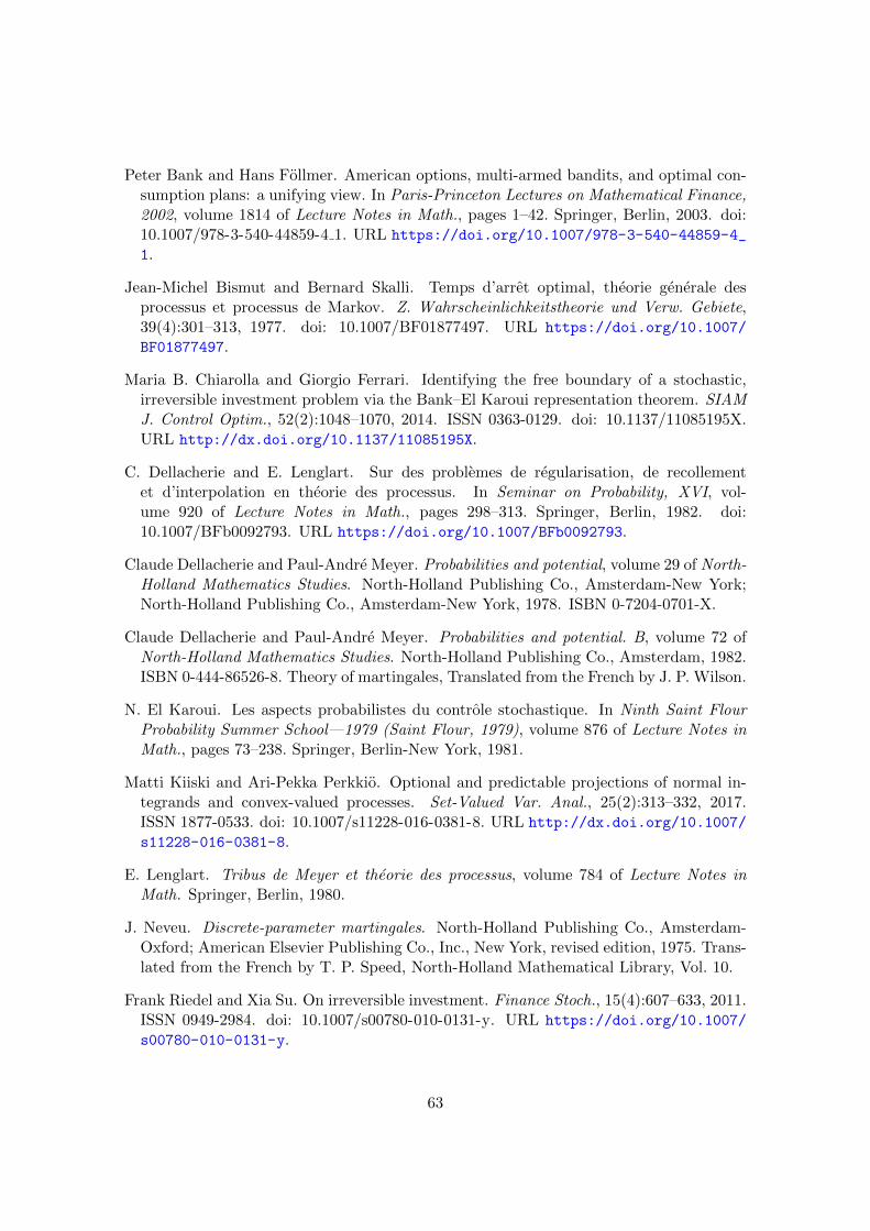
Peter Bank and Hans Follmer. American options, multi-armed bandits, and optimal con-sumption plans: a unifying view. In Paris-Princeton Lectures on Mathematical Finance,2002, volume 1814 of Lecture Notes in Math., pages 1–42. Springer, Berlin, 2003. doi:10.1007/978-3-540-44859-4 1. URL https://doi.org/10.1007/978-3-540-44859-4_

1.

Jean-Michel Bismut and Bernard Skalli. Temps d’arret optimal, theorie generale desprocessus et processus de Markov. Z. Wahrscheinlichkeitstheorie und Verw. Gebiete,39(4):301–313, 1977. doi: 10.1007/BF01877497. URL https://doi.org/10.1007/

BF01877497.

Maria B. Chiarolla and Giorgio Ferrari. Identifying the free boundary of a stochastic,irreversible investment problem via the Bank–El Karoui representation theorem. SIAMJ. Control Optim., 52(2):1048–1070, 2014. ISSN 0363-0129. doi: 10.1137/11085195X.URL http://dx.doi.org/10.1137/11085195X.

C. Dellacherie and E. Lenglart. Sur des problemes de regularisation, de recollementet d’interpolation en theorie des processus. In Seminar on Probability, XVI, vol-ume 920 of Lecture Notes in Math., pages 298–313. Springer, Berlin, 1982. doi:10.1007/BFb0092793. URL https://doi.org/10.1007/BFb0092793.

Claude Dellacherie and Paul-Andre Meyer. Probabilities and potential, volume 29 of North-Holland Mathematics Studies. North-Holland Publishing Co., Amsterdam-New York;North-Holland Publishing Co., Amsterdam-New York, 1978. ISBN 0-7204-0701-X.

Claude Dellacherie and Paul-Andre Meyer. Probabilities and potential. B, volume 72 ofNorth-Holland Mathematics Studies. North-Holland Publishing Co., Amsterdam, 1982.ISBN 0-444-86526-8. Theory of martingales, Translated from the French by J. P. Wilson.

N. El Karoui. Les aspects probabilistes du controle stochastique. In Ninth Saint FlourProbability Summer School—1979 (Saint Flour, 1979), volume 876 of Lecture Notes inMath., pages 73–238. Springer, Berlin-New York, 1981.

Matti Kiiski and Ari-Pekka Perkkio. Optional and predictable projections of normal in-tegrands and convex-valued processes. Set-Valued Var. Anal., 25(2):313–332, 2017.ISSN 1877-0533. doi: 10.1007/s11228-016-0381-8. URL http://dx.doi.org/10.1007/

s11228-016-0381-8.

E. Lenglart. Tribus de Meyer et theorie des processus, volume 784 of Lecture Notes inMath. Springer, Berlin, 1980.

J. Neveu. Discrete-parameter martingales. North-Holland Publishing Co., Amsterdam-Oxford; American Elsevier Publishing Co., Inc., New York, revised edition, 1975. Trans-lated from the French by T. P. Speed, North-Holland Mathematical Library, Vol. 10.

Frank Riedel and Xia Su. On irreversible investment. Finance Stoch., 15(4):607–633, 2011.ISSN 0949-2984. doi: 10.1007/s00780-010-0131-y. URL https://doi.org/10.1007/

s00780-010-0131-y.

63

Walter Rudin. Principles of mathematical analysis. Second edition. McGraw-Hill BookCo., New York, 1964.

64