On a Directionally Adjusted Metropolis-Hastings Algorithm

Mylene Bedard∗ and D.A.S. Fraser†

Abstract

We propose a new Metropolis-Hastings algorithm for sampling from smooth, uni-

modal distributions; a restriction to the method is that the target be optimizable. The

method can be viewed as a mixture of two types of MCMC algorithm; specifically, we

seek to combine the versatility of the random walk Metropolis and the efficiency of

the independence sampler as found with various types of target distribution. This is

achieved through a directional argument that allows us to adjust the thickness of the

tails of the proposal density from one iteration to another. We discuss the relationship

between the acceptance rate of the algorithm and its efficiency. We finally apply the

method to a regression example concerning the cost of construction of nuclear power

plants, and compare its performance to the random walk Metropolis algorithm with

Gaussian proposal.

Keywords: Independence sampler, random walk Metropolis algorithm, Student distribu-

tion, Hessian matrix, Markov chain Monte Carlo

1 Introduction

Metropolis-Hastings algorithms have countless applications in science. They aim to provide

a sample from a distribution of interest, the target distribution, often too complex or high-

dimensional to allow for direct sampling. These efficient sampling methods are particularly∗Departement de mathematiques et de statistique, Universite de Montreal, C.P. 6128, H3C 3J7, Canada.

Allo Email: bedard@dms.umontreal.ca†Department of Statistics, University of Toronto, 100 St. George St., M5S 3G3, Canada. Espaces

alllo Email: dfraser@utstat.toronto.edu.

1

popular in Bayesian statistics, where the distribution of interest in often intractable. In

statistics however, their application is far from limited to the Bayesian framework, and they

can be useful in the classical (or frequentist) approach. In hypothesis testing for instance,

it may be of interest to determine an exact p-value; this may be the case when examining

new or existing methods for computing p-values, or simply when performing a study about

their accuracy (see Bedard et al. 2007).

Common to all Metropolis-Hastings algorithms is the need for selecting a proposal density

q, which is used to propose values to be potentially included in the sample. The character-

istics of the chosen q define the type of algorithm that is used. The most popular class of

Metropolis-Hastings algorithms is undoubtedly that of the random walk Metropolis (RWM)

algorithms. The proposal density of these algorithms is centered around the current value

of the Markov chain (or, in other words, the current value of the sample); standard choices

for the proposal distribution are the normal and the uniform distributions. The proposal

density of a RWM algorithm thus evolves over time, and this results in an algorithm that

is versatile and extremely easy to apply. In fact, practitioners need to make very few ad-

justments before using this algorithm; they only need to tune the variance of the proposal

distribution in the case of a normal proposal, or its range in the case of a uniform pro-

posal. There already exist guidelines in the literature to facilitate this step (Roberts et al.

1997; Roberts and Rosenthal 2001; Bedard 2006 and 2007). As a drawback to the wide

applicability of RWM algorithms, we notice however that their convergence may be lengthy.

This should not come as a surprise when taking into account the versatility of the sampling

method, which may be applied to sample from virtually any target distribution.

A second class of Metropolis-Hastings algorithms contains the independence samplers. For

this class of algorithm, the proposal density q is independent of the previous values in the

Markov chain. From one iteration to another, the proposal density thus remains the same.

When applying MCMC methods, the selection of the proposal distribution always involves

a compromise: the closer it is to the target distribution, the more difficult it is to generate

moves from the proposal distribution but the more efficient is the sampling method. Under

this scheme, we have the opportunity to select a proposal distribution which is close to the

2

target distribution in a certain sense. Hence, the independence sampler has the potential

of enjoying better convergence properties than the RWM algorithm, but it necessitates a

better understanding of the target distribution. Generally, independence samplers are more

problem-specific than RWM algorithms, but they also require more work in order to come

up with a well-suited proposal density.

In this paper, we introduce a new sampling algorithm that could be classified between RWM

algorithms and independence samplers. In other words, we attempt to combine the versa-

tility of the RWM algorithm and the performance of the independence sampler to obtain

samples from smooth and unimodal target densities. As is the case for the independence

sampler, the location of the new proposal distribution is fixed over time; the tails of the

proposal distribution however are fine tuned by what we call a directional adjustment. This

feature ensures that the tails of the target distribution are not neglected; this is an impor-

tant detail, particularly when the estimation of tail probabilities is of interest as was the

case in Bedard et al. (2007).

The idea of selecting the directions in which to sample before proposing an actual sample

value has been addressed by other researchers in the MCMC community. Gilks et al. (1994)

describe the adaptive direction sampling, a generalization of the Gibbs algorithm which

consists in updating one coordinate at a time, but in directions that might not be parallel

to the coordinate axes. The radial-based Metropolis-Hastings algorithm of Bauwens et al.

(2004) features a reparameterization into direction and departure that is similar to that

discussed in the present paper. This algorithm however relies on sampling from the exact

target distribution in various directions, which makes the method time-consuming and more

hassle to implement. As far as general sampling methods are concerned, the importance

sampling technique of Geweke (1989) features a fine tuning of the tails of the importance

sampling density that bears some similarities with the fine tuning we propose for the proposal

distribution. His approach consists in adjusting, for every coordinate, the scaling of the

importance sampling density to match that of the target density; by opposition we use a

Student proposal density as discussed in Brazzale (2000), and adjust its tails by varying the

degrees of freedom. More importantly, we do not restrict to directions that are parallel to

3

the coordinate axes, but we apply this adjustment to every possible direction.

The paper is arranged as follows. In Section 2, we introduce some notation and describe

the type of target distribution for which the new algorithm is designed. In Section 3,

we develop the theory behind the directionally adjusted argument, and in Section 4 we

summarize the necessary steps for implementing the algorithm. To illustrate its application

and its performance, we consider 3- and 8-parameter regression examples in Sections 5 and

6, and compare the new method to both the independence sampler and the RWM algorithm.

We conclude the paper with a discussion in Section 7.

Compared to the RWM algorithm, the resulting algorithm reduces significantly the variances

of estimates; it also produces a high acceptance rate. The acceptance rate of an algorithm

is defined as the proportion of proposed moves that are accepted as suitable values for the

sample. In the case of RWM algorithms, a high acceptance rate is by no mean an indicator

of efficiency for the algorithm; on the contrary it generally is a sign that the algorithm is

exploring the state space too slowly and thus performing sub-efficiently. In the case of an

independence sampler, we are not aware of any theoretical result stating that efficiency is

implied by, or somehow related to a high acceptance rate. Mengersen and Tweedie (1996)

do provide a bound on the ratio of the proposal to the target density that ensures uniform

ergodicity of the algorithm. Although this bound can be related to the transition density of

the algorithm, it does not allow one to draw any conclusion about the acceptance rate itself.

For instance, an independence sampler with a high acceptance rate might indicate that we

sample too much from regions with high target density, and consequently that the proposal

distribution is poorly suited to the problem at hand. Intuitively however, we can deduce

that a high acceptance rate is a favorable attribute in our case. Indeed, if we are positive

that we are not undersampling the tails of the target density, then a high acceptance rate

indicates that we are not wasting energy in proposing too great a number of unsuitable

values for the target; in other words, the proposal is a good fit!

4

2 Some Notation

Consider an n-dimensional target density π (x), x = (x1, . . . , xn). Suppose that we are

interested in obtaining a sample from this density of interest, but that unfortunately there

is no simple way to achieve this directly. We might then use the very general Metropolis-

Hastings algorithm (Metropolis et al. 1953; Hastings 1970), which is implemented through

the following procedure.

Given that the current sample value is xj , we propose a new value for the sample by

generating a value yj+1 from a preferred proposal distribution with density q (yj+1 |xj ).

Then, we accept this proposed value as the new sample value (i.e. we set xj+1 = yj+1) with

probability α (xj ,yj+1), where

α (xj ,yj+1) = 1 ∧ π (yj+1) q (xj |yj+1 )π (xj) q (yj+1 |xj )

; (1)

otherwise, we repeat the current value in the sample and set xj+1 = xj . If we then repeat

this N − 1 times from an initial x0 we will obtain a nominal sample of size N .

This sampling method is very general and might exhibit peformances that are dramatically

different depending on which type of proposal density is selected. As mentioned previously,

one approach is to use the extremely popular RWM algorithm. Usually, the RWM algorithm

employs a proposal density with independent components:

q (yj+1 |xj ) =n∏i=1

qi (yj+1,i |xj ) ,

where qi (yj+1,i |xj ) is the density for the ith component of yj+1. For instance, one might

set Yj+1 ∼ N(xj , σ2In

)for some σ > 0, with In the n-dimensional identity matrix. The

center of the proposal distribution is thus spanning the state space over time. This is a con-

venient practice, but as soon as we are dealing with a multi-dimensional target distribution

which does not possess independent components, as is usually the case, this independence

assumption between the proposal components becomes suboptimal.

Nonetheless, applying the method does not require a very thorough study of the target

density, and may not be much hassle to implement. If we are lucky, we might even benefit

from a reasonable convergence rate to the stationary distribution. However in particular

5

situations, where the density of interest is heavy-tailed for instance, the RWM algorithm may

take more time to explore the space and may exhibit a slower convergence to stationarity,

which may be frequent in the asymptotic context (as n→∞).

Now in the case where the target density π is smooth and unimodal and if we are able

to maximize the density function, then we may be able to take advantage of this extra

information to come up with a refined proposal distribution. In fact, the initial idea would

be to design a proposal density that mimics the target density at its maximum. In other

words, we would like our proposal density not only to have the same mode as the target

density, but also similar curvature properties at the maximum.

For this, let x = arg supx π (x) be the point at which the target density attains its maximum

(the mode), and let π (x) be the value of the density at that maximum. Recall that the

Hessian matrix of the target density is defined as

∂2π∂x2

1

∂2π∂x1∂x2

· · · ∂2π∂x1∂xn

∂2π∂x2∂x1

∂2π∂x2

2· · · ∂2π

∂x2∂xn

......

. . ....

∂2π∂xn∂x1

∂2π∂xn∂x2

· · · ∂2π∂x2

n

, (2)

and will typically be negative definite when evaluated at the mode x; accordingly we take

H = −∂2 log π (x) /∂x∂xT |x=x to be the negative Hessian of the log-density at the maxi-

mum x.

A natural choice for a proposal distribution would then be to select a normal density,

whose location and scaling are adjusted to match x and H−1 respectively. This, however,

illustrates well the problem at hand: the resulting proposal distribution is one that is static,

i.e. whose location does not vary through time, but whose maximum does mimic that of the

target distribution. Using a proposal distribution whose location is static calls for a certain

level of caution, mainly to ensure that we are not undersampling from certain areas of the

state space. Indeed, it is well-known that the normal density has short tails. It is therefore

reasonable to wonder what would happen if we aimed at sampling from a target distribution

with long tails? Since the normal distribution seldom proposes moves located far out in the

tails, we might expect to either neglect the tails of the target distribution, or have to run

6

the algorithm for a very long time before it converges to the stationary distribution. In

order to design an efficient proposal distribution whose location is fixed through time, it is

thus necessary to ensure that it has tails that are heavy enough to match those of the target

distribution.

How does the acceptance rate of an algorithm relate to the efficiency of the proposed method?

For the case of RWM algorithms, it is commonly acknowledged that a high proportion of

accepted moves is usually far from guaranteeing any level of perfomance in the algorithm. In

the case of a Gaussian proposal distribution for instance, a high acceptance rate might reveal

that very small steps are taken at every iteration, and consequently that the algorithm ex-

plores its state space inefficiently. In fact, theoretical results prove that for high-dimensional

target distributions, the proportion of accepted moves that yields the fastest convergence

to the stationary distribution is smaller or equal to 25% (Roberts et al. 1997; Bedard 2006,

2007).

In the case of a proposal distribution whose location is fixed, the acceptance rate must be

interpreted differently. Indeed, because the location of the proposal distribution does not

span the state space but rather remains fixed, it is important that it does not neglect any

region where the target density is positive. In the cases we consider, where the location

of both the target and proposal densities are identical, excessively high or low acceptance

rates could be indicators of two different concerns. A high acceptance rate could indicate

that the proposal distribution is concentrated in regions where the target possesses a high

density only, thus ignoring other regions with lower, but positive density; such a proposal

distribution could then wrongly lead us to oversample from some regions. At some opposite,

the tails of the proposal distribution could be considerably heavier than those of the target

distribution and too great a number of improbable values for the target would be proposed;

this would translate into a reduced acceptance rate, and would consequently alter the speed

of convergence of the algorithm.

As long as we are totally sure that the proposal distribution selected does not neglect any

region of the state space, a high acceptance rate is then an indicator that the proposal is a

good fit for the target considered. Although this is quite intuitive, we are not aware of any

7

general theoretical result confirming this as yet. This might be related to the fact that for a

general form of the target density, it is not straight-forward to design a well-suited proposal

distribution with a fixed location that would allow to observe such an implication. In the

following section, we introduce a directionally adjusted proposal distribution that attempts

to resolve this issue.

3 A Directionally Adjusted Proposal Distribution

3.1 Centering and Scaling the Student Distribution

We aim at sampling efficiently from a smooth and unimodal n-dimensional target density

π. Under this setting, the regions most likely to be neglected using a proposal density that

is centered around x and scaled according to H−1 are the tails of the target density. As

mentioned in the previous section, a normal proposal would not be a wise choice due to

its short tails. To overcome this problem, we consider a distribution with heavier tails, the

n-dimensional Student density with f degrees of freedom; in its canonical form, designated

Studentf (0, In), this density satisfies

qf (t) =Γ(f+n

2

)πn/2Γ

(f2

) (1 + t21 + . . .+ t2n

)− f+n2

=Γ(f+n

2

)πn/2Γ

(f2

) (1 + t′t)− f+n

2 , (3)

where t′ = (t1, . . . , tn). Samples from this distribution are easily generated from any statis-

tical package. Indeed, an observation from an n-dimensional canonical Student distribution

with f degrees of freedom can be obtained as

t′ =

(z1χf, . . . ,

znχf

), (4)

where z1, . . . , zn are independent observations from a standard normal distribution and χ2f

is an observation from a chi-square distribution with f degrees of freedom.

The negative Hessian of the log density at t = 0 for the n-dimensional canonical Student (3)

is equal to (f + n) In. Adjusting the location and scaling to match the location and Hessian

8

of the target density at its mode, the proposal then becomes a Studentf(x, (f + n) H−1

).

For this we then relocate and rescale the generated t’s to obtain

y = x + (f + n)1/2 H−1/2t, (5)

where H1/2 is a right square root matrix of H = (H1/2)′(H1/2), or alternatively we might

use the relation

y = x + w/χf ,

where w designates an observation from a multivariate normal MN(0, (f + n) H−1

).

The general form of the relocated and rescaled proposal density is given as

qf (y) =Γ(f+n

2

)πn/2Γ

(f2

) (1 +(y − x)′ H (y − x)

f + n

)− f+n2

∣∣∣H1/2∣∣∣

(f + n)n/2. (6)

Now all that is left is choosing the degrees of freedom f of the distribution. What value

of f would produce the optimal speed of convergence for the algorithm? On the one hand,

the parameter f has to be small enough to yield tails that are at least as heavy as those

of the target density; on the other hand, a too-small value for f could yield unnecessarily

heavy tails that would slow down the convergence of the algorithm. Furthermore, we have

not yet considered the fact that the picture might vary as we study different directions with

the target density; indeed, the target densities considered are often far from spherically

symmetrical and the behavior of the tails can vary widely over the state space.

Because of the generality of the target densities studied, a natural decision for the degrees

of freedom f of the proposal distribution would be to allow it to vary over time as opposed

to choosing a value fixed for the duration of the algorithm. We find this approach to be

more efficient, particularly for target densities departing from the spherical assumption.

3.2 Expressing Sample Values in Terms of Direction and Departure

The choice of f will then be redetermined at each iteration of the algorithm. For this, we

favor an approach that allows us to match as closely as possible the target and proposal

distributions, while ensuring that the tails of the target are not neglected. The idea we

9

propose for selecting the degrees of freedom f in any given iteration is based on the following

decomposition, and is outlined in Section 3.3.

The discussion is easier if x = 0, the Hessian H = In is the identity, and thus the root

H1/2 = In; accordingly we assume this here and address the more general case later. Looking

from the maximum of the target density, we examine the target π in the direction of the

current state. Suppose that the current state of the algorithm is xj ; we refer to uj = xj/ |xj |

as the direction of xj , where |x| =√x2

1 + . . .+ x2n is the norm of the vector x. The

directional argument uj is approximately uniformly distributed on a unit sphere in Rn; its

density, π (uj), can then be approximated by π (u) ≈ 1/An, where An = 2πn/2/Γ (n/2)

is the surface area of the sphere. Furthermore a random uniform value u can easily be

generated by taking z1, . . . , zn from a unit normal and then standardizing

u′ =(z1, . . . , zn)|z|

. (7)

According to this method, every sample point can then be expressed as xj = uj · sj ; uj is

itself an n-dimensional vector indicating the direction of the current sample point xj from

the mode of the target density, while sj = |xj | gives the radial departure of this sample

point from the mode. Analogously, the target density can be reexpressed in terms of the

directional and departure variables as π (uj , sj) = π (sj |uj ) π (uj).

Using this information and continuing with the assumption that x = 0 and H = In, we

would like to sample from some proposal density q that is as similar as possible to π; although

we chose a Student proposal, we momentarily generalize this choice in the following way.

A proposed yj+1 can be decomposed in a similar manner into its own directional and

departure arguments: yj+1 = upropj+1 · spropj+1 . We can then reexpress the proposal density

q (yj+1) accordingly as

q(upropj+1 , s

propj+1

)= q

(spropj+1

∣∣∣upropj+1

)q(upropj+1

).

Here we now take the marginal uniform density approximation of π (u) as an appropriate

sampling process for the proposed direction, upropj+1 . In other words, it suffices to generate

the proposed direction from (7). To have maximum agreement between the target and

10

proposal densities, we then choose q(spropj+1

∣∣∣upropj+1

)as being an accessible approximation to

the conditional target π (sj |uj ).

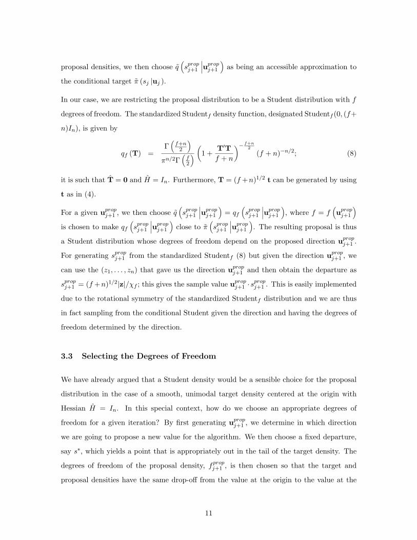
In our case, we are restricting the proposal distribution to be a Student distribution with f

degrees of freedom. The standardized Studentf density function, designated Studentf (0, (f+

n)In), is given by

qf (T) =Γ(f+n

2

)πn/2Γ

(f2

) (1 +T′Tf + n

)− f+n2

(f + n)−n/2; (8)

it is such that T = 0 and H = In. Furthermore, T = (f +n)1/2 t can be generated by using

t as in (4).

For a given upropj+1 , we then choose q(spropj+1

∣∣∣upropj+1

)= qf

(spropj+1

∣∣∣upropj+1

), where f = f

(upropj+1

)is chosen to make qf

(spropj+1

∣∣∣upropj+1

)close to π

(spropj+1

∣∣∣upropj+1

). The resulting proposal is thus

a Student distribution whose degrees of freedom depend on the proposed direction upropj+1 .

For generating spropj+1 from the standardized Studentf (8) but given the direction upropj+1 , we

can use the (z1, . . . , zn) that gave us the direction upropj+1 and then obtain the departure as

spropj+1 = (f +n)1/2|z|/χf ; this gives the sample value upropj+1 ·spropj+1 . This is easily implemented

due to the rotational symmetry of the standardized Studentf distribution and we are thus

in fact sampling from the conditional Student given the direction and having the degrees of

freedom determined by the direction.

3.3 Selecting the Degrees of Freedom

We have already argued that a Student density would be a sensible choice for the proposal

distribution in the case of a smooth, unimodal target density centered at the origin with

Hessian H = In. In this special context, how do we choose an appropriate degrees of

freedom for a given iteration? By first generating upropj+1 , we determine in which direction

we are going to propose a new value for the algorithm. We then choose a fixed departure,

say s∗, which yields a point that is appropriately out in the tail of the target density. The

degrees of freedom of the proposal density, fpropj+1 , is then chosen so that the target and

proposal densities have the same drop-off from the value at the origin to the value at the

11

point upropj+1 · s∗; this reasonably results in good agreement for the tails of the two densities

in the direction upropj+1 .

After having determined the degrees of freedom f for a given iteration, we then generate a

proposed departure spropj+1 by first generating a χf to use in (4) together with the (z1, . . . , zn)

that generated the upropj+1 , as mentioned in the previous section. In effect we are using a

conditional Student distribution special to the direction in order to mimic the target in

that direction as much as possible. The proposed value is thus upropj+1 · spropj+1 , which is then

accepted or rejected according to the usual acceptance function for the Metropolis-Hastings

algorithm.

This procedure results in a proposal density that reproduces the behavior of the target

at the maximum and accomodates the form of the tails. At each iteration, the proposal

is chosen to match the tail in that generated direction of interest. The choice of fpropj+1

for the simplistic case of a one-dimensional target density is illustrated in Figure 1. The

target density represented in this figure (solid curve) possesses a relatively heavy tail on

the right hand side, and a light tail on the left hand side. When sampling in a direction

pointing to the right for such a target density, we propose the Student distribution (dashed

curve) with a heavier tail (i.e., smaller degrees of freedom) than if we were sampling in the

opposite direction. From the graph, we also notice the point at which the proposal and

target densities intersect; for this the target has been rescaled vertically so the drop-off is

from a common maximum.

Finding the degrees of freedom fpropj+1 for a given iteration involves solving the equation

π(upropj+1 · s∗

)π (0)

=qfprop

j+1

(upropj+1 · s∗

)qfprop

j+1(0)

=

1 +

(upropj+1 · s∗

)′ (upropj+1 · s∗

)fpropj+1 + n

−

fpropj+1

+n

2

, (9)

where upropj+1 is the generated direction for a new value, and s∗ is the distance from the mode

to the point where we want the proposal and target densities to intersect in the direction

upropj+1 .

12

Figure 1: Graph of the target (solid) and proposal (dashed) densities when proposing a

value in the direction pointing to the right of the graph. The intersection point is upropj+1 · s∗.

−2 0 2 4

0.00.2

0.40.6

0.81.0

●

There does not exist a closed-form solution for fpropj+1 in the previous equation. In practice,

it is not necessary to solve for the exact value of fpropj+1 in (9); for pragmatic reasons, we

restrict fpropj+1 to be an integer value between 1 (Cauchy distribution) and 50 (near normal

distribution). If we let r2 = 2 log{π (0) /π

(upropj+1 · s∗

)}be the target likelihood ratio quan-

tity and let Q2 =(upropj+1 · s∗

)′ (upropj+1 · s∗

)be the quadratic departure for the standardized

Student, we can solve for fpropj+1 + n = f using

f log

(1 +

Q2

f

)= r2. (10)

This can be achieved by scanning the values for fpropj+1 in {1, 2, . . . , 50} and choosing the

closest fit.

3.4 Choosing s∗

There remains one issue to be discussed before being ready to implement the outlined

method. We mentioned that we choose the degrees of freedom of the proposal distribution

at every iteration so that both the target and proposal densities intersect at an appropriate

13

point in the tail in the given direction. How do we choose s∗, the departure from the mode

at which we would like to force an agreement between the target and proposal densities?

To address this issue we once again focus on the standardized version of the target density

where we have x = 0 and H = In; it should be emphasized that this adjustment does not

limit the proposed method as we shall see in Section 4. If the target happened to correspond

to the case where the coordinates are independent and approximately normal, then we would

have Y ∼ N(0, In) and the distribution of (spropj+1 )2 = |yj+1|2 given upropj+1 = yj+1/ |yj+1|

would be a chi square with n degrees of freedom. Consequently, the conditional distribution

for departure of the proposed value given its direction, spropj+1 |upropj+1 , would simply be chi in

distribution with n degrees of freedom; an approximate mean value for this is√n. We thus

suggest forcing the target and proposal densities to intersect at a departure of s∗ = λ√n

from the mode, where λ is a tuning parameter. From our experience, λ can be chosen to

be 2 or 3 for instance; when chosen in this range, the exact value of the tuning parameter

usually has an insignificant impact on the performance of the algorithm.

Accordingly we examine the target distribution drop off at such a distance in the chosen

direction and use a degrees of freedom f that boosts the tails of the proposal distribution

to match those of the target. We thus choose f to give π(s∗|upropj+1

)/qf

(s∗|upropj+1

)to the

degree possible with f in a sensible range of 1, . . . , 50.

The resulting proposal density is thus one that has the same location and the same cur-

vature at the maximum as the target density but that also replicates the tail thickness in

the direction of the proposed sample value. The Metropolis-Hastings algorithm can then be

carried through as usual, by proposing a value from a multivariate Student with the desig-

nated degrees of freedom, and then accepting or rejecting this proposed value according to

the usual acceptance probability. Overall this results in an algorithm whose proposal has

central form that stays fixed throughout time, but whose tails becomes thicker or lighter

from one iteration to another depending on the direction from the center of the distribution.

We do note a small technical point concerning the overall effective proposal density. We

have spoken of having a particular curvature and Hessian at the maximum. By varying the

degrees of freedom with direction we will have differing heights coming to the maximum

14

from differing directions and indeed have a discontinuity at the maximum; this is of no

practical significance.

4 The Algorithm

The sampling algorithm introduced herein is valid for general target densities π. To im-

plement the method, it is however convenient to work with a standardized version of the

target density. Specifically, we consider x∗ = H1/2 (x− x), where H1/2 is a right square

root matrix of H such that H = (H1/2)′(H1/2

). This can easily be obtained with the

functions pdMat and pdFactor, located in the package nlme of the statistical freeware R.

This adjustment implies that x∗ = 0 and H∗ = In. The standardized target density satisfies

π∗ (x∗) = π(x + H−1/2x∗

) ∣∣∣H−1/2∣∣∣ ∝ π (x + H−1/2x∗

)= π (x) ,

where H−1/2 is the inverse of H1/2 and∣∣∣H−1/2

∣∣∣ is the determinant of the former; we can

thus access standardized density at x∗ by using the original π with the x value obtained

from the mapping x = x + H−1/2x∗.

We also assume that determinations of x and H are available; in the statistical freeware

R for instance, x can usually be obtained with the function nlm. The Hessian can either

be computed directly using the second derivatives of the density, or obtained numerically

with the function fdHess. For the algorithm we assume that this standardization has been

applied and is used for the following.

Given that xj is the time-j state of the algorithm, we perform the following two preliminary

steps if not available from preceding calculations:

a. Determine the direction of the standardized current sample value x∗j = H1/2(xj − x):

uj = x∗j/∣∣∣x∗j ∣∣∣.

b. Choose the integer value among {1, 2, . . . , 50} which is closest to the solution to (10)

for uj ; call it fj .

Once these steps are executed, we are ready to iterate:

15

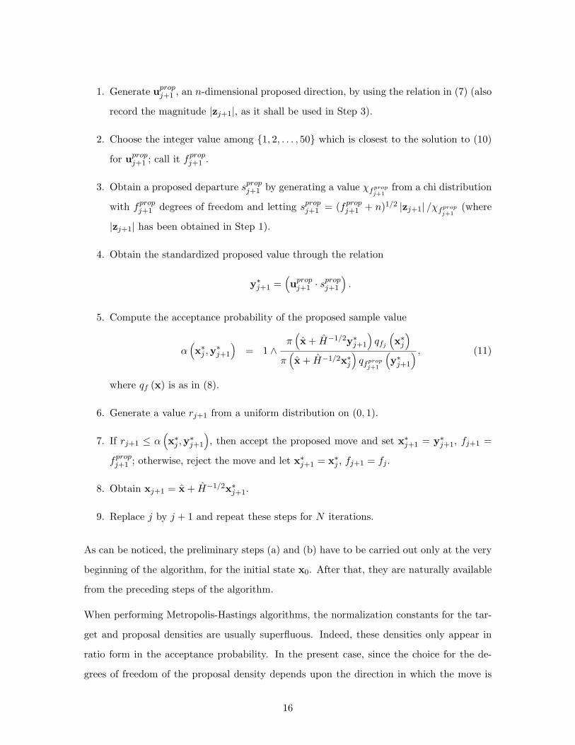
1. Generate upropj+1 , an n-dimensional proposed direction, by using the relation in (7) (also

record the magnitude |zj+1|, as it shall be used in Step 3).

2. Choose the integer value among {1, 2, . . . , 50} which is closest to the solution to (10)

for upropj+1 ; call it fpropj+1 .

3. Obtain a proposed departure spropj+1 by generating a value χfpropj+1

from a chi distribution

with fpropj+1 degrees of freedom and letting spropj+1 = (fpropj+1 + n)1/2 |zj+1| /χfpropj+1

(where

|zj+1| has been obtained in Step 1).

4. Obtain the standardized proposed value through the relation

y∗j+1 =(upropj+1 · s

propj+1

).

5. Compute the acceptance probability of the proposed sample value

α(x∗j ,y

∗j+1

)= 1 ∧

π(x + H−1/2y∗j+1

)qfj

(x∗j)

π(x + H−1/2x∗j

)qfprop

j+1

(y∗j+1

) , (11)

where qf (x) is as in (8).

6. Generate a value rj+1 from a uniform distribution on (0, 1).

7. If rj+1 ≤ α(x∗j ,y

∗j+1

), then accept the proposed move and set x∗j+1 = y∗j+1, fj+1 =

fpropj+1 ; otherwise, reject the move and let x∗j+1 = x∗j , fj+1 = fj .

8. Obtain xj+1 = x + H−1/2x∗j+1.

9. Replace j by j + 1 and repeat these steps for N iterations.

As can be noticed, the preliminary steps (a) and (b) have to be carried out only at the very

beginning of the algorithm, for the initial state x0. After that, they are naturally available

from the preceding steps of the algorithm.

When performing Metropolis-Hastings algorithms, the normalization constants for the tar-

get and proposal densities are usually superfluous. Indeed, these densities only appear in

ratio form in the acceptance probability. In the present case, since the choice for the de-

grees of freedom of the proposal density depends upon the direction in which the move is

16

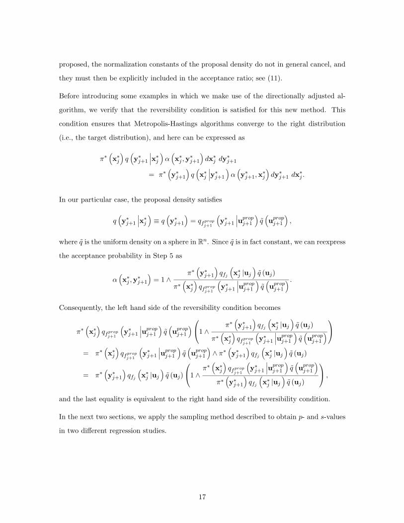
proposed, the normalization constants of the proposal density do not in general cancel, and

they must then be explicitly included in the acceptance ratio; see (11).

Before introducing some examples in which we make use of the directionally adjusted al-

gorithm, we verify that the reversibility condition is satisfied for this new method. This

condition ensures that Metropolis-Hastings algorithms converge to the right distribution

(i.e., the target distribution), and here can be expressed as

π∗(x∗j)q(y∗j+1

∣∣∣x∗j )α (x∗j ,y∗j+1

)dx∗j dy

∗j+1

= π∗(y∗j+1

)q(x∗j∣∣∣y∗j+1

)α(y∗j+1,x

∗j

)dy∗j+1 dx

∗j .

In our particular case, the proposal density satisfies

q(y∗j+1

∣∣∣x∗j ) ≡ q (y∗j+1

)= qfprop

j+1

(y∗j+1

∣∣∣upropj+1

)q(upropj+1

),

where q is the uniform density on a sphere in Rn. Since q is in fact constant, we can reexpress

the acceptance probability in Step 5 as

α(x∗j ,y

∗j+1

)= 1 ∧

π∗(y∗j+1

)qfj

(x∗j |uj

)q (uj)

π∗(x∗j)qfprop

j+1

(y∗j+1

∣∣∣upropj+1

)q(upropj+1

) .Consequently, the left hand side of the reversibility condition becomes

π∗(x∗j)qfprop

j+1

(y∗j+1

∣∣∣upropj+1

)q(upropj+1

)1 ∧π∗(y∗j+1

)qfj

(x∗j |uj

)q (uj)

π∗(x∗j)qfprop

j+1

(y∗j+1

∣∣∣upropj+1

)q(upropj+1

)

= π∗(x∗j)qfprop

j+1

(y∗j+1

∣∣∣upropj+1

)q(upropj+1

)∧ π∗

(y∗j+1

)qfj

(x∗j |uj

)q (uj)

= π∗(y∗j+1

)qfj

(x∗j |uj

)q (uj)

1 ∧π∗(x∗j)qfprop

j+1

(y∗j+1

∣∣∣upropj+1

)q(upropj+1

)π∗(y∗j+1

)qfj

(x∗j |uj

)q (uj)

,and the last equality is equivalent to the right hand side of the reversibility condition.

In the next two sections, we apply the sampling method described to obtain p- and s-values

in two different regression studies.

17

5 Toy Example

5.1 Background

As a first example of the applicability and efficiency of the method, we shall focus on the

regression example discussed in Bedard et al. (2007). Specifically we consider the following

data, which has been generated from the null linear regression model yi = α + βxi + σzi

with α = 0, β = 1, σ = 1, and k = 7:

xi -3 -2 -1 0 1 2 3

yi -2.68 -4.02 -2.91 0.22 0.38 -0.28 0.03

The response variability is the Student density with 7 degrees of freedom (no connection

with k = 7) and thus the density of the response can be expressed as

f (y;α, β, σ) dy = σ−77∏i=1

h

(yi − α− xiβ

σ

)dyi,

where h (z) is the Student density with 7 degrees of freedom.

Let us suppose that we are interested in testing the hypothesis β = 1. This can be achieved

from the Bayesian and the classical perspectives, by respectively computing the posterior

survivor value (s-value) and the p-value. We shall examine the performance of the direc-

tionally adjusted algorithm under both approaches. This type of example is particularly

appealing in the present context; indeed, it is interesting to see how the method performs

for the evaluation of tail probabilities.

In the Bayesian setting, we select the default prior dα dβ d log σ to perform the analysis; this

choice of prior distribution yields s- and p-values that are equivalent under both frameworks,

as discussed in Bedard et al. (2007). The default prior selected points towards a more natural

choice for the parameter of interest; we shall then use (α, β, log σ) rather than (α, β, σ), a

convenient parameterization which also has the advantage of avoiding boundary problems.

The posterior distribution of (α, β, log σ) is then

π1

(α, β, τ

∣∣∣y0)dα dβ dτ = c e−7τ

7∏i=1

{1 +

(y0i − α− βxi)2

7e2τ

}−4

dα dβ dτ. (12)

18

To obtain the exact s-value for testing the hypothesis that β is equal to 1, it suffices to

obtain a sample from this posterior density and to record the number of values of β located

to the right of the value of interest:

s(β) =1N

N∑j=1

I (βj ≥ β) =1N

N∑j=1

I (βj ≥ 1) , (13)

where N is the size of the sample generated.

The approach for obtaining the exact p-value under the classical approach is discussed in

details in Section 6, which considers a similar model. For now, we shall just mention that a

sample needs to be obtained from a reparameterized density of interest

π2

(a, b, g

∣∣∣d0)da db dg = c e5g

7∏i=1

(1 +

(a+ bxi + egd0i )

2

7

)−4

da db dg, (14)

where d0i = (y0

i − xib0)/eg0 and b0, g0 are the least-squares estimates from the data. The

p-value can then be computed by using

p(β) =1N

N∑j=1

I

(bjegj

<b0 − βeg0

)=

1N

N∑j=1

I

(bjegj

<b0 − 1eg0

). (15)

5.2 Simulations

We compare s- and p-values obtained when applying three different types of Metropolis-

Hastings algorithms. In particular, we sample from the target densities π1 in (12) and π2

in (14) by using a random walk Metropolis algorithm with a normal proposal, an indepen-

dence sampler with a Student7(x, (f + n)H−1) proposal distribution, and the directionally

adjusted algorithm described previously. We choose a proposal variance of 0.16 for the

RWM algorithm; this parameter, just like the parameters of the independence proposal,

have been selected so as to yield a reasonable speed of convergence for the algorithms.

In order to estimate the accuracy of the values obtained through each of the methods

considered, we use the following approach. For each combination of algorithm and target

density, we obtain a sample of size N = 4, 000, 000. We split this vector into 4,000 batches

that each contains 1,000 consecutive sample values. In each batch, we drop the first 50

sample values and thus keep the remaining 950 sample values only. We can then compute

19

Table 1: Bayesian s-values and frequentist p-values for testing the hypothesis β = 1 using

three different Metropolis-Hastings algorithms with 4.106 iterations.

Test procedure p-value s-value

RWM - Normal(xj , 0.16) .10821 .10778

(Simulation SD) (.03400) (.03475)

{Acceptance rate} {32.8%} {36.7%}

Independence sampler - Student7(x, (f + n)H−1) .10821 .10761

(Simulation SD) (.03195) (.03355)

{Acceptance rate} {76.0%} {62.7%}

DAMcMC .10773 .10781

(Simulation SD) (.03184) (.03268)

{Acceptance rate} {89.3%} {66.5%}

[Mean fprop] [37.88] [28.57]

the s- or p-values obtained from each batch using (13) or (15) respectively; this yields a vector

containing 4,000 s- or p-values that are approximately independent from each other. The

exact s- or p-value is estimated by recording the sample average of the 4,000 s- or p-values

from the vector. The simulation standard deviation can then be obtained by computing

the sample standard deviation of the vector and dividing this number by√

4, 000; for more

details, we refer the reader to the appendix in Bedard et al. (2007). The numbers obtained

under both the Bayesian and classical frameworks appear in Table 1. We also recorded

the acceptance rate of each of the algorithms, as well as the average value of the proposed

degrees of freedom (∑Nj=1 f

propj+1 /N) for the directionally adjusted algorithm.

The s- and p-values obtained are very similar for each of the three methods studied. It

is interesting to note a significant decrease in the simulation standard deviation of the DA

algorithm when compared to the RWM algorithm; in the Bayesian framework, the simulation

20

standard deviation of the DA algorithm is reduced by a factor of about 1.8 compared to that

of the RWM algorithm while in the classical framework, this factor is close to 2.2. We also

observe that the Bayesian target density π1 possesses longer tails than the frequentist target

density π2. This can be witnessed by checking the mean value of the proposed degrees of

freedom recorded in Table 1.

The DA algorithm also shows some improvement over the independence sampler in terms

of the simulation standard deviation although, as expected, the difference in efficiency is

not as flagrant. Nonetheless, it is generally difficult to be certain of the appropriateness

of the proposal distribution selected for an independence sampler, especially when working

in large dimensions. When applying the DA algorithm, a suitable degrees of freedom is

selected automatically at every iteration; since one needs not fix a conservative degrees of

freedom to ensure a rapid convergence as is the case for the independence sampler, this

results in a gain in efficiency.

It is not appropriate to compare the acceptance rate of the RWM algorithm with the accep-

tance rates of the independence sampler and DA algorithm. Indeed, the acceptance rate of

the RWM algorithm might be tuned through the variance of the normal proposal; here, we

used existing theory on the subject to select a proposal variance that should roughly yield a

chain converging as fast as possible to its stationary distribution. We can however compare

the acceptance rates obtained with the independence sampler and the DA algorithm. We

notice that the acceptance rate of the DA algorithm is consistently and significantly higher

than that obtained with the independence sampler; this intuitively tells us that the proposal

density of the DA algorithm consists in a better fit for both our Bayesian and frequentist

target densities. In particular, the acceptance rate of the DA algorithm for computing the

p-value recorded in Table 1 is surprisingly high, which means that the proposal density is

even better suited for the target density (14) in the classical framework than for (12) in the

Bayesian framework. In general, a large discrepancy between the acceptance rates of the

independence sampler and DA algorithm might reveal an important variation in the tails

behavior in different directions; it might also mean that the independence proposal is much

too conservative.

21

Although longer to run than its competitors, we finally mention that the relative efficiency

gained by using the DA algorithm makes it worth programming. For instance, running the

DA algorithm for this toy example is no longer than about twice the running time of the

RWM algorithm, and this factor decreases as the dimension of the target density increases.

The difference between the running times of the independence sampler considered here

and the DA algorithm are even less important; added to the extra advantages of the DA

algorithm discussed earlier, it is preferable to use the latter.

6 Example

6.1 Background

We consider a dataset concerning the cost of construction of nuclear power plants (Example

G; Cox and Snell, 1981). Specifically, we have information about 32 light water reactor

(LWR) power plants constructed in the USA. The dataset includes 10 explanatory variables,

in addition to a constant; it can be found in the Appendix, along with the description of

the various explanatory variables.

The chosen response is the natural logarithm of the capital cost (logC), and all the other

quantitative variables have also been taken in log form (logS, log T1, log T2, and logN).

According to the analysis in Cox and Snell (1981) and in Brazzale et al. (2007), a linear

regression model seems suitable for this example. There are 4 explanatory variables that

are dismissed as non significant (log T1, log T2, PR, and BW); see the ANOVA table on page

86 of Cox and Snell (1981). The indicated model thus uses the remaining 7 variables, these

being the constant plus D, logS, NE, CT, logN , and PT. Of particular interest is how the

capital cost C depends on N , the cumulative number of power plants constructed by each

architect-engineer.

Brazzale et al. (2007) first investigated the suitability of a Student distribution with 4

degrees of freedom as the error distribution. The corresponding model is then

y = Xβ + σz,

22

where the design matrix X is the 32 x 7 matrix containing the chosen explanatory variables,

and z is distributed according to a Student distribution with 4 degrees of freedom. The

density of the response is then

f (y;β, σ) dy = σ−nn∏i=1

h

(yi −Xiβ

σ

)dyi,

where h (z) is the Student density with 4 degrees of freedom and Xi is the ith row of the

design matrix.

The observed standardized residuals can be recorded as d0 =(y0 −Xb0

)/s0 where for

convenience we use the least squares regression coefficients b and the related error standard

deviation s satisfying s2 =∑ni=1(yi − yi)2/(n − r) with n = 32 and r = 7. The observed

likelihood function is then

L0 (β, σ) = σ−nn∏i=1

h

(y0i −Xiβ

σ

)

= σ−nn∏i=1

h

(s0d0

i −Xi(β − b0

)σ

).

The residuals d0 have an effect on the precision of the estimates of β and σ when there

is error structure other than the usual normal. This is partly reflected in the observed

likelihood function L0 (β, σ) and would then be available for default Bayesian analysis using

the familiar default prior σ−1 dβ dσ. By contrast with a full model f (y;β, σ) analysis

the available precision is not taken account of. Accordingly we use the conditional model

f(y∣∣d0 ;β, σ

)obtained by conditioning on the identified standardized residuals d0:

f(b, s

∣∣∣d0 ;β, σ)db ds = cσ−n

n∏i=1

h

(sd0i −Xi (β − b)

σ

)sn−r−1db ds,

where n = 32 and n− r − 1 = 24.

Now suppose we are interested in the kth regression coefficient; here k = 6 corresponding

to the explanatory variable logN . The corresponding standardized departure is tk = (bk −

βk)/c1/2kk s where ckk is the (k, k) element of the matrix C = (X ′X)−1; it has observed

value t0k(βk) = (b0k − βk)/c1/2kk s

0 and does of course depend on the value βk being assessed.

Due to invariance properties of the model it suffices to compare t0k with the distribution of

23

tk = bk/c1/2kk s from the null model with β = 0 and σ = 1

f(b, s

∣∣∣d0)db ds = c

n∏i=1

h(sd0i +Xib

)sn−r−1db ds

on the r + 1 dimensional space {b, s}, or with the distribution of tk = bk/c1/2kk e

a from

f(b, a

∣∣∣d0)db da = c

n∏i=1

h(ead0

i +Xib)ea(n−r)db da (16)

on Rr+1; the latter can avoid boundary problems.

We thus wish to sample from the target (16) and evaluate the p-value function p(βk) that

gives the percentage position of the observed data relative to the value βk for the particular

explanatory variable:

p (βk) =# tk (b, s) < t0k (βk)

N; (17)

here N is the size of the simulation and the numerator gives the number of instances (b, s)

yielding a value less than the observed t0k(βk).

6.2 Simulations

We compare p-values for testing β6 = −0.1, β6 = −0.01, and β6 = 0.02; for each of these

hypotheses, the p-values are obtained by applying the three Metropolis-Hastings algorithms

considered in Section 5.2. To obtain an efficient speed of convergence for the RWM algo-

rithm, we however select a proposal variance of 0.0001 (i.e. a proposal standard deviation of

0.01). The approach chosen for carrying the MCMC simulations and obtaining the desired

p-values is the same as that described in that section. Specifically, we generate a sample

of size 4,000,000 that we split into 4,000 batches, each containing 1,000 sample values. We

then drop the first 50 values in each of the batches and compute the p-values from (17) by

using the last 950 values of each batch only. From the resulting vector of 4,000 p-values,

we obtain the sample mean and the simulation standard deviation (sample SD/√

4, 000; see

Bedard et al. 2007) for each of the three sampling methods selected for comparison. Once

again, we record the average acceptance rate of each algorithm, and the average value of

the proposed degrees of freedom for the DA algorithm. The results of the simulations are

24

Table 2: Frequentist p-values for testing the hypotheses β6 = −0.1,−0.01, 0.02 using three

different Metropolis-Hastings algorithms with 4.106 iterations. The frequentist third order

p-values are also included for comparison.

Test procedure β6 = −0.1 β6 = −0.01 β6 = 0.02

Thrid order .75283 .10936 .03646

RWM - Normal(xj , 0.0001) .88263 .09019 .01354

(Simulation SD) (.02399) (.02388) (.02135)

{Acceptance rate} {34.5%} {34.6%} {34.5%}

Independence sampler - Student7(x, (f + r + 1)H−1) .75675 .11679 .03766

(Simulation SD) (.03482) (.03341) (.03185)

{Acceptance rate} {36.9%} {36.9%} {36.9%}

DAMcMC .75712 .11695 .03746

(Simulation SD) (.03328) (.03232) (.03140)

{Acceptance rate} {71.6%} {71.6%} {71.6%}

[Mean fprop] [48.24] [48.24] [48.24]

recorded in Table 2; for each hypothesis, we also included the frequentist third order p-value.

The general relationship between hypotheses and their corresponding p-value for different

sampling methods is depicted in Figure 2.

Contrarily to the toy example of Section 5, the p-values obtained with the three sampling

methods selected are not all very close for a given hypothesis. In this higher-dimensional

setting, the RWM algorithm does not perform well for the task at hand, i.e. the computation

of tail probabilities. In fact, the results obtained under this sampling scheme are very

unstable; this can be witnessed by examining Figure 2, which shows two different runs of

the RWM algorithm (the dashed curves). Although these two runs embrace the p-values

25

Figure 2: Graph of p-values versus hypotheses H0 obtained by using the DA (solid) and

RWM (dashed) algorithms, as well as the third order approximation (symbols).

−0.20 −0.15 −0.10 −0.05 0.00 0.05 0.10

0.0

0.2

0.4

0.6

0.8

1.0

H0

p−va

lue

DA algorithm

RWM algorithm

Third order

26

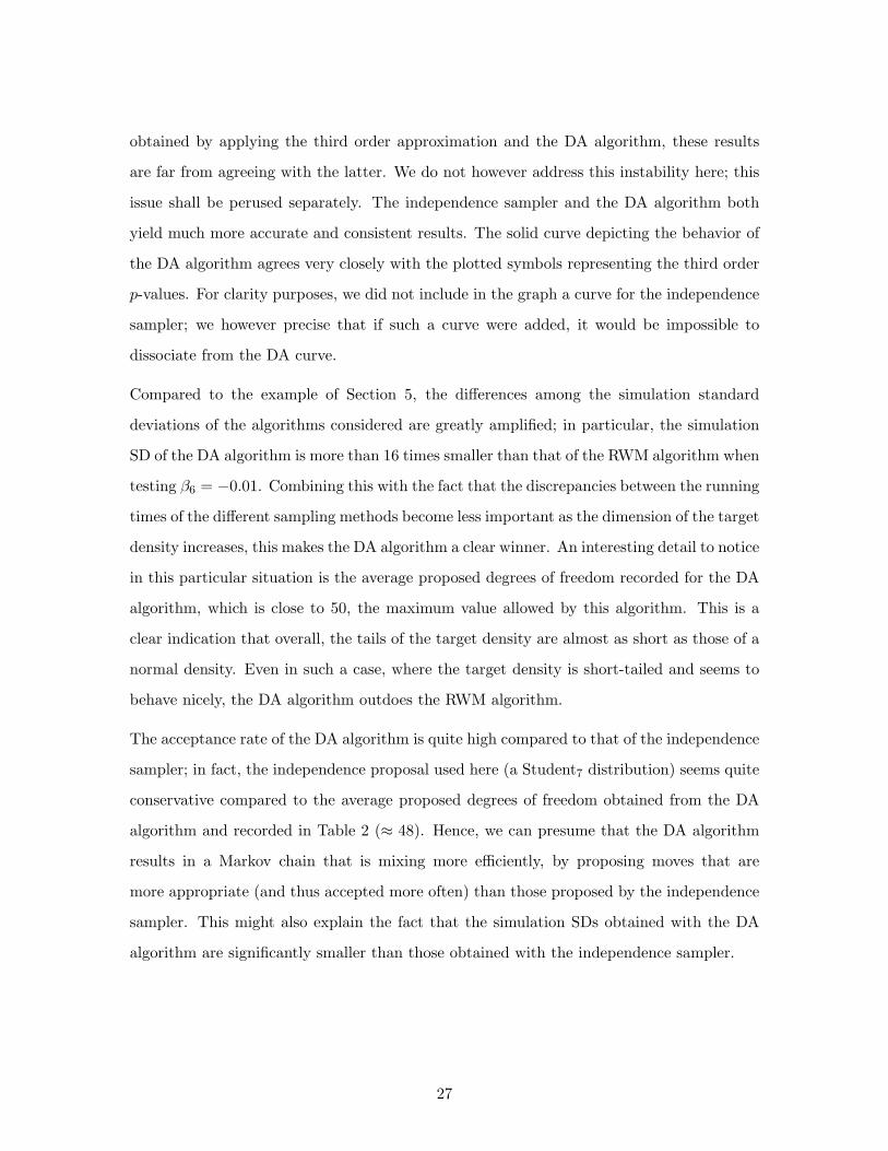
obtained by applying the third order approximation and the DA algorithm, these results

are far from agreeing with the latter. We do not however address this instability here; this

issue shall be perused separately. The independence sampler and the DA algorithm both

yield much more accurate and consistent results. The solid curve depicting the behavior of

the DA algorithm agrees very closely with the plotted symbols representing the third order

p-values. For clarity purposes, we did not include in the graph a curve for the independence

sampler; we however precise that if such a curve were added, it would be impossible to

dissociate from the DA curve.

Compared to the example of Section 5, the differences among the simulation standard

deviations of the algorithms considered are greatly amplified; in particular, the simulation

SD of the DA algorithm is more than 16 times smaller than that of the RWM algorithm when

testing β6 = −0.01. Combining this with the fact that the discrepancies between the running

times of the different sampling methods become less important as the dimension of the target

density increases, this makes the DA algorithm a clear winner. An interesting detail to notice

in this particular situation is the average proposed degrees of freedom recorded for the DA

algorithm, which is close to 50, the maximum value allowed by this algorithm. This is a

clear indication that overall, the tails of the target density are almost as short as those of a

normal density. Even in such a case, where the target density is short-tailed and seems to

behave nicely, the DA algorithm outdoes the RWM algorithm.

The acceptance rate of the DA algorithm is quite high compared to that of the independence

sampler; in fact, the independence proposal used here (a Student7 distribution) seems quite

conservative compared to the average proposed degrees of freedom obtained from the DA

algorithm and recorded in Table 2 (≈ 48). Hence, we can presume that the DA algorithm

results in a Markov chain that is mixing more efficiently, by proposing moves that are

more appropriate (and thus accepted more often) than those proposed by the independence

sampler. This might also explain the fact that the simulation SDs obtained with the DA

algorithm are significantly smaller than those obtained with the independence sampler.

27

7 Discussion

We have introduced a new type of Metropolis-Hastings algorithm for sampling from smooth

and unimodal target densities, the directionally adjusted (DA) algorithm. The idea behind

this method can be divided in two steps: we first use the location and Hessian of the target

density to build a proposal density that reproduces the target behavior at its maximum; we

then let the tail thickness of the proposal be adjusted at every iteration, by an automatic

procedure that attempts to match the tails of the target as closely and efficiently as possible.

We tested this sampling method on two different regression examples; the first example used

simulated data, and the second one real data. Specifically, we evaluated the performance of

the new algorithm by comparing it with the results produced by a RWM algorithm and an

independence sampler. Performance was based on the accuracy of the estimates (p- and s-

values along with their simulation standard deviations), the running times of the algorithms,

as well as the acceptance rate produced by the methods.

In brief we have found that the DA algorithm consistently outperforms its competitors when

looking at the accuracy of the estimates produced. The superiority of the DA algorithm

is even more shocking when working in relatively high-dimensional settings, as the discrep-

ancies between the running times of the RWM algorithm, independence sampler, and DA

algorithm tend to vanish as the dimension of the target density increases. The results from

Section 6 are particularly surprising, as they revealed that traditional sampling methods

can go badly wrong when working in higher dimensions. The comparison of the acceptance

rates obtained also allowed us to conclude that the DA algorithm yields Markov chains that

are mixing more efficiently than those produced by the independence sampler.

8 Appendix

The dataset used in the example of Section 6 appears in Table 3; the description of the

explanatory variables can be found in Table 4.

28

Table 3: Data on 32 LWR power plants in the USA

C D T1 T2 S PR NE CT BW N PT

460.05 68.58 14 46 687 0 1 0 0 14 0

452.99 67.33 10 73 1065 0 0 1 0 1 0

443.22 67.33 10 85 1065 1 0 1 0 1 0

652.32 68.00 11 67 1065 0 1 1 0 12 0

642.23 68.00 11 78 1065 1 1 1 0 12 0

345.39 67.92 13 51 514 0 1 1 0 3 0

272.37 68.17 12 50 822 0 0 0 0 5 0

317.21 68.42 14 59 457 0 0 0 0 1 0

457.12 68.42 15 55 822 1 0 0 0 5 0

690.19 68.33 12 71 792 0 1 1 1 2 0

350.63 68.58 12 64 560 0 0 0 0 3 0

402.59 68.75 13 47 790 0 1 0 0 6 0

412.18 68.42 15 62 530 0 0 1 0 2 0

495.58 68.92 17 52 1050 0 0 0 0 7 0

394.36 68.92 13 65 850 0 0 0 1 16 0

423.32 68.42 11 67 778 0 0 0 0 3 0

712.27 69.50 18 60 845 0 1 0 0 17 0

289.66 68.42 15 76 530 1 0 1 0 2 0

881.24 69.17 15 67 1090 0 0 0 0 1 0

490.88 68.92 16 59 1050 1 0 0 0 8 0

567.79 68.75 11 70 913 0 0 1 1 15 0

665.99 70.92 22 57 828 1 1 0 0 20 0

621.45 69.67 16 59 786 0 0 1 0 18 0

608.80 70.08 19 58 821 1 0 0 0 3 0

473.64 70.42 19 44 538 0 0 1 0 19 0

697.14 71.08 20 57 1130 0 0 1 0 21 0

207.51 67.25 13 63 745 0 0 0 0 8 1

288.48 67.17 9 48 821 0 0 1 0 7 1

284.88 67.83 12 63 886 0 0 0 1 11 1

280.36 67.83 12 71 886 1 0 0 1 11 1

217.38 67.25 13 72 745 1 0 0 0 8 1

270.71 67.83 7 80 886 1 0 0 1 11 1

29

Table 4: Notation for data in Table 3

C Cost in dollars ×10−6, adjusted to 1976 base

D Date construction permit issued

T1 Time between application for and issue of permit

T2 Time between issue of operating licence and construction permit

S Power plant net capacity (MWe)

PR Prior existence of an LWR on same site (= 1)

NE Plant constructed in north-east region of USA (= 1)

CT Use of cooling tower (= 1)

BW Nuclear steam supply system manufactured by Babcock-Wilcox (= 1)

N Cumulative number of power plants constructed by each architect-engineer

PT Partial turnkey plant (= 1)

References

Bauwens, L., Bos, C. S., van Dijk, H. K., and van Oest, R. D. (2004) Adaptive radial-

based direction sampling: some flexible and robust Monte Carlo integration methods. J.

Econometrics, 123, 201-25.

Bedard, M. (2007) Weak convergence of Metropolis algorithms for non-iid target distribu-

tions. Ann. Appl. Probab., 17, 1222-44.

Bedard, M. (2006) Optimal acceptance rates for Metropolis algorithms: Moving beyond

0.234. To appear in Stochastic Process. Appl.

Bedard, M., Fraser, D. A. S., and Wong, A. (2007) Higher accuracy for Bayesian and

frequentist inference: Large sample theory for small sample likelihood. Statist. Sci., 22,

301-21.

Brazzale, A. R. (2000) Practical Small Sample Parametric Inference. Ph.D. thesis, Ecole

Polytechnique Federale de Lausanne.

Brazzale, A. R., Davison, A. C., and Reid, N. (2007) Applied Asymtotics: Case Studies in

Small-Sample Statistics. Cambridge University Press.

30

Cox, D. R., Snell, E. J. (1981) Applied Statistics: Principles and Examples. Chapman and

Hall.

Geweke, J. (1989) Bayesian inference in econometric models using Monte Carlo integration.

Econometrica, 57, 1317-39.

Gilks, W. R., Roberts, G. O., and George, E. I. (1994) Adaptive direction sampling. The

Statistician, 43, 179-89.

Hastings, W. K. (1970) Monte Carlo sampling methods using Markov chains and their

applications. Biometrika, 57, 97-109.

Mengersen, K. L. and Tweedie, R. L. (1996) Rates of convergence of the Hastings and

Metropolis algorithms. Ann. Statist. 24, 101-21.

Metropolis, N., Rosenbluth, A. W., Rosenbluth, M. N., Teller, A. H., and Teller, E. (1953)

Equations of state calculations by fast computing machines. Journal of Chemical Physics,

21, 1087-92.

Roberts, G. O., Gelman, A., and Gilks, W. R. (1997) Weak convergence and optimal scaling

of random walk Metropolis algorithms. Ann. Appl. Probab., 7, 110-20.

Roberts, G. O. and Rosenthal, J. S. (2001) Optimal scaling for various Metropolis-Hastings

algorithms. Statist. Sci., 16, 351-67.

31