Olivier Blanchard April 2007 - MIT OpenCourseWare · 14.452. Topic 1. Introduction and Basic Facts...

14.452. Topic 1. Introduction and Basic Facts

Olivier Blanchard

April 2007

Nr. 1 Cite as: Olivier Blanchard, course materials for 14.452 Macroeconomic Theory II, Spring 2007. MIT OpenCourseWare (http://ocw.mit.edu/), Massachusetts Institute of Technology. Downloaded on [DD Month YYYY].


FJao

Text Box

Administrative information removed. See Syllabus.

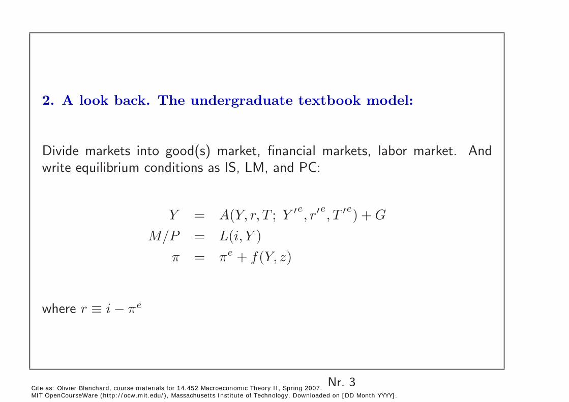
2. A look back. The undergraduate textbook model:

Divide markets into good(s) market, financial markets, labor market. And write equilibrium conditions as IS, LM, and PC:

Y = A(Y, r, T ; Y �e , r�e, T �e) + G

M/P = L(i, Y ) π = πe + f(Y, z)

where r ≡ i − πe


Implications:

• In the SR: Price level is given. IS-LM determines output. Demand matters. Many factors affect demand.

In the MR (reserve “long run” to growth): πe = π, so f(Y, z) = 0.• Output at the natural level.

Money affects output in the SR, not in the MR.•

Money growth affects inflation and the nominal rate one for one in the • MR.

A fiscal expansion increases output in the SR, may decrease it in the• MR.

• Expectations matter. An anticipated fiscal contraction can be expansionary. Effect of money depends on i, πe, i�, π�e

.


What is right, what is wrong with this model, and its many extensions (two goods: investment/consumption, tradables/tradables, home/foreign, more assets, and so on)?

Strength: Simple way of thinking about complex GE. Implicit micro• foundations (life cycle, q theory,...) Time-tested shortcuts.

Weakness: Same. What do the shortcuts short cut? Art versus science. •

More importantly: Without explicit micro-foundations, harder to do wel• fare.

Faced with an increase in the price of oil, what should the Fed try to achieve?

If consumers decrease saving, leading to current account deficit, should fiscal policy be used?


So major reconstruction. Three steps. •

– RBC models.

– Then, introduction of money.

– Then, introduction of nominal rigidities. NK models.

• At the end: Not a very different picture. But better sense of role of distortions. Of optimal policy.

Still a long way to go. Imperfections in labor, financial, goods markets. • Sources of shocks. 14.453, 14.454 (and 14.461, 14.462...)


Topic 1. Stylized Facts.

Want to know:

How long do booms/recessions last? •

How do C, I move with output? •

How does nominal/real money stock move with output? •

How do nominal/real interest rates move with output? •

How do real wages move with output? •

(A OECD/US-centric focus. For emerging countries, see Aguiar-Gopinath).


Have to take up two statistical issues.

1. Covariance stationarity

Little hope of finding regularities if things do not repeat themselves in someway. Right concept is covariance stationarity.Let Yt be a random variable or a vector of random variables. Then, Yt iscovariance stationary iff:

EYt = µ for all t

E(Yt − µ)(Yt−k − µ) = gk for all t

If so, can actually learn/estimate the moments, the stochastic process, the cross-correlations.


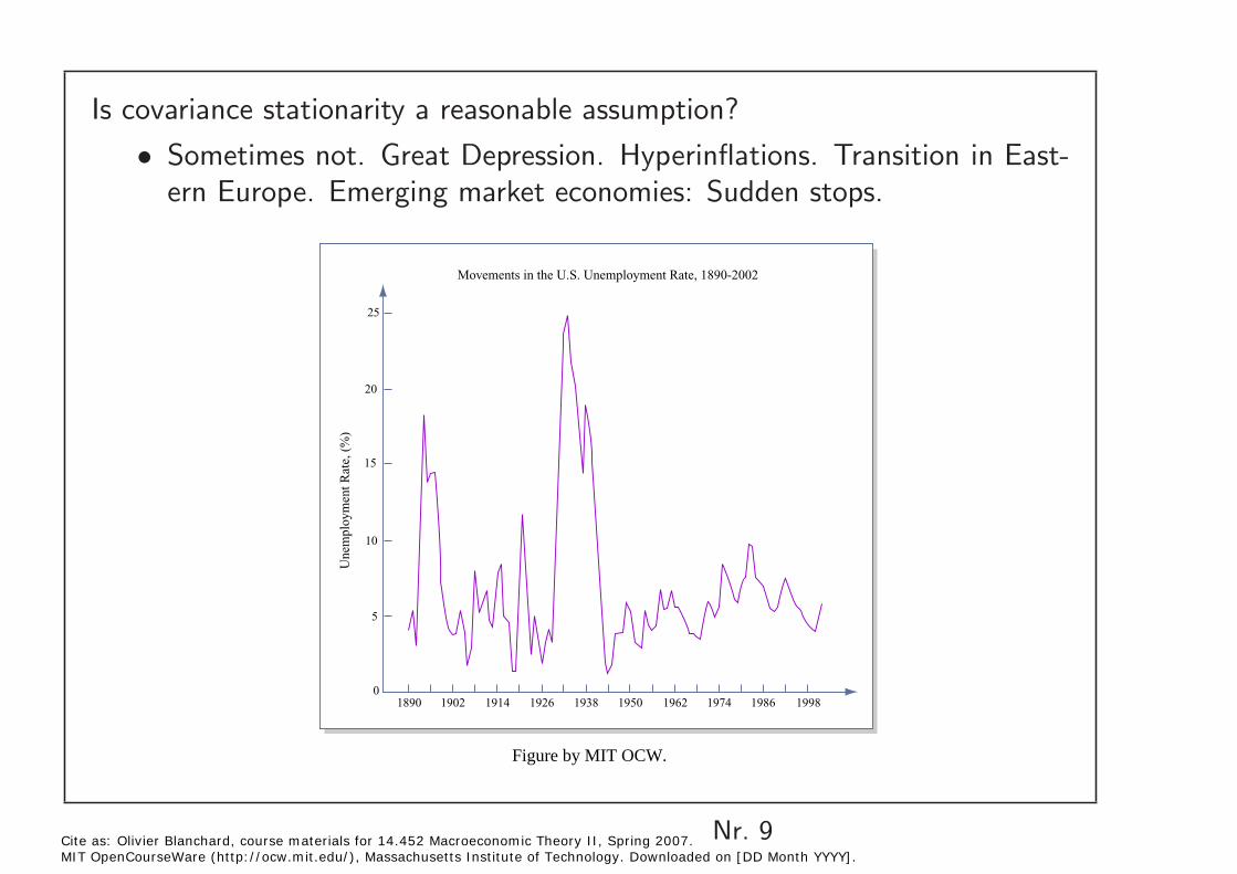
Is covariance stationarity a reasonable assumption?

• Sometimes not. Great Depression. Hyperinflations. Transition in Eastern Europe. Emerging market economies: Sudden stops.

Movements in the U.S. Unemployment Rate, 1890-2002

1890 1902 1914 1926 1938 1950 1962 1974 1986 19980

5

10

15

20

25

Une

mpl

oym

ent R

ate,

(%

)

Figure by MIT OCW.

Nr. 9Cite as: Olivier Blanchard, course materials for 14.452 Macroeconomic Theory II, Spring 2007. MIT OpenCourseWare (http://ocw.mit.edu/), Massachusetts Institute of Technology. Downloaded on [DD Month YYYY].

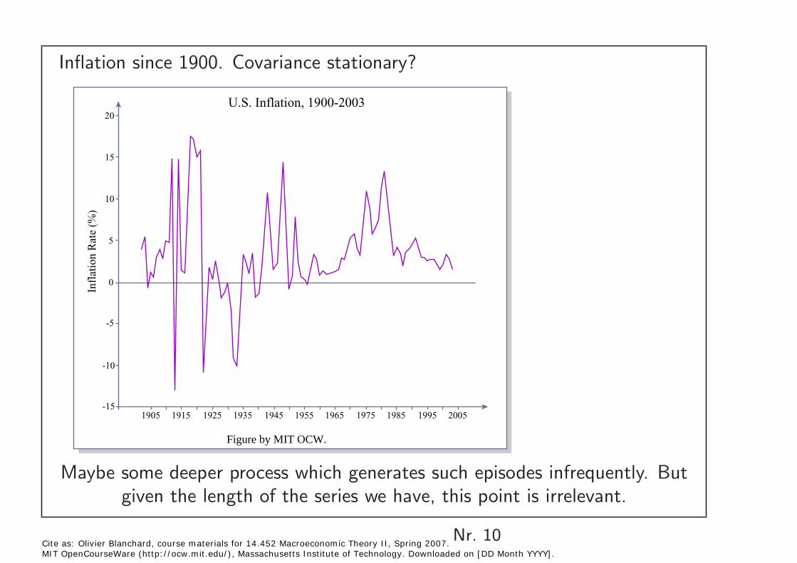
Inflation since 1900. Covariance stationary?In

flat

ion

Rat

e (%

) U.S. Inflation, 1900-2003

20

15

10

5

0

-5

-10

-15 1905 1915 1925 1935 1945 1955 1965 1975 1985 1995 2005

Figure by MIT OCW.

Maybe some deeper process which generates such episodes infrequently. Butgiven the length of the series we have, this point is irrelevant.


1.8

1.6

1.4

1.2

1.0

0.8

0.6

0.4

0.2 1950 1960 1970 1980 1990 2000 2010

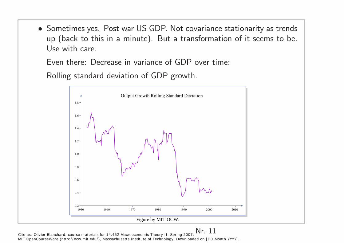
Output Growth Rolling Standard Deviation

Sometimes yes. Post war US GDP. Not covariance stationarity as trends • up (back to this in a minute). But a transformation of it seems to be.Use with care.

Even there: Decrease in variance of GDP over time:

Rolling standard deviation of GDP growth.

Figure by MIT OCW.


Wold decomposition, MAs and ARMAs

If Yt is covariance stationary, then it can be represented by a Wold decomposition (an infinite MA representation):

Yt = �

ψj �t−j + k(t) j

where � is iid, mean 0, constant variance.

• May not be the true process generating movements in Yt. Many shocks. True process may be highly non linear (even deterministic. examples: chaos. Markov processes). Even in those cases, there is an infinite MA Wold representation.

(Why the deterministic component? Typically the mean. More exotic possibilities)

Cite as: Olivier Blanchard, course materials for 14.452 Macroeconomic Theory II, Spring 2007. Nr. 12MIT OpenCourseWare (http://ocw.mit.edu/), Massachusetts Institute of Technology. Downloaded on [DD Month YYYY].

• Very convenient. Infinite MAs cannot be estimated. But they can be approximated quite well by ARMA(n,m) process, or even AR(n) process. Easy to estimate.

Example: AR(1):

Yt = ρYt−1 + �t

• Same if Y and � are vectors. (multivariate) VARs.

Yt = A1Yt−1 + A2Yt−2 + ... + �t

Then, can look at correlations, cross correlations, regression coefficients, and so on. (Stock Watson JEP 2001 for an intro)


Can also think of this as the reduced form of a linear structural model • with shocks. For example, of a model of the form:

Yt = CYt + B1Yt−1 + ... + ut

where C, B1 and so on are matrices of structural parameters, and the ut’s are structural shocks.

ut = (I − C)�t

If recover ut from �t (through identification restrictions), then can trace the effects of ut. Called a “structural VAR”.


2. Trends

Many economic time series trend up. So must deal with/remove the trend. Not a statistical, but an economic issue.

Example 1. A warning. Suppose a variable follows (in logs):

Yt = d + Yt−1 + �t

Random walk with drift. (no return to an underlying trend line)No clean separation between trend and cycle. If fit ex-post a deterministictrend, deviation is garbage. (Fitting trends to stock prices)


Example 2.

Yt = Tt + Ct

Tt = d + Tt−1 + eTt

Ct = aCt−1 + eCt

Can we separate the trend and the cycle components?

• Yes, if eT and eC are uncorrelated, or are perfectly correlated (see Stock and Watson 1988 JEP) Reasonable? Typically not.


• Or if eT has small variance. Then, can hope to get the trend out by taking out a smooth curve: Linear or quadratic trend. Or an HP filter:

t1

min �

((Yt − Tt)2 + λ[(Tt − Tt−1) − (Tt1 − Tt−2)]

2) t0

The larger the parameter λ, the smoother the trend. How to choose λ?

Warning: Trend and by implication the cyclical component depends on future values. Using an HP filtered series in a regression is a no-no.

Or look at first differences. Contain mostly the cyclical component, if eTt is small.

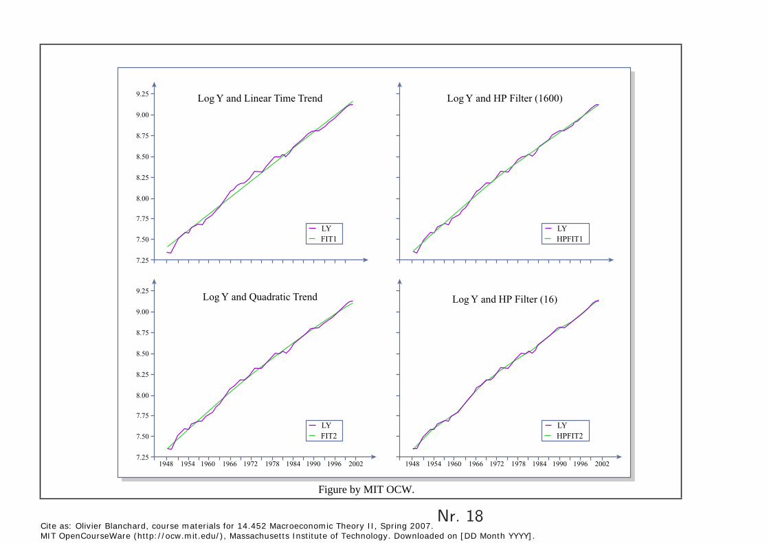
How much of a difference? Results for GDP. Graph.


9.25

9.00

8.75

8.50

8.25

8.00

7.75

7.50

7.25

9.25

9.00

8.75

8.50

8.25

8.00

7.75

7.50

7.25 1948 1954 1960 1966 1972 1978 1984 1990 1996 2002 1948 1954 1960 1966 1972 1978 1984 1990 1996 2002

LY FIT1

LY HPFIT1

LY FIT2

LY HPFIT2

Log Y and Linear Time Trend Log Y and HP Filter (1600)

Log Y and HP Filter (16) Log Y and Quadratic Trend

Figure by MIT OCW.


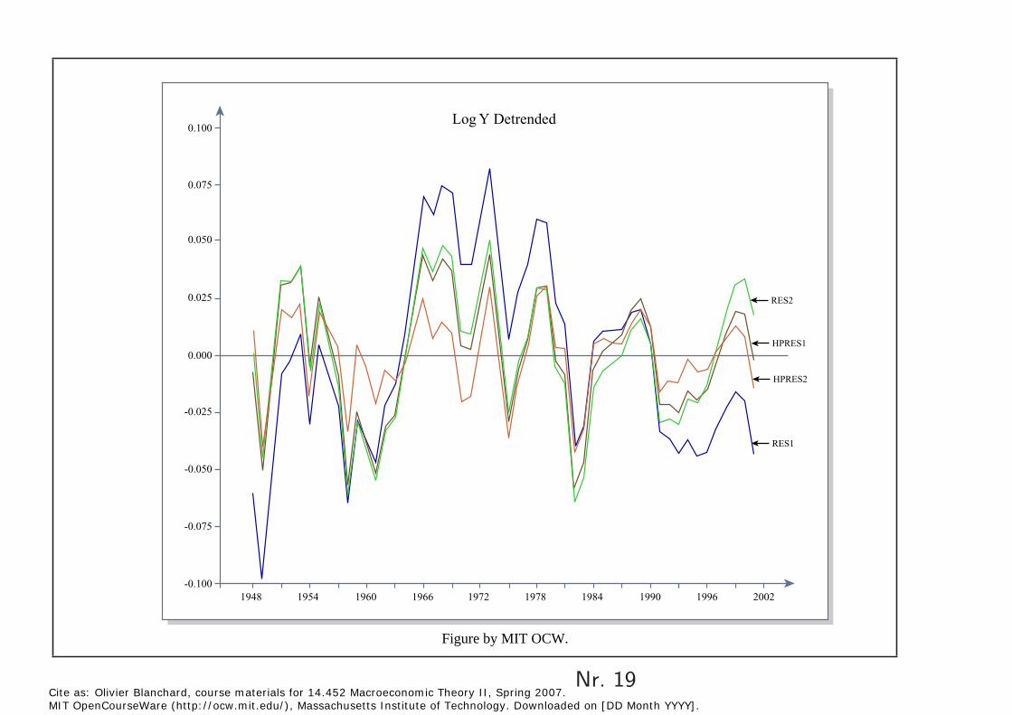
Log Y Detrended 0.100

0.075

0.050

0.025 RES2

HPRES1 0.000

HPRES2

-0.025

RES1

-0.050

-0.075

-0.100 1948 1954 1960 1966 1972 1978 1984 1990 1996 2002

Figure by MIT OCW.


An alternative in the frequency domain (close to HP filter)

Instead of the infinite MA representation, can characterize behavior by thespectrum, giving the importance of the components at different frequencies.

Then, can take out the very low frequencies, perhaps the very high ones. Keep the part of the spectrum corresponding to 6 quarters to 8 years.

This is the Stock-Watson approach (Handbook 1990).


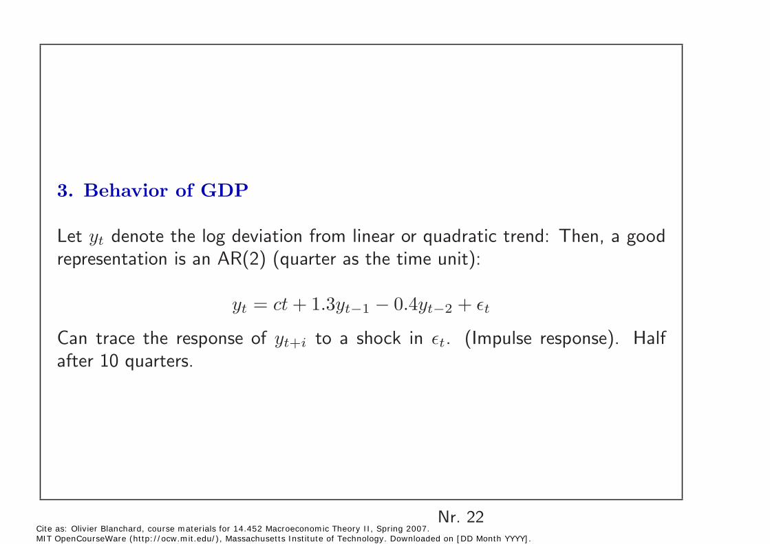
3. Behavior of GDP

Let yt denote the log deviation from linear or quadratic trend: Then, a good representation is an AR(2) (quarter as the time unit):

yt = ct + 1.3yt−1 − 0.4yt−2 + �t

Can trace the response of yt+i to a shock in �t. (Impulse response). Half after 10 quarters.


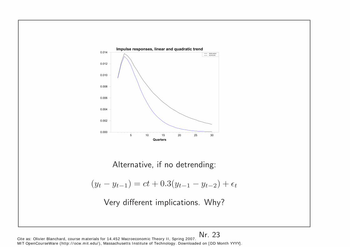
Impulse responses, linear and quadratic trend

Quarters

5 10 15 20 25 30

0.000

0.002

0.004

0.006

0.008

0.010

0.012

0.014RESPLINEAR

RESPQUAD

Alternative, if no detrending:

(yt − yt−1) = ct + 0.3(yt−1 − yt−2) + �t

Very different implications. Why?


4. Co-movements of output with components

Stock Watson, Table 2, looks at the correlation between cyclical components of output and other variables.

ρ(Xct, Yct+k) k = −6, ..., 0, ..., +6

(in quarters)

If ρ is positive and highest for k < 0, then X is procyclical and lags. •

If ρ is positive and highest for k > 0, then X is procyclical and leads. •

(Does not give us a sense of the amplitudes. Covariances rather than correlations would.)


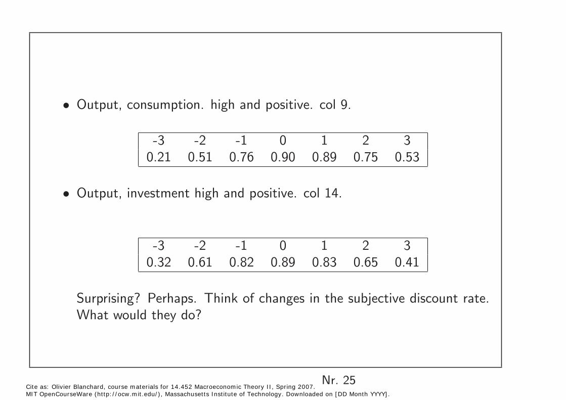
Output, consumption. high and positive. col 9. •

-3 -2 -1 0 1 2 30.21 0.51 0.76 0.90 0.89 0.75 0.53

Output, investment high and positive. col 14. •

-3 -2 -1 0 1 2 30.32 0.61 0.82 0.89 0.83 0.65 0.41

Surprising? Perhaps. Think of changes in the subjective discount rate. What would they do?


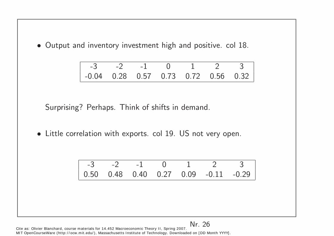
Output and inventory investment high and positive. col 18. •

-3 -2 -1 0 1 2 -0.04 0.28 0.57 0.73 0.72 0.56 0.32

Surprising? Perhaps. Think of shifts in demand.

Little correlation with exports. col 19. US not very open.•

-3 -2 -1 0 1 2 0.50 0.48 0.40 0.27 0.09 -0.11 -0.29


3

3

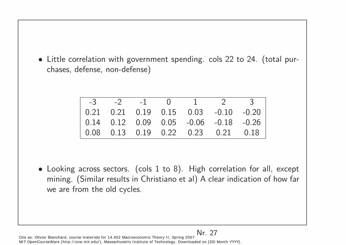
Little correlation with government spending. cols 22 to 24. (total pur• chases, defense, non-defense)

-3 -2 -1 0 1 2 3 0.21 0.21 0.19 0.15 0.03 -0.10 -0.20 0.14 0.12 0.09 0.05 -0.06 -0.18 -0.26 0.08 0.13 0.19 0.22 0.23 0.21 0.18

Looking across sectors. (cols 1 to 8). High correlation for all, except • mining. (Similar results in Christiano et al) A clear indication of how far we are from the old cycles.


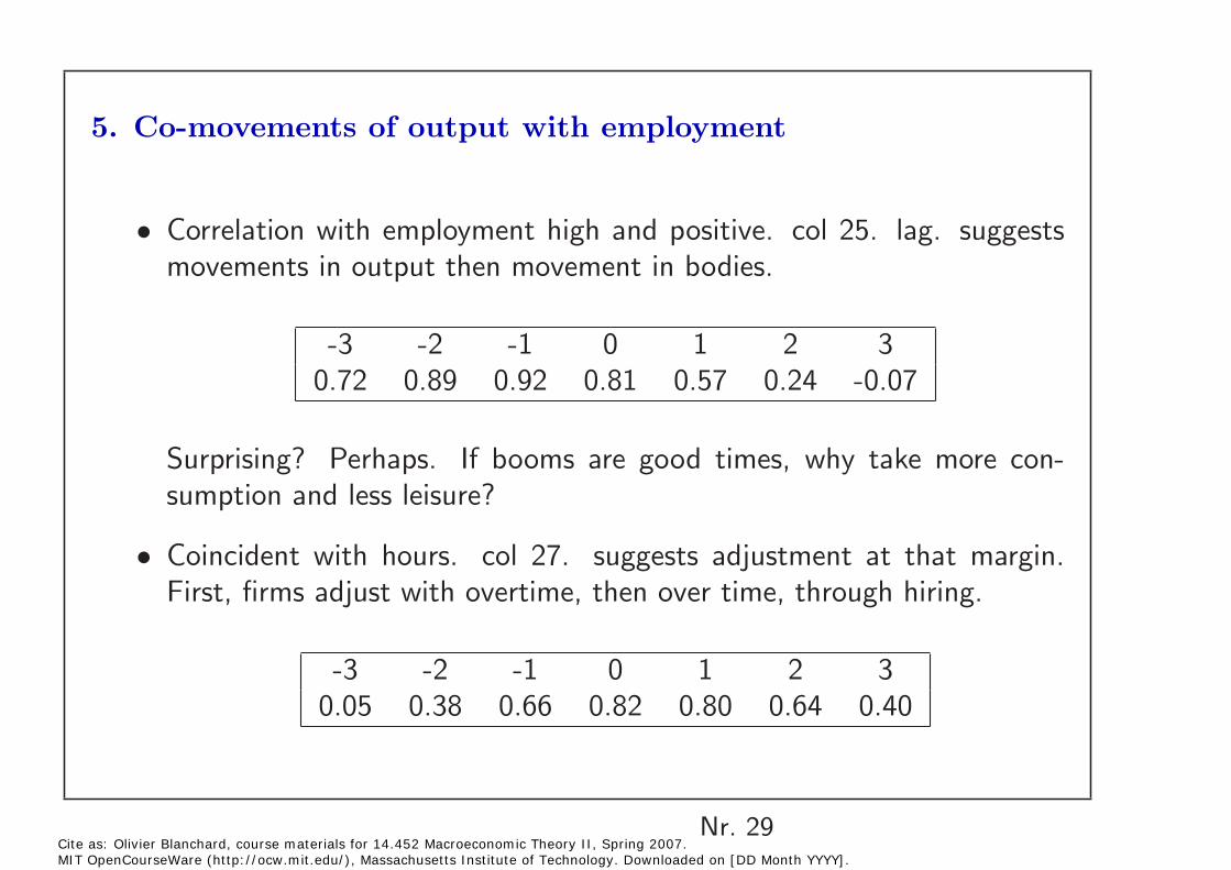
5. Co-movements of output with employment

• Correlation with employment high and positive. col 25. lag. suggests movements in output then movement in bodies.

-3 -2 -1 0 1 2 30.72 0.89 0.92 0.81 0.57 0.24 -0.07

Surprising? Perhaps. If booms are good times, why take more consumption and less leisure?

• Coincident with hours. col 27. suggests adjustment at that margin. First, firms adjust with overtime, then over time, through hiring.

-3 -2 -1 0 1 2 3 0.05 0.38 0.66 0.82 0.80 0.64 0.40


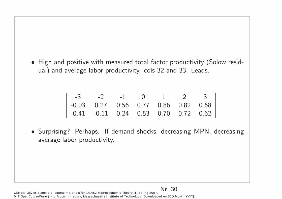
High and positive with measured total factor productivity (Solow resid• ual) and average labor productivity. cols 32 and 33. Leads.

-3 -2 -1 0 1 2 3 -0.03 0.27 0.56 0.77 0.86 0.82 0.68 -0.41 -0.11 0.24 0.53 0.70 0.72 0.62

• Surprising? Perhaps. If demand shocks, decreasing MPN, decreasing average labor productivity.


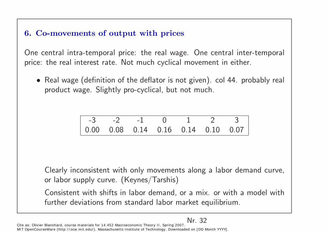
6. Co-movements of output with prices

One central intra-temporal price: the real wage. One central inter-temporal price: the real interest rate. Not much cyclical movement in either.

Real wage (definition of the deflator is not given). col 44. probably real • product wage. Slightly pro-cyclical, but not much.

-3 -2 -1 0 1 2 30.00 0.08 0.14 0.16 0.14 0.10 0.07

Clearly inconsistent with only movements along a labor demand curve, or labor supply curve. (Keynes/Tarshis)

Consistent with shifts in labor demand, or a mix. or with a model with further deviations from standard labor market equilibrium.


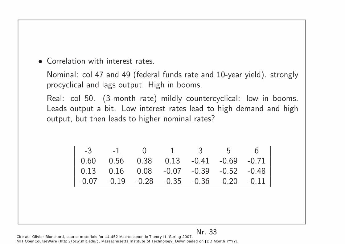
Correlation with interest rates. •

Nominal: col 47 and 49 (federal funds rate and 10-year yield). strongly procyclical and lags output. High in booms.

Real: col 50. (3-month rate) mildly countercyclical: low in booms. Leads output a bit. Low interest rates lead to high demand and high output, but then leads to higher nominal rates?

-3 -1 0 1 3 5 6 0.60 0.56 0.38 0.13 -0.41 -0.69 -0.71 0.13 0.16 0.08 -0.07 -0.39 -0.52 -0.48 -0.07 -0.19 -0.28 -0.35 -0.36 -0.20 -0.11


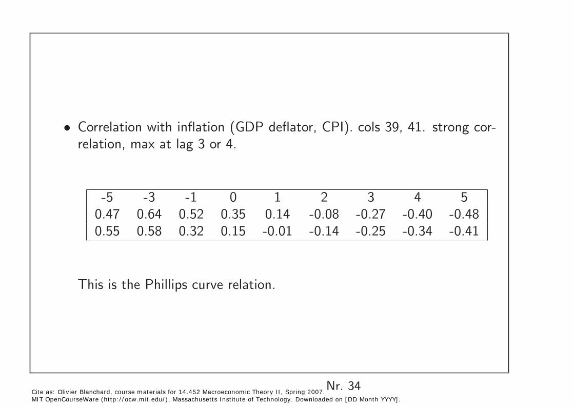
Correlation with inflation (GDP deflator, CPI). cols 39, 41. strong cor• relation, max at lag 3 or 4.

-5 -3 -1 0 1 2 3 4 5 0.47 0.64 0.52 0.35 0.14 -0.08 -0.27 -0.40 -0.48 0.55 0.58 0.32 0.15 -0.01 -0.14 -0.25 -0.34 -0.41

This is the Phillips curve relation.


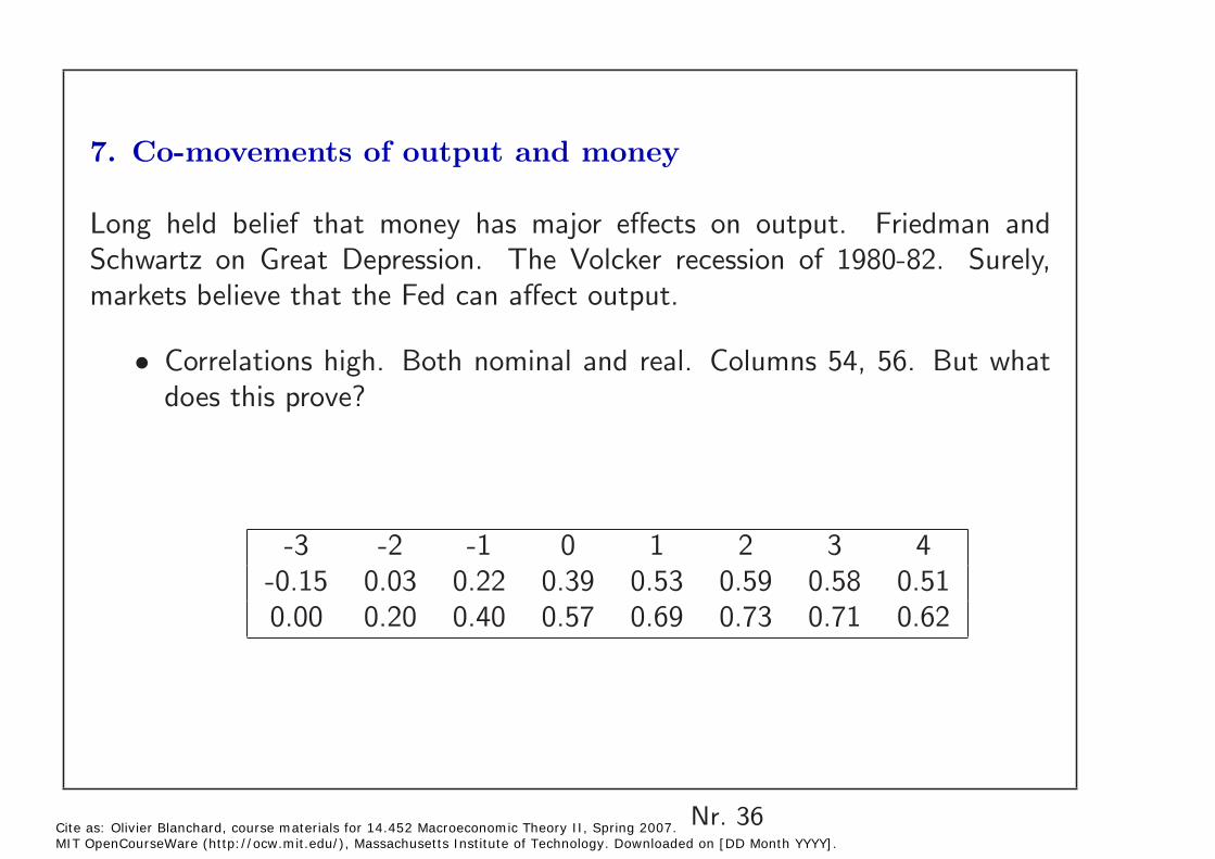
7. Co-movements of output and money

Long held belief that money has major effects on output. Friedman and Schwartz on Great Depression. The Volcker recession of 1980-82. Surely, markets believe that the Fed can affect output.

Correlations high. Both nominal and real. Columns 54, 56. But what • does this prove?

-3 -2 -1 0 1 2 3 4 -0.15 0.03 0.22 0.39 0.53 0.59 0.58 0.51 0.00 0.20 0.40 0.57 0.69 0.73 0.71 0.62


Need more convincing identification. Study by Christiano et al. (based • on a structural VAR)

1% increase in the federal funds rate. remains for about 8 quarters(figure 2). then long lasting effect on output, on employment, on unemployment. Not much effect on the price level until 6 quarters.

How much data mining? See the handbook paper by Christiano, Eichenbaum, Evans.

How convincing? Identifying monetary policy from “exogenous” deviations from the usual rule. Are they really exogenous?

A puzzle: Federal funds rate back to normal far before output is. Notobvious why.


(http://ocw.mit.edu/)

Summary of facts

Components move together •

Procyclical measured productivity •

Not much movement of real wages •

Relation with inflation •

Monetary policy appears to affect output, not prices in the short run. •

Then all the special episodes. Japan Argentina. Asian crisis. Mexico. European unemployment. And so on, working back in time.


Olivier Blanchard April 2007 - MIT OpenCourseWare · 14.452. Topic 1. Introduction and Basic Facts...

Documents

Transcript of Olivier Blanchard April 2007 - MIT OpenCourseWare · 14.452. Topic 1. Introduction and Basic Facts...