Policy Research Working Paper 6603

Oil Price Volatility, Economic Growth and the Hedging Role of Renewable Energy

Jun E. Rentschler

The World BankSustainable Development NetworkOffice of the Chief Economist September 2013

WPS6603P

ublic

Dis

clos

ure

Aut

horiz

edP

ublic

Dis

clos

ure

Aut

horiz

edP

ublic

Dis

clos

ure

Aut

horiz

edP

ublic

Dis

clos

ure

Aut

horiz

edP

ublic

Dis

clos

ure

Aut

horiz

edP

ublic

Dis

clos

ure

Aut

horiz

edP

ublic

Dis

clos

ure

Aut

horiz

edP

ublic

Dis

clos

ure

Aut

horiz

ed

Produced by the Research Support Team

Abstract

The Policy Research Working Paper Series disseminates the findings of work in progress to encourage the exchange of ideas about development issues. An objective of the series is to get the findings out quickly, even if the presentations are less than fully polished. The papers carry the names of the authors and should be cited accordingly. The findings, interpretations, and conclusions expressed in this paper are entirely those of the authors. They do not necessarily represent the views of the International Bank for Reconstruction and Development/World Bank and its affiliated organizations, or those of the Executive Directors of the World Bank or the governments they represent.

Policy Research Working Paper 6603

This paper investigates the adverse effects of oil price volatility on economic activity and the extent to which countries can hedge against such effects by using renewable energy. By considering the Realized Volatility of oil prices, rather than following the standard approach of considering oil price shocks in levels, the effects of factor price uncertainty on economic activity are analyzed. Sample countries represent developed and developing, oil importing and exporting and service/industry-based economies (United States, Japan, Germany, South Korea, India, and Malaysia) and thus complement the standard literature’s analysis of Western OECD countries. In a vector auto-regressive setting, Granger causality tests, impulse response functions, and variance decompositions show that oil price volatility has more-adverse effects in all sample countries than oil price shocks alone can explain. The paper finds

This paper is a product of the Office of the Chief Economist, Sustainable Development Network. It is part of a larger effort by the World Bank to provide open access to its research and make a contribution to development policy discussions around the world. Policy Research Working Papers are also posted on the Web at http://econ.worldbank.org. The author may be contacted at contact@junrentschler.com.

that the sensitivity to oil price volatility varies widely across countries and discusses various factors which may determine the level of sensitivity (such as sectoral composition and the energy mix). This implies that the standard approach of solely considering net oil importer-exporter status is not sufficient. Simulations of volatility shocks in hypothetical energy mixes (with increased renewable shares) illustrate the potential economic benefits resulting from efforts to disconnect the macroeconomy from volatile commodity markets. It is concluded that expanding renewable energy can in principle reduce an economy’s vulnerability to oil price volatility, but a country-specific analysis would be necessary to identify concrete policy measures. Overall, the paper provides an additional rationale for reducing exposure and vulnerability to oil price volatility for the sake of economic growth.

Oil Price Volatility, Economic Growth and the Hedging Role of Renewable Energy

Jun E. Rentschler1,2

Keywords: Oil Price Volatility, Economic Growth, Renewable Energy, Risk Management JEL Classification: C32, C51, Q42, Q43 Sector Board: Energy and Mining (EM)

1 The World Bank, Sustainable Development Network, Office of the Chief Economist, Washington D.C., USA 2 University College London, Dept. of Economics, Energy Institute, 30 Gordon Street, London, WC1H 0AX, UK The author would like to thank John Besant-Jones, Marianne Fay, Stéphane Hallegatte, Malcolm Pemberton, Ingo Rentschler and Janna Tenzing for useful comments on an earlier version of this paper. Remaining errors are the author’s.

2

1. Introduction

As crude oil arguably constitutes one of the single most important driving forces of the global economy, oil price fluctuations are bound to have significant effects on economic growth and welfare. Indeed, the level of oil dependency of industrialized economies became particularly clear in the 1970s and 1980s, when a series of political incidents in the Middle East disrupted the security of supply and had severe effects on the global price of oil. Since then oil price shocks have continuously increased in size and frequency. While demand for oil is likely to remain relatively slow moving, mainly driven by economic growth and to some extent climate policies, supply will remain highly uncertain, not least considering persistent instability in exporting countries and the uncertainty regarding the discovery of new resources. As a result of such uncertainties, and in the context of today’s tightly traded markets, future oil prices are also expected to undergo (increasingly) drastic fluctuations. Theoretically, an oil price shock can be transmitted into the macro-economy via various channels. Principally, a positive oil price shock will increase production costs and hence restrict output (henceforth denoted as ‘input channel’) (Barro, 1984). Energy intensive industrial production will be more affected than service based industries. A prolonged oil price increase will necessitate costly structural changes to production processes with potentially adverse employment effects. However, it is crucial to note that the frequency of oil price shocks (both positive and negative) increases perceived price uncertainty. According to Bernanke (1983), such oil price volatility will reduce planning horizons and cause firms to postpone irreversible business investments (‘uncertainty channel’).

Due to countless possible exogenous supply shocks, oil prices are subject to uncertainty at any point in time. Even when prices remain relatively stable over an extended period of time, a sudden exogenous event could disrupt the balance independently of previous events and cause significant upward or downward price changes (e.g. a large earthquake may reduce economic activity and the demand for crude oil accordingly, hence reducing prices). When prices are stable, economic agents (incl. households, firms and governments) tend to overlook the ubiquitous, permanent underlying uncertainty, when making economic decisions. However, in an environment of already volatile prices, agents are more likely to take future price uncertainty into account when making investment decisions. Overall, oil price volatility typically results in an increased sense of economic uncertainty, whereas the absence of volatility may instill a false sense of stability. They are however not interchangeable terms, as uncertainty can exist in the absence of volatility.

In order to hedge against negative effects of oil price volatility, it is of utmost importance for policy makers to understand how significant the potential dimensions of negative effects are, and which factors determine the level of vulnerability. While there exists significant literature establishing a negative and asymmetric relationship between oil price shocks and macro-economic indicators, research has focused on actual oil price shocks rather than price volatility (and accordingly uncertainty) directly. Furthermore, emerging economies and their country specific parameters have largely been overlooked. Little has been said about why sensitivity differs across countries, and why some net exporters benefit from oil price fluctuations, while others suffer. This paper addresses these shortcomings. Like the vast majority of literature on this topic, this paper considers real, exchange rate adjusted oil prices and does not take into account taxation.

2. The Oil-GDP Literature – Review of Empirical Evidence

Given the crucial role of crude oil in the global economy, the relationship between oil prices and economic activity has received considerable attention by economists since the early 1980s. Hamilton (1983) notes that seven of eight recessions in the period 1948 to 1980 were preceded by significant oil price increases and hence establishes a causal oil-price-GDP link for the USA. Subsequently these findings were confirmed by Burbidge and Harrison (1984), Gisser and Goodwin (1986), Mork (1989), Ferderer (1996) and others. Corresponding studies for other major OECD countries by Mork et al. (1994), Papapetrou (2001), Jiménez-Rodríguez and Sanchez (2005) and Lardic and Mignon (2006) revealed that the negative oil-price-GDP effect prevails in virtually all industrialized economies. Furthermore, oil price volatility has also been shown to have significant impacts on stock market returns (Filis et al., 2011), and bilateral trade (Chen and Hsu, 2013). Findings are surprisingly similar across developed countries and extend to both net importers and exporters (e.g. UK) of oil (Mork et al. 1994). Blanchard and Gali (2007) also recognize the economic sensitivity to oil shocks, but suggest that industrialized countries have become less sensitive since the 1970s for various reasons, including reduced reliance on oil as an input factor to industrial production.

3

Due to limited availability of data, the majority of existing literature analyzes the oil-price-GDP relationship in major OECD economies. However, Japan and the emerging economies in South East Asia have been largely omitted from the discussion. Notable exceptions are Lee et al. (2001) who study the impact of oil price shocks on Japanese monetary policy and macro-economy; as well as Cunado and Gracia (2005) who conduct cointegration and Granger causality tests for six Asian economies3. They find that there exists no long-run cointegrating relationship between oil prices and economic growth, but oil prices indeed Granger cause economic growth in the short-run. With these results Cunado and Gracia (2005) verify the existence of a significant negative oil-GDP relationship in Asian developing countries – including Malaysia, a net oil exporter. Notably, Guo and Kliesen (2005) differ from the existing literature by constructing the ‘Realized Volatility’ (RV) variable suggested by Andersen et al. (2004), rather than employing the standard method of considering oil price shocks directly. This allows them to account for the input channel as well as the uncertainty channel (cf. Section 1). Using the same realized volatility measure, Rafiq et al. (2009) extend Cunado and Gracia’s (2005) study by analyzing the effects of oil price volatility for various macro-indicators in the Thai economy. In a vector auto-regression (VAR) and vector error correction model, they show that the realized volatility of oil prices Granger causes GDP growth, investment, unemployment and inflation. Impulse response functions confirm that impacts of realized volatility are most distinct in the short-run, particularly for GDP. This result, together with the variance decomposition, supports Bernanke’s (1983) theoretical explanation of postponed investments due to expected oil price volatility and the associated uncertainty.

To understand the nature of the oil-GDP relationship, it is crucial to consider the existence of asymmetry, i.e. adverse effects of oil price increases exceed stimulating effects of oil price decreases. However, the empirical evidence for the nature of this asymmetry is ambiguous. While it is generally agreed that increases have adverse effects, evidence for the effects of decreases is far from conclusive. Mork (1989) distinguishes between positive and negative oil price shocks and finds that oil price increases reduce GDP while decreases have hardly any impact. However, Mork et al. (1994) find that oil price increases and decreases both have negative consequences for the US economy, while results for the UK, Japan, France, Norway, Germany and Canada are inconclusive. Mory (1993) and Lee et al. (1995) find that oil price decreases have no impact on the US economy. Lardic and Mignon (2006) show that standard cointegration is rejected for most of the twelve European sample countries, while asymmetric cointegration is determined to be of major relevance in explaining the impact of oil price shocks. The underlying reasoning is that asymmetry is caused by asymmetric monetary policy, i.e. more drastic policy measures in response to oil price increases, than to decreases (Hamilton and Herrera, 2004). Ferderer (1996) indeed confirms a strong link between oil price shocks and monetary policy responses, but nevertheless argues that oil prices Granger cause GDP directly. Hence he concludes that asymmetric monetary policy alone is not sufficient to account for the asymmetric oil-GDP relationship. In addition to monetary policy, downward stickiness of wages and prices due to, e.g. institutional regulation or contractual commitments, is a standard explanation for asymmetric effects. For the purposes of this study asymmetry is of major importance: While in a symmetric scenario a positive and a negative oil price shock would cancel each other, in an asymmetric setting the presence of price movements (i.e. volatility) per se will impact on economic indicators.

3. Methodology and Empirical Evidence

3.1. Data

The selected sample represents developed/developing, oil importing/exporting and service/industry based economies. The USA is the by far largest consumer of petroleum and at the same time has considerable domestic production. The third and fourth largest economies, Japan (JPN) and Germany (GER), have had (at least until recently) strong surplus economies, led by exports and industrial production. This industry structure, as well as negligible domestic oil production make Japan and Germany highly dependent on petroleum imports. Furthermore, a set of ‘leaping’ economies is selected, namely India (IND), South Korea (KOR) and Malaysia (MYS), as they have experienced immense economic growth throughout the considered data period (1983-2011). As numerous developing countries are resource rich oil exporters, it is of particular importance to include Malaysia, a net oil exporter.

3 Japan, Malaysia, Philippines, Singapore, South Korea and Thailand

4

For the purposes of this study, economic activity constitutes the dependent variable and oil price volatility the key regressor. While the overwhelming majority of literature in this field uses quarterly data, this study uses monthly data, in order to capture intra-quarter volatility. Monthly industrial production (IP) is used as a proxy for economic activity, as it is particularly sensitive to changes in input prices (such as oil). Industrial production series and consumer price indices are obtained from the IMF Intl. Finance Statistics database and seasonally adjusted4. A ‘global oil price’ is obtained by deflating an average of the WTI and Brent spot market prices (in USD/barrel) using a price index for non-fuel primary commodities. To obtain a more accurate measure of the domestically ‘perceived’ oil price, the global oil price is adjusted for the respective country’s daily $-exchange rate and inflation. Hence, for each country a time series of continuous daily oil prices 𝜋𝑑 is obtained, with 𝑑 𝜖 𝑇𝑑, where 𝑇𝑑 = [June, 1. ,1983; June, 2. ,1983; . . . , ; Jan. ,31. ,2011]; i.e. 7017 observations. It should be noted that adjusting global oil prices for domestic exchange rate and inflation effects is common practice in this literature (see for instance Mork et al., 1994 and Abeysinghe, 2001) – however it should also be pointed out that such domestic oil prices reflect the perceived prices before any kind of policy intervention. In practice oil prices tend to be distorted further through fiscal policies, such as taxes or subsidies (for a detailed discussion of fuel pricing see Kojima, 2013).

Figure 1. Domestic real oil prices (left axis) in domestic currency per barrel (e.g. EUR/BBL) and global real oil price (right axis, in USD/BBL).

Figure 1 illustrates that oil prices have undergone considerable fluctuations in the period 1983-2011, with the global nominal oil price varying between US$ 145.7 (03/07/2008) and US$ 8.7 (25/07/1986) with a standard deviation of US$ 25.7 5. Evidently, there exists a strong correlation between all six domestic pre-tax oil prices, as well as between domestic and global oil prices (cf. Table 1.). This confirms that most of the variation in ‘perceived’ oil prices is indeed due to global oil price shocks, even though domestic effects can play a significant role. The correlation between post-tax oil prices is likely to differ, particularly for countries such as Malaysia with significant fuel subsidy schemes in place.

4 Seasonal adjustment using the X-12 method. 5 In real terms: max. US$ 86.3 (03/07/2008), min. US$ 11.1 (25/07/1986), S.D. US$ 14.6

020406080100120140160180

-50-40-30-20-10

01020304050607080

'83 '86 '89 '92 '95 '98 '01 '04 '07 '10

Germany (EUR/BBL)

020406080100120140160180

-100-80-60-40-20

020406080

100120140160

'83 '86 '89 '92 '95 '98 '01 '04 '07 '10

USA (USD/BBL)

020406080100120140160180

-10000-8000-6000-4000-2000

02000400060008000

1000012000140001600018000

'83 '86 '89 '92 '95 '98 '01 '04 '07 '10

Japan (JPY/BBL)

020406080100120140160180

-80000-60000-40000-20000

020000400006000080000

100000120000140000160000

'83 '86 '89 '92 '95 '98 '01 '04 '07 '10

S.Korea (KRW/BBL)

020406080100120140160180

-2000-1000

0100020003000400050006000

'83 '86 '89 '92 '95 '98 '01 '04 '07 '10

India (INR/BBL)

020406080100120140160180

-200-150-100-50

050

100150200250300350400450

'83 '86 '89 '92 '95 '98 '01 '04 '07 '10

Malaysia (MYR/BBL)

5

World USA JPN GER IND KOR MYS World 1 0.941 0.841 0.876 0.965 0.919 0.979 USA

1 0.960 0.958 0.929 0.971 0.946

JPN

1 0.964 0.858 0.941 0.874 GER

1 0.887 0.965 0.907

IND

1 0.899 0.978 KOR

1 0.927

MYS

1

Table 1. Correlation coefficients between domestic and global oil prices

Following the above notation the daily change in the price of crude oil is denoted 𝜌𝑑, where

𝜌𝑑 = 𝜋𝑑 − 𝜋𝑑−1

𝜋𝑑−1.

Computing daily changes for all six countries respectively reveals a pattern similar to the daily changes in the global oil price, depicted in Figure 3. The mean daily oil price change is not found to be significantly different from zero. Following Hamilton (1983), the oil price 𝜋𝑑 can be modeled as a random walk process,

𝜋𝑑 = 𝑐 + 𝜋𝑑−1 + 𝑢𝑑

where the innovation 𝑢𝑑 = 𝜎𝜀𝑑, with 𝜀𝑑~ iid 𝒩(0,1). The Ljung-Box test for squared residuals, confirms all six oil price return series to be following an autoregressive conditional heteroskedasticity (ARCH) process. This is graphically confirmed by Figure 3, in which distinct high volatility clusters are evident (e.g. 1986, 1990, 2008).

3.2. Realized Volatility

From 1947 to 1986, oil prices remained (relatively) stable, whereby shocks were almost exclusively positive and moderate in size. However, since the mid-1980s, oil prices have undergone substantial positive and negative shocks. The classical approach, such as by Mork (1989), which considers oil price innovations in levels, fails to remain statistically significant in subsequent sample periods. Subsequently, various studies (Hamilton, 1996, 2003; Hooker, 1996) found direct measures of volatility to be more powerful in explaining the oil-GDP relationship than oil prices in levels. Based on this, this study employs the Realized Volatility (RV) measure as suggested by Andersen et al. (2003). Drawing on conventional finance literature, a price process 𝜋𝑡 is expressed as a stochastic differential equation:

𝑑log (𝜋𝑡) = 𝜇𝑡𝑑𝑡 + 𝜎𝑡𝑑𝒲𝑡

where 𝜇𝑡 denotes a predictable drift term with finite variance, 𝜎𝑡 corresponds to volatility and 𝒲𝑡 denotes standard Brownian Motion. The continuously compounded price change 𝑟𝑡 in the unit time interval is denoted

𝑟𝑡 ≡ log (𝜋𝑡) − log (𝜋𝑡−1) = � 𝜇𝑢𝑑𝑢𝑡

𝑡−1+ � 𝜎𝑢𝑑𝒲𝑢

𝑡

𝑡−1

-80-60-40-20

020406080

1947

1950

1953

1956

1959

1962

1965

1968

1971

1974

1977

1980

1983

1986

1989

1992

1995

1998

2001

2004

2007

2010

2013

-0.4-0.3-0.2-0.1

00.10.20.30.4

1983

1985

1987

1989

1991

1993

1995

1997

1999

2001

2003

2005

2007

2009

2011

Figure 3. Daily global oil price changes 1983-2011 – similar patterns for all countries.

Figure 2. Percentage change in the quarterly price of crude oil (Source: Dow Jones & Co., Thomson Reuters)

6

where 𝑡 − 1 ≤ 𝑢 ≤ 𝑡. First and second moments are obtained, based on the assumption that 𝑑𝜎𝑢 and 𝑑𝒲𝑢 are uncorrelated (no leverage effect). Since standard Brownian Motion has increments distributed according to 𝑊𝑡 −𝑊𝑠 ~ 𝒩(0, 𝑡 − 𝑠) for 0 ≤ 𝑠 ≤ 𝑡, the mean of 𝑟𝑡 conditional on information set Ω 𝑡−1 is given by

𝔼{𝑟𝑡|Ωt−1} = � 𝜇𝑢𝑑𝑢𝑡

𝑡−1.

Accordingly, conditional variance, or Integrated Volatility 𝐼𝑉𝑡 , is given by

𝑉𝑎𝑟{𝑟𝑡|Ωt−1} ≡ 𝐼𝑉𝑡 = � 𝜎𝑢2𝑑𝑢.𝑡

𝑡−1

Of course, return and volatility computations in practice are restricted to discrete time intervals, hence 𝐼𝑉𝑡 is latent and can only be approximated. As parametric models of estimating 𝐼𝑉𝑡 are prone to misspecification, an elegant non-parametric method is to estimate volatility of daily changes by a monthly realized volatility series6. Realized volatility is defined as the summation of squared daily changes over the period from the first to the last day (𝐷𝑚) of a given month:

𝑅𝑉𝑚(𝜌𝑑) = � 𝜌𝑑2 =𝐷𝑚

𝑑=1� �

𝜋𝑑 − 𝜋𝑑−1𝜋𝑑−1

�2𝐷𝑚

𝑑=1,

where 𝑅𝑉𝑚(𝜌𝑑) denotes the monthly realized volatility of daily changes 𝜌𝑑. Crucially, based on the quadratic variation theory, Andersen et al. (2004) demonstrate that a volatility measure 𝑅𝑉𝑝(𝑥) converges uniformly in probability to 𝐼𝑉𝑡 as 𝑝 → 0; and hence is an unbiased and efficient estimator7. In practice, increasing the sampling frequency of intra-period changes will yield a more accurate non-parametric estimator of 𝐼𝑉𝑡. This study will therefore be based on monthly data, unlike Guo and Kliesen (2005) and Rafiq et al. (2009), who measure oil price variance only at quarterly frequency, and hence ‘aggregate away’ potentially valuable information on intra-quarter volatility.

Figure 4. Monthly Realized Volatility (1983 – 2011). Distinct clusters of high volatility are evident, even though their extent varies across countries due to exchange rate and inflation effects.

6 While a RV estimate of higher frequency (e.g. daily RV based on intraday price returns) would capture volatility more accurately, this could not reasonably be analysed against lower frequency macro data. In practice, monthly Industrial Production data is the highest frequency proxy for economic growth. 7 Note that Andersen et al. (2004) denote the h-period volatility at date t as 𝑅𝑉𝑡(ℎ), while in this study 𝑅𝑉𝑚(𝜌𝑑) denotes the monthly volatility in month m, based on daily returns 𝜌𝑑.

0.000.050.100.150.200.250.300.35

1983

1985

1987

1989

1991

1993

1995

1997

1999

2001

2003

2005

2007

2009

USA

0.000.020.040.060.080.100.120.140.160.180.20

1983

1985

1987

1989

1991

1993

1995

1997

1999

2001

2003

2005

2007

2009

Germany

0.000.020.040.060.080.100.120.140.160.180.20

1983

1985

1987

1989

1991

1993

1995

1997

1999

2001

2003

2005

2007

2009

Japan

0.000.020.040.060.080.100.120.140.160.180.20

1983

1985

1987

1989

1991

1993

1995

1997

1999

2001

2003

2005

2007

2009

Malaysia

0.000.020.040.060.080.100.120.140.160.180.20

1983

1985

1987

1989

1991

1993

1995

1997

1999

2001

2003

2005

2007

2009

India

0.000.020.040.060.080.100.120.140.160.180.20

1983

1985

1987

1989

1991

1993

1995

1997

1999

2001

2003

2005

2007

2009

S.Korea

7

3.3. Modeling the Volatility-GDP Relationship

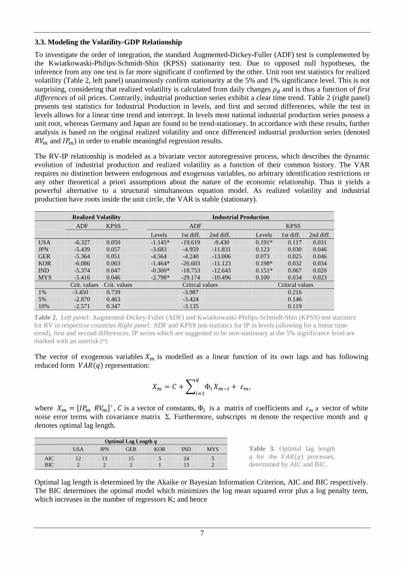
To investigate the order of integration, the standard Augmented-Dickey-Fuller (ADF) test is complemented by the Kwiatkowaski-Philips-Schmidt-Shin (KPSS) stationarity test. Due to opposed null hypotheses, the inference from any one test is far more significant if confirmed by the other. Unit root test statistics for realized volatility (Table 2, left panel) unanimously confirm stationarity at the 5% and 1% significance level. This is not surprising, considering that realized volatility is calculated from daily changes 𝜌𝑑 and is thus a function of first differences of oil prices. Contrarily, industrial production series exhibit a clear time trend. Table 2 (right panel) presents test statistics for Industrial Production in levels, and first and second differences, while the test in levels allows for a linear time trend and intercept. In levels most national industrial production series possess a unit root, whereas Germany and Japan are found to be trend-stationary. In accordance with these results, further analysis is based on the original realized volatility and once differenced industrial production series (denoted 𝑅𝑉𝑚 and 𝐼𝑃𝑚) in order to enable meaningful regression results.

The RV-IP relationship is modeled as a bivariate vector autoregressive process, which describes the dynamic evolution of industrial production and realized volatility as a function of their common history. The VAR requires no distinction between endogenous and exogenous variables, no arbitrary identification restrictions or any other theoretical a priori assumptions about the nature of the economic relationship. Thus it yields a powerful alternative to a structural simultaneous equation model. As realized volatility and industrial production have roots inside the unit circle, the VAR is stable (stationary).

Realized Volatility Industrial Production

ADF KPSS

ADF

KPSS

Levels 1st diff. 2nd diff. Levels 1st diff. 2nd diff.

USA -6.327 0.050

-1.145* -19.619 -9.430

0.191* 0.117 0.031 JPN -5.439 0.057

-3.683 -4.959 -11.831

0.123 0.030 0.046

GER -5.364 0.051

-4.564 -4.240 -13.006

0.073 0.025 0.046 KOR -6.086 0.063

-1.464* -26.603 -11.123

0.198* 0.032 0.034

IND -5.374 0.047

-0.300* -18.753 -12.643

0.151* 0.067 0.020 MYS -5.416 0.046

-2.798* -29.174 -10.496

0.100 0.034 0.023

Crit. values Crit. values Critical values

Critical values

1% -3.450 0.739

-3.987

0.216 5% -2.870 0.463

-3.424

0.146

10% -2.571 0.347

-3.135

0.119

The vector of exogenous variables 𝑋𝑚 is modelled as a linear function of its own lags and has following reduced form 𝑉𝐴𝑅(𝑞) representation:

𝑋𝑚 = 𝐶 + � Φi

𝑞

𝑖=1𝑋𝑚−𝑖 + 𝜀𝑚,

where 𝑋𝑚 = [𝐼𝑃𝑚 𝑅𝑉𝑚]′ , 𝐶 is a vector of constants, Φi is a matrix of coefficients and 𝜀𝑚 a vector of white noise error terms with covariance matrix Σ. Furthermore, subscripts 𝑚 denote the respective month and 𝑞 denotes optimal lag length.

Optimal Lag Length 𝒒 USA JPN GER KOR IND MYS

AIC 12 13 15 5 24 5 BIC 2 2 2 1 13 2

Optimal lag length is determined by the Akaike or Bayesian Information Criterion, AIC and BIC respectively. The BIC determines the optimal model which minimizes the log mean squared error plus a log penalty term, which increases in the number of regressors K; and hence

Table 2. Left panel: Augmented-Dickey-Fuller (ADF) and Kwiatkowaski-Philips-Schmidt-Shin (KPSS) test statistics for RV in respective countries Right panel: ADF and KPSS test statistics for IP in levels (allowing for a linear time trend), first and second differences. IP series which are suggested to be non-stationary at the 5% significance level are marked with an asterisk (*).

Table 3. Optimal lag length 𝑞 for the 𝑉𝐴𝑅(𝑞) processes, determined by AIC and BIC.

8

𝐵𝐼𝐶 = 𝑙𝑜𝑔1𝑁� 𝑒𝑖2 +

𝐾𝑁𝑙𝑜𝑔𝑁

𝑁

𝑖=1

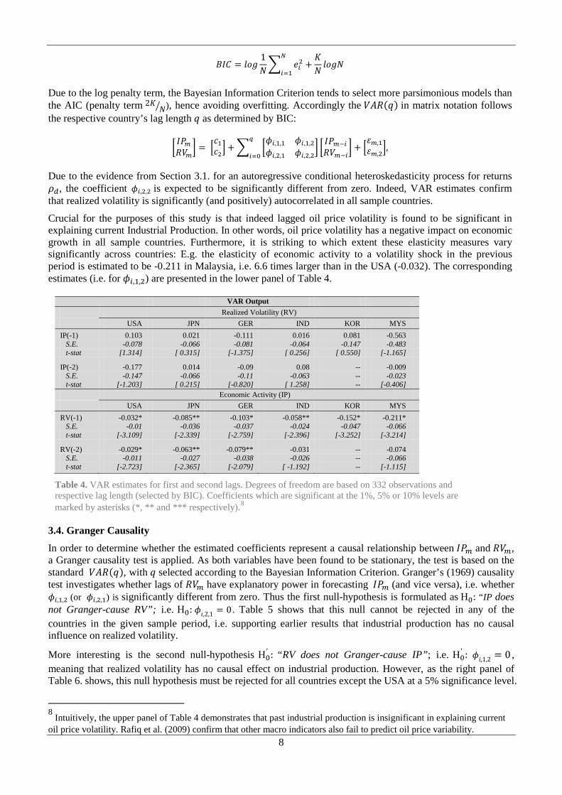
Due to the log penalty term, the Bayesian Information Criterion tends to select more parsimonious models than the AIC (penalty term 2𝐾 𝑁� ), hence avoiding overfitting. Accordingly the 𝑉𝐴𝑅(𝑞) in matrix notation follows the respective country’s lag length 𝑞 as determined by BIC:

� 𝐼𝑃𝑚𝑅𝑉𝑚� = �

𝑐1𝑐2� + � �

𝜙𝑖,1,1 𝜙𝑖,1,2𝜙𝑖,2,1 𝜙𝑖,2,2

�𝑞

𝑖=0� 𝐼𝑃𝑚−𝑖𝑅𝑉𝑚−𝑖

� + �𝜀𝑚,1𝜀𝑚,2

�,

Due to the evidence from Section 3.1. for an autoregressive conditional heteroskedasticity process for returns 𝜌𝑑, the coefficient 𝜙𝑖,2,2 is expected to be significantly different from zero. Indeed, VAR estimates confirm that realized volatility is significantly (and positively) autocorrelated in all sample countries.

Crucial for the purposes of this study is that indeed lagged oil price volatility is found to be significant in explaining current Industrial Production. In other words, oil price volatility has a negative impact on economic growth in all sample countries. Furthermore, it is striking to which extent these elasticity measures vary significantly across countries: E.g. the elasticity of economic activity to a volatility shock in the previous period is estimated to be -0.211 in Malaysia, i.e. 6.6 times larger than in the USA (-0.032). The corresponding estimates (i.e. for 𝜙𝑖,1,2) are presented in the lower panel of Table 4.

VAR Output

Realized Volatility (RV) USA JPN GER IND KOR MYS IP(-1) 0.103 0.021 -0.111 0.016 0.081 -0.563 S.E. -0.078 -0.066 -0.081 -0.064 -0.147 -0.483 t-stat [1.314] [ 0.315] [-1.375] [ 0.256] [ 0.550] [-1.165]

IP(-2) -0.177 0.014 -0.09 0.08 -- -0.009 S.E. -0.147 -0.066 -0.11 -0.063 -- -0.023 t-stat [-1.203] [ 0.215] [-0.820] [ 1.258] -- [-0.406] Economic Activity (IP) USA JPN GER IND KOR MYS RV(-1) -0.032* -0.085** -0.103* -0.058** -0.152* -0.211* S.E. -0.01 -0.036 -0.037 -0.024 -0.047 -0.066 t-stat [-3.109] [-2.339] [-2.759] [-2.396] [-3.252] [-3.214]

RV(-2) -0.029* -0.063** -0.079** -0.031 -- -0.074 S.E. -0.011 -0.027 -0.038 -0.026 -- -0.066 t-stat [-2.723] [-2.365] [-2.079] [ -1.192] -- [-1.115]

Table 4. VAR estimates for first and second lags. Degrees of freedom are based on 332 observations and respective lag length (selected by BIC). Coefficients which are significant at the 1%, 5% or 10% levels are marked by asterisks (*, ** and *** respectively).8

3.4. Granger Causality

In order to determine whether the estimated coefficients represent a causal relationship between 𝐼𝑃𝑚 and 𝑅𝑉𝑚, a Granger causality test is applied. As both variables have been found to be stationary, the test is based on the standard 𝑉𝐴𝑅(𝑞), with 𝑞 selected according to the Bayesian Information Criterion. Granger’s (1969) causality test investigates whether lags of 𝑅𝑉𝑚 have explanatory power in forecasting 𝐼𝑃𝑚 (and vice versa), i.e. whether 𝜙𝑖,1,2 (or 𝜙𝑖,2,1) is significantly different from zero. Thus the first null-hypothesis is formulated as Η0: “IP does not Granger-cause RV”; i.e. Η0: 𝜙𝑖,2,1 = 0. Table 5 shows that this null cannot be rejected in any of the countries in the given sample period, i.e. supporting earlier results that industrial production has no causal influence on realized volatility.

More interesting is the second null-hypothesis Η0′ : “RV does not Granger-cause IP”; i.e. Η0

′ : 𝜙𝑖,1,2 = 0 , meaning that realized volatility has no causal effect on industrial production. However, as the right panel of Table 6. shows, this null hypothesis must be rejected for all countries except the USA at a 5% significance level.

8 Intuitively, the upper panel of Table 4 demonstrates that past industrial production is insignificant in explaining current oil price volatility. Rafiq et al. (2009) confirm that other macro indicators also fail to predict oil price variability.

9

This means that there is statistically significant evidence that oil price volatility RV has a causal impact on economic activity, i.e. contemporary RV is useful in forecasting future industrial production. With respect to the USA it should be noted that the p-value 0.059 is only marginally excessive of the 0.05 significance level. At a 10% (or in fact 6%) significance level the null of ‘no Granger causality’ would also be rejected for the USA.

Granger Causality

Η0: “IP does not Granger cause RV”

Η0′ : “RV does not Granger cause IP”

F-statistic p-value

F-statistic p-value

USA 0.977 0.480

1.589 0.059 JPN 0.829 0.620

2.492 0.004

GER 0.632 0.814

2.053 0.020 KOR 0.230 0.875

2.329 0.009

IND 0.499 0.751

1.565 0.048 MYS 0.499 0.683 6.554 0.001

Table 5. Results for Granger Causality Tests: investigating the causal relationship between Industrial Production and Realized Volatility in both directions.

3.5. Impulse Response Functions

To understand the nature of the IP-RV relationship, it is crucial to analyze how a volatility shock transmits to industrial production through the dynamic lag structure of the VAR process. Impulse response functions (IRF) trace out the effect of a realized volatility shock to industrial production over time – and can yield interesting insight for policy makers. While VAR coefficients and Granger causality inform about the sign, extent and causal direction, impulse response functions inform about the persistence and dynamics of the oil-GDP relationship. To find the impulse response function, the previous VAR is transformed into its ‘Wold representation’, i.e. an infinite vector moving average process 𝑉𝑀𝐴�∞�, which expresses exogenous variables as a function of all past shocks. The previous 𝑉𝐴𝑅(𝑞) can be rewritten using Lag-operators 𝐿, such that

𝑋𝑚 = 𝐶 + Φ1𝐿𝑋𝑚 + Φ2𝐿2𝑋𝑚 + … + Φq𝐿𝑞𝑋𝑚 + 𝜀𝑚.

By defining the matrix lag polynomial

Φ(𝐿) = 𝐼2 − Φ1𝐿 − Φ2𝐿2 − …− Φq𝐿𝑞 ,

where 𝐼2 is a 2 × 2 identity matrix, the original 𝑉𝐴𝑅(𝑞) can be expressed as

Φ(𝐿) 𝑋𝑚 = 𝐶 + 𝜀𝑚.

This VAR process can be rewritten as an infinite vector moving average process. To do so, a necessary condition is invertibility of the Φ(1) matrix. Since 𝑋𝑚 = [𝐼𝑃𝑚 𝑅𝑉𝑚]′ is stationary, invertibility can easily be shown: For the unconditional expectation of 𝑋𝑚 (defined 𝜇 ≡ 𝔼{𝑋𝑚}) it must hold that

𝔼{𝑋𝑚} = 𝐶 + Φ1𝔼{𝑋𝑚} + Φ2𝔼{𝑋𝑚} + … + Φq𝔼{𝑋𝑚} = Φ(1)−1𝐶.

The VAR process can thus be expressed as a vector moving average process by pre-multiplying with Φ(𝐿)−1:

𝑋𝑚 = Φ(1)−1𝐶 + Φ(𝐿)−1𝜀𝑚

While the first term is equivalent to 𝜇, the second term can be expressed as a weighted sum of past and current innovations by defining Φ(𝐿)−1 = 𝐼2 + 𝐴1𝐿 + 𝐴2𝐿 + … :

𝑋𝑚 = 𝜇 + � 𝐴𝑖𝜀𝑚−𝑖

∞

𝑖=0

where As is a matrix of coefficients, given by

As =∂𝑋𝑚+𝑠

∂ ε𝑚′.

10

Each (i, j) element of As measures the respective effect of an one-unit increase of 𝜀𝑚,𝑗 on 𝑋𝑗,𝑚+𝑠 , where 𝑖, 𝑗 𝜖{1, 2} in this case. For example, assuming there is a shock to 𝜀𝑚,1 (the first element of 𝜀𝑚), the effect on the jth variable is given by the first column and jth element of 𝐼2, 𝐴1, 𝐴2, etc. An impulse response function hence plots the dynamic response of 𝑋𝑗,𝑚+𝑠 to an impulse in 𝑋1,𝑚. Crucially, here these can be interpreted as orthogonalized impulse response functions, since the covariance matrices Σ for all countries have zero off-diagonals, i.e. error terms are contemporaneously uncorrelated. Thus any given shock to an error term 𝜀𝑚,𝑗 does not have a simultaneous effect on other error terms. In the context of this study, the impulse response functions plot the dynamic response of industrial production to a one-unit realized volatility shock (Figure 5). Following Enders (2010), for clarity of interpretation the impulse response functions are displayed for levels9.

Strikingly, in all countries industrial production responds negatively to an unexpected positive volatility shock (ceteris paribus). Notably, this includes both net oil importers and exporters. The negative effects on economic activity are the strongest in the second month after the shock – with the exception of Malaysia (first month). These impulse responses are found to be statistically significant. However, positive rebound effects (third month) in Germany, S.Korea and India are associated with low t-ratios. Overall it is confirmed that effects on economic activity do not persist: the system absorbs a realized volatility shock within twelve months. This also implies that the VAR-processes meet the stability condition.

Figure 5. Impulse Response Functions for IP. An ‘Impulse’ is defined as Cholesky one S.D. innovation in RV of domestic oil prices. Dotted lines indicate the ±2 S.E. interval, based on standard errors of the estimated model.

Following Lee et al. (1995) and Jones et al. (2004), it is possible to approximate the total impulse response of industrial production to a realized volatility shock, with the accumulated impulse response over twelve months (cf. Table 6.). As Awerbuch and Sauter (2005) summarize, standard literature estimates the US economy to contract by approximately 0.5% following a 10% oil price increase. The accumulated IRF however suggests a mere 0.021% contraction following a 10% increase in oil price volatility. This discrepancy is best understood by considering a specific example: From 2008m01 to 2008m7 the US real oil price increased by 30.1% from $86.3 to $123.5. This corresponds to a 1.5% GDP contraction according to standard literature. However, in the same period the realized volatility measure increased by a factor 15, which would be associated with a 3.2% contraction of US Industrial Production according to the accumulated impulse response functions. In Malaysia realized volatility increased by a factor 12.5 in the same period – implying a 10.1% contraction of industrial production. In light of this drastic contraction, it is important to bear in mind that national output in Malaysia depends strongly on oil revenues: the state owned oil and gas company Petronas accounted for 40% of government revue in 2008 (CIA, 2011).

9 Furthermore, all series are normalized by dividing them through their respective standard errors.

-0.0012-0.0010-0.0008-0.0006-0.0004-0.00020.00000.00020.0004

1 2 3 4 5 6 7 8 9 101112

USA

-0.005-0.004-0.003-0.002-0.0010.0000.0010.0020.003

1 2 3 4 5 6 7 8 9 10 11 12

Germany

-0.003

-0.002

-0.001

0.000

0.001

0.002

1 2 3 4 5 6 7 8 9 10 11 12

Japan

-0.006-0.005-0.004-0.003-0.002-0.0010.0000.0010.0020.0030.004

1 2 3 4 5 6 7 8 9 10 11 12

S.Korea

-0.006-0.005-0.004-0.003-0.002-0.0010.0000.0010.002

1 2 3 4 5 6 7 8 9 10 11 12

Malaysia

-0.007-0.006-0.005-0.004-0.003-0.002-0.0010.0000.0010.0020.0030.0040.005

1 2 3 4 5 6 7 8 9 10 11 12

India

11

-0.24-0.21-0.18-0.15-0.12-0.09-0.06-0.030.00

-0.010

-0.008

-0.006

-0.004

-0.002

0.000USA JPN GER IND KOR MYS

Accumulated Impulse ResponsesVAR elasticities

Accumulated Impulse Responses

6 months 12 months

USA -0.002 -0.0021 JPN -0.0042 -0.0047 GER -0.0044 -0.0047 IND -0.0042 -0.0038 KOR -0.0054 -0.0057 MYS -0.0077 -0.0082

Table 6. Six and twelve months accumulated impulse response functions of IP to a RV shock; Figure 6. Accumulated 12 months Impulse Responses (left axis) in comparison with estimated VAR elasticities (right axis). Both estimation methods suggest similar levels of sensitivity across sample countries.

3.6. Variance Decomposition

Enders (2010) advocates forecast error variance decomposition to confirm the results from the above impulse response analysis. Variance decomposition allows distinguishing between respective shocks to the elements of a VAR, in order to explain variation in an endogenous variable. Hence, it investigates the relative importance of each random shock in affecting variables of a VAR. For the purposes of this study it is essential to investigate to which extent shocks to realized volatility explain the 𝜏-step-ahead IP forecast error variance 𝜎𝑰𝑷(𝜏)2. The 𝜏-steps-ahead conditional mean forecast of the infinite vector moving average process from Section 3.6. is

𝔼{𝑋𝑚+𝜏|Ω𝑚} = 𝜇 + � 𝐴𝑖∞

𝑖=𝜏𝜀𝑚+𝜏−𝑖.

Accordingly, the 𝜏-period forecast error 𝑒𝑚+𝜏 is given by

𝑒𝑚+𝜏 ≡ 𝑋𝑚+𝜏 − 𝔼{𝑋𝑚+𝜏|Ω𝑚} = � 𝐴𝑖𝜏−1

𝑖=0𝜀𝑚+𝜏−𝑖.

As 𝑋𝑚 = [𝐼𝑃𝑚 𝑅𝑉𝑚]′, the 𝜏-period forecast error 𝑒𝐼𝑃,𝑚+𝜏 for the 𝐼𝑃𝑚 sequence alone is

𝑒𝐼𝑃,𝑚+𝜏 = � 𝐴1,1(𝑖)𝜏−1

𝑖=0𝜀𝐼𝑃,𝑚+𝜏−𝑖 + � 𝐴1,2(𝑖)

𝜏−1

𝑖=0𝜀𝑅𝑉,𝑚+𝜏−𝑖.

The 𝜏-step-ahead forecast error variance of 𝐼𝑃𝑚+𝜏 is then denoted as 𝜎𝐼𝑃(𝜏)2:

𝜎𝐼𝑃(𝜏)2 = 𝜎𝐼𝑃2 � 𝐴1,1(𝑖)2𝜏−1

𝑖=0+ 𝜎𝑅𝑉2 � 𝐴1,2(𝑖)2

𝜏−1

𝑖=0

Note that 𝜎𝐼𝑃(𝜏)2 increases in the forecast horizon 𝜏, since 𝐴1,1(𝑖)2 and 𝐴1,2(𝑖)2 are nonnegative. Furthermore, 𝜎𝐼𝑃(𝜏)2 can now be decomposed into the proportions which are due to shocks in the �𝜀𝐼𝑃,𝑚� and �𝜀𝑅𝑉,𝑚� sequences respectively,

1𝜎𝐼𝑃(𝜏)2

𝜎𝐼𝑃2 � 𝐴1,1(𝑖)2,𝜏−1

𝑖=0 𝑎𝑛𝑑

1𝜎𝐼𝑃(𝜏)2

𝜎𝑅𝑉2 � 𝐴1,2(𝑖)2𝜏−1

𝑖=0.

This decomposition states the extent to which movements in industrial production are due to its own shocks, as opposed to shocks to realized volatility. The results confirm that, as expected, shocks in the �𝜀𝑰𝑷,𝑚� sequence explain most of the forecast error variance for the industrial production sequence – however 𝜀𝑹𝑽,𝑚 shocks are also found to explain between 2% and 5.6% of the variation in the first one to five periods. On the contrary, 𝜀𝑰𝑷,𝑚 shocks explain none of the forecast error variance in the realized volatility sequence. These results are supportive of the findings from the analysis in previous sections, particularly the impulse response functions (Section 3.6).

12

4. Discussion - The Level of Sensitivity

In the empirical analysis of Section 3, two estimates for the responsiveness of industrial production to an realized volatility shock were obtained: (i) VAR coefficients, and (ii) accumulated impulse responses. Both suggest that economic activity in all sample countries responds negatively to increased oil price volatility, while the level of sensitivity varies widely across countries. In the literature (e.g. Cunado and Garcia, 2004) it is suggested that the sectoral composition of an economy is one critical factor determining how sensitive an economy is to oil prices. This is based on the reasoning that industrial production is particularly energy and commodity reliant, and will thus be more strongly affected by oil prices. Blanchard and Gali (2007) for instance show that relying less on oil in industrial production processes has reduced sensitivity in developed countries. In addition, developed economies are typically more service intensive, while their industrial sector often benefits from efficient technology making it less energy intensive. However, in the developing world the industrial share of GDP tends to be particularly large, causing these countries to be particularly exposed to commodity price effects.

However, it appears that factors other than the sectoral composition also influence a country’s sensitivity. For instance, Figure 8 suggests that domestic oil consumption-production ratios may also play a role in determining the level of sensitivity. For instance, the USA and India have had significant domestic oil production, which accounted for 46.8% and 38.6% respectively of domestic consumption throughout the sample period. This implies that these countries could cater for a significant percentage of consumption domestically, rather than relying on volatile external markets. Contrarily, in Japan, Germany and S.Korea domestic production is negligible relative to consumption. Accordingly these countries rely heavily on imports from international markets and thus expose themselves to global market volatility.

Figure 7 also shows that Malaysia’s domestic production has significantly exceeded consumption throughout the sample period. The fact that Malaysia has been estimated to be most sensitive to oil price volatility hence appears to contradict the logic that domestic oil production can reduce sensitivity to oil price uncertainty. However, the domestic consumption-production ratio may translate into the import-export ratio in different ways – domestically produced oil is not necessarily directly consumed domestically, if for instance refining capacities are insufficient. In this case even oil producing countries may need to export large quantities of domestically produced unrefined fuel, and in return import refined oil from international markets, thus exposing themselves to market volatility.

Figure 7 also shows that in the USA and India, which both have significant domestic oil production, exports were negligible relative to imports. Malaysia however, despite significant domestic production, has considerable imports, servicing close to 40% of domestic demand in 2007, and as such is the third largest oil importer among all net oil exporters10. Under these conditions a global oil price increase raises export revenues, but also raises import costs. An increase in oil price volatility however is likely to have negative effects on both export revenues and consumption. Therefore, it is possible that even net exporters can suffer from positive oil price shocks, if imports are of significant size, and negative effects offset increased export revenue. In Malaysia this effect is likely to have been re-enforced by its sectoral composition, as well as a technological lack of alternative energies: The Malaysian energy portfolio consists of 96.6% fossil fuels.

In this context, it may be useful to compare Malaysia to the case of Norway, which is often regarded as a special case with respect to its energy sources. Like Malaysia, Norway is to be classified as a net oil exporter, whereas the relative dimensions of oil consumption, production, imports and exports require a clear distinction between the two. In Norway 91% of domestic production is exported and imports are less than 5% the size of exports. Furthermore, 60% of its energy demand is serviced by renewable energies, while the remainder is accounted for by domestic fossil fuel production; i.e. largely independently of global oil markets. Thus, a given global oil price increase is less likely to harm the Norwegian economy, but may increase its revenues from oil

10 Countries with expensive or limited refining capacities often export domestically produced non-refined oil, and import refined oil.

GDP sectoral composition

Industry Services Agriculture

USA 21.9 76.9 1.2 JPN 22.8 75.7 1.5 GER 27.9 71.3 0.8 IND 28.6 55.3 16.1 KOR 39.4 57.6 3.0 MYS 42.3 47.6 1.0

Table 7. 2009 sectoral GDP contribution in % (CIA, 2010).

13

exports. This is in line with results by Mork et al. (1994), who estimate an oil price increase to have a positive effect on Norwegian GDP.

However, running similar time series analysis as for the countries in our original sample, results suggest that Norway’s economic activity does suffer from increased oil price volatility: The Granger-causality test confirms that oil price volatility has a causal impact on economic activity. The accumulated impulse response of industrial production to a realized volatility shock amounts to -0.0037 (similar to India). Intuitively, Norway’s economy is bound to be sensitive to oil price volatility, as the petroleum industry accounts for 48% of all exports and 33% of government revenue. This illustrates that countries can indeed benefit from an oil price increase under certain conditions, but not from increased price volatility. The comparison of Malaysia and Norway illustrates how oil price uncertainty may negatively affect an economy through its international trading activities, as these cause consumption or revenue uncertainty respectively. While on the demand-side Norway is largely decoupled from global oil market fluctuations, its export revenues are highly exposed. Similarly, Malaysia is exposed to uncertainty due to significant oil imports and exports. Overall this supports the claim that merely considering net-oil-exporter/importer status is not sufficient, and that country-specific transmission channels of oil price volatility need to be investigated.

Figure 7. Rows 1 and 2: Domestic oil consumption (blue solid line), production (red dotted line). Rows 3 and 4: Crude oil imports (green solid line) and exports (purple dotted line) in 1000’s BBL/day (source: OECD IEA database.).

0

5000

10000

15000

20000

25000

1983

1986

1989

1992

1995

1998

2001

2004

2007

2010

USA

01000200030004000500060007000

1983

1986

1989

1992

1995

1998

2001

2004

2007

2010

Japan

0500

100015002000250030003500

1983

1986

1989

1992

1995

1998

2001

2004

2007

2010

Germany

0

1000

2000

3000

4000

1983

1986

1989

1992

1995

1998

2001

2004

2007

2010

Norway

0500

100015002000250030003500

1983

1986

1989

1992

1995

1998

2001

2004

2007

2010

India

0

500

1000

1500

2000

2500

1983

1986

1989

1992

1995

1998

2001

2004

2007

2010

S.Korea

0

200

400

600

800

1000

1983

1986

1989

1992

1995

1998

2001

2004

2007

2010

Malaysia

0

5

10

15

20

25

1983

1986

1989

1992

1995

1998

2001

2004

2007

2010

Iceland

02000400060008000

100001200014000

1983

1986

1989

1992

1995

1998

2001

2004

2007

2010

USA

0

1000

2000

3000

4000

5000

1983

1986

1989

1992

1995

1998

2001

2004

2007

2010

Japan

0

500

1000

1500

2000

2500

1983

1986

1989

1992

1995

1998

2001

2004

2007

2010

Germany

0500

100015002000250030003500

1983

1986

1989

1992

1995

1998

2001

2004

2007

2010

Norway

0500

100015002000250030003500

1983

1986

1989

1992

1995

1998

2001

2004

2007

2010

India

0

500

1000

1500

2000

2500

3000

1983

1986

1989

1992

1995

1998

2001

2004

2007

2010

S.Korea

0

100

200

300

400

500

600

1983

1986

1989

1992

1995

1998

2001

2004

2007

2010

Malaysia

0

5

10

15

20

25

1983

1986

1989

1992

1995

1998

2001

2004

2007

2010

Iceland

14

To further understand a country’s level of exposure to oil price uncertainty, we consider its energy generating portfolios (‘energy mix’), which contain elements of higher and lower price volatility. Broadly speaking, all fossil fuels (mainly coal, natural gas, crude oil) are highly price volatile, as they are sensitive to exogenous supply shocks. As most countries strongly rely on fossil fuels as their main energy source11 (globally 87%), they are thought to ‘import’ this uncertainty from global markets into their national generating portfolios. As fossil fuels are highly cross-correlated (cf. Table 8), reducing the percentage of oil in the overall energy mix is unlikely to reduce the effects of price uncertainty, if the overall percentage of fossil fuels remains constant. To reduce the overall exposure to volatility, it is necessary to increase the elements of lower price volatility in energy generating portfolios. In this sense, the main alternatives to fossil fuels (nuclear and renewable energies), both classify as ‘low volatility’ assets, as they are sourced independently of volatile global fossil markets (i.e. domestically). While this study focuses on renewable energies, nuclear energy is also argued to be an important carbon-free source of energy with various benefits such as being non-location specific and scalable (see Kessides, 2010, for an evaluation).

Table 8. Correlation between monthly prices of Coal, Natural Gas and Crude Oil from 1983-2011 (Source: IMF Int. Financial Statistics)

Another useful special case to consider in this context is Iceland: Similar to the previous example of Norway it has large share of renewable energy (73%), and meets its energy needs largely through geothermal power. However, while Norway relies heavily on revenues from oil exports, Iceland’s trading activities with crude oil are insignificant. Thus, Iceland has little exposure to global oil price fluctuations and is largely de-coupled from global oil markets. Indeed, for Iceland the null hypothesis Η0

′ :“RV does not Granger Cause IP” cannot be rejected at 5% (nor 10%) significance – hence oil price volatility cannot be confirmed to have a causal effect on industrial production. Furthermore, in a vector autoregressive setting lagged realized volatility is found to have no significant explanatory power for current industrial production. This suggests that Iceland may have successfully reduced its sensitivity to oil price volatility by increasing the low-variance, renewable share in the generating portfolio.

In practice the above discussion of determinants of sensitivity is by no means exhaustive. Depending on country circumstances, further factors, such as labor market regulation or monetary policy (Blanchard and Gali, 2007), may also play a significant role in determining sensitivity. Similarly, in specific countries the structure of energy provision, price determination or subsidies is also likely to have a significant influence on the link between oil price volatility, uncertainty and economic growth. Nevertheless it is evident that the standard argument of simply considering net importer/exporter status is not sufficient for understanding the level of sensitivity, and that country-specific transmission channels of oil price volatility need to be investigated.

5. Simulating Volatility Shocks in ‘Greener’ Energy Portfolios

Using estimated elasticities and percentage shares of the energy mix, we illustrate the effect of an oil price volatility shock in scenarios with different levels of renewable energy deployment. For this purpose the 2008 spike in oil price volatility is considered: Table 9 presents the effects of the realized volatility increase from 2008m01 to 2008m12 for the given sample. Column Δ𝑅𝑉 indicates by which factor the domestic realized volatility measure increased in this period. Based on the accumulated IRF the total percentage effect on economic activity is given under 𝑇𝐸𝑅𝑉(%). The corresponding economic loss, based on 2008 annual GDP figures is given in the ‘$-Loss’ column. It is evident that the 2008 increase in oil price volatility has caused large GDP losses in all sample countries. Could such losses have been avoided if the renewable energy shares in generating portfolios had been larger?

11 In the sample fossil fuels constitute between 62.4% (S. Korea) and 96.6% (Malaysia) of energy portfolios.

Correlation of Fossil Fuels

Coal N.Gas Cr. Oil

Coal 1 0.899 0.909 N. Gas

1 0.864

Cr. Oil

1

15

Table 9. Observed effects of the 2008 increase in oil price volatility (RV). The 2008/2009 share of fossil fuels in the overall energy mix are given under ‘FF(%)’. Note: ‘$-Loss’ in millions of US$.

Considering a linear case, the total effect 𝑇𝐸 of a price shock is the weighted sum of all component shocks due to respective elements of the generating portfolio; i.e. has a proportional impact. E.g. the total effect of a fiscal policy, which increases taxes on fossil, nuclear and renewable energies at different rates, is the weighted sum of the component effects. Formally, for country c with an energy mix consisting of a fossil share 𝛼1,𝑐, a nuclear share 𝛼2,𝑐 and a renewable share 𝛼3,𝑐, the total effect is given by:

𝑇𝐸𝑐 = 𝛼1,𝑐𝑠1 + 𝛼2,𝑐𝑠2 + 𝛼3,𝑐𝑠3,

where 𝑠𝑖 denotes the component shock which is due to each energy type. In the case of an oil price volatility shock, component shocks 𝑠2 and 𝑠3 associated with nuclear and renewable power are zero. As generating technologies are non-compatible, countries cannot substitute energy sources in the short term. Hence, a positive oil price volatility shock is transmitted exclusively through the fossil fuel share 𝛼1,𝑐 of the generating portfolio:

𝛼1,𝑐𝑠1 = 𝑇𝐸𝑐,𝑅𝑉

Since 𝛼1,𝑐 and 𝑇𝐸𝑅𝑉 are known for 2008, 𝑠1 can be obtained arithmetically for each country (cf. Table 10). In a scenario (denoted FF100) in which fossil fuels constitute 100% of a country’s energy mix, 𝑠1 can be interpreted as the total effect of a realized volatility shock, i.e. 𝑇𝐸𝑅𝑉𝐹𝐹100(%) = 𝑠1 . As expected, the adverse effects of the 2008 oil price volatility increase would have been more drastic if countries had fully relied on fossil fuels (with the exception of Malaysia, where the fossil fuel share was 96.6% in 2008/2009).

.

In the same way the 2008 oil price volatility increase is simulated in two further scenarios (denoted RE+10, and RE+20), in which the share of fossil fuels is 10%, and 20% lower than the actual 2008 share, while the renewable energy (RE) share is increased accordingly. In Table 11 the column FF(%) indicates the hypothesized share of fossil fuels. The 𝑇𝐸𝑅𝑉(%) column presents the effect on economic activity that the 2008 oil price volatility increase would have had in the given scenario, while the corresponding GDP loss is stated in the ‘$-Loss’ column. The GDP loss which could have been avoided in 2008 if only the hypothesiszd renewable energy share had been in place, is stated in the last column (Av. $-Loss).

-12.00%

-10.00%

-8.00%

-6.00%

-4.00%

-2.00%

0.00%USA JAP GER IND KOR MAS

FF100

Obs2008

RE+10

RE+20

Effect of the 2008 RV shock

Acc. IRF ΔRV FF(%) TERV(%) $-Loss (mil’s) USA -0.0021 15 70.9 -3.15 461,989 JPN -0.0047 9.7 84 -4.56 234,505 GER -0.0047 12.1 79.7 -5.69 220,262 IND -0.0038 14.7 64.7 -5.59 72,033 KOR -0.0057 11.2 62.4 -6.38 63,360 MYS -0.0082 12.5 96.6 -10.25 22,262

2008 RV shock in FF100 scenario FF(%) 𝑇𝐸𝑅𝑉𝐹𝐹100(%) $-Loss (mil’s)

USA 100 -4.44 659,975 JPN 100 -5.43 281,880 GER 100 -7.14 280,865 IND 100 -8.64 115,139 KOR 100 -10.22 105,765 MYS 100 -10.61 23,136

Table 10. Simulating the effect of the 2008 RV increase in sample countries, if they had relied entirely on fossil fuels (ceteris paribus)

Figure 8. Percentage contraction of economic activity due to the oil price volatility shock in 2008; simulated for different scenarios. The second (orange) bar indicates the effect observed in 2008.

16

2008 RV in RE+ Scenarios RE+10 Scenario RE+20 Scenario

FF(%) TERV(%) $-Loss (mil’s)

Av. $-Loss (mil’s)

FF(%) TERV(%)

$-Loss (mil’s)

Av. $-Loss (mil’s)

USA 60.9 -2.70 394,753 67,236 50.9 -2.26 328,434 133,555 JPN 74.0 -4.02 205,523 28,982 64.0 -3.48 176,749 57,756 GER 69.7 -4.98 191,306 28,956 59.7 -4.26 162,637 57,625 IND 54.7 -4.73 60,394 11,639 44.7 -3.86 48,909 23,124 KOR 52.4 -5.36 52,572 10,788 42.4 -4.33 42,085 21,275 MYS 86.6 -9.19 19,725 2,539 76.6 -8.13 17,244 5,018

Table 11. The simulated effects of the 2008 RV increase in a scenario with a 10%, and 20% higher renewable energy share in the generating portfolio (RE+10, and RE+20).

This illustration suggests that the GDP loss which was incurred due to the increase in oil price volatility in 2008 could have been significantly reduced, if the share of renewable energy had been larger. In general it can be stated that the avoided GDP-losses, even in the RE+10 scenario, are of significant size and it is imperative to incorporate such figures in project appraisals of renewable energy investments. Figure 8. presents a summary of the simulated scenarios. It is important to note that the above simulations merely consider a 12 months period – however investments in renewable energies will strengthen the hedging mechanism and avoid GDP losses over many decades. The discounted future stream of avoided GDP losses is hence bound to be much higher than in the above illustration.

In practice it is important to note that above simulations do not advocate simply increasing renewable energy capacities for achieving stability. Renewable energy sources may themselves be subject to other forms of ‘volatility’, which may also affect its price stability. Hydropower for instance, as the most common form of renewable energy, may be influenced heavily by changing precipitation patterns due to climate change and erosion and sedimentation processes due to environmental degradation. Instead, the above simulations demonstrate the potential dimensions of economic benefits which may result from disconnecting the macroeconomy from volatile global oil markets.

6. Summary and Conclusions

While the standard literature typically considers oil price shocks directly, this study investigates the effect of oil price volatility on economic activity by using the Realized Volatility measure by Andersen et al. (2001). This paper extends the analysis in the standard literature to emerging economies in Asia. Evidence from Granger causality tests, VAR estimation, Impulse Response Functions and Variance Decomposition suggests that increased oil price volatility has significant negative effects on economic growth in all sample countries, including net oil exporter Malaysia. These effects are found to be more adverse than those in the common ‘price shock’ literature – presumably because a persistent volatility increase has fundamental effects on expectations by increasing uncertainty and shortening planning horizons. However, in line with the literature it is found that the effect of a given volatility shock is limited to the short-run and becomes more significant when domestic inflation and exchange rate fluctuations are accounted for. This paper, however, does not explicitly account for the potential impacts from taxation at the individual country level.

Moreover, it is found that elasticities vary widely across countries. While standard literature merely distinguishes between net oil importers and exporters, this paper discusses further parameters which may determine the responsiveness of a country to oil price volatility: (i) the domestic oil production-consumption ratio, (ii) the oil import-export ratio, (iii) sectoral composition of GDP and (iv) the energy mix. Thus, when investigating the effects of oil price volatility, the status of net importer or exporter only yields limited insight. However, analyzing (i) and (ii) can inform about the extent to which countries are exposed to price volatility in global energy markets. Moreover, (iii) and (iv) can indicate how sensitive an economy is to a given level of exposure.

Out of these parameters, the energy mix is considered as a policy instrument in hedging against the negative effects of oil price volatility. We assume that only the fossil fuel element of the energy mix is directly exposed to global commodity market price volatility, and thus it is in principle possible to reduce overall portfolio volatility by increasing the renewable energy share (assuming it is price stable). In illustrative simulations it is

17

shown that avoided GDP-losses, which result from an increased renewable energy share, could considerably offset the installation costs of new renewable energy capacities. These figures serve as a stylized illustration of the inverse relationship, suggesting that lowering the fossil share in the energy mix will in principle increase the resilience of an economy to oil price volatility (i.e. reduce its exposure and vulnerability). However, in practice oil prices can still have a significant impact on energy prices, even if the fossil share is small, for instance if national energy prices are determined by marginal prices. This implies that renewable energies can indeed play a significant role in hedging against oil price volatility, but need to be part of a broader policy strategy to manage the risks from oil price volatility.

Overall, this paper offers further rationale for implementing policy measures which disconnect a country’s macroeconomy from volatile oil markets. Concrete policy measures will need to be defined based on an in-depth country specific analysis, which is beyond the scope of this paper. Generally, long term measures need to aim at transforming and reforming economic structures in order to reduce the level of dependency on international fossil commodity markets, e.g. by decreasing the fossil fuel share in the national energy portfolio, or making production processes less fossil fuel intensive.

18

List of References Abeysinghe, T. (2001). Estimation of direct and indirect impact of oil price on growth. Economic Letters, Vol. 73, pp.147–153. Andersen, T.G., Bollerslev, T., Diebold, F.X., Ebens, H., (2001), “The distribution of realized stock return volatility”, Journal of

Financial Economics, Vol. 61, No. 1, pp. 43–76. Andersen, T.G., Bollerslev, T., Diebold, F.X., Labys, P., (2003), “Modeling and forecasting realized volatility”, Econometrica, Vol. 71,

No. 2, pp. 579–625. Andersen, T.G., Bollerslev, T., Meddahi, N., (2004), “Analytical evaluation of volatility forecasts”, International Economic Review, Vol.

45, No. 4, pp. 1079–1110. Awerbuch, S., Sauter, R. (2006), “Exploiting the oil–GDP effect to support renewables deployment”, Energy Policy, Vol. 34, pp. 2805–

2819. Barro, R., (1984), “Macroeconomics”, Wiley, New York Bernanke, B.S., (1983), “Irreversibility, Uncertainty, and Cyclical Investment.” Quarterly Journal of Economics, Vol. 98, No.1, pp. 85-

106. Bernanke, B.S., Gertler, M., Watson, M., (1997), “Systematic monetary policy and the effects of oil price shocks”, Brookings Papers on

Economic Activity, No. 1, pp. 91–157. Blanchard, O., Gali, J. (2007), “The Macroeconomic Effects of Oil Price Shocks: Why are the 2000s so different from the 1970s?”,

NBER Working Paper, No.13368 Rafiq, S., Bloch, H., Salim, R., (2009), “Impact of crude oil price volatility on economic activities: An empirical investigation in the

Thai economy”, Resources Policy, Vol. 34, pp. 121-132. British Petrol (BP) (2010), [Online], “Statistical Review of World Energy June 2010”, Retrieved from:

http://www.bp.com/sectionbodycopy.do?categoryId=7500&contentId=7068481 Burbridge, J., Harrison, A., (1984), “Testing for the effects of oil price rises using vector autoregressions”, International Economic

Review, Vol. 25, No. 2, pp. 459–484.2 Chen, S.S., Hsu, K.W. (2013), “Oil price volatility and bilateral trade”, The Energy Journal. Volume 34, No.1, p. 207-229 CIA (2011), [Online], “World Fact Book”, Retrieved from: https://cia.gov/library/publications/the-world-factbook/ Cunado, J., de Gracia, F.P., (2003), “Do oil price shocks matter? Evidence for some European countries”, Energy Economics, Vol. 25,

pp. 137–154. Cunado, J., de Gracia, F.P., (2005), “Oil prices, economic activity and inflation: evidence for some Asian countries”, Quarterly Review

of Economics and Finance, Vol.45, pp. 65–83. Enders, W. (2010), “Applied Econometric Time Series”, Wiley, New York Ferderer, J.P., (1996), “Oil price volatility and the macroeconomy”, Journal of Macroeconomics, Vol. 18, pp. 1–16. Filis, G., Degiannakis, S., Floros, C. (2011), “Dynamic correlation between stock market and oil prices: The case of oil-importing and

oil-exporting countries”, International Review of Financial Analysis, Vol. 20, pp. 152–164 Gisser, M., Goodwin, T.H., (1986), “Crude oil and the macroeconomy: tests of some popular notions”, Journal of Money, Credit and

Banking, Vol. 18, pp. 95–103. Granger, C.W.J., (1969), “Investigating causal relations by econometric models and cross-spectral methods”, Econometrica, Vol. 37, No.

3, pp.424–438. Guo, H., Kliesen, K.L., (2005), “Oil price volatility and US macroeconomic activity”, Review – Federal Reserve Bank of St. Louis, Vol.

57, No. 6, pp. 669–683. Hamilton, J.D., (1983), “Oil and the macroeconomy since World War II”, Journal of Political Economy Vol. 91, pp. 228–248. Hamilton, J.D., (1996), “This is what happened to the oil price-macroeconomy relationship”, Journal of Monetary Economics, Vol. 38,

pp. 215–220. Hamilton, J.D., (2003), “What is an oil shock?”, Journal of Econometrics, Vol. 113, pp. 363–398. Hamilton, J.D., Herrera, A.M., (2004), “Oil shocks and aggregate macroeconomic behavior: the role of monetary policy”, Journal of

Money, Credit and Banking, Vol. 36, No. 2, pp. 265–286. Hooker, M.A., (1996), “What Happened to the Oil Price-Macroeconomy relationship?”, Journal of Monetary Economics, Vol. 38, pp.

195–213. Jimenez-Rodriguez, R., Sanchez, M., (2005), “Oil price shocks and real GDP growth: empirical evidence for some OECD countries”,

Applied Economics, Vol. 37, pp. 201–228 Jones, D.W., Leiby, P.N., Paik, I.K., (2004), “Oil price shocks and the macroeconomy: what has been learned since 1996”, The Energy

Journal, Vol. 25, No. 2, pp. 1–32. Kessides, I. (2010), “Nuclear Power and Sustainable Energy Policy: Promises and Perils”, World Bank Research Observer, Vol. 25(2),

pp. 323-362. Kojima, M. (2013). Reforming fuel pricing in an age of $100 oil. Washington DC: World Bank. Lardic, S., Mignon, V., (2006), “The impact of oil prices on GDP in European countries: an empirical investigation based on

asymmetric cointegration”, Energy Policy, Vol. 34, No. 18, pp. 3910–3915. Lee, K., Ni, S., Ratti, R., (1995), “Oil shocks and the macroeconomy: the role of price volatility”, Energy Journal, Vol. 16, pp. 39–56. Lee, B., Lee, K., Ratti, R., (2001), “Monetary Policy, oil price shocks, and the Japanese Economy”, Japan and the World Economy, Vol.

13, pp. 321-349 McElroy, M. (2010), “Energy – Perspectives, Problems & Prospects”, Oxford University Press, Oxford Mitchell, J., Morita, K., Selley, N. (2001), “The New Economy of Oil”, Earthscan Publications, London Mork, K.A., (1989), “Oil shocks and the macroeconomy when prices go up and down: an extension of Hamilton's results”, Journal of

Political Economy, Vol. 97, pp. 740–744. Mork, K.A., Olsen, O., Mysen, H.T., (1994), ”Macroeconomic responses to oil price increases and decreases in seven OECD countries”,

Energy Journal, Vol. 15, pp. 19–35. Mory, J., (1993), “Oil prices and economic activity: is the relationship symmetric?”, The Energy Journal, Vol. 14, No. 4, pp. 151–161. Papapetrou, E., (2001), “Oil price shocks, stock market, economic activity and employment in Greece”, Energy Economics, Vol. 23, No.

5, pp. 511–532.