OIL AND THE MACROECONOMY: A QUANTITATIVE STRUCTURAL ANALYSIS

OIL AND THE MACROECONOMY: AQUANTITATIVE STRUCTURAL ANALYSIS

Francesco LippiUniversity of Sassari

Andrea NobiliBank of Italy

AbstractWe model an open economy where macroeconomic variables fluctuate in response to oil supplyshocks, as well as aggregate demand and supply shocks generated domestically and abroad. Weuse several robust predictions of the model to identify five fundamental shocks underlying thefluctuations of the (real) oil price, the US activity and the global business cycle. The estimates showthat supply shocks generated in the global economy explain the largest fraction of the oil pricefluctuations, about four times more than canonical oil supply shocks. The correlation between oilprices and the US activity varies with the type of shock. (JEL: C32, E3, F4)

1. Introduction

Large fluctuations in oil prices are a recurrent feature of the macroeconomicenvironment. Despite oil’s relatively small share as a proportion of total productioncosts, such dynamics raise the specter of the 1970s, worrying consumers, producers,and policy makers. Consistent with this view was the fact that nine out of ten of the USrecessions since World War II were preceded by a spike in oil price (see, e.g., Hamilton1983). This relation, however, has proved unstable over time: the correlation betweenoil prices and US output after the mid-1980s is much smaller.1

Barsky and Kilian (2002, 2004) call for a structural interpretation of these reduced-form correlations. These authors challenge the view that oil supply shocks were themain driver of oil price hikes and observe that the OPEC decisions usually respond toglobal macroeconomic conditions affecting the demand for oil. A structural analysisappears in Kilian (2009), where a VAR model is used to identify three structural shocksassuming “zero-impact restrictions” and a recursive structure: oil supply shocks, world

The editor in charge of this paper was Fabio Canova.

Acknowledgments: We thank the editor and four anonymous referees for several stimulating commentsand suggestions. We also benefited from the comments of Fernando Alvarez, David Andolfatto, LucaDedola, Luca Deidda, Lutz Kilian, Stefano Neri, and Harald Uhlig, and from the feedback receivedat seminars at the University of Sassari, EIEF, the Bank of Italy, the Center for European IntegrationStudies (Bonn), and the Study Center Gerzensee. The views in this paper should not be attributed to theinstitutions with which we are affiliated. All remaining errors are ours. Lippi is a research fellow at EIEFE-mail: [email protected] (Lippi); [email protected] (Nobili)1. See Hooker (1996), Hamilton (2008) and Edelstein and Kilian (2009). Similar patterns emerge forEuropean countries: see Mork, Olsen, and Mysen (1994) and Cunado and Perez de Gracia (2003).

Journal of the European Economic Association xxxx 2012 00(0):1–25c© 2012 by the European Economic Association DOI: 10.1111/j.1542-4774.2012.01079.x

2 Journal of the European Economic Association

aggregate demand shocks and oil market-specific demand innovations, interpreted asreflecting fluctuations in precautionary demand for oil. A central finding of Kilian’spaper is that oil price fluctuations have historically been driven mainly by precautionarydemand shocks, with a small role for traditional oil supply shocks.

Disentangling the source of oil price fluctuations is also the question studied by thispaper. We model the dynamics of the oil market and the US economy using the three-country model of Backus and Crucini (2000). The model assumes an oil-producingcountry and two industrial economies, the United States and the global economy or“rest of the world”, who produce differentiated goods using capital and the oil input.Aggregate demand and supply in both industrial countries are subject to stochasticshocks, and so is the oil supply. The model provides a mapping between these fivefundamental shocks and the observed responses of production and relative prices. Weestimate a five-variable VAR that includes quantities and (real) prices in the oil market,quantities and (real) prices in the US economy, and a measure of the global businesscycle. The estimated VAR is used to identify the five fundamental shocks of our theoryusing robust model predictions on the sign of the impulse responses.

The main novelty of this paper is that the interplay between the oil market, theglobal economy, and the US economy is managed within a fully specified theoreticalmodel, which allows us to be explicit about the identifying restrictions used in theempirical analysis. We stress three points. First, we estimate the model using somerobust implications of the theory, following the sign-restrictions approach pioneeredby Davis and Haltiwanger (1999), Canova and De Nicolo (2002) and Uhlig (2005). Theidentifying assumptions are based on an explicit theoretical model which prescribes theuse of novel restrictions, on, for example, the relative price of home and foreign goodsand the business cycle in the rest of the world.2 The method represents an alternativeto the zero contemporaneous restrictions, widely used in previous works, which aredifficult to reconcile with explicit dynamic models. We will present different estimatesof the model, and compare them with previous results, most notably those by Kilian(2009).

Second, we allow for the simultaneous interaction between the oil market and theUS economy. By doing so we cast light on the assumption, widely used in the empiricalanalysis, that oil prices are predetermined with respect to the US business cycle (seeLeduc and Sill 2004; Kilian 2009; Blanchard and Gali 2010).3

2. This approach is novel in the macro literature on the effect of oil prices, although similar ideas havebeen used by, for example, Dedola and Neri (2007) to study the response of labor hours to technologyshocks and by Pappa (2009) to assess the effects of fiscal shocks in the labor market.3. The assumption of predeterminedness with respect to the US economy is particularly debated in theempirical literature. Kilian and Vega (2008) regressed cumulative changes in daily energy prices on dailynews from US macroeconomic data releases and found no compelling evidence of feedback at daily andmonthly horizons. In contrast, Pagano and Pisani (2009) showed that releases of US industrial productionand capacity utilization data are useful in predicting oil prices. Jimenez-Rodriguez and Sanchez (2005)found that the interactions between oil prices and US macroeconomic variables is significant, with thedirection of causality going in both directions. The recent papers by Anzuini, Pagano, and Pisani (2007)and Baumeister and Peersman (2008) study the effect of oil supply shocks on the US output abandoningthe recursiveness assumption. Compared to these papers our study distinguishes between shocks originatedin the global economy versus the United States.

Lippi and Nobili Oil and the Macroeconomy 3

Third, we extend the seminal analysis of Kilian (2009) by decomposing generic“oil demand shocks” into four different fundamental shocks, namely aggregate demandand supply shocks in the United States and in the rest of the world (RoW henceforth).This issue is relevant because RoW-supply and RoW-demand shocks have similardynamic effects on the oil market variables (for example, move price and quantity inthe same direction) but may cause a different response of the US output. The theoreticalmodel allows us to explicitly spell out the mechanism that underlies these shocks, andto quantify their importance.

Altogether, our analysis suggests that each of these points is useful to interpret thetime series evidence on oil price fluctuations and the US business cycle (a summaryof results is given in Section 6). The analysis provides a simple explanation of theunstable correlation between oil prices and the US economic activity documented inHamilton (2008), and recently discussed by Blanchard and Gali (2010) and Blanchardand Riggi (2009).

The paper has six sections. The next one presents the theoretical framework.Section 3 describes the estimation approach, whose results are given in Section 4.Section 5 discusses the robustness of the empirical findings: we revisit the quantitativeimportance of the “oil market specific shocks”, which are central in Kilian (2009), anddiscuss the economic meaningfulness of the impulse responses produced by the sign-restrictions method, an issue of concern discussed in Kilian and Murphy (forthcoming).Section 6 summarizes and concludes.

2. Theoretical Frame

We present a three-country model that is useful to organize ideas about the USmacroeconomy and its interaction with the oil market. The model is taken from Backusand Crucini (2000) who extend the two-good two-country economy of Backus, Kehoe,and Kydland (1994) and incorporate a country that produces oil. The model featuressupply shocks zj in each country j. We provide a small addition to this model byintroducing stochastic preference shocks. Below we present the essential ingredients ofthe theoretical economy and discuss the implications that will be used in the empiricalanalysis.

Two industrialized and symmetric countries, the United States and RoW (rest ofthe industrial world), produce imperfectly substitutable consumption goods, a and b,using capital (k), labor (n), and oil (o). The United States produces good a using thetechnology

yt = zt nαt

[ηk1−ν

t + (1 − η)o1−νt

](1−α)/(1−ν), (1)

where z is an AR(1) stochastic productivity shock zt = ρz zt−1 + zt with i.i.d.innovation zt . An analogous technology is used for the production of b by RoW.The oil supply, yo, is determined according to yo

t = zot + (no

t )α where zot is an AR(1)

exogenous stochastic oil supply component and (not )α the endogenous supply by the


third country, which one can think of as the union of OPEC and other (non-US)oil-producing countries.

Goods a and b are aggregated into final consumption (c) using the CES aggregator

c(a, b, ψt ) = [ψt a

1−μ + (1 − ψt )b1−μ

]1/(1−μ). (2)

The consumption bundle is subject to stochastic AR(1) preference shocks, such thatψ t ≡ st · ψ with st = (1 − ρs) + ρsst−1 + st and st is i.i.d.4 An identical aggregator,with deterministic weight ψ , is used to produce the investment good, i.

Capital follows the accumulation equation kt+1 = (1 − δ)kt + kt ϕ(it/kt), where ϕ(·)is a concave function positing adjustment costs in capital formation as in Baxter andCrucini (1993). Consumers in the United States and the RoW maximize the expectedvalue of lifetime utility, solving

max E0

∞∑

t=0

β t U (ct , 1 − nt ) , (3)

where

U (c, 1 − n) = [cθ (1 − n)1−θ ]

1 − γ

1−γ

, γ > 0, and 0 < θ < 1.

Here β < 1 is the intertemporal discount, and the intertemporal and intra-temporal(consumption–leisure) substitution elasticities are constant, equal to 1/γ and 1,respectively. As in Backus and Crucini (2000) a different utility function is assumedfor oil producers, consistent with an inelastic labor supply. Specifically the modelassumes

U (c, (1 − n)) = c1−γ /(1 − γ ) + θL (1 − n)1−ξL /(1 − ξL ). (4)

The separability simplifies the solution of the model; coupled with a low laborsupply elasticity (ξL ≈ 5) this reproduces the observed low responsiveness of oilproduction to the relative price of oil, or production in OPEC countries (see thediscussion on pp. 197–198 in Backus and Crucini 2000). Prices and allocations aresolved for a competitive equilibrium. As usual, we appeal to the first welfare theoremand compute allocations by solving a standard planning problem.

The model is used to examine the effects of supply side (productivity) and demand(preference) shocks in each economy. Since we are interested in economic implicationsthat are robust we follow Canova and Paustian (2007) and Dedola and Neri (2007),and assess the response of endogenous variable to the different structural shocks undera range of parameterizations centered around the values used in Backus and Crucini(2000). We then develop Monte Carlo simulations assuming that the relevant structuralparameters are uniformly and independently distributed over the range described inTable 1. For each simulation the parameters are drawn from the uniform densities, and

4. Similar effects are obtained by considering shocks to the intertemporal discount factor.


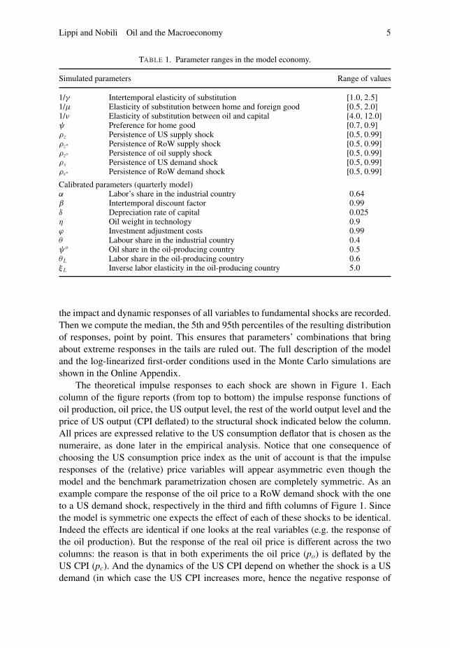
TABLE 1. Parameter ranges in the model economy.

Simulated parameters Range of values

1/γ Intertemporal elasticity of substitution [1.0, 2.5]1/μ Elasticity of substitution between home and foreign good [0.5, 2.0]1/ν Elasticity of substitution between oil and capital [4.0, 12.0]ψ Preference for home good [0.7, 0.9]ρz Persistence of US supply shock [0.5, 0.99]ρz∗ Persistence of RoW supply shock [0.5, 0.99]ρzo Persistence of oil supply shock [0.5, 0.99]ρs Persistence of US demand shock [0.5, 0.99]ρs∗ Persistence of RoW demand shock [0.5, 0.99]

Calibrated parameters (quarterly model)α Labor’s share in the industrial country 0.64β Intertemporal discount factor 0.99δ Depreciation rate of capital 0.025η Oil weight in technology 0.9ϕ Investment adjustment costs 0.99θ Labour share in the industrial country 0.4ψo Oil share in the oil-producing country 0.5θL Labor share in the oil-producing country 0.6ξL Inverse labor elasticity in the oil-producing country 5.0

the impact and dynamic responses of all variables to fundamental shocks are recorded.Then we compute the median, the 5th and 95th percentiles of the resulting distributionof responses, point by point. This ensures that parameters’ combinations that bringabout extreme responses in the tails are ruled out. The full description of the modeland the log-linearized first-order conditions used in the Monte Carlo simulations areshown in the Online Appendix.

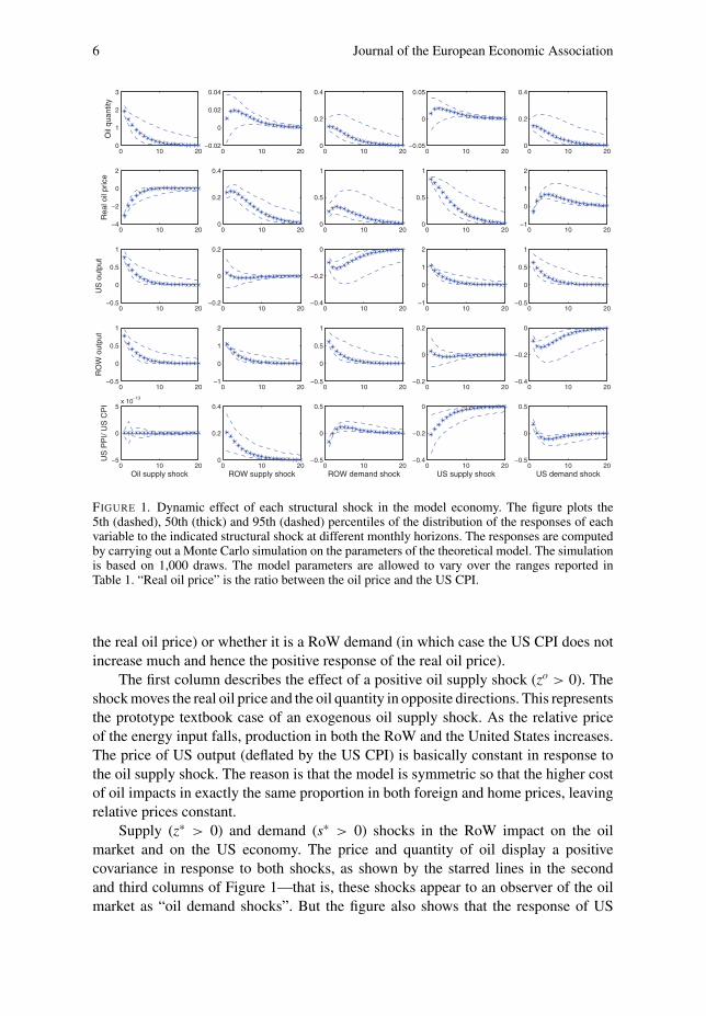
The theoretical impulse responses to each shock are shown in Figure 1. Eachcolumn of the figure reports (from top to bottom) the impulse response functions ofoil production, oil price, the US output level, the rest of the world output level and theprice of US output (CPI deflated) to the structural shock indicated below the column.All prices are expressed relative to the US consumption deflator that is chosen as thenumeraire, as done later in the empirical analysis. Notice that one consequence ofchoosing the US consumption price index as the unit of account is that the impulseresponses of the (relative) price variables will appear asymmetric even though themodel and the benchmark parametrization chosen are completely symmetric. As anexample compare the response of the oil price to a RoW demand shock with the oneto a US demand shock, respectively in the third and fifth columns of Figure 1. Sincethe model is symmetric one expects the effect of each of these shocks to be identical.Indeed the effects are identical if one looks at the real variables (e.g. the response ofthe oil production). But the response of the real oil price is different across the twocolumns: the reason is that in both experiments the oil price (po) is deflated by theUS CPI (pc). And the dynamics of the US CPI depend on whether the shock is a USdemand (in which case the US CPI increases more, hence the negative response of


FIGURE 1. Dynamic effect of each structural shock in the model economy. The figure plots the5th (dashed), 50th (thick) and 95th (dashed) percentiles of the distribution of the responses of eachvariable to the indicated structural shock at different monthly horizons. The responses are computedby carrying out a Monte Carlo simulation on the parameters of the theoretical model. The simulationis based on 1,000 draws. The model parameters are allowed to vary over the ranges reported inTable 1. “Real oil price” is the ratio between the oil price and the US CPI.

the real oil price) or whether it is a RoW demand (in which case the US CPI does notincrease much and hence the positive response of the real oil price).

The first column describes the effect of a positive oil supply shock (zo > 0). Theshock moves the real oil price and the oil quantity in opposite directions. This representsthe prototype textbook case of an exogenous oil supply shock. As the relative priceof the energy input falls, production in both the RoW and the United States increases.The price of US output (deflated by the US CPI) is basically constant in response tothe oil supply shock. The reason is that the model is symmetric so that the higher costof oil impacts in exactly the same proportion in both foreign and home prices, leavingrelative prices constant.

Supply (z∗ > 0) and demand (s∗ > 0) shocks in the RoW impact on the oilmarket and on the US economy. The price and quantity of oil display a positivecovariance in response to both shocks, as shown by the starred lines in the secondand third columns of Figure 1—that is, these shocks appear to an observer of the oilmarket as “oil demand shocks”. But the figure also shows that the response of US


production to these shocks is not the same. The difference in the response is due tothe fact that in a general equilibrium a positive RoW supply shock increases the totalamount of resources available in the economy. With perfect risk sharing, consumptiontends to increase in both countries. As the foreign and home goods are imperfectsubstitutes in consumption, the effect on US production depends on the consumptionsubstitution elasticity between home and foreign goods. If the elasticity is unitary,then the US output stays constant. When the substitution elasticity is smaller thanone, the goods are complements and US output increases after a positive RoW shock.The reverse happens for a substitution elasticity bigger than one. Now consider theeffect of a positive RoW demand shock. This increases the real cost of oil and theprice of imported foreign goods, so that the final effect on US consumption and on USproduction is an unambiguous reduction.

The fourth and fifth columns describe the effects of US shocks. A positiveproductivity shock (z > 0) raises US production and reduces its price (relative to theCPI). The ensuing increase in oil demand ultimately leads to higher real oil prices andoutput, though the latter is not robust across the different parameterizations. Finally, apositive US demand shock (s > 0) increases US production and its price (relative to theCPI). The increased demand spills over to the oil market, where production increases.

The model economy shows that the expected change of US production conditionalon an oil price increase depends on the underlying fundamental shock. For instance,while the oil price hike caused by an adverse oil supply shock is followed by a decreaseof US production, the oil price hike caused by a positive US supply shock is followedby an increase of US output. Therefore, it should not be surprising that over a longsample period the unconditional correlation between oil prices and US GDP appearstenuous, as it blurs conditional correlations with different signs. The empirical analysiswill allow us to cast light on the empirical validity of this conjecture.

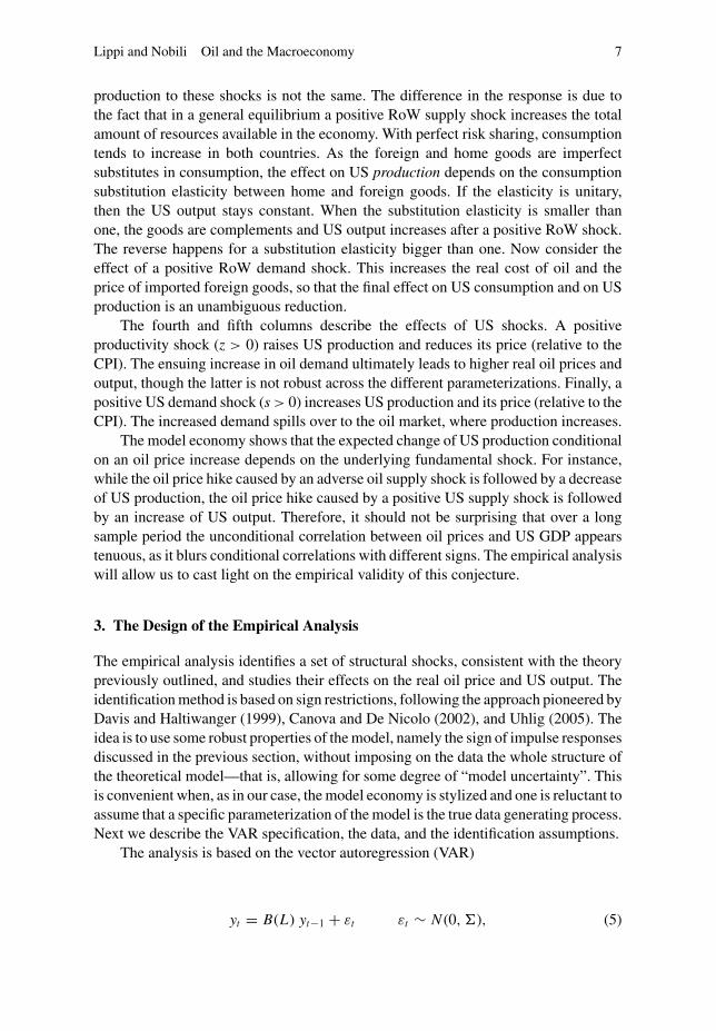
3. The Design of the Empirical Analysis

The empirical analysis identifies a set of structural shocks, consistent with the theorypreviously outlined, and studies their effects on the real oil price and US output. Theidentification method is based on sign restrictions, following the approach pioneered byDavis and Haltiwanger (1999), Canova and De Nicolo (2002), and Uhlig (2005). Theidea is to use some robust properties of the model, namely the sign of impulse responsesdiscussed in the previous section, without imposing on the data the whole structure ofthe theoretical model—that is, allowing for some degree of “model uncertainty”. Thisis convenient when, as in our case, the model economy is stylized and one is reluctant toassume that a specific parameterization of the model is the true data generating process.Next we describe the VAR specification, the data, and the identification assumptions.

The analysis is based on the vector autoregression (VAR)

yt = B(L) yt−1 + εt εt ∼ N (0, �), (5)


where B(L) is a lag polynomial of order p and yt contains five variables (all in logs)describing the United States, the RoW, and the oil market. The first two are the USindustrial production and the producer price index. Two additional variables describethe oil market: the real spot oil price and the global oil production. The fifth variableis total imports to the RoW, aiming at capturing economic activity in the RoW. Wecannot use a RoW industrial production index due to the lack of a sufficiently longtime series for output in a country group for RoW that includes China and India. InKilian (2009) the measure of global real economic activity is based on a global indexof dry cargo single-voyage freight rates (deflated by the US CPI). Increase in freightrates may be used as an indicator of cumulative global demand pressure. This measure,however, does not distinguish between increase in demand stemming from the UnitedStates and those originating in the RoW. Our results are robust to the use of Kilian’smeasure of world output instead of the RoW imports. Data description and the sourceof the variables are described in the Appendix.

Estimation of the VAR is based on monthly data spanning the period betweenJanuary 1973 and February 2009 (this uses the longest available production time seriesprovided by the International Energy Agency). The period covers all the relevantepisodes characterized by major oil price increases, including the most recent one.We complete the specification by using a lag order of two months, as suggested bythe Bayesian Information Criteria (BIC), which provides estimated residuals for thereduced-form VAR characterized by good white-noise properties. The appropriate laglength has been debated in the literature, see Hamilton and Herrera (2004) and Kilian(2009). Our results remain virtually unchanged if seven lags (as suggested by theAkaike Information Criteria) or if twelve lags are used.

The structural VAR approach sees (5) as a reduced-form representation of thestructural form

A−10 yt = A(L) yt−1 + et et ∼ N (0, I ), (6)

where A(L) is a lag polynomial of order p and the vector e includes the fivestructural innovations discussed previously, assumed to be orthogonal. Identificationof the structural shocks thus amounts to select a matrix A0 (i.e. a set ofrestrictions) that uniquely solves—up to an orthogonal transformation—for thefollowing decomposition of the estimated covariance matrix A0A′

0 = �. The jthcolumn of the identification matrix A0, aj, maps the structural innovations of thejth structural component of e into the contemporaneous vector of responses of theendogenous variables y, �0 = aj. The structural impulse responses of the endogenousvariables up to the horizon k, �k, can then be computed using the B(L) estimates fromthe reduced-form VAR, B1, B2, . . . , Bp, and the impulse vector aj.

The sign restriction approach identifies a set of structural models, the A0 ∈ A0,such that the (vectors of) impulse responses the � implied by each A0 over thefirst k horizons are consistent with the sign restrictions derived from the theory. Theapproach exploits the fact that given an arbitrary identification matrix A0 satisfyingA0A′

0 = �, any other identification matrix A0 can be expressed as the product ofA0 and an orthogonal matrix Q. The set of the theory-consistent models A0 can be


characterized as follows. For a given estimate of the reduced-form VAR, B(L) and �,take an arbitrary identification matrix A0 and compute the set of candidate structuralmodels A0 = {A0 Q | Q Q′ = I } by spanning the space of the orthogonal matrices Q.The set A0 is then obtained by removing from the set A0 the models that violate thedesired sign restrictions. The findings can then be summarized by the properties of theresulting distribution of A0 models.

In practice we also have to decide how long the sign restrictions used foridentification should hold. In this regard, Canova and Paustian (2007) show that signrestrictions imposed on the contemporaneous relationships among variables are robustto several types of model misspecification. Following this approach, we impose thesign restrictions only on impact. As several signs of the impulse responses depend onthe model parametrization, the identification restricts attention to robust features of thecontemporaneous impact responses obtained by Monte Carlo simulations. The rangesfor the parameters used in the simulations are given in Table 1. The results of thesesimulations are reported in detail in the Online Appendix.

In the empirical analysis we restrict attention to five mutually orthogonal shocks:an oil supply shock, supply and demand shocks in the RoW, and supply and demandshocks in the United States. Next we describe the identifying assumption for eachshock, consistent with the model robust properties, which are summarized in Table 2.We define as an oil supply shock one that causes the oil production and its real price(CPI deflated) to move in opposite directions, and both the RoW and the US output todecrease, as shown in the first column of Figure 1. We define a RoW supply shock asone that moves in the same direction as the RoW output, the real oil price, and the USrelative price (the response of the oil quantity and US output are left unconstrained).A positive RoW demand shock raises the oil price, the quantity of oil and the ROWoutput, while it decreases the US industrial production. US shocks are described inthe fourth and fifth columns of Figure 1. A positive shock to the US supply is one thatinduces a negative correlation between the US industrial production and its deflator andincreases the real oil price. A positive US demand shock is one that generates a positiveresponse of the oil production, the US industrial production and its deflator (relativeto the CPI), and reduces the real oil price and RoW output. The last restriction on the

TABLE 2. Sign restrictions used for identification.

Structural shocks

VAR variables Oil supply RoW supply RoW demand US supply US demand

Oil production − + +Oil pricea + + + + −US output − − + +RoW output − + + −US output pricea + − − +Notes: A “+” (or “−”) sign indicates that the impulse response of the variable in question is restricted to bepositive (negative) on impact. A blank entry indicates that no restrictions is imposed on the response.a. Price is deflated by the US CPI.


RoW output is useful because it allows us to distinguish a (negative) oil supply shockfrom a (positive) US demand shock. It is important to remark that our identificationscheme defines mutually exclusive structural shocks, thus avoiding the possibility thatwe are confusing shocks originated in the rest of the world with US-specific shocks.In this regard, Table 2 shows that a RoW supply shock cannot be confused with a USsupply shock as the US relative price variable (US CPI/PPI) responds with an oppositesign to these shocks. At the same time, a RoW demand shock cannot be confused witha US supply shock as the US output responds with opposite sign to these two shocks.Similarly, we are also able to disentangle RoW shocks from a US demand shock.Indeed, a RoW supply shock is distinguished from a US demand shock as the responseof the RoW output is opposite in sign to these two shocks; finally, a RoW demandshock is different from a US demand shock because oil production and the real priceof oil comove in response to the former, while they exhibit opposite responses in signto the latter.

4. The Estimated Effects of Structural Shocks

This section presents our estimates on the effect of the various structural shocks. Theempirical distribution for the impulse responses are derived in a Bayesian framework.As shown by Uhlig (2005) under a standard diffuse prior for (B(L), �) and a Gaussianlikelihood for the data sample, the posterior density for the reduced-form VARparameters with sign restrictions is proportional to a standard Normal–Wishart. Thusone can simply draw from the Normal–Wishart posterior for (B(L),�).

The set of theory-consistent matrices A0 is computed using the efficient algorithmproposed by Rubio-Ramirez, Waggoner, and Zha (2005). Given an estimate for (B(L),�) and one candidate identification matrix A0 (i.e. a Choleski decomposition), thealgorithm draws an arbitrary independent standard normal (n × n) matrix X and, usingthe QR decomposition of X, generates one orthogonal matrix Q. Impulse responsesare then computed using A0Q, the rotation of the initial identification matrix, andB(L). If these impulse responses do not satisfy the sign restrictions the algorithmgenerates a different draw for X. Compared with Uhlig’s procedure, this algorithmdirectly draws from a uniform distribution instead of involving a recursive column-by-column search procedure. Thus, the informativeness of the sign restriction methodis affected by the sampling uncertainty around the estimates regarding reduced-formVAR coefficients and the covariance matrix of reduced-form innovations, as well asby the model uncertainty inherent to the possible outcomes (e.g. matrices A0) that areconsistent with the set of theoretical restrictions.

Operationally we use a two-step procedure. In the first step we generate 2,000random draws from the posterior distribution of the reduced-form VAR coefficientsB(L) and the covariance matrix of disturbances �. In the second step, the procedureruns a loop. It starts by randomly selecting one draw from the posterior distributionof the reduced-form VAR and, conditionally on it, uses the QR decomposition byRubio-Ramirez, Waggoner, and Zha (2005) to find an impulse matrix satisfying the


sign restrictions. Then, it selects an alternative draw. The loop ends when 5,000identification matrices are found. By construction, each of the models in A0 generatesorthogonal structural shocks.

We notice that the number of theory-consistent models we choose to compute islarge, so that for each draw of the reduced-form VAR the simulation algorithm findsat least one identification matrix satisfying the sign restrictions. This helps us ensurethat the posterior distribution for impulse responses that we obtain does not depend ona few selected candidate draws from the reduced form.

However, we used a relatively large number of robust sign restrictions in order todisentangle the structural shocks, thus making the analysis particularly severe from acomputational viewpoint. This is necessary because, as shown by Canova and Paustian(2007), what matters for identification is the combination of the number of restrictionsand the magnitude of the variance of the shocks in the sample period considered. Inparticular, when a small number of identification restrictions is used the identificationbecomes weak and, unless, the variance of the shock is very large, results are rarelysharp.

4.1. Impulse Responses

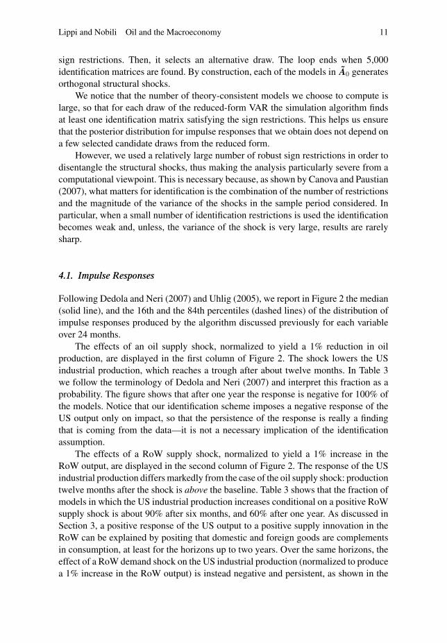
Following Dedola and Neri (2007) and Uhlig (2005), we report in Figure 2 the median(solid line), and the 16th and the 84th percentiles (dashed lines) of the distribution ofimpulse responses produced by the algorithm discussed previously for each variableover 24 months.

The effects of an oil supply shock, normalized to yield a 1% reduction in oilproduction, are displayed in the first column of Figure 2. The shock lowers the USindustrial production, which reaches a trough after about twelve months. In Table 3we follow the terminology of Dedola and Neri (2007) and interpret this fraction as aprobability. The figure shows that after one year the response is negative for 100% ofthe models. Notice that our identification scheme imposes a negative response of theUS output only on impact, so that the persistence of the response is really a findingthat is coming from the data—it is not a necessary implication of the identificationassumption.

The effects of a RoW supply shock, normalized to yield a 1% increase in theRoW output, are displayed in the second column of Figure 2. The response of the USindustrial production differs markedly from the case of the oil supply shock: productiontwelve months after the shock is above the baseline. Table 3 shows that the fraction ofmodels in which the US industrial production increases conditional on a positive RoWsupply shock is about 90% after six months, and 60% after one year. As discussed inSection 3, a positive response of the US output to a positive supply innovation in theRoW can be explained by positing that domestic and foreign goods are complementsin consumption, at least for the horizons up to two years. Over the same horizons, theeffect of a RoW demand shock on the US industrial production (normalized to producea 1% increase in the RoW output) is instead negative and persistent, as shown in the


FIGURE 2. Estimated effects of fundamental shocks. The figure plots the 16th (dashed), 50th (thick),and 84th (dashed) percentiles of the distribution of responses at each monthly horizon. The “Real oilprice” is the ratio between the oil price and the US CPI.

TABLE 3. US output response to different structural shocks.

“Probability” of a negative response of US outputa

At horizon: 1 6 12 18 24

Oil supply shock 1.00 1.00 1.00 1.00 1.00RoW supply shock 0.11 0.09 0.42 0.76 0.94RoW demand shock 1.00 1.00 1.00 1.00 1.00

a. Fraction of models A0 ∈ A0 that yield a negative response at the given horizon.

third column of Figure 2. The different effects of RoW demand and supply shocks onthe US output appear important empirically.

The fourth and fifth columns of Figure 2 illustrate the extent to which the oilmarket is affected by US shocks. A positive US aggregate supply shock raises both oilquantity and prices. A positive US aggregate demand shock raises the US productionand causes a small decrease in real oil prices (as the direct effect is to raise the price of


domestic output more than the price of the oil input) and a significant increase in theoil production.5

Our findings concerning the effect of an oil supply shock are qualitativelycomparable to those in Kilian (2009), even though the negative response of the USoutput is larger and more persistent in our estimates. The main difference concerns theeffect of the shocks in the RoW. In his analysis an expansion of the global business cycle(what Kilian labels an “aggregate demand shock”) causes a statistically nonsignificantincrease in real GDP in the first year, followed by a gradual decline which becomessignificant in the third year. Our predictions for the long run are similar, but they differover the first year, where we find that the US output response may be either positive ornegative depending on whether the fundamental innovation underlying the expansionof the global business cycle is a supply or a demand shock. Our model provides asimple explanation for the different findings: RoW demand and supply have similardynamic effects on the oil market (e.g. move price and quantity in the same direction)but they cause effects opposite in sign on the US output, at least at horizons of up toone year (see Figures 1 and 2). This suggests that by mixing together RoW supply withRoW demand shocks, one may bias the response of US output towards zero at horizonsup to one year. The variance decomposition analysis presented in the following sectioncorroborates this hypothesis since at frequencies up to one year the contribution ofthese two shocks to the variation of US production is about equal.

Altogether, the estimates show that identifying the fundamental shock underlyingthe oil price hike is key to predicting the dynamics of US output conditional onobserving an oil price increase. A higher oil price is associated with an expectedreduction of US production conditional on an adverse oil supply shock, a negativeUS demand shock, or a positive RoW demand shock. However, a higher oil priceis associated with an expected rise of US production conditional on a positive RoWsupply shock or a US supply shock.

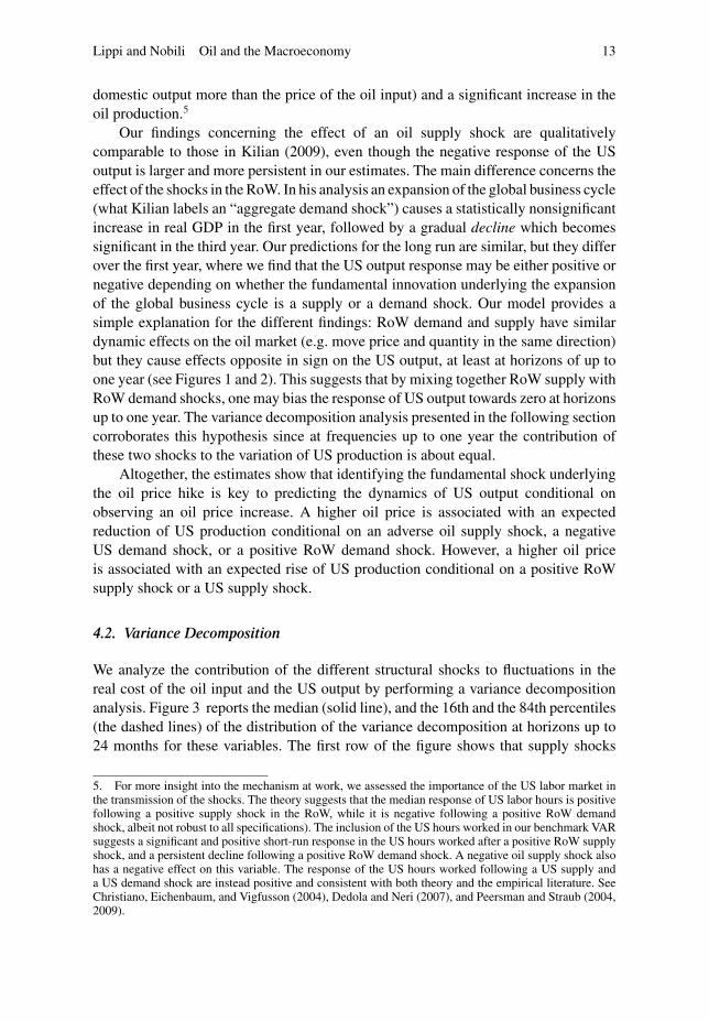
4.2. Variance Decomposition

We analyze the contribution of the different structural shocks to fluctuations in thereal cost of the oil input and the US output by performing a variance decompositionanalysis. Figure 3 reports the median (solid line), and the 16th and the 84th percentiles(the dashed lines) of the distribution of the variance decomposition at horizons up to24 months for these variables. The first row of the figure shows that supply shocks

5. For more insight into the mechanism at work, we assessed the importance of the US labor market inthe transmission of the shocks. The theory suggests that the median response of US labor hours is positivefollowing a positive supply shock in the RoW, while it is negative following a positive RoW demandshock, albeit not robust to all specifications). The inclusion of the US hours worked in our benchmark VARsuggests a significant and positive short-run response in the US hours worked after a positive RoW supplyshock, and a persistent decline following a positive RoW demand shock. A negative oil supply shock alsohas a negative effect on this variable. The response of the US hours worked following a US supply anda US demand shock are instead positive and consistent with both theory and the empirical literature. SeeChristiano, Eichenbaum, and Vigfusson (2004), Dedola and Neri (2007), and Peersman and Straub (2004,2009).


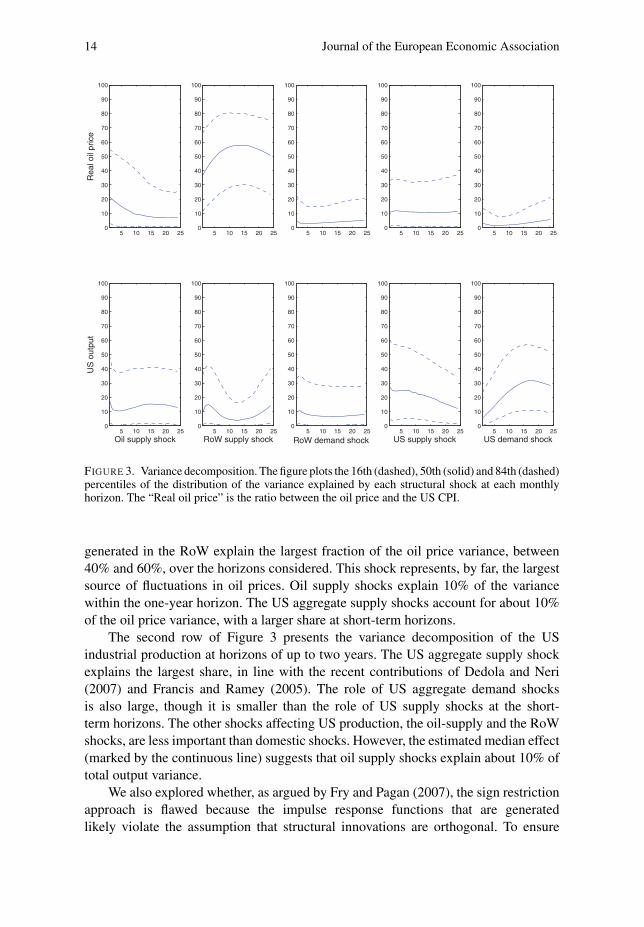
FIGURE 3. Variance decomposition. The figure plots the 16th (dashed), 50th (solid) and 84th (dashed)percentiles of the distribution of the variance explained by each structural shock at each monthlyhorizon. The “Real oil price” is the ratio between the oil price and the US CPI.

generated in the RoW explain the largest fraction of the oil price variance, between40% and 60%, over the horizons considered. This shock represents, by far, the largestsource of fluctuations in oil prices. Oil supply shocks explain 10% of the variancewithin the one-year horizon. The US aggregate supply shocks account for about 10%of the oil price variance, with a larger share at short-term horizons.

The second row of Figure 3 presents the variance decomposition of the USindustrial production at horizons of up to two years. The US aggregate supply shockexplains the largest share, in line with the recent contributions of Dedola and Neri(2007) and Francis and Ramey (2005). The role of US aggregate demand shocksis also large, though it is smaller than the role of US supply shocks at the short-term horizons. The other shocks affecting US production, the oil-supply and the RoWshocks, are less important than domestic shocks. However, the estimated median effect(marked by the continuous line) suggests that oil supply shocks explain about 10% oftotal output variance.

We also explored whether, as argued by Fry and Pagan (2007), the sign restrictionapproach is flawed because the impulse response functions that are generatedlikely violate the assumption that structural innovations are orthogonal. To ensure


orthogonality of the structural shocks we follow their suggestion and select a uniqueA0, chosen so as to minimize a minimum distance criterion from the median responses.Details on this analysis are given in the Online Appendix. The results, as measured bythe impulse responses and the variance decomposition, are similar to those producedby the median of the forecast variance posterior distribution implied by the set of A0

models.

4.3. Historical Decomposition

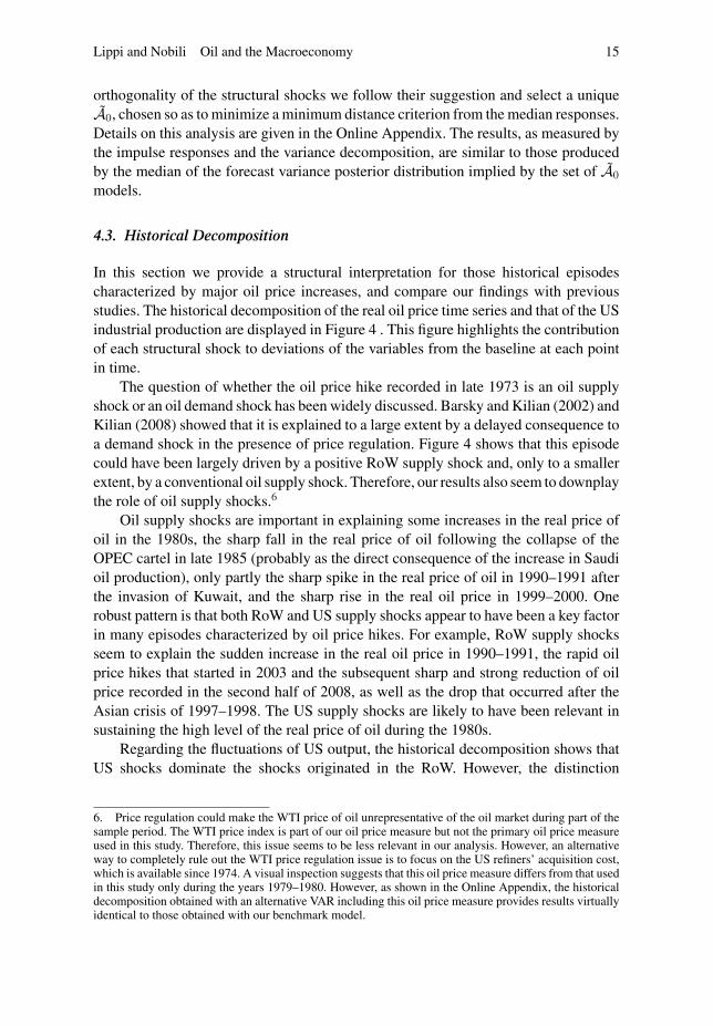
In this section we provide a structural interpretation for those historical episodescharacterized by major oil price increases, and compare our findings with previousstudies. The historical decomposition of the real oil price time series and that of the USindustrial production are displayed in Figure 4 . This figure highlights the contributionof each structural shock to deviations of the variables from the baseline at each pointin time.

The question of whether the oil price hike recorded in late 1973 is an oil supplyshock or an oil demand shock has been widely discussed. Barsky and Kilian (2002) andKilian (2008) showed that it is explained to a large extent by a delayed consequence toa demand shock in the presence of price regulation. Figure 4 shows that this episodecould have been largely driven by a positive RoW supply shock and, only to a smallerextent, by a conventional oil supply shock. Therefore, our results also seem to downplaythe role of oil supply shocks.6

Oil supply shocks are important in explaining some increases in the real price ofoil in the 1980s, the sharp fall in the real price of oil following the collapse of theOPEC cartel in late 1985 (probably as the direct consequence of the increase in Saudioil production), only partly the sharp spike in the real price of oil in 1990–1991 afterthe invasion of Kuwait, and the sharp rise in the real oil price in 1999–2000. Onerobust pattern is that both RoW and US supply shocks appear to have been a key factorin many episodes characterized by oil price hikes. For example, RoW supply shocksseem to explain the sudden increase in the real oil price in 1990–1991, the rapid oilprice hikes that started in 2003 and the subsequent sharp and strong reduction of oilprice recorded in the second half of 2008, as well as the drop that occurred after theAsian crisis of 1997–1998. The US supply shocks are likely to have been relevant insustaining the high level of the real price of oil during the 1980s.

Regarding the fluctuations of US output, the historical decomposition shows thatUS shocks dominate the shocks originated in the RoW. However, the distinction

6. Price regulation could make the WTI price of oil unrepresentative of the oil market during part of thesample period. The WTI price index is part of our oil price measure but not the primary oil price measureused in this study. Therefore, this issue seems to be less relevant in our analysis. However, an alternativeway to completely rule out the WTI price regulation issue is to focus on the US refiners’ acquisition cost,which is available since 1974. A visual inspection suggests that this oil price measure differs from that usedin this study only during the years 1979–1980. However, as shown in the Online Appendix, the historicaldecomposition obtained with an alternative VAR including this oil price measure provides results virtuallyidentical to those obtained with our benchmark model.


FIGURE 4. Historical decomposition. The thin line denotes the real oil price (or the US industrialproduction), in deviation from the baseline. The bars in each panel denote the component of theseries accounted for by each structural shock. The “Real oil price” is the ratio between the oil priceand the US CPI.


between oil supply shocks and RoW supply shocks remains relevant for theinterpretation of the effects on US output. Only oil supply shocks contributedsignificantly to subsequent US economic slowdown or recessions: this happened indeedin 1983, to some extent in the 1990/1991 episode and in 2000–2001. In contrast, oilprice hikes generated by RoW supply shocks played a negligible role in explaininghistorical episodes characterized by a fall in the US output.

5. Robustness

The robustness of the findings was tested on several dimensions.

5.1. On “Oil-Market-Specific” Demand Shocks

Kilian (2009) argues that “oil market-specific demand shocks”, namely oil price hikesrelated to concerns about future oil supply shortfalls, have a negative effect on the USeconomic activity which is more persistent than the one implied by oil supply shocksand by “aggregate demand shocks”, and that they explain many historical episodescharacterized by major oil price fluctuations, such as the sharp fall of the real oil pricein late 1985 and its sudden spike in 1990–1991. The role of these shocks has beenalso assessed empirically in Kilian and Murphy (forthcoming) and Alquist and Kilian(2010).

Our simple model economy does not allow for such “expectational shocks”. Toexplore the hypothesis that the estimates described in Figure 2 may also reflect theoil-market-specific demand shocks, we abandon (temporarily) the internal consistencyof our model economy and consider the following modification of our benchmarkVAR model. We replace the RoW demand shock with an oil-market-specific demandshock, whose identification scheme is presented in Table 4 below. In this scheme, theoil-market-specific demand shock is different from the RoW demand shock becausethe RoW output is assumed to respond negatively, rather than positively, to a positive

TABLE 4. Sign restrictions with “oil-market-specific” demand shock.

Structural shocks

oil supply RoW supply oil-market-specific US supply US demandVAR variables shock shock demand shock demand shock shock

Oil production − + +Oil pricea + + + + −US output − − + +RoW output − + − −US output pricea + − +Notes: A “+” (or “−”) sign indicates that the impulse response of the variable in question is restricted to bepositive (negative) on impact. A blank entry indicates that no restrictions is imposed on the response.a. Price is deflated by the US CPI.


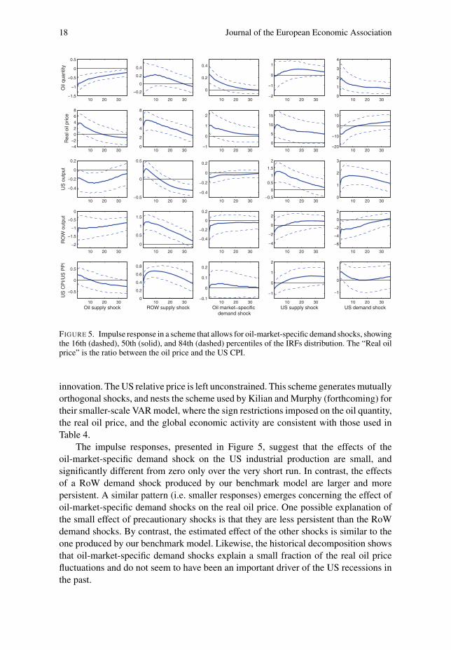
FIGURE 5. Impulse response in a scheme that allows for oil-market-specific demand shocks, showingthe 16th (dashed), 50th (solid), and 84th (dashed) percentiles of the IRFs distribution. The “Real oilprice” is the ratio between the oil price and the US CPI.

innovation. The US relative price is left unconstrained. This scheme generates mutuallyorthogonal shocks, and nests the scheme used by Kilian and Murphy (forthcoming) fortheir smaller-scale VAR model, where the sign restrictions imposed on the oil quantity,the real oil price, and the global economic activity are consistent with those used inTable 4.

The impulse responses, presented in Figure 5, suggest that the effects of theoil-market-specific demand shock on the US industrial production are small, andsignificantly different from zero only over the very short run. In contrast, the effectsof a RoW demand shock produced by our benchmark model are larger and morepersistent. A similar pattern (i.e. smaller responses) emerges concerning the effect ofoil-market-specific demand shocks on the real oil price. One possible explanation ofthe small effect of precautionary shocks is that they are less persistent than the RoWdemand shocks. By contrast, the estimated effect of the other shocks is similar to theone produced by our benchmark model. Likewise, the historical decomposition showsthat oil-market-specific demand shocks explain a small fraction of the real oil pricefluctuations and do not seem to have been an important driver of the US recessions inthe past.


TABLE 5. Median identification matrix produced by the benchmark model.

Structural shocks

Oil supply RoW supply RoW demand US supply US demandVAR variables shock shock shock shock shock

Oil production –0.0032 0.0013 0.0089 0.0007 0.0105Oil pricea 0.0411 0.0511 0.0192 0.0287 –0.0140US output –0.0028 0.0020 –0.0021 0.0036 0.0015RoW output –0.0126 0.0124 0.0050 –0.0078 –0.0075US output pricea 0.0024 0.0051 –0.0012 –0.0024 0.0015Elasticity of oil

quantity to oilprice

–0.0779 0.0254 0.4635 0.0244 –0.7500

The values are computed as the median of all matrices satisfying the sign restrictions.

One simple explanation of the difference with Kilian (2009) findings is that theshock that he labels “oil-market specific” is capturing the effects of a RoW aggregatedemand shock. Indeed, a positive oil-market-specific demand shock generates anincrease in the real price of oil, a positive short-run response of global output, albeitsmall, and a negative response of the US real GDP. This is fully consistent with theeffects of a RoW aggregate demand shock, see Table 2. Moreover, as pointed out alsoby Kilian and Murphy (forthcoming), some features of the oil-market-specific shockare “mildly implausible”: a positive oil-market-specific demand shock should have anegative effect on both the global output and the US real GDP. But in the data theoutput response of the US and the RoW is different. By contrast, these effects areconsistent with our identified RoW demand shock, which also generates an increasein the real oil price, a positive effect on the RoW output, and a negative effect on theUS output.

5.2. On the Estimated Elasticity Of Oil Supply Curve

Kilian and Murphy (forthcoming) warn about the adoption of the sign restrictionapproach when applied to empirical studies for the oil market. In particular, they arguethat the use of the median to report the impulse response functions may be inconsistentwith desirable economic features, such as a rather small price elasticity of the oil supply(Kilian 2009; Hamilton 2009), thus raising concerns about the estimated effects on theother variables of interest in the VAR.7

Table 5 reports the identification matrix obtained with the median estimates ofour empirical analysis. We find it interesting that our median estimate for the price

7. Kilian and Murphy (forthcoming) showed that the elasticity of the oil supply curve to an aggregatedemand shock generated with the sign restriction approach is 1.89. They suggest combining sign restrictionswith empirically plausible bounds on the magnitude of the short-run oil supply elasticity. The boundimposed to these fundamental structural parameters is 0.0257, derived by considering the changes in thecrude oil production and in the real oil price that occurred during a single particular episode (the outbreakof the Persian Gulf War on August 1990).


elasticity of the oil supply following a RoW supply or a US supply shock is veryclose to the bound discussed by Kilian (2009), around 3%. Therefore, for those shocksthat explain the bulk of fluctuations, as discussed in Section 4.2, our identificationscheme does not seem to generate economically implausible estimated elasticities ofthe oil supply curve, at least judging by the criterion proposed by Kilian and Murphy(forthcoming).

The estimated oil supply elasticity to a RoW demand shock is instead about0.5, which is still much smaller than the high value of 1.89 found by Kilian andMurphy (forthcoming). While it is hard to assess whether this computed elasticity iseconomically plausible, to further our analysis we estimated the model by relaxing theassumption of a positive response of the oil quantity when identifying a RoW demand(or a US demand) shock. Notice that Table 2 shows that relaxing these restrictionsdoes not impede the identification of the shocks, which remain mutually exclusive.We thus estimate the same benchmark VAR model without constraining the impactresponse of the oil quantity following a RoW and a US demand shock. The estimatedprice elasticity of the oil supply remain identical for both the RoW supply and the USsupply shock; instead, the price elasticity of the oil supply following a RoW demandshock becomes nonsignificant. The main results of our paper remain unchanged (moredetails are in the Online Appendix). In particular, following a RoW demand shock,the increase in the real oil price becomes slightly smaller and less persistent, whilethe response of US output is remarkably similar to that obtained with the benchmarkidentification scheme.

We conclude that the sign restrictions we imposed in our benchmark identificationscheme on oil production do not seem to be crucial for the assessment of themedian responses on the variables of interest, notably the US output. The impact signrestrictions imposed on the other variables are instead more important for a reliableidentification of the shocks and for the assessment of their effects on the US output.

5.3. Other Econometric Issues

We briefly summarize the findings of a few other issues that have been explored. As theOnline Appendix shows, first, we compare the impulse responses of our benchmarkmodel with those stemming from the same VAR but using a scheme that identifies onlythree, as opposed to five, structural shocks. This corresponds to identifying A0 matricesusing the restrictions of the first three columns only of Table 2. The response of the USoutput to the different oil shocks is qualitatively the same. However, the effect of an oilsupply shock is roughly one-half in magnitude, while that of a RoW demand shock issmaller by one-third on impact. These results corroborate the importance of identifyingsimultaneously both US-specific shocks, as well as shocks originating outside the USeconomy, in order to avoid biased estimated response of the US industrial productionto structural shocks moving the real price of oil.

Second, we re-estimated the VAR where we use first-difference of the non-stationary variables, instead of including the linear trend. Global crude oil production is


expressed in log first-differences while the US industrial production, the RoW output,and the US relative price measure are expressed in growth rates. The estimated impulseresponses suggest that our results are qualitatively robust to the way we handle thenon-stationarity of the variables. Interestingly, the variance decomposition analysis isalso consistent with the one previously discussed.

Third, we investigated whether our results for the US industrial production can begeneralized to a broader measure of the US economic activity. The use of industrialproduction might have the downside that it is not necessarily the variable policymakersare most interested in and it is a measure of gross output rather than does value added.This could matter for the comparison with Kilian (2009) to the extent that gross outputresponds differently to oil price shocks than value added. To this end, we repeat ouranalysis by replacing the US industrial production with the monthly Chicago FedNational Activity Index (CFNAI), which is commonly recognized to be a coincidentindicator of the US national economic activity. Impulse responses suggest results verysimilar to those obtained with the US industrial production index.

Finally, we explored the consequence of applying the sign restrictions on the USrelative prices in later periods than the impact one. This might be important if pricesadjust slowly to shocks. In particular, we check the results obtained by imposing signrestrictions on the US relative prices after three and six months, leaving unconstrainedthe response in the previous periods. Results are very similar to those obtained withthe benchmark identification scheme. An exception is a stronger response of the USoutput following a RoW demand shock.

6. Concluding Remarks

We presented a model, adapted from Backus and Crucini (2000), where the cost ofthe oil input and US production respond to demand and supply shocks generateddomestically and in the world economy. We use several robust predictions of thetheoretical model to identify the fundamental shocks underlying observed time seriesfrom the oil market, the US economy, and the global business cycle.

We summarize the main findings of the paper as follows. First, the variancedecomposition analysis shows that about one-half of the (real) oil price fluctuationsare explained by shocks to the RoW business cycle. The oil price is also shown torespond to shocks originated in the US economy, which explain a fraction of variancecomparable of the one stemming from canonical oil supply shocks. This finding isnovel and highlights the importance of not assuming that oil market variables arepredetermined with respect to the US economy. The reverse causality, from aggregatedemand and supply shocks to the oil price, supports the effort in building models wherethe oil price, like all other prices, responds to business cycle shocks (see the recentpapers by Bodenstein, Erceg, and Guerrieri (2007) and Nakov and Pescatori (2010b).

Second, the estimates qualify the results in Kilian (2009) by showing that not alloil demand shocks are alike. In particular, positive innovations to RoW-demand orRoW-supply shocks increase global output and the real price of oil, but have opposite


implications concerning the US industrial production at horizons of up to one year.Therefore, shocks that appear as “oil-demand” may have very different implications forthe US depending on whether they are originated in the US or in the RoW. The theoryoffers a simple explanation for this finding: a supply shock in the rest of the worldincreases world income and consumption and, provided the substitution elasticitybetween home and foreign goods is small enough, it also increases the production ofUS goods. Instead, an aggregate demand shock in the RoW does not increase the worldincome, it increases the cost of US imported goods, and hence reduces US demandand production.

Third, the traditional view on the effects of oil supply shocks is solid: the estimatessuggest that the impact of a negative oil supply shock on US production is negative,large, and highly persistent. However, the role of oil supply shocks with respect toUS output fluctuations is limited, explaining about 10% of the total variance. This isdue to the fact that the variance of these shocks is small compared to the variance ofdomestic aggregate demand and supply shocks.

These findings offer a simple interpretation of the small and unstable correlationbetween oil prices and the US economic activity documented in, for example, Hamilton(2008). Depending on the nature of the fundamental shock, a negative correlationemerges in periods when oil supply shocks or global demand shocks occur, while apositive correlation emerges in periods of supply shocks in the rest of the industrialworld or in the United States. The unconditional correlation between oil prices andUS production over a long sample period is tenuous because it blends conditionalcorrelations with different signs. Our explanation does not appeal to “structuralchange”. In this sense it is different from the hypothesis recently put forth by Blanchardand Gali (2010) who maintain the assumption that oil prices are predetermined to theUS economy, and argue that the smaller effect of oil shocks on the US economy inrecent years can be ascribed to structural changes, such as changes in real and nominalwage rigidity, or the energy share of production.

We see several interesting questions for future research. For instance, the simplestructural model we considered abstracts from other mechanisms that might haveaffected oil prices, such as “speculation” or “precautionary” oil shocks (Alquist andKilian 2010; Dvir and Rogoff 2009). Our tentative analysis on the role of these shocks,in Section 5.1, seemed to downplay their importance. But we think that a more rigorousanalysis is necessary to precisely identify these shocks and their effects.

Appendix: Data Description and Source of the Variables

US Output. US Industrial Production Index (index 2007 = 100), seasonally adjusted,measured in logarithms. Source: Board of Governors of the Federal Reserve System.

US CPI. US Consumer Price Index for All Urban Consumers (index 1982–1984=100), all items, seasonally adjusted. Source: US Department of Labor, Bureau ofLabor Statistics.


US Relative Prices. US Producer Price Index (index 1982=100), all commodities,not seasonally adjusted. It is expressed in real terms (e.g. deflated by the US ConsumerPrice Index) and measured in logarithms. Source: authors’ calculation based on datafrom US Department of Labor, Bureau of Labor Statistics.

Oil Quantity. Global oil production in barrels per day, measured in logarithms.Source: International Energy Agency.

Oil Price. The nominal spot oil price is the simple arithmetic average of the UKBrent, Dubai Fateh, and West Texas Intermediate spot prices, in dollars per barrel. Itis expressed in real terms (e.g. deflated by the US CPI) and measured in logarithms.Source: authors’ calculations based on data from International Monetary Fund (IMF)and US Department of Labor, Bureau of Labor Statistics.

RoW Output. Global exports to World (IMF code: WDI7D0WDA) net of globalimports from United States (IMF code: WDI7D1USA) and global imports fromoil-exporting countries (IMF code: WDI7D1OPA), seasonally adjusted by TRAMO-SEATS. It is expressed in real terms (e.g. deflated by the US CPI) and measuredin logarithms. Source: authors’ calculations based on data from Thomson ReutersDatastream and US Department of Labor, Bureau of Labor Statistics.

CFNAI Index. Chicago Fed National Activity Index. Source: Federal Reserve Bankof Chicago.

Kilian’s Measure of World Output. Global index of dry cargo single-voyage freightrates, deflated by the US Consumer Price Index, expressed in deviation from a long-runlinear trend. Source: http://www-personal.umich.edu/lkilian/rea.txt.

US Refiners’ Acquisition Cost of Crude Oil. US crude oil composite (domestic andimported) acquisition cost by refiners, expressed in dollars per barrel and measured bylogarithms. Source: US Energy Information Administration.

Supporting Information

Additional Supporting Information may be found in the online version of this article:

Appendix S1. Fry and Pagan’s critique (pdf file)Appendix S2. Data sets and software for replication of the analysis in the paper (zipfile)

Please note: Blackwell Publishing are not responsible for the content or functionalityof any supporting materials supplied by the authors. Any queries (other than missingmaterial) should be directed to the corresponding author for the article.


References

Alquist, Ron, and Lutz Kilian (2010). “What Do We Learn from the Price of Crude Oil Futures?”Journal of Applied Econometrics, 25, 539–573.

Anzuini, Alessio, Patrizio Pagano, and Massimiliano Pisani (2007). “Oil Supply Newsin a VAR: Information from Financial Markets.” Temi di Discussione (EconomicWorking Papers) No. 632, Economic Research Dept, Bank of Italy. Available athttp://ideas.repec.org/p/bdi/wptemi/td_632_07.html.

Backus, David K., and Mario J. Crucini (2000). “Oil Prices and the Terms of Trade.” Journal ofInternational Economics, 50, 185–213.

Backus, David K., Patrick J. Kehoe, and Finn E. Kydland (1994). “Dynamics of the Trade Balanceand the Terms of Trade: The J-Curve?” American Economic Review, 84(1), 84–103.

Barsky, Robert B., and Lutz Kilian (2002). “Do We Really Know that Oil Caused the GreatStagflation? A Monetary Alternative.” In NBER Macroeconomics Annual 2001, edited by B.Bernanke and K. Rogoff. MIT Press, pp. 137–183.

Barsky, Robert B., and Lutz Kilian (2004). “Oil and the Macroeconomy since the 1970s.” Journalof Economic Perspectives, 18(4), 115–134.

Baumeister, Christiane, and Gert Peersman (2008). “Time-Varying Effects of Oil Supply Shocks onthe US Economy.” Working Paper No. 08/515, Ghent University.

Baxter, Marianne, and Mario J. Crucini (1993). “Explaining Saving Investment Correlations.”American Economic Review, 83(3), 416–436.

Blanchard, Olivier, and Jordi Gali (2010). “Labor Markets and Monetary Policy: A New KeynesianModel with Unemployment.” American Economic Journal: Macroeconomics, 2, 1–30.

Blanchard, Olivier J., and Marianna Riggi (2009). “Why are the 2000s so Different from the 1970s?A Structural Interpretation of Changes in the Macroeconomic Effects of Oil Prices.” NBERWorking Paper No. 15467. Available at http://ideas.repec.org/p/nbr/nberwo/15467.html.

Bodenstein, Martin, Christopher J. Erceg, and Luca Guerrieri (2007). “Oil Shocks and ExternalAdjustment.” FRB International Finance Discussion Paper No. 897.

Canova, Fabio, and Gianni De Nicolo (2002). “Monetary Disturbances Matter for BusinessFluctuations in the G-7.” Journal of Monetary Economics, 49, 1131–1159.

Canova, Fabio, and Matthias Paustian (2007). “Measurement with Some Theory: Using Signrestrictions to Evaluate Business Cycle Models.” Working paper, CREI.

Christiano, Lawrence J., Martin Eichenbaum, and Robert Vigfusson (2004). “The Response ofHours to a Technology Shock: Evidence Based on Direct Measures of Technology.” Journal ofthe European Economic Association, 2, 381–395.

Cunado, Juncal, and Fernando Perez de Gracia (2003). “Do oil price shocks matter? Evidence forsome European countries.” Energy Economics, 25, 137–154.

Davis, Steven J., and John Haltiwanger (1999). “On the Driving Forces behind Cyclical Movementsin Employment and Job Reallocation.” American Economic Review, 89(5), 1234–1258.

Dedola, Luca, and Stefano Neri (2007). “What Does a Technology Shock do? A VAR Analysis withModel-Based Sign Restrictions.” Journal of Monetary Economics, 54, 512–549.

Dvir, Eyal, and Kenneth S. Rogoff (2009). “Three Epochs of Oil.” NBER Working Paper No. 14927.Available at http://ideas.repec.org/p/nbr/nberwo/14927.html.

Edelstein, Paul and Lutz Kilian (2009). “How Sensitive are Consumer Expenditures to Retail EnergyPrices?” Journal of Monetary Economics, 56, 766–779.

Francis, Neville, and Valerie A. Ramey (2005). “Is the Technology-Driven Real BusinessCycle Hypothesis Dead? Shocks and Aggregate Fluctuations Revisited.” Journal of MonetaryEconomics, 52, 1379–1399.

Fry, Renee, and Adrian Pagan (2007). “Some Issues in Using Sign Restrictions for IdentifyingStructural VARs.” NCER Working Paper No. 14.

Hamilton, James D. (1983). “Oil and the Macroeconomy since World War II.” Journal of PoliticalEconomy, 91, 228–248.


Hamilton, James D. (2008). “Oil and the Macroeconomy.” In The New Palgrave Dictionary ofEconomics, 2nd ed, edited by S. Durlauf and L. Blume. Palgrave MacMillan.

Hamilton, James D. (2009). “Causes and Consequences of the Oil Shock of 2007–08.” NBERWorking Paper No. 15002. Available at http://ideas.repec.org/p/nbr/nberwo/15002.html.

Hamilton, James D, and Ana Maria Herrera (2004). “Oil Shocks and Aggregate MacroeconomicBehavior: The Role of Monetary Policy: Comment.” Journal of Money, Credit and Banking, 36,265–86.

Hooker, Mark A. (1996). “What Happened to the Oil Price–Macroeconomy Relationship?” Journalof Monetary Economics, 38, 195–213.

Jimenez-Rodriguez, Rebeca, and Marcelo Sanchez (2005). “Oil Price Shocks and Real GDP Growth:Empirical Evidence for some OECD Countries.” Applied Economics, 37, 201–228.

Kilian, Lutz (2008). “Exogenous Oil Supply Shocks: How Big Are They and How Much Do TheyMatter for the U.S. Economy?” The Review of Economics and Statistics, 90, 216–240.

Kilian, Lutz (2009). “Not All Oil Price Shocks Are Alike: Disentangling Demand and Supply Shocksin the Crude Oil Market.” American Economic Review, 99(3), 1053–1069.

Kilian, Lutz, and Dan Murphy (forthcoming). “Why Agnostic Sign Restrictions Are Not Enough:Understanding the Dynamics of Oil Market VAR Models.” Journal of the European EconomicAssociation.

Kilian, Lutz, and Clara Vega (2008). “Do Energy Prices Respond to U.S. Macroeconomic News?A Test of the Hypothesis of Predetermined Energy Prices.” CEPR Discussion Paper No. 7015.Available at http://ideas.repec.org/p/cpr/ceprdp/7015.html.

Leduc, Sylvain, and Keith Sill (2004). “A Quantitative Analysis of Oil-Price Shocks, SystematicMonetary Policy, and Economic Downturns.” Journal of Monetary Economics, 51, 781–808.

Mork, Knut A., Oystein Olsen, and Hans Terje Mysen (1994). “Macroeconomic Responses to OilPrice Increases and Decreases in Seven OECD Countries.” Energy Journal, 15, 19–35.

Nakov, Anton, and Andrea Pescatori (2010a). “Monetary Policy Trade Offs with a Dominant OilProducer.” Journal of Money, Credit and Banking, 42, 1–32.

Nakov, Anton, and Andrea Pescatori (2010b). “Oil and the Great Moderation.” Economic Journal,120, 131–156.

Pagano, Patrizio, and Massimiliano Pisani (2009). “Risk-Adjusted Forecasts of Oil Prices.” The B.E.Journal of Macroeconomics, 9(1).

Pappa, Evi (2009). “The Effects Of Fiscal Shocks On Employment And The Real Wage.”International Economic Review, 50, 217–244.

Peersman, Gert, and Roland Straub (2004). “Technology Shocks and Robust Sign Restrictions in aEuro Area SVAR.” Working Paper No. 373, European Central Bank.

Peersman, Gert, and Roland Straub (2009). “Technology Shocks And Robust Sign Restrictions In AEuro Area Svar.” International Economic Review, 50, 727–750.

Rubio-Ramirez, Juan F., Daniel Waggoner, and Tao Zha (2005). “Markov Switching Structural VectorAutoregressions: Theory and Application.” Federal Reserve Bank of Atlanta Working Paper No.27.

Uhlig, Harald. (2005). “What Are the Effects of Monetary Policy on Output? Results from anAgnostic Identification Procedure.” Journal of Monetary Economics, 52, 381–419.

OIL AND THE MACROECONOMY: A QUANTITATIVE STRUCTURAL ANALYSIS

Documents

Transcript of OIL AND THE MACROECONOMY: A QUANTITATIVE STRUCTURAL ANALYSIS