Oil analysis in machine diagnostics - Oulu

U N I V E R S I TAT I S O U L U E N S I SACTAA

SCIENTIAE RERUMNATURALIUM

OULU 2006

A 458

Pekka Vähäoja

OIL ANALYSISIN MACHINE DIAGNOSTICS

FACULTY OF SCIENCE,DEPARTMENT OF CHEMISTRY, DEPARTMENT OF MECHANICAL ENGINEERING,UNIVERSITY OF OULU

ABCDEFG

UNIVERS ITY OF OULU P.O. Box 7500 F I -90014 UNIVERS ITY OF OULU F INLAND

A C T A U N I V E R S I T A T I S O U L U E N S I S

S E R I E S E D I T O R S

SCIENTIAE RERUM NATURALIUM

HUMANIORA

TECHNICA

MEDICA

SCIENTIAE RERUM SOCIALIUM

SCRIPTA ACADEMICA

OECONOMICA

EDITOR IN CHIEF

EDITORIAL SECRETARY

Professor Mikko Siponen

Professor Harri Mantila

Professor Juha Kostamovaara

Professor Olli Vuolteenaho

Senior assistant Timo Latomaa

Communications Officer Elna Stjerna

Senior Lecturer Seppo Eriksson


Publication Editor Kirsti Nurkkala

ISBN 951-42-8075-X (Paperback)ISBN 951-42-8076-8 (PDF)ISSN 0355-3191 (Print)ISSN 1796-220X (Online)

A 458

AC

TA Pekka Vähäoja

A458etukansi.fm Thursday, April 13, 2006 11:10 AM

A C T A U N I V E R S I T A T I S O U L U E N S I SA S c i e n t i a e R e r u m N a t u r a l i u m 4 5 8

PEKKA VÄHÄOJA


Academic Dissertation to be presented with the assent ofthe Faculty of Science, University of Oulu, for publicdiscussion in Raahensali (Auditorium L10), Linnanmaa,on June 9th, 2006, at 12 noon

OULUN YLIOPISTO, OULU 2006

Copyright © 2006Acta Univ. Oul. A 458, 2006

Supervised byDocent Toivo KuokkanenProfessor Sulo Lahdelma

Reviewed byProfessor Kenneth HolmbergDocent Risto Pöykiö

ISBN 951-42-8075-X (Paperback)ISBN 951-42-8076-8 (PDF) http://herkules.oulu.fi/isbn9514280768/ISSN 0355-3191 (Printed )ISSN 1796-220X (Online) http://herkules.oulu.fi/issn03553191/

Cover designRaimo Ahonen

OULU UNIVERSITY PRESSOULU 2006

Vähäoja, Pekka, Oil analysis in machine diagnosticsFaculty of Science, Department of Chemistry, University of Oulu, P.O.Box 3000, FI-90014University of Oulu, Finland, Department of Mechanical Engineering, University of Oulu, P.O.Box4200, FI-90014 University of Oulu, Finland Acta Univ. Oul. A 458, 2006Oulu, Finland

Abstract

This study concentrates on developing and tuning various oil analysis methods to meet therequirements of modern industry and environmental analytics. Oil analysis methods form a vital partof techniques used to monitor the condition of machines and may help to improve the overallequipment effectiveness value of a factory in a significant manner.Worm gears are used in various production machines, and their breakdowns may cause significantproduction losses. Wearing of these gears is relatively difficult to monitor with vibration analysis.Analysis of two indicator metals, copper and iron, may reveal wearing phenomena of worm gearseffectively, and savings can be significant.

Effective wear metal analysis requires good tools. ICP-OES with kerosene dilution is widely usedin wear metal analysis, but purchasing and using of ICP-OES is expensive. A cheaper FAAStechnique with similar pre-treatment of oil samples was tested and it proved to be useful especially inanalyzing small amounts of samples. The accuracy of FAAS was sufficient for quantitative work inmachine diagnostics and waste oil characterization. Solid debris analyses are useful in oilcontamination control as well as in detection of wearing mechanisms. Membrane filtration, opticalmicroscopy, SEM and automatic particle counting were applied in analysis of rolling and gear oils.Particle counting is an effective way to detect oil contamination, but in the studied cases even largerparticles than those detected in normal ISO classes would be informative. However, membranefiltration and optical microscopy may reveal the wearing machine element exactly. Additives provideoils with desired properties thus they should be monitored intensively. A FTIR method forquantitative analysis of fatty alcohols and fatty acid esters in machinery oils was developed duringthis work. It has already been used successfully in quantitative and qualitative analysis of machineryoil samples.

Various kinds of oils may be spilled into the soil during use and in accident situations, and theycan migrate to groundwater layers. Biodegradation of oils can remove them from the soil or watercompletely or at least diminish the amount of harmful substances. An automatic, respirometric BODOxiTop method was used to evaluate the biodegradability of various oils in water and soil media. Thebiodegradation of certain bio and mineral hydraulic oils was evaluated in groundwater, where bio oilsusually biodegraded more effectively than mineral oils. The use of oils in machines weakenedespecially the biodegradability of bio oils. Biodegradability of bio oils was also studied in standardconditions of OECD 301 F and bio oils usually biodegraded moderately good in these conditions. Thebiodegradation of forestry chain oils and wood preservative oils was evaluated in forest soils. Linseedoil biodegraded moderately, but certain experimental wood preservatives biodegraded moreeffectively. Widely used creosote oil biodegraded in a lesser degree. Rapeseed oil-based chain oilsbiodegraded more effectively than corresponding tall oil.

Keywords: additives, biodegradation, machine diagnostics, oil analysis, solid debris, wearmetals

“The difficulty in most scientific work lies in framing the questions rather than in finding the answers”

A.E. Boycott

Acknowledgements

This study was carried out in the Departments of Chemistry and Mechanical Engineering at the University of Oulu between September 2002 and December 2005.

The supervisors of my doctoral research, Docent Toivo Kuokkanen and Professor Sulo Lahdelma, are greatly acknowledged for giving me the possibility to work in the interesting field of machine diagnostics and oil analysis. Their support and help in academic and financial issues during the whole research was very important indeed. I am also grateful to all the co-authors of my articles, especially to M.Sc.(Chem.) Ilkka Välimäki, who was always ready to help in my analytical problems during the study, and to M.Sc.(Chem.) Jani Närhi, who had the persistence to finish the additive study with me. Many persons from ABB Oy Service, Mondo Minerals Oy, Outokumpu Stainless Oy, Ruukki Production (Raahe Steel Works) and Suomen Ympäristöpalvelu Oy provided valuable help and advice during the research, hence they are greatly acknowledged. Special thanks go to M.Sc.(Tech.) Aale Grekula (Outokumpu Stainless Oy), who introduced me to the world of cold rolling of stainless steel, and to Mr. Pertti Leinonen (Ruukki Production), who helped me in the crane study. I also wish to thank my colleagues and staff in the Departments of Chemistry and Mechanical Engineering.

I am grateful to the reviewers of this thesis, Professor Kenneth Holmberg (VTT Industrial Systems) and Docent Risto Pöykiö (City of Kemi, Town Planning and Building Committee, Environmental Research Division) for reading, commenting and correcting my manuscript and to Licensed Translator Keith Kosola (Translation Agency BSF) for revising the language.

Financial support was received from the National Technology Agency of Finland (TEKES) in the Prognos project and the Academy of Finland in the SUNARE project. ABB Oy Service, the Finnish Maintenance Society, Mondo Minerals Oy and Outokumpu Stainless Oy gave financial donations to the Support Foundation of the University of Oulu, which allotted grants to this study. Personal grants were also given to Pekka Vähäoja by the Tauno Tönning Foundation. All the financial support is greatly acknowledged.

Special thanks to my mother Sirpa Vähäoja for her support during my studies, from comprehensive school to the PhD level.

Oulu, April 2006 Pekka Vähäoja

Abbreviations and definitions

2D two-dimensional α Bunsen absorption coefficient a acceleration AAS atomic absorption spectroscopy AES/OES atomic/optical emission spectroscopy ANN artificial neural network ANOVA analysis of variance ASTM American Society for Testing and Materials BCF bioconcentration factor BOD/BODn biological oxygen demand (in n days) BSTFA [N, O-bis(trimethylsilyl)trifluoroacetamide] CEC Coordinating European Council C=O carbonyl group Crest factor the ratio of peak value to rms value D2 deuterium DAT digital audio tape DIBK di-isobutylketone DIN German organization for standardization DO dissolved oxygen EC electrical conductivity EDS energy dispersive spectrometer EP extreme pressure additive EPA Environmental Protection Agency of the United States FA fatty alcohol FAAS flame atomic absorption spectroscopy FAE fatty acid ester FFT fast Fourier transform

FTIR/IR Fourier transform infrared spectroscopy GC/GC-MS gas chromatography/ -mass spectrometry ICP-MS inductively coupled plasma-mass spectrometry ICP-OES inductively coupled plasma-optical emission spectroscopy ISO International Organization for Standardization Kow water/octanol distribution factor Kurtosis fourth moments normalized with respect to the standard deviation LC liquid chromatography LC50 concentration of a chemical that kills 50% of the test animals in a given

time LCA life cycle assessment or life cycle analysis LCC life cycle costs MCD magnetic chip detector MIBK methylisobutylketone MS mass spectrometry NDT non-destructive testing NF standard of AFNOR (French organization for standardization) NMR nuclear magnetic resonance spectroscopy NPG neopentylglycol NPK nitrogen-phosphorus-potassium fertilizer OECD Organisation for Economic Co-operation and Development OEE overall equipment effectiveness OH hydroxyl group p significance level p.a. pro analysis grade ppm parts per million = mg/kg PSK Organization for standardization of the Finnish process industry R gas constant R2 coefficient of determination or correlation factor RDE-OES rotary disk electrode-optical emission spectroscopy rms root-mean-square value RSD relative standard deviation SD standard deviation SEM scanning electron microscopy SFS Finnish Standards Association TAN total acid number ThOD theoretical oxygen demand TOC total organic carbon TOFA tall oil fatty acid TPM total productive maintenance

UV ultraviolet (spectroscopy) v velocity VG viscosity grade v/v, w/v, w/w volume-to-volume, weight-to-volume, weight-to-weight WGK water hazard class according to German norms x, x(n) displacement, nth time derivative of displacement XRD x-ray diffraction XRF x-ray fluorescence (spectroscopy)

List of original papers

This thesis is based on the following articles, which are referred to in the thesis by their Roman numerals:

I Vähäoja P, Lahdelma S & Kuokkanen T (2004) Condition Monitoring of Gearboxes Using Laboratory-scale Oil Analysis. In: Rao RBKN, Jones BE & Grosvenor RI (eds) Proc of the 17th Int Congress of Condition Monitoring and Diagnostic Engineering Management (COMADEM 2004), Cambridge, UK, 23rd – 25th August 2004, 104–114.

II Vähäoja P, Välimäki I, Heino K, Perämäki P & Kuokkanen T (2005) Determination of Wear Metals in Lubrication Oils: A Comparison Study of ICP-OES and FAAS. Anal Sci 21:1365–1369.

III Vähäoja P, Lahdelma S & Kuokkanen T (2005) Experiences with Different Methods for Monitoring the Quality and Composition of Solid Matter in Rolling and Gear Oils. In: Mba DU & Rao RBKN (eds) Proc of the 18th Int Congress of Condition Monitoring and Diagnostic Engineering Management (COMADEM 2005), Cranfield, UK, 31st August – 2nd September 2005, 463–473.

IV Vähäoja P, Närhi J, Kuokkanen T, Naatus O, Jalonen J & Lahdelma S (2005) An infrared spectroscopic method for quantitative analysis of fatty alcohols and fatty acid esters in machinery oils. Anal Bioanal Chem 383:305–311.

V Kuokkanen T, Vähäoja P, Välimäki I & Lauhanen R (2004) Suitability of the Respirometric BOD Oxitop Method for Determining the Biodegradability of Oils in Ground Water Using Forestry Hydraulic Oils as Model Compounds. Int J Environ Anal Chem 84:677–689.

VI Vähäoja P, Roppola K, Välimäki I & Kuokkanen T (2005) Studies of biodegradability of certain oils in forest soil as determined by the respirometric BOD OxiTop method. Int J Environ Anal Chem 85:1065–1073.

Contents

Abstract Acknowledgements Abbreviations and definitions List of original papers Contents 1 Introduction ...................................................................................................................17 2 On the methods of monitoring the condition of machinery ...........................................19

2.1 Oil analysis methods...............................................................................................19 2.1.1 Wear metal analysis .........................................................................................20 2.1.2 Solid debris analysis ........................................................................................22 2.1.3 Additive analysis .............................................................................................23

2.2 Vibration analysis methods.....................................................................................24 3 Environmental fate of lubricants ...................................................................................26

3.1 Biodegradation measurements................................................................................27 4 Aims of the study...........................................................................................................29 5 Experimental work ........................................................................................................31

5.1 Overview of the oil samples and sampling methods (I-VI) ....................................31 5.2 Wear metal analysis (I, II, III, V)............................................................................32 5.3 Solid debris analysis (III) .......................................................................................33 5.4 Additive analysis (IV).............................................................................................33 5.5 Vibration analysis (I) ..............................................................................................34 5.6 Biodegradation measurements (V, VI)....................................................................34 5.7 Other oil analysis methods (I).................................................................................36

6 Results and discussion...................................................................................................37 6.1 Oil analysis in industrial machine diagnostics (I)...................................................37

6.1.1 Case study 1 (I)................................................................................................37 6.1.2 Case study 2 (I)................................................................................................38 6.1.3 Case study 3 (I)................................................................................................40

6.2 On the wear metal analysis of oils (II)....................................................................41 6.2.1 ICP-OES method (II).......................................................................................42 6.2.2 Comparison tests of ICP-OES and FAAS (II) .................................................43

6.3 On the solid debris analysis of oils (III) .................................................................45 6.3.1 Membrane filtration (III) .................................................................................45 6.3.2 Optical microscopy (III) ..................................................................................46 6.3.3 Scanning electron microscopy (III) .................................................................48 6.3.4 Automatic particle counting (III) .....................................................................49

6.4 On the additive analysis of oils (IV).......................................................................50 6.4.1 A FTIR method for analysis of fatty alcohols and fatty acid esters (IV) .........51 6.4.2 Use of the developed FTIR method in routine analysis (IV)...........................54

6.5 Biodegradability studies of oils (V, VI) ..................................................................55 6.5.1 Biodegradability of oils in water (V)...............................................................56

6.5.1.1 Biodegradability of hydraulic oils in groundwater (V).............................56 6.5.1.2 Biodegradability of hydraulic oils in standard conditions (V)..................58

6.5.2 Biodegradability of oils in soil (VI).................................................................59 7 Conclusions ...................................................................................................................62 8 Future work ...................................................................................................................65 References Original papers

1 Introduction

Without exaggerating, it can be said that modern industry rests on a layer of lubricant which separates moving machine elements from each other. In Finland alone, over 84,500 tons of oil-based lubricants were used in 2004 (1). The condition of oil or grease used as a lubricant affects the working condition of the machine significantly. The chemical and physical properties of a lubricant have a direct effect on the lubrication situation. On the other hand, the lubricant provides secondary information about the condition of the machine. Just as a blood test can reveal several illnesses in people, a thorough oil analysis can inform about several malfunctions within a machine. If optimal lubrication conditions are not met, metal surfaces will touch each other and wearing is inevitable. Wearing in itself may cause significant expenses to industry. It has been evaluated that the total expenses due to friction and wearing could be as high as 2.7 billion euros a year in Finland and almost one third of that sum could be saved if the latest tribological knowledge were utilized (2). Without any doubt, effective use of oil analysis is one part of these cost-saving actions, hence it is included as a vital part of maintenance policies nowadays. (3)

Maintenance has developed from repairing maintenance via scheduled maintenance to predictive and even improving maintenance. Repairing maintenance meant that machines were repaired after their breakage. Scheduled maintenance added the use of a calendar to maintenance. For instance, oil changes and replacement of certain machine elements were carried out after a suitable time period or number of work hours without knowing if this was necessary or not. This kind of maintenance action is naturally justifiable if the changed oil volumes are very small, machine elements are cheap and maintenance breaks do not cause production delays. If the machine is larger or even a part of a bigger aggregate, like a paper machine, unnoticed malfunctions may cause downtime and significant production losses. Undetected malfunctions are possible if the condition of machines is not monitored intensively. Condition monitoring forms an important part of predictive maintenance and it can be carried out using e.g., oil analysis, vibration monitoring or process parameter monitoring. If condition monitoring reveals a significant constructive fault in the machine, for instance strong unbalance due to a weak base of the machine or incorrectly chosen oil type, and the machine construction or process

18

parameters are changed due to these observations, then the maintenance is improving. (4-6)

In today’s industrial production, the significance of environmental issues is continuously increasing and developing. The life cycle of industrial products should be evaluated by the manufacturer. The term “life cycle assessment” (LCA) is often used when the environmental effects of industrial products are evaluated. LCA includes e.g., production, storage, transportation, handling, use and disposal of the product and all environmental effects therein. (7) On the other hand, if the costs of certain products are evaluated, life cycle cost (LCC) terminology is used (4). Oil analysis includes quite a big portion of the total LCA and LCC of lubricating oils, namely use, disposal and possible recycling or reuse. If oil analysis is used for condition monitoring of oils and machines during use of the oils, it will be able to diminish the total life cycle costs and improve the efficiency of whole production lines (8). Oil changes or top-ups can be made based on analysis results instead of a calendar, hence diminishing the amount of waste oils and the need for new oils. Oil analysis can also help in determining the condition of machines and in predicting possible malfunctions before catastrophic failures occur, thereby decreasing repair costs and preventing production losses. It should also be noted that a properly working machine usually consumes less energy than a faulty one. The environmental effects of different oils can also be evaluated with the help of oil analysis, like the impact of oils on nature after their useful lifetime.

Oil manufacturers develop their products continuously in order to meet the requirements of modern industry. Several analysis laboratories and maintenance enterprises solve problems of lubrication, which include a wide area extending from lubrication of a single machine to development of maintenance programs for entire plants or companies. International organizations at the head of ASTM, ISO and OECD, have developed a great number of standards for oil analysis. In addition to that, national organizations, oil manufacturers or single enterprises may have oil analysis standards of their own. Nevertheless, new problems still arise and oil analysis strategies and new analysis methods developed just for certain targets are required and will also be required in the future. This dictates the justification for this and various other studies related to the vast area of oil analysis.

2 On the methods of monitoring the condition of machinery

A vast and diverse group of different methods for monitoring the condition of machines has been presented in the literature during the past few decades. These methods can be roughly divided into four groups:

− Methods for analyzing machinery oils or greases (6, 9) − Methods for analyzing machine vibrations, e.g., vibration analysis (5, 10-11) or shock

pulse method (12) − Non-destructive testing methods (NDT) like acoustic emission (13-14), thermography

(15) or ultrasound (15) − Simple following of process parameters like temperatures, pressures, flow velocities,

loadings or torques (5)

This literature survey concentrates on the most important oil analysis methods as well as on vibration analysis.

2.1 Oil analysis methods

Oil analysis methods can be divided into laboratory-scale (off-line) or continuously working (on-line/in-line) methods. On-line and in-line methods can be used to determine, for instance particle quantities in oils, water content and general oil condition, like oil degradation, based on, e.g., IR spectroscopy or electrical conductivity (16-19). On the other hand, on-line methods can be used to collect wear particles by means of magnetic chip detectors (MCD) (20). Deeper inspection of the wear particles can then be carried out with microscopic methods. On-line instruments are situated in oil circulation systems and a part of the oil circulates through the measuring device. If the device is assembled in-line, then the whole oil volume will go through the measurement system. Off-line analyses require taking a representative oil sample. (6, 16) Despite the constantly growing significance of the on-line oil condition monitoring methods, in this study, the focus is especially on laboratory-scale, off-line oil analysis methods. The current literature related to wear metal analysis, solid debris analysis and additive analysis of oils is reviewed briefly.

20

2.1.1 Wear metal analysis

Increased metal concentrations in oils may tell the maintenance personnel about wearing of machine elements or oil contamination with other oils, process chemicals or airborne dust. On the other hand, a decrease in concentrations of various additive metals can be detected for top-up purposes. Techniques used for wear metal analysis are numerous, for example, atomic absorption spectroscopy (AAS), atomic/optical emission spectroscopy (AES/OES), mass spectrometry (MS), X-ray fluorescence spectroscopy (XRF), ferrography and magnetic chip detectors (5-6, 9, 16). Spectroscopic methods usually require pre-treatment of oil samples before analysis, whereas instruments based on magnetism allow analysis to be carried out directly from the oil. Nevertheless, spectroscopic techniques are more versatile than methods based on ferromagnetism. Spectroscopic methods can be used in determinations of most metals and even with some non-metals, depending on the application.

In atomic spectroscopic methods the sample often first has to be nebulized into an excitation source, which atomizes and often also ionizes the elements of the sample. In the AAS method a light with the characteristic wavelength of the determined metal is emitted from a hollow cathode lamp and the light is absorbed by the metal atoms. The degree of absorption is detected. In OES techniques the metal atoms and/or ions are excited with the thermal energy of the excitation source. When the excitation state dies, an element-specific emission spectrum is produced. With the selection and isolation of a certain emission line, the concentration of the metal can be determined. (6, 21-22).

The literature presents several pre-treatment methods which are employed when determining metals in oils using AAS and OES methods. A common way is to use organic solvents to dissolve and dilute oils and to nebulize the oil/solvent mixture as such to the atomizer unit of the spectrometer used. Various solvents have been proposed, depending on the technique used. MIBK, DIBK, alcohols, xylene and naphtolite, among others, have been used with FAAS. Xylene and kerosene are the usual solvents with the ICP-OES technique. Dilution with organic solvents is a very rapid pre-treatment method and as such very suitable for quick check-ups of metal concentrations. It is extremely useful when metal atoms are attached to organic molecules, like in many additive substances or in metal soaps, or when the solid metal particles are mainly small in size. (23-29) The obvious drawback of the dilution method is that organic solvents do not dissolve large solid particles. These particles will not be atomized perfectly in absorption or emission spectrometric methods. In addition, very large particles are not necessary nebulized to the atomizer, but are removed to waste. The size limit for 100% atomization depends on the technique used, being the smallest for FAAS (30) and the biggest for RDE-OES (31-32). Because instrumental factors affect the limit value significantly, the literature proposes different limit values even for similar methods. But, 10 µm could be considered some kind of a rough maximum limit (29-35). The sensitivity of atomization decreases in all methods after this limit. The amount of small particles can also be significant in certain situations (29), hence the use of organic solvents as a pre-treatment method is justifiable also in wear metal analysis. The size distribution of the wear particles has no influence on the atomization efficiency if acid digested oil samples are used. The most common ways of digesting oil samples are wet digestion with different

21

acid mixtures in refluxing conditions or microwave-assisted acid digestion (25, 36-38). Dry ashing has also been used in some studies, but it is possible that easily volatile metals volatilize during the sample treatment (39-40). One popular pre-treatment method is to use microemulsions, which means mixing the oil with water and surfactants. The drawbacks of this pre-treatment method are problems with the stability of the emulsion, difficult preparation of standards and the same problem with the nebulization/atomization efficiency of large solid particles as with the use of organic solvents. However, it should be noted that adding acid to emulsified samples will dissolve the solid metal particles and improve the accuracy of the determination. (41-46)

FAAS is relatively inexpensive to purchase and use, and its routine operation is quite simple. On the other hand, sample consumption of the FAAS instrument is high, its linear determination range is narrow, determining of refractory elements is difficult and chemical interferences are possible. Only one element at a time can be determined with the FAAS instrument. Some ICP-OES and RDE-OES instruments offer a possibility to simultaneously measure almost all metals and some non-metals. These methods are almost free of chemical interference and possible spectral interferences and matrix effects can be minimized with careful planning of the measurement. RDE-OES instruments do not necessarily require any sample treatment and measurements are cheap to carry out. The drawbacks of ICP-OES are higher purchasing and use expenses than with FAAS or RDE-OES, and expertise is often required. One difficulty with RDE-OES is the strong influence of changes in instrumental factors on the results. (6, 21-22, 32) The detection limits of both atomic absorption and emission spectrometric techniques are very sufficient for condition monitoring purposes, but if even lower detection limits are required, ICP-MS can be applied (47-48). However, ICP-MS is very expensive to purchase and use, and matrix effects in the form of several molecular ions formed in the plasma can be difficult to remove (21-22).

In the XRF instrument each atom emits radiation in the X-ray region after stimulation. The detection system can measure the amount of metal atoms in the sample by determining the amount of X-ray energy produced by the atoms at their characteristic wavelengths. The XRF technique has been used successfully to determine additive metals and wear metals in oil samples, as well as wear metals in lubricant filters. Lighter metals (like magnesium and aluminum) can not be analyzed with XRF, and matrix effects can sometimes be difficult to remove. (6, 49-51) X-ray related technologies can also be used to analyze non-metallic particles in oils by means of X-ray diffraction (52).

Ferrographs are divided into direct reading types and analytical ferrographs. A direct reading ferrograph determines the concentration of ferromagnetic particles above and below 5 µm based on an optical measurement. In analytical ferrography metal particles in the oil are precipitated on a specific slide, which is then studied under a microscope. Particle types, concentrations, sizes and morphologies can be determined. Ferrographic analyzers can also be used in on-line measurements of wear debris (6, 16, 53-57). Magnetic chip detectors can also be used to collect ferrous particles. The easiest application is a simple plug routinely checked visually by maintenance personnel. Morphological analysis of the collected ferrous wear debris can be carried out with microscopic methods (20).

22

2.1.2 Solid debris analysis

Metallic solid debris in oils can originate from machine elements due to wearing. Filters, seals and other non-metallic machine parts can introduce non-metallic solid debris into oil. Severe oxidation of oil can produce solid sludge with carbon deposits. Contamination with process chemicals and environmental dust can increase the amount of solid particles in oils. (5-6, 16) The concentration of metallic solid debris can be naturally monitored with the techniques presented in Chapter 2.1.1. This chapter concentrates mostly on automatic particle counters and certain microscopic methods.

Automatic particle counting is a commonly used method for monitoring the cleanliness of hydraulic oils in particular. Automatic particle counters can be divided into three classes, as presented by Toms (6): methods based on light extinction, flow decay and mesh obscuration. Methods based on light extinction are commonly used in commercial instruments (17, 58-59) because their measurement range is wider than with instruments based on the pressure difference before and after the filters of the instrument. Particle counters based on light extinction may have problems with highly viscous and dark-colored oils and with high particle quantities. In addition, air bubbles and water introduce bias to the determined results. Air can be removed in some instruments and water is also harmful to the lubrication system, hence the detection of water can be seen as a good property, depending on the requirements. Commercial instruments are available as laboratory, portable and on-line devices. (6, 17, 58-63)

Optical microscopy is often used as a supporting technique for automatic particle counters. The quality, morphology, size and color of solid debris can be detected if the oil sample is first filtered through a membrane filter. In some cases particle counting can also be carried out with optical microscopes, but it should be noted that manual counting with a microscope seldom produces the same results as an automatic particle counter. Manual particle counting with microscopes may yet be the only possible method with some oils. (6, 16, 64-65) Scanning electron microscopy (SEM) can produce extra information about solid debris because the elemental distribution can be detected from the solid particles on a filter membrane in a way similar to the XRF technique. However, SEM is more difficult and expensive to use than a normal optical microscope. SEM analysis also requires that the samples are conductive, hence the membrane filters have to be pre-treated, whereas membranes can be studied visually as such in optical microscopy. SEM could also be used to visualize wearing in different lubrication situations. (6, 16, 66-67) A great number of other kinds of microscopes presented here are also suitable for wear debris analysis of oils (52, 68-69). Numerous wear and contaminant particle images from different sources have been gathered into large debris libraries that are commercially available, which eases the identification and classification of solid debris (16). Various microscopic methods can even be automated by means of image analysis, hence diminishing the time and human expertise required (69-71).

23

2.1.3 Additive analysis

Additives are used to improve certain properties of the base oils used. They can be used, for instance, as detergents, dispersants, anti-wear agents, antioxidants, extreme pressure agents (EP), viscosity index improvers, corrosion inhibitors, pour point depressants or defoamants. (6, 72-73) A wide variety of different types of substances can be used for these purposes and their analysis is often very specific. However, additives are usually organic molecules and can be detected e.g., using infrared spectroscopy (IR), nuclear magnetic resonance spectroscopy (NMR), mass spectrometry (MS) or chromatographic methods. For example, vibrational spectroscopy (e.g., IR) is molecule-specific and produces information about functional groups of the molecule without destructing the samples. (21-22) The most usual methods used in additive analysis are presented in this chapter with a few application remarks.

In IR spectroscopy infrared radiation emitted by the light source is absorbed by the molecules of the sample and the amount of absorption is detected. Fourier transform infrared spectroscopy (FTIR) has been used extensively to analyze additives of lubricating oils as well as to monitor oxidation and contamination of oils. Many sensors developed for rapid on-line controlling of oil condition are based on IR spectroscopy. In these sensors data is collected from spectral areas which are the most significant for oil condition evaluation. For instance, the carbonyl band tells about the oxidation of oil or depletion of an ester additive in some oils (19, 74-75). The FTIR instrument produces a molecular spectrum of the oil sample and the amount of additives can be detected by comparing the used oil sample with new oil or against a standard series made of the additives under study. The FTIR method has been applied, for instance, in the analysis of alcohols, esters, antioxidants (like 2,6-ditertiarybutyl-p-cresol), polybutenes and organozincdithiophosphates used as oil additives (76-82). The FTIR instrument can also be used as a detector for gas and liquid chromatographs. (21-22)

Chromatographic methods are often used to separate additives from the base oil. In gas chromatography (GC) separation of the analytes is based on the partition of the molecules between the mobile gas phase and the immobilized liquid phase on a solid support material. In liquid chromatography (LC) the mobile phase is liquid and the stationary phase can be e.g., a liquid on a solid material packed in a column. (21-22) GC and/or LC as individual methods have been used, for instance, in determining fatty acids, fatty acid esters, di- and triglycerides, organophosphorus compounds or polar emulsifiers in oils (77, 83-85). On the other hand, chromatographic methods can be used only for separation of analytes and mass spectrometry is used as a detector. Mass spectrometry as such or combined with chromatographic methods can be an effective tool in the analysis of base oils and additives. MS has been used e.g., in determining antioxidants, metal passivators, lubricity improvers or anti-wear agents in lubricating oils (86-88).

The basis of NMR spectroscopy is to measure absorption of electromagnetic radiation in the radio frequency region. The sample is in an intense magnetic field, where the nuclei of atoms form energy states suitable for absorption (21-22). 1H and 13C NMR are the basic methods used for characterization and quantitative analysis of a great deal of different additives, like fatty alcohols, fatty acids, fatty acid esters or antioxidants. 31P NMR is suitable for analyzing organophosphorus additives. (76, 78). Two-dimensional

24

(2D) NMR methods have also been applied in the quantitative analysis of certain aliphatic components of oils (89).

2.2 Vibration analysis methods

Vibration measurements of machines are based on the following facts (90):

− all machines vibrate as a result of faults of different severities − excessive vibration indicates that the faults have developed into mechanical problems − different faults cause vibrations in different ways

Vibration of machines can be measured as displacement, velocity or acceleration with a suitable sensor. On the other hand, a vibration signal can be differentiated or integrated. For example, velocity can be obtained from an acceleration signal by integration. Displacement is useful at low frequencies, whereas acceleration is far more sensitive at higher frequencies. Measurements can often be carried out as effective value measurements, which tell if the machine is in good condition or not. These kinds of measurements have been standardized, like the ISO 2372 standard (91) or the Finnish standard PSK 5704 (92), which use a vrms value in the frequency range 10-1000 Hz, where it is thought that vibrations with the same value are equal from the viewpoint of the severity of the faults. In acceleration measurements a similar area is between 1000 Hz and 4000 Hz or between 1000 Hz and 10,000 Hz, depending on the study (93). Effective value measurements do not indicate the precise cause of the fault. Peak values of signals are also used, and especially when information about impact-like phenomena is required. The next stage is to study the time domain signal more effectively. It can reveal numerous faults, like failures in gears and bearings causing strong impacts, unstable operation of an electric motor or beating phenomenon. Detected vibrations can also be thought of as periodic functions, and they can be presented as pure sine functions with certain frequency ratios. The physical basis of frequency analysis is that the overall movement of a measuring point is caused by forces with different frequencies. A frequency spectrum can be calculated using a fast Fourier transform (FFT). When the frequencies at which the vibration amplitudes are the highest are known, the cause of the fault can be found out using vibration identification charts in which different faults with their specific frequencies are given. (5, 10-11, 93-94)

Vibration signals can often be weak or the information about the cause of the fault is hidden beneath the “normal” vibration of the machine. There are several ways to process the signal in order to make identification of the fault possible. Of course, the sensitivity and the signal/noise ratio of the sensor should be suitable for the measurement. Very weak signals can be amplified or excessive vibration at high frequencies can be filtered away in order to enhance the signal/noise ratio. On the other hand, the measured parameter should be suitable. For example, it is not beneficial to measure displacement if vibrations at gear mesh frequencies are studied. Especially with slowly rotating machines it has been observed that it is reliable to use the third or fourth time derivatives of the displacement, which react better to impacts caused by faults as acceleration. With some faults it is not exaggeration to use even higher order time derivatives of displacement.

25

The order of differentiation does not even have to be an integer; it can be any real number or even a complex number. In some cases it is beneficial to integrate displacement with respect to time. For instance, oil whirl in the machine can be indicated in this way. The measured signals can also be treated in several ways such as time averaging, cepstrum analysis or enveloping in order to ease the detection of faults at an early stage. (5, 10-11, 95-100)

Vibration analysis and oil analysis used together have been observed by many researchers to be very efficient in the condition monitoring of several kinds of machines (101-105). Oil analysis can indicate failures in lubrication or wearing phenomena of different machine elements earlier than vibration analysis. Oil analysis often provides information about the wearing mechanisms. Vibration analysis can reveal faults like unbalance or misalignment, which are not seen in oil analysis unless wearing happens. Vibration analysis is often more efficient in detecting the exact cause and point of failure. However, both methods can usually reveal most faults eventually, and one of the methods is often used to detect the fault and the other is used to confirm the detection (102).

3 Environmental fate of lubricants

Used oil products are hazardous wastes and should be treated properly in hazardous waste treatment plants after their operational use. The possibilities are to produce recycled oils for rougher use, like chain oils or ship oils, or to burn the oils for energy. The guidelines of the European Environmental Agency (106) propose that reuse and on-site recycling of waste could be called waste minimization techniques, whereas energy recovery is seen as just waste management. Reuse and recycling should be used as a primary treatment of oils, whereas energy recovery of oil waste is used as a secondary option. However, there are many estimates concerning Finland and other countries that a great deal of the oils used are not treated in hazardous waste treatment plants. For instance, 60,000 tons of new oils that could be collected after use were sold in Finland in 2001 (the overall sales of oil-based lubricants was about 87,200 tons (1)), and only 27,500 tons of oil were collected and handled properly at Ekokem Oy (107). Bartz (108) has evaluated in 1998 that the amount of lubricants returning into the environment could be as high as 12 million tons annually worldwide. Hence, a significant portion of oils is spilled into the environment. Some oils, like forest and agriculture chain oils or two-stroke engine oils, contaminate environment directly after use. Other oils may be released into the environment due to accidents, like leakages of oil tubing and containers. However, the environmental fate of lubricants is strongly dependent on the type of oil (mineral, synthetic or vegetable/animal oil) as well as the environment where they were used (e.g., industrial plant, forest or water system). The environmental effects of oils can be evaluated on the basis of four parameters: biodegradation, bioaccumulation, mobility and toxicity. Biodegradation means degradation of organic matter due to microbial functions, either totally to carbon dioxide and water or partially to less harmful compounds. There are many standards and instruments for biodegradation tests available on the market. Bioaccumulation refers to the concentration of a substance in living organisms, and it is measured as a water/octanol distribution factor (Kow) or a bioconcentration factor (BCF). Mobility refers to the tendency of a substance to be transported in nature. For instance, water-soluble oils may move in groundwater significantly far from the original contamination spot. Toxicity means the acute and chronic influences of a chemical on the functions of organisms. Toxicity can be measured

27

e.g., by means of an LC50 value (i.e., lethal concentration, 50%) or a WGK value (i.e., German water hazard class). (108-112)

This literature survey concentrates on biodegradation and biodegradation measurement instruments, especially from the viewpoint of oil biodegradation.

3.1 Biodegradation measurements

Knowledge of the biodegradability potential of oils is important for both manufacturers and users of oil products. The biodegradability of oils is not, however, so easy to determine. One problem with biodegradability measurements of oils in water is their low solubility, which may cause a need for specific techniques (113). In addition, if optimal conditions for oil biodegradation are sought, then mineral concentrations, pH, moisture in soils, soil/water type, types of microbes and temperature should be adjusted to suitable levels (111). Also, the difference between aerobic, anaerobic and abiotic degradation reactions should be taken into account. Various biodegradation measurements of chemicals have been standardized e.g., by OECD, CEC, ISO and national organizations (114-117). The standards are often developed for measurements in a water medium. OECD 301 A-F (114) also gives a classification of aerobic biodegradation measurements, which can be tests of ready or inherent biodegradability or simulation tests carried out in different natural conditions. The standardized tests usually propose suitable conditions for optimal biodegradation containing suitable microbial, nutrient and sample concentrations.

Various different methods have been used to evaluate oil biodegradation in the literature. A widely used way to determine oil biodegradation, as described in the CEC-L-33-A-93 (115) standard, is to periodically collect samples from the biodegradation test vessel and extract them with a suitable solvent, like carbon tetrachloride or 1,1,2-trichlorofluoroethane. Then the infrared absorbances of the samples are measured at 2930 cm-1 and amount of hydrocarbons in the sample can be calculated against a standard series. The Finnish standard SFS 3010 (117) is quite similar (IR absorbances are measured at 2960 and 2925 cm-1), and it can also be applied to soil samples. However, these methods are quite laborious. They contain problems in sampling, i.e., how to take a representative sample from a heterogeneous oil/water or oil/soil mixture. Evaporation of volatile compounds may also increase the total uncertainty of the determined degree of biodegradation (115, 117-118).

GC and GC-MS methods are suitable for evaluating biodegradation reactions. They can be used to monitor concentrations of certain hydrocarbon groups, like aromatics, for instance. On the other hand, these methods can detect new products that are not present in the original samples, but are forming in the biodegradation reactions. The ability to detect certain organic compounds is a significant benefit, but it should be noted that chromatographic separation and detection of certain compounds can be quite difficult, especially if quantitative information is required. (119-122)

Different kinds of respirometric methods have been used in biodegradability measurements for decades, already. They can measure dissolved oxygen (DO) in water or determine CO2 evolution or O2 consumption, for example. DO is usually measured with an oxygen probe, CO2 evolution can be determined with titration and O2 consumption

28

from pressure measurements, when CO2 is absorbed. It is also possible to label certain organic carbon-containing compounds with 14C and then follow the reactions of the radioactive carbon isotope. This kind of radiochemical method can be used e.g., as a reference test for respirometric tests. The significant benefit of some respirometers is the possibility to automate the measurement, i.e., no sample taking is required. Various respirometric applications have been developed and commercialized for different measurements, like biodegradability or toxicity evaluations of chemicals. (123-130)

Biological oxygen demand (BOD), which can be used in determinations of the biodegradability of chemicals, is a very important parameter in various fields of industry, for instance in controlling the function of a wastewater treatment plant. However, when the results of traditional BOD5 or BOD7 determinations (131-132) are ready, the situation can be totally different at the plant. So, new methods for continuous on-line BOD determination and prediction of BOD5 or BOD7, which is required to fulfil the requirements of environmental authorities, have been developed (133-135).

Highly sophisticated methods for evaluating oil biodegradation have also been developed, like the use of artificial neural networks (ANN) (136). ANNs can calculate a prediction for the oil biodegradability value based on the chemical composition, viscosity and viscosity index of the studied oil. The ANN method can be used as an aid in producing an evaluation of the degree of biodegradation before longer-lasting traditional determinations. The effects of the chemical and physical properties of oils on their biodegradation have also been studied intensively using traditional methods (137-141).

4 Aims of the study

This thesis summarizes the results and conclusions of six articles (appendices I–VI), and also presents a brief literature survey of methods of monitoring the condition of machinery and the environmental effects of oil products.

Modern industry benefits financially from condition monitoring of machines. However, condition monitoring is not always straightforward, because different machines require specific condition monitoring programs. The condition of worm gears is quite difficult to monitor, and the aim was to develop and use suitable methods for their analysis. A successful study of failure monitoring of different worm gears is described in Article I. Oil analysis alone and also oil analysis and vibration analysis together were used with good success and significant financial savings. Oil analysis was also used for typical oil condition monitoring in Article I.

Any condition monitoring program can only be as good as the sum of its parts. The aim was to tune existing oil analysis methods for monitoring of selected targets in industry. Novel methods were also developed.

Wear metal analysis plays an important part in monitoring of various machine elements. ICP-OES employing kerosene dilution of samples can be used successfully in determining wear metals in oils. Because ICP-OES is expensive to purchase and use, cheaper FAAS was also tested with the kerosene dilution method in order to get a quick check up method for certain indicator metals. This study is described in Article II. Wear metals and other contaminants may exist in oils as solid particles. By studying the morphology, size and composition of solid debris in oils, information on the wearing mechanisms of machine elements and sources of contamination may be gathered. Suitable solid debris analysis methods were sought and tested for two different oil types, i.e., rolling oils of stainless steel and gear oils of a certain production crane. Optical microscopy, SEM, automatic particle counting and ICP-OES were used, and the experiences gained from using these methods in solid debris analysis are presented in Article III.

Modern lubricating oils consist of a base oil and various additives. The right amount of additives may sometimes be vital for proper functioning of oils. The types of analyses carried out depend on the studied additives. The aim was to develop a suitable method for quantitative analysis of fatty alcohols and fatty acid esters. An infrared spectroscopic

30

method for analyzing these additives was developed and tested experimentally and statistically with industrial oil samples. The results of this method development are presented in Article IV.

Different oils may enter the environment during use due to an accident (spillage) or as designed (chain oils or two-stroke engine oils). Oils may cause hazards to humans, animals and plants on the ground, but in the end they will enter the soil and then be transported in the soil layer and even into the groundwater layer. Large amounts of oils can contaminate the soil and groundwater for a long time. Of course, there are various anthropogenic methods for removing oils from soil and water, but there are also natural methods. One natural method of decontamination is biodegradation due to microbial actions. This method can also be implemented artificially. There are several methods of evaluating the rate of biodegradation. The intent was to test a new, automatic method, i.e., the respirometric BOD OxiTop method, in oil biodegradation studies. This method was tested with certain model substances and with real oil samples in different waters as well as in forest soils. The suitability of the BOD OxiTop method for determining the biodegradation of oils was studied with forestry hydraulic oils in groundwater and in standard conditions in water described by OECD 301 F as presented in Article V. The same method was tested with chain oils and wood preservative oils in a forest soil medium and the results are given in Article VI.

In all, one significant aim of this study was to show to people working in the area of condition monitoring and maintenance how broad the area of possible methods of oil analysis is. It is also worth noting that analysis methods for certain applications should be carefully tested and compared with each other before they are selected for routine use. The reference list of this thesis also contains samples of the literature of oil analysis and it could be used as a source when interested in finding out suitable methods for oil analysis.

5 Experimental work

5.1 Overview of the oil samples and sampling methods (I-VI)

The oil samples of different machines used in the condition monitoring studies were taken using four different methods:

− straight from the oil circulation system using a hydraulic lock and hose specially designed for sampling

− from an oil tank via an emptying valve − from an oil tank using vacuum suction − straight from an oil tank or oil circulation system using a suitable vessel

Sampling was carried out either while the machines were running or immediately after stoppage. The time interval between samples varied depending on the studied machines. At the Mondo Minerals Oy talc factory and the Draka NK Cables Ltd cable factory the sampling interval was first two months and finally it was extended to ten months. The total oil volume in the talc and cable manufacturing machines was a few hundred liters at a maximum, often significantly less. The sampling interval of cold rolling oils at Outokumpu Stainless Oy and gear oils at Ruukki Production (Raahe Steelworks) was either three or four months. The total oil volumes in the cold rolling oil systems were several hundreds of cubic meters, and in the gears at Ruukki Production, about 220 liters. Samples were taken mainly by the maintenance personnel of each factory according to their routine sampling methods and/or instructions given by the author. All the oils except certain ones from Mondo Minerals Oy were mineral oil-based with different additive packages and viscosities, depending on application. The certain oils at Mondo Minerals Oy were synthetic polyalkyleneglycols.

The hydraulic oil samples used in the biodegradation tests were either new commercial oils or similar oils taken from the hydraulic systems of forest machines after use. They were either mineral oils or synthetic bio oils. Chain oils were commercial bio oils (tall oil and rapeseed oils). The wood preservative oils were either commercial products (linseed oil and creosote oil) or substances from a SUNARE project (142),

32

which is implementing environmentally sound wood preservation using tall oil-based substances at the University of Oulu.

5.2 Wear metal analysis (I, II, III, V)

Typical wear and additive metals: iron, chromium, nickel, copper and zinc were measured. In some cases also magnesium, tin and lead were determined. Two different methods of pre-treating oil samples were used: a kerosene dilution method, applying the method presented by Kuokkanen et al. (143), and wet digestion with sulphuric acid/hydrogen peroxide (144). In the kerosene dilution method, oil samples were diluted with kerosene (Fluka, purum) using 1/10 (w/v) or 1/20 (w/v) dilutions. Standards were made from commercial organometallic standard Conostan S 21 (500 mg/kg or 900 mg/kg, Conoco Specialty Products, Inc., Ponka City, OK, USA). In order to obtain matrix-matched standards, Conostan 20 Base Oil (Conoco Specialty Products, Inc., Ponka City, OK, USA) was added to all the standards and to a blank solution. All the standards were diluted 1/10 (w/v) with kerosene. Recovery samples for testing the developed methods were made of the real oil samples spiked with the Conostan S 21 standard. One test with a reference material Wear Metal Multi-Element Standard, Accu Standard WM-21-NMS-30X (Accu Standard, New Haven, CT, USA) diluted with kerosene and matrix-matched with the Conostan 20 Base Oil was also carried out. In the degradation method, oil samples (0.5 g, synthetic polyalkyleneglycols in this case) were refluxed with concentrated sulphuric acid (6 ml) and 30% hydrogen peroxide at 400 oC (H2O2 was added until the solution brightened). The degraded samples were diluted 1/100 (w/v) with hydrochloric acid and distilled water. Standards were made of 1000 mg/l stock standards. The benefits of the kerosene dilution method are its simplicity and fast treatment. The drawback of this method is that it does not dissolve > 10 μm solid particles, and their nebulization, atomization and detecting sensitivity may be weak with ICP-OES or FAAS. The benefit of the H2SO4/H2O2 degradation method (144) is that it degrades also the biggest solid particles in oil. The drawbacks are its labor-intensity and the possibility of evaporation of volatile elements during treatment.

ICP-OES determinations were carried out with a radially-viewed Philips PU 7000 ICP-OES instrument equipped with an autosampler (Gilson), a Hildebrand grid nebulizer (Leeman Labs, Inc.), a Scott-type double-pass spray chamber (Leeman Labs, Inc.) and a Fassel-type torch (CP international). Some tests were carried out in a different laboratory which used the French standard NF T60-106 (145). The manufacturer of their ICP-OES instrument is not known. FAAS determinations were carried out with a Perkin Elmer AAnalyst 100 FAAS equipped with D2 background correction. The specifications of the FAAS instrument were: a corrosion-resistant universal GemTipTM nebulizer (plastic), a standard flow spoiler (plastic), a single slot 10 cm air-acetylene burner head and a burner mixing chamber. Typical operating conditions of both devices with oil/kerosene solutions are given in Article II. With water solutions auxiliary argon was not used and the nebulization pressure was usually 40 psi in the ICP-OES determinations.

33

5.3 Solid debris analysis (III)

For solid debris analysis, oil samples were dissolved with toluene (Labscan Ltd, Dublin, Ireland, p.a.) 1:1 (v/v) and filtered through dried and pre-weighed Schleicher&Schuell cellulose nitrate membranes (types NC 45, AE 98 and AE 100). The filtered volume depended on the oil studied. The pore sizes of the membranes were 0.45, 5 and 12 μm. The membrane filtration residue was weighed and the solid matter concentration was calculated in the unit mg/l. The solid debris was studied qualitatively by means of a Nikon Epiphot TME optical microscope equipped with a Polaroid DMC 2.0 camera. Optical microscopic analysis was carried out with all samples. SEM analysis was carried out with a Zeiss ZSM 62 SEM with an EDS detector. The membranes were used as such in the normal microscopic analysis and real pictures were taken. Before the SEM analysis, part of the membrane was cut off, glued on an aluminum holder, treated with silver for better conductivity and sputtered with gold (25 seconds). Back scattering images of the membrane surfaces were taken, the particle sizes were measured and spectral analyses were carried out with the SEM. The SEM analysis supported the information obtained from the normal microscopic analysis, but in addition it was possible to determine the elemental distribution of the particles. SEM analysis was carried out with certain rolling oil samples. Particle quantities in 100 ml of rolling oil were detected from bottle samples and given as ISO classes (146) by means of a portable HYDAC FCU 2210-4 automatic particle counter. The particle counter was calibrated by the manufacturer. Automatic particle counting was carried out with certain rolling oil samples.

The purpose was to determine typical particle types, their morphologies, size and elemental distribution in rolling oils in order to categorize the particles and discuss their influence on pebble formation and also to monitor the efficiency of rolling oil filtration in the oil circulation systems. Another objective was to determine normal particle morphologies and sizes within gear oils of the production crane at Ruukki Production and possibly to react quickly in abnormal failure situations.

5.4 Additive analysis (IV)

Fatty alcohols and fatty acid esters are used in boundary lubrication situations, and their quantity may be vital for proper functioning of certain oils. A quantitative analysis method for determining the amounts of these additives is proposed in Article IV.

First, a qualitative analysis was done in order to clarify the exact additive molecules in the oil samples and to ease the planning of quantitative analysis. For qualitative analysis, the oil samples were diluted with dichloromethane 1:1 (v/v) and shaken in a separating funnel with an ethanol/water mixture 4:1 (v/v), as recommended by Tusset and Hancart (84). The layers were allowed to separate and aliquots from both layers were taken. The fatty acid esters were analyzed directly from these samples. To identify the fatty alcohols, the samples were silylized with a Pierce BSTFA reagent (Rockford, IL, USA) in order to form easily identifiable trimethylsilylesters. A Hewlett Packard 5973 GC-MS mass selective detector equipped with a Supelco Equity-5 column (15m/250 µm/0.250 µm)

34

was used in the determinations. The temperature program of the GC oven was: initial temperature (35 °C, 1.5 min), ramp 1 (5 °C/min up to 60 °C), ramp 2 (15 °C/min up to 360 °C) and final temperature (360 °C, 5 min).

For quantitative analysis, the oil samples were diluted 1:3 (w/w) or 1:5 (w/w) with toluene (Labscan Ltd, Dublin, Ireland, p.a.). Mixture standards were made of dodecanol, tetradecanol, octadecanol, methyl palmitate and methyl stearate, which were diluted with a 1:3 (w/w) mixture of Conostan 20 Base Oil (Conoco Specialty Products, Inc., Ponka City, OK, USA) and toluene. A 1:3 (w/w) mixture of Conostan 20 Base Oil and toluene was used as a blank solution. Recovery samples were made of tetradecanol, methyl stearate, certain real oil samples and toluene. IR measurements were carried out with a Bruker IFS 66 FTIR spectrometer equipped with an Opus 4.0 software. Demountable potassium bromide (KBr) cuvettes with a path length of 0.5 mm were used. The peak values of the OH and C=O groups were observed at approximately 3604 cm-1 and 1743 cm-1, respectively. Comparison measurements were carried out with a Perkin Elmer Spectrum One FTIR instrument. The operating conditions of both instruments are given in Article IV. The hydroxyl concentration of certain samples was also measured applying the German standard DIN 53240 (147). In this standard, the oil sample is refluxed with pyridine/acetic acid anhydride and then titrated with a potassium hydroxide/methanol solution. The method is, however, laborious and was only used with a couple of samples.

5.5 Vibration analysis (I)

Vibration analysis was used together with oil analysis to monitor the condition of certain worm gears at the Draka NK Cables Ltd cable factory. Acceleration was detected with a Wilcoxon accelerometer model 726 attached to the machine under study with a permanent magnet. Acceleration signals were recorded with a Casio DAT recorder DA-7 in the frequency range from 10 Hz to 20 kHz. The acceleration signals were analyzed with Ono Sokki CF 1200 and CF 5220 FFT analyzers. Analogue differentiations were carried out with a Mitsol differentiator DV-971. The acceleration signal was also differentiated numerically and analyzed with a LabVIEW 7.1 software.

Effective values of vibration velocity (vrms) were detected in the range from 10 to 1000 Hz. Acceleration, x(3) and x(4) time domain signals were also analyzed, e.g., kurtosis, crest factor and rms values were calculated. Besides this, velocity, acceleration, x(3) and x(4) spectra were calculated and analyzed. The acceleration signals were also listened to thoroughly.

5.6 Biodegradation measurements (V, VI)

The suitability of the respirometric BOD OxiTop method (WTW, Weilheim, Germany) for determining oil biodegradation was tested in a water medium in Article V. The method is based on a very accurate pressure measurement in a closed bottle. When organic matter biodegrades; it demands a certain amount of oxygen. When oxygen is consumed, pressure falls. At the same time carbon dioxide is produced, but in this method

35

it is absorbed onto solid sodium hydroxide pellets; hence it does not affect the measured pressure. The measurement is fully automated and the instrument calculates biological oxygen demand (BOD) in the unit mg/l using the ideal gas law modified for conditions in a closed bottle, as described in equation (1). Operation and sealing of the BOD OxiTop device in the BOD measurements was tested with OxiTop PM calibrating tablets applying instructions given by the manufacturer. The results of these measurements had to be 310 ± 30 mg/l after five days when the device was working correctly. The determined results with different OxiTop C measurement heads varied between 304 and 315 mg/l after five days.

BOD [mg/l] = M(O2)/RTm · [(Vtot –Vl)/Vl + αTm/T0] · Δp(O2) (1)

M(O2) is the molecular weight of oxygen (32,000 mg/mol), R is the gas constant (83.144 l hPa mol-1 K-1), Tm is the measuring temperature (K), T0 is 273.15 K, Vtot is the bottle volume (ml), Vl is the liquid phase volume (ml), α is the Bunsen absorption coefficient (0.03103) and Δp(O2) is the difference in partial oxygen pressure (hPa). BOD [mg/l] was converted to BOD [mg/mg], where the sample mass [mg] is taken into consideration, and divided by the theoretical oxygen demand ThOD [mg/mg] in order to get the degree of biodegradation as described in equation (2).

Degree of biodegradation = BOD/ThOD ·100% (2)

However, the theoretical oxygen demand was calculated using only carbon contents of the sample. Carbon is the main component of hydrocarbons and it consumes most of the oxygen. However, hydrogen also consumes oxygen and if there is oxygen in the degraded molecule it diminishes the need to use oxygen from the gas phase of the bottle. Carbon and hydrogen contents could be determined with our elemental analyzer (Perkin Elmer 2400 Series II), but oxygen content could not be measured. So, degrees of biodegradation were calculated using only the main component of the oil samples, i.e., carbon and the results of BOD/ThOD may be somewhat too big, but at least comparable with each other.

Experiments were carried out in different waters, i.e., in ultra-pure water, Oulu municipal water, Liminka river water and groundwater from Paavola. Because it represents typical groundwater from Northern Finland and its property data were always easily available, Paavola groundwater, whose physical and chemical properties are discussed in more detail in Article V, was used in all the experiments done in a groundwater medium. Some experiments were also carried out in the conditions described by OECD 301 F (114), and abiotic degradation of certain samples was also tested. All the tests were carried out at a temperature of 20.0 ± 0.2 °C and the measuring time was 28 days. In the groundwater experiments, no other substances than the Paavola groundwater and oil samples (oil concentration 100 mg/l) were used. In the conditions described by OECD 301 F, the experiments were carried out in a mineral solution into which wastewater from the Taskila wastewater treatment plant in Oulu was added to serve as a microbe source, and nitrification was prevented with n-allylthiourea. The oil concentration used in these experiments was 150-200 mg/l. For abiotic control the oil samples (oil concentration 80-140 mg/l) were heated in an autoclave 15 minutes at a

36

temperature of over 100 °C and at the pressure of 1.5 bar in order to kill all the microbes within the sample.

The suitability of the respirometric BOD OxiTop method for determining oil biodegradation was also tested in a soil medium in Article VI. The same kind of BOD OxiTop measuring device was used as in the water experiments. The difference here was the measurement bottle (MG 1.0, WTW, Weilheim, Germany) specified for soil samples. In the water experiments, the OxiTop instrument could calculate the biological oxygen demand automatically, but in measurements in a soil medium the instrument gives pressure readings in hPa and the BOD value has to be calculated manually, as described in Article VI. Another difference is that carbon dioxide was absorbed with a 1 M NaOH solution instead of solid NaOH pellets.

The studied oils were added to the soil in concentrations of about 1000 mg/kg, which is one recommended limit value for oil contamination in Finland, but which depends greatly on soil type and will be evaluated on a case basis. Measurements were carried out at a temperature of 20.0 ± 0.2 °C and the measuring time was 14 days. The soil samples used as measurement media were gathered from different forests in Alavieska in August 2003. The soils were sampled near the surface. One forest area had been fertilized with NPK fertilizer earlier. The soil type, pH, conductivity and the amount of major nutrients (Ca, P, K and Mg) in the soil were determined before the biodegradation experiments in a laboratory specified for soil fertility studies.

5.7 Other oil analysis methods (I)

The water contents of the oil samples were measured by means of an automatic Mettler Toledo DL 36 Karl Fischer titrator as averages of ten measurements. The total acid numbers (TAN values) of the oils were determined with traditional acid-base titration using potassium hydroxide in ethanol as a titration agent. The oil samples (5 g) were dissolved with a propan-2-ol, toluene, dimethylsulphoxide mixture (15 ml) in order to improve the reaction of the titration agent and organic acids. The whole sample was titrated at a time. The TAN values were calculated as averages of two measurements. Viscosities were measured as dynamic viscosities with a Brookfield DV II+ viscometer at various different temperatures.

6 Results and discussion

This study concentrates on using oil analysis in the field of machine diagnostics, maintenance and environmental analytics. The research consists of different industrial case studies in which oil analysis was beneficial. However, every condition monitoring program can be only as good as the sum of its parts. Hence, proper analysis methods are required and a significant effort was made in different studies to develop new oil analysis methods or to tune the performance of existing methods. This study can also be seen as a part of life cycle assessment (LCA) of the studied oil products, including studies of their monitoring during use but also evaluating their environmental effects.

6.1 Oil analysis in industrial machine diagnostics (I)

Oil analysis alone was used as a monitoring method in case 1 to detect wearing phenomena of certain machine elements and in case 2 oil analysis was combined with vibration analysis. In case 3 oil analysis was used to clarify the condition of gear oil.

6.1.1 Case study 1 (I)

The studied machine is used in talc production to agglomerate talc powder into bigger particles. The analyzed oil lubricates a worm wheel and a worm in the gearbox of the machine. The worm wheel is made of zinc bronze and the worm is made of steel. As seen in Fig. 1, the concentrations of typical wear metals possibly detaching from either the worm wheel or the worm were at a moderately high level during measurements 1-5, but they remained quite static. The concentration of these wear metals increased significantly between the fifth and sixth measurement (ten-month time interval).

38

Worm wheel

0

20

40

60

80

100

120

1 2 3 4 5 6

Measurement

[ppm

] CopperZinc

Worm

020406080

100120140160180200

1 2 3 4 5 6

Measurement

[ppm

]

IronChromium

Fig. 1. Typical metals originating from the worm wheel and the worm. (I)

Wearing of both the worm wheel and the worm was obvious. As seen in Fig. 1, the behaviour of copper and zinc, as well as the behaviour of iron and chromium, was quite similar. The explanation for this observation is that copper and zinc originate from the worm wheel made of zinc bronze, whereas iron and chromium originate from the worm made of steel. Hence, measurements of copper and iron alone are sufficient in monitoring the condition of worm gears. This is justifiable because worm wheels contain copper and worms contain iron as their main components, although the material compositions can vary over a large scale (148-150). This brings savings not only in laboratory work but also in maintenance. The machine does not need to be opened and use of the machine can be continued if a failure is detected at an early stage. A new spare part can be ordered and replacement can be carried out during downtime planned beforehand with minimum production losses. Of course, the construction and materials of the machine have to be known well before a measurement of this kind of failure mode indicator can be applied in machine diagnostics. For example, if the oil is circulated in a larger system and it also lubricates parts other than only the gear, then measurement of just a couple of indicator metals may not necessarily suffice (6).

The maintenance personnel were warned about the possible wear process of the gear. However, all scheduled production use that was planned was carried out before the machine was repaired. If the wearing phenomenon had not been detected at an early stage and the worm wheel and the worm were damaged completely, the repair costs would have been almost five times as high as they were now. The savings achieved with the help of oil analysis were about 200,000 euros in this case in the form of reduced repair costs and prevented production losses.


The studied machine (presser 1) is used in copper cable production to press warmed plastic granulates onto copper cables. The studied oil lubricates the gear and roller bearings of the machine. Different malfunctions in the use of this machine were observed

39

earlier, and the maintenance personnel reasoned that some part of the machine could be wearing at the moment. According to wear metal analysis of the gear oil, the copper concentration of the oil was high (79 ppm), whereas a similar presser (presser 2) having similar problems gave a significantly lower copper concentration (15 ppm). There was reason to believe that the worm wheels (made of tin bronze) of these machines had worn and that the situation was worse with presser 1. Of course, part of the copper in the gear oil could originate from the production of copper cables. According to oil analysis results obtained from other copper cable manufacturing machines at the same factory, its significance is probably minor in this case. The worm wheel of presser 1 was replaced and use of the worm wheel of presser 2 was continued. Oil samples were taken again two years after the failures were detected and then again after one more year (see the results in Table 1).

Table 1. Certain metal concentrations in the gear oils of the pressers two and three years after failure detection. (Modified from I and partially new data added)

Machine Fe [ppm] Cu [ppm] Presser 1 (December 2003) < 2 12 Presser 1 (November 2004) 2 28 Presser 2 (October 2003) 21 36 Presser 2 (November 2004) 2 22

As seen in Table 1, wear metal concentrations were at a relatively low level in the gear oil of presser 1 still long after its repair. The observed copper concentration is most likely due to a lack of sufficient rinsing of the system. The wear metal concentrations in the gear oil of presser 2 rose moderately in two years (2001-2003), e.g., copper concentration rose from 15 ppm to 36 ppm. An oil change in December 2003 decreased the concentrations, but an indication of wearing of the worm wheel still existed in November 2004. However, the worm wheel of presser 2 still has not been replaced and the machine works reliably.

Information about the condition of presser 1 was also gathered using vibration analysis before and long after the repair. Listening to the acceleration signal revealed that there was a slight sound of friction with a high frequency at one measurement point in the measurements done before the repair. The sound changed after the repair and only a slight rustle was emitted by the motor and/or plastic granulates moving in a feed tube. The root-mean-square velocity measurements in the frequency range of 10-1000 Hz were not a good indicator for observing wearing of the worm gear. The levels of vrms were low and changes in the measurements before and after the repair were minor. However, it can be seen from frequency spectra of x(3), i.e., the jerk spectra before and after the repair presented in Fig. 2, that significant changes have happened in the frequency range from 1350 to 2250 Hz. Friction can be observed as vibrations at high frequencies and it is the obvious reason for the changes in the given frequency range. A vibration component can also be observed at 300 Hz (6 × line frequency of 50 Hz). This peak is probably due to an electrical fault and it may on its part explain the rustle heard from the motor.

40

Fig. 2. The rms spectra of x(3) at the vertical measurement point 2 p before (on the left) and long after the repair (on the right) of the worm gear. (I)

Table 2 shows the relationships which give the sensitivities of different values in failure detection, calculated with a LabVIEW 7.1 software in different frequency ranges for arms = x(2)

rms, x(3)rms and x(4)

rms from measurements before and after the repair. These results are averages from six measurements. The sensitivity of a feature in this analysis can be defined as the relationship between features before and after the repair.

Table 2. Sensitivities of different rms values at the measurement point 2 p. (I)

Frequency range arms x(3)rms x(4)

rms

10-1000 Hz 0.917 1.631 2.242

10-2000 Hz 1.887 2.399 2.063

10-3000 Hz 1.715 1.583 1.309

The rms value of jerk in the range of 10-2000 Hz is the most sensitive feature of failure in this case. Similar results were observed when the acceleration signal was analyzed with a FFT analyzer and differentiations were carried out analogically. The sensitivities of arms, x(3)

rms and x(4)rms (averages of 10 measurements) in the range of 10-2000 Hz in this

analysis were 1.947, 2.635 and 2.227, respectively. Jerk was again observed to be the most sensitive. Small differences between these results and the ones given in Table 2 are mainly due to the use of a different low-pass filter in the case of Table 2.

Kurtosis and crest factor are often used as features in fault detection. However, these values did not seem to have any significance in failure detection in this particular case. One reason for this was that the fault was caused by friction, which is stochastic and not as impact-like and is not observed well in kurtosis and crest factor values.

In all, the wearing phenomenon was more easily observed with oil analysis. Vibration analysis produced similar results, but the analysis of the vibration signals of worm gears is not easy. This emphasizes the need to combine oil analysis and vibration analysis results together, as proposed by various authors (101-105).


Oil analysis is not only a good tool for analyzing the wearing phenomena of machines, but also for analyzing the condition and lubrication capacity of oil. An example is a

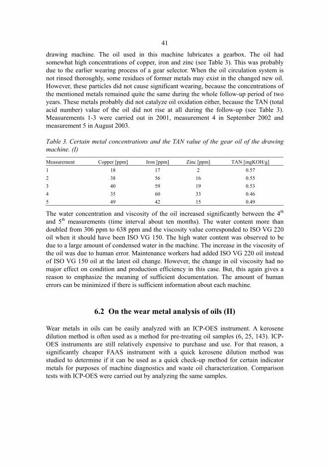
41

drawing machine. The oil used in this machine lubricates a gearbox. The oil had somewhat high concentrations of copper, iron and zinc (see Table 3). This was probably due to the earlier wearing process of a gear selector. When the oil circulation system is not rinsed thoroughly, some residues of former metals may exist in the changed new oil. However, these particles did not cause significant wearing, because the concentrations of the mentioned metals remained quite the same during the whole follow-up period of two years. These metals probably did not catalyze oil oxidation either, because the TAN (total acid number) value of the oil did not rise at all during the follow-up (see Table 3). Measurements 1-3 were carried out in 2001, measurement 4 in September 2002 and measurement 5 in August 2003.

Table 3. Certain metal concentrations and the TAN value of the gear oil of the drawing machine. (I)

Measurement Copper [ppm] Iron [ppm] Zinc [ppm] TAN [mgKOH/g] 1 18 17 2 0.57 2 38 56 16 0.55 3 40 59 19 0.53 4 35 60 33 0.46 5 49 42 15 0.49

The water concentration and viscosity of the oil increased significantly between the 4th and 5th measurements (time interval about ten months). The water content more than doubled from 306 ppm to 638 ppm and the viscosity value corresponded to ISO VG 220 oil when it should have been ISO VG 150. The high water content was observed to be due to a large amount of condensed water in the machine. The increase in the viscosity of the oil was due to human error. Maintenance workers had added ISO VG 220 oil instead of ISO VG 150 oil at the latest oil change. However, the change in oil viscosity had no major effect on condition and production efficiency in this case. But, this again gives a reason to emphasize the meaning of sufficient documentation. The amount of human errors can be minimized if there is sufficient information about each machine.

6.2 On the wear metal analysis of oils (II)

Wear metals in oils can be easily analyzed with an ICP-OES instrument. A kerosene dilution method is often used as a method for pre-treating oil samples (6, 25, 143). ICP-OES instruments are still relatively expensive to purchase and use. For that reason, a significantly cheaper FAAS instrument with a quick kerosene dilution method was studied to determine if it can be used as a quick check-up method for certain indicator metals for purposes of machine diagnostics and waste oil characterization. Comparison tests with ICP-OES were carried out by analyzing the same samples.

42

6.2.1 ICP-OES method (II)

The ICP-OES technique that was used is routinely applied in oil analysis, and similar results should be obtained in different laboratories using this technique. To clarify the functioning of the method, other sets of oil samples taken at the same time as our samples were sent to another laboratory for ICP-OES analysis. The method used there was based on the French standard NF T60-106 (145) for additive, wear metal and contaminant analysis of oils. Although sampling can affect the results, its significance was thought to be relatively minor. A paired t-test was used to compare the results of the different ICP-OES analyses. However, since the iron concentrations of the different samples varied significantly, the basic assumption of the t-test, that errors do not depend on concentration, may be violated. For this reason the t-test was divided into two categories with the results of the iron determinations: small concentrations and large concentrations. The results of the t-test are given in Table 4.

Table 4. t-test of the results of two ICP-OES analyses. (Modified thoroughly based on II and additional data)

Analyte Average difference

Deviation Degrees of freedom Calculated t-value

Critical t-value (95%)

Fe small 0.50 1.29 3 0.39 3.18 Fe large 21.50 35.42 5 1.49 2.57 Cr 3.89 9.78 8 1.19 2.31 Ni 9.29 9.41 5 2.42 2.57 Zn 0.50 2.26 5 0.54 2.57 Cu 2.25 3.01 7 2.11 2.36

The results obtained with our ICP-OES apparatus were statistically the same as the ones determined at the other laboratory. Hence, it was thought that the accuracy of our method was sufficient for the purposes of this research. Naturally, a larger amount of comparison samples would give a better picture of the properties of this method, but unfortunately that was not possible during this study.

Later, reference material (Wear Metal Multi-Element Standard, Accu Standard WM-21-NMS-30X) for wear metal analyses was purchased. However, its viscosity was very low and it was matrix-matched with Conostan 20 Base oil before it was diluted with kerosene. The results of an analysis of a 14.98 mg/l concentration of the studied metals in a kerosene solution are given as yield percentages in Table 5.

43

Table 5. Analysis of the reference material with ICP-OES. (New data)

Analyte Recovery [%] RSD [%] Fe 102.4 1.8 Cr 97.6 2.1 Ni 79.6 2.7 Zn 110.3 3.8 Cu 104.1 1.9 Recovery [%] = (Average result / 14.98 mg/l) · 100% RSD [%] = (Standard deviation / Average result) · 100%, n = 10

A big problem with this reference material was that it was not dissolved very well with Conostan S 20 Base oil and kerosene, and it tended to settle on the bottom of the ICP-OES auto sampler tubes unless shaken vigorously. However, the results of iron, chromium and copper succeeded very well indeed (results between 90-110%). The result of zinc (110.3%) is little too big and the result of nickel (79.6%) is too small. Perhaps the weak dissolution of the reference material introduced bias to these results. In addition, in some cases nickel may suffer from ionization interference. In all, the results determined with ICP-OES seemed to be accurate enough for maintenance purposes according to the reference material test, the paired t-test and various recovery tests, in which real samples were spiked with a standard material, carried out during measurements of real samples.

6.2.2 Comparison tests of ICP-OES and FAAS (II)

The results of ICP-OES were compared with FAAS by means of regression analysis at a confidence level of 95%. Both techniques employed a kerosene dilution method as a method for pre-treating oil samples. Regression analysis can reveal systematic constant errors and systematic errors depending on the concentration of the samples very effectively. The results of the regression analyses are given in Table 6.

Table 6. Regression analysis data of the comparison of ICP-OES and FAAS. (II)

Analyte Intercept (I)

Lower 95% of I

Upper 95% of I

Slope (S)

Lower 95% of S

Upper 95% of S

Adjusted R2

Obser- vations

Fe 1.368 -13.275 16.010 1.014 0.971 1.057 0.991 23 Cr 6.060 -4.190 16.309 1.033 0.966 1.099 0.978 24 Ni 1.684 -0.512 3.880 0.877 0.837 0.917 0.989 24 Zn -1.037 -2.267 0.194 0.893 0.802 0.985 0.945 24 Cu 0.065 -1.806 1.935 0.904 0.811 0.998 0.964 17

It is apparent from Table 6 that the metal concentrations determined by FAAS are relatively near to the results obtained with ICP-OES. In discussing the regression analyses of the results obtained in this study, the following observations can be made: (1) Determinations of nickel, copper and zinc using FAAS have no systematic constant error, but when compared with the results of ICP-OES, they have a small systematic error

44

that depends on concentration; (2) Determinations of iron and chromium using FAAS have no errors revealed by regression analysis when compared with the results of ICP-OES.

Nonetheless, the errors in FAAS analysis revealed by regression analysis were relatively small when compared with ICP-OES analysis. Nickel seems to have the largest error. This is probably not related to the weak recovery of the reference material when determined with ICP-OES, because the nickel determinations of the other samples succeeded well with ICP-OES. The accuracy of FAAS together with the kerosene dilution method can be sufficient enough, at least when only the magnitude of a certain metal (below or above a certain limit) is checked, i.e., in so-called semi-quantitative analysis. The observed error in the FAAS analyses that depended on concentration could possibly be diminished by using even more dilute solutions in determinations of high concentrations of metals, because the linear determination ranges of the FAAS method are narrow. When the measurements are carried out carefully, using kerosene as a solvent with FAAS does not seem to have any safety or instrumental problems with air-acetylene flame. This observation is in agreement with the study by Burrows et al. (23).

Recovery tests, in which real oil samples where spiked with varying amounts of Conostan S 21 standard, were used to reveal matrix effects in the measurements. The results of these recovery tests are presented in Table 7.

Table 7. Recovery tests determined by ICP-OES and FAAS. (II)

Analyte ICP-OES [%] FAAS [%] n Fe 104.5 ± 0.5 106.2 ± 9.3 18 Cr 98.9 ± 5.1 96.4 ± 25.7 30 Ni 97.7 ± 9.8 98.3 ± 11.9 30 Zn 96.4 ± 7.8 97.6 ± 9.9 30 Cu 95.2 ± 2.5 95.1 ± 2.5 21 n = total number of replications of different recovery tests

When determinations were carried out using ICP-OES, recoveries between 95.2% and 104.5% were obtained, depending on the studied metal. The viscosity of the oils slightly affects the recoveries. Low viscosity rolling oils are more easily nebulized into plasma than calibration standards. The recoveries of spiked metals in these oils were often between 100 and 110%. On the other hand, recovery tests in high viscosity gear oils often produced recoveries less than 100%. Variability between the times of measurement was random. In all, the recoveries were sufficient for quantitative work.

With FAAS, recovery was usually satisfactory, but standard deviations in the results were larger than with ICP-OES. For instance, with chromium the standard deviation of the recoveries was 25.7%. The reason for this might be the reduced absorption of chromium in the presence of iron and nickel and other difficulties in determination of chromium with FAAS. (151) Use of a nitrous oxide/acetylene flame could have eliminated the possible interference, (151) but introducing kerosene into a nitrous oxide/acetylene flame causes a possible safety risk. Two other possible reasons for the large standard deviations in the recovery tests with FAAS can be proposed. Particles in oil cause more atomization difficulties in a flame than in plasma due to the lower thermal

45

energy of the flame. In addition, some recovery samples had to be diluted more than the corresponding real samples in the FAAS analysis of almost all metals. Additional dilutions could increase the total uncertainty of the measurement. However, the recoveries determined with FAAS varied randomly, and FAAS with kerosene dilution is satisfactory for quantitative work with the metals studied. For instance, copper was recovered as effectively with FAAS as with ICP-OES. At least, FAAS analyses were sufficient for semi-quantitative check-ups of certain indicator metals, which are often needed by maintenance personnel.

The kerosene dilution method is a quick and effective pre-treatment method and it can be applied as well with FAAS as with ICP-OES. It can be applied with various different oils with varying metal concentrations, from low viscosity rolling oils to high viscosity gear oils.

Nevertheless, it should be noticed that metals can exist in oils in three different forms; metallic, metallic oxide or organic. The existence of certain forms depends on the metal. (34). Metallic oxides and metallo-organic species are usually very small in size (submicrons to a few microns) and easily dissolved with kerosene and detected with ICP-OES or FAAS. However, solid metal particles bigger than about 5-10 μm (the proposed critical size varies depending on the applied instrument and its properties) can not be dissolved with kerosene. Hence, the sensitivity of ICP-OES and FAAS to detect those particles decreases because plasma or a flame can not atomize them and part of them can already be lost during nebulization. The critical particle size with FAAS could be even smaller (30) than the proposed value of 5-10 μm. Nonetheless, the kerosene dilution method is widely used in wear metal analysis and wearing phenomena can usually be detected using it (see e.g., Chapters 6.1.2 and 6.1.3). Methods independent of particle size, like microwave-assisted acid digestion and ICP-OES analysis, will be developed by our research group by applying the existing standard (36) in the near future.

6.3 On the solid debris analysis of oils (III)

Solid debris analysis of oils can be used e.g., to reveal wearing mechanisms of machine elements or just to evaluate the amount of solid contaminants within lubricating oils. As seen in the literature part of this thesis (see Chapter 2.1.2) the ways of analyzing solid debris are numerous, both qualitatively and quantitatively. Experiences with the use of some methods in the analysis of stainless steel rolling oils and gear oils of a production crane are discussed in this section.

6.3.1 Membrane filtration (III)

Membrane filtration of oils is a relatively laborious and time-consuming method of studying solid matter in oils, but an estimate of oil contamination can be given by means of the solid matter concentration. Solid debris can then be studied with microscopic methods once it has been filtered out of the oil. So, membrane filtration is still an important analysis method just on its own, and especially if solid debris needs to be

46

studied more specifically. The amount of solid matter accepted in the oil circulation system depends significantly on the application area of the oil, e.g., cold rolling oils and hydraulics require very low contamination levels. The solid matter concentration data of a certain rolling oil and gear oil is presented in Table 8.

Table 8. Solid matter concentrations (> 0.45 μm) of a certain rolling oil and gear oil. (Data partially taken from III and partially new)

Measurement Rolling oil [mg/l] Gear oil [mg/l] November 2004 1 230 February 2005 < 0.5 200 June 2005 10 147.5

The rolling oil is filtered through 2 μm filter cartridges in the oil circulation system of the roller. The solid matter concentration should stay at a low level (the long-term average is under 20 mg/l) and the solid particles in rolling oil should be small, because bigger particles may cause quality defects. Black strip rolling oil is exceptional by having solid debris concentrations of over 1000 mg/l. It should be noted that black strip rolling is a different type of process than bright strip rolling, and filtration in a black strip rolling system is carried out with 50 μm band filter, thus higher solid matter concentrations are applicable. An increased solid matter concentration, like tens of mg/l, can indicate breakage of several filter cartridges in the bright strip rolling systems. As seen in Table 8, the studied gear oil has a significantly higher solid matter concentration. But these concentrations can be seen as very small when talking about gears. A solid debris level of 0.1-0.3 mass percentages i.e., even ten times as big as here, can be possible for some gears. (152)

6.3.2 Optical microscopy (III)

Optical microscopy was used to clarify the typical morphologies, quality and sizes of solid debris in certain rolling oils and gear oils of a production crane. Depending on the morphological and size properties, the particles were categorized into six different classes (rubbing, cutting, laminar, fatigue, severe sliding-type and spherical particles) according to the classification proposed by Roylance and Hunt (16).

Wear debris in rolling oils can originate from various parts of the rolling process. Possible particles may be chafed or peeled off from the product strip or worn from machine elements of the roller and then flushed into the oil circulation system. Fibreglass particles detached from oil filters may get into rolling oils during the filtration process and other non-metallic particles may be detached from coatings, valves and seals. Examples of certain categorized particles found in rolling oils are given in Figures 3 and 4.

47

Fig. 3. Cutting type particle (on the left) and laminar type particle (on the right). (New)

Fig. 4. Fatigue chunk (on the left) and severe sliding-type particle (on the right). (New and III)

The most common particles were from so-called normal wearing, i.e., rubbing particles, whose dimensions were below 20 µm. Cutting and laminar types were the most common large particles in all the oils except black strip rolling oil, where severe sliding-type particles were the most common large particles based on qualitative visual inspection. The sizes of laminars varied from 20 to even hundreds of micrometers, depending on the oil studied. Cutting-type particles could exist as long steel wires with lengths of over 1000 µm. Accurate amounts of particles could not be calculated with the microscope that was used, and therefore the evaluation of the population density of different particle categories was fully qualitative. Oxidized particles, i.e., black metal or rust, were often observed. Such particles are from the former annealing process (scale), since stainless steel does not become oxidized in the rolling process. More detailed information about the particles in rolling oils can be found in Article III.

Possible wear and contaminant particles in the gear oils of the production crane might originate from gears (steel), bearings (steel), cages (brass), axles (steel), seals (non-metals) and the environment as dust (slag, steel). The purpose was to identify and categorize the most usual solid particles in the studied gear oils in a normal situation. Examples of the particles observed in these gear oils are presented in Fig. 5.

48

Fig. 5. Laminar-type particle (on the left) and oxidized cutting type-particle (on the right). (III)

The particles of gear oils were mainly categorized as the normal wearing type, i.e., rubbing particles. On the basis of the qualitative visual inspection, the most common large particles were bright cutting and especially laminar-type metal particles. Laminar particles may be found in sizes of 30 to hundreds of micrometers and they could be bright, partially or fully oxidized. Cutting-type particles were found, e.g., in the form of long steel wires. Oxidation produced mainly black metal and sometimes rust-containing particles. If abnormal wearing of these gears occurs, the solid matter concentration should rise significantly and the morphology and quantities of the wear debris should indicate the origin and wear mechanism of those particles accurately. In a wearing situation, the amount of laminar and cutting-type particles would increase first, and in a case of severe wearing the amount of severe sliding-type particles would also begin to increase. This is in agreement with Roylance and Hunt (16), who stated that especially laminar, fatigue and severe sliding-type particles are often found in gear wear situations.

6.3.3 Scanning electron microscopy (III)

Scanning electron microscopy (SEM) can be used to determine the morphology, size and elemental distribution of solid particles captured on filter membranes. Because SEM produced elemental distribution data of solid particles, tracing their origin was possible. The solid debris of certain rolling oil samples were studied with SEM. However, SEM is not very suitable as a routine instrument, because of the moderately time-consuming pre-treatment of the membranes. In addition, only a small part of the membrane is usually cut off for SEM analysis, whereas with optical microscopy the whole membrane can be studied without destroying it. Examples of SEM images are shown in Fig. 6.

49

Fig. 6. Particles found in oils of bright strip rolling (on the left) and black strip rolling (on the right). (III)

Most of the particles within the samples were either non-reacted stainless steel from strip (Fe, Cr, Ni, Mn) or oxidized steel (Fe, Cr, Ni, Mn, O). Oxidized steel was in the form of chromium or iron oxides and was possibly scale. Oxidized steel also contained phosphorus in some cases. Phosphorus might be from the steel itself (a trace component in steel) or from an oil additive. The most typical non-metal particles were either bits of filter cartridges (e.g., C, Si, O, Cl with possible steel particles attached) or dust and slag particles (e.g., Si, O, Na, Al, K, Mg). Certain particles had a composition of Ca, O, Si and F or just Ca and F with steel. Fluorine could originate from as far as the annealing-pickling process or more likely it could be detached from the ring seals of certain bearings or hydraulic seals.

6.3.4 Automatic particle counting (III)

The total amount of particles in oils can be monitored by means of total concentrations by using membrane filtration. However, this is quite laborious, and if no qualitative/quantitative microscopic analysis is needed, then membrane filters have no extra use. The possibility of using a portable particle counter to detect particle amounts in rolling oils was checked. Determination of the amount and size distribution of solid debris in rolling oils is important in order to assure proper functioning of the filtration systems of the rollers. These tests were carried out with two different oil types from three rollers, and the oils were gathered after the machine oil filter cartridges. Particle counting data, as averages of eight or nine measurements, and membrane filtration data for the studied rolling oils are given in Table 9.

50

Table 9. Membrane filtration and particle counting data of certain rolling oils. (III)

Sample Solid matter > 0.45 µm [mg/l]

ISO Classes ≥ 4 µm / ≥ 6 µm / ≥ 14 µm

in 100 ml of oil Oil 1 in roller 1 in November 2004 9 24/21/17 Oil 1 in roller 1 in February 2005 10 24/22/13 Oil 1 in roller 2 in November 2004 5 23/21/20 Oil 1 in roller 2 in February 2005 <0.5 23/19/13 Oil 2 in November 2004 1 24/22/19 Oil 2 in February 2005 <0.5 21/16/12

Automatic particle counting produced particle quantity data accurate enough for the determination of rolling oil contamination in light of the rough comparison test made here. The low viscosity of rolling oils or the large amounts of particles, when compared with the usual application of particle counters, i.e., hydraulic oils, did not cause any observable problems. However, more tests should be carried out with other instruments in a laboratory and in the real rolling environment or even as on-line measurements. Continuous on-line measurements would probably also detect with high accuracy the very large particles (hundreds to thousands of micrometers) which are extremely harmful because of their ability to cause pebbles on the strip. But, it should be noted that it would be justifiable to use larger particle size distributions than the normal ISO classes, like particles > 50 µm and > 100 µm, in these cases. Although particle counters totally exclude particles between 0.45 µm and 4 µm, the results of the particle counter and traditional membrane filtration seemed to be somewhat comparable on a rough scale. When the total solid matter concentrations decreased, the amounts of particles detected by the particle counter decreased at least in some ISO classes (146), and vice versa. An increase in the amount of particles was also detected with both methods. Hence, automatic particle counting seems to be applicable in determining the amount of solid debris in rolling oils, at least on a rough scale. A different kind of portable particle counting system than the one used in this study has already been taken into use in monitoring the solid debris of rolling oils, and experiences with its use have been positive.

6.4 On the additive analysis of oils (IV)

Additives are vital for proper functioning of most oils. This study concentrates on analysis of fatty alcohols and fatty acid esters, which work in boundary lubrication and decrease friction in ways shown in Fig. 7.

51

+ - + -O H

CH3

+ O H

CH3

+

Metal surface

OO

Fe

O

CH3

O

CH3

Fe O O Fe

Iron oxide layerIron

Fig. 7. Physical adsorption of fatty alcohols (on the left) and chemical adsorption of fatty acid esters and fatty acids (on the right). (Modified from Kivioja et al. (153))

6.4.1 A FTIR method for analysis of fatty alcohols and fatty acid esters (IV)

The oil samples were first studied qualitatively by means of GC-MS in order to develop a FTIR method for quantitative analysis of fatty alcohols and fatty acid esters. The determined fatty alcohols and fatty acid esters in the samples are presented in Table 10.

Table 10. Fatty alcohols and fatty acid esters identified in the studied oil samples. (IV)

Fatty alcohols Fatty acid esters 1-dodecanol Hexadecanoic acid methylester = methyl palmitate 1-hexadecanol Octadecanoic acid methylester = methyl stearate 1-octadecanol 9-octadecenoic acid methylester di-2-ethylhexyladipate

Standards for quantitative FTIR analysis were chosen based on the results of the qualitative GC-MS analysis. A mixture of dodecanol, tetradecanol and octadecanol was used as hydroxyl standards in order to take into consideration the influence of the hydrocarbon chain length (82). Correspondingly, methyl palmitate and methyl stearate, which were detected in the qualitative analysis, were selected as carbonyl standards. These standards together correspond to typical fatty alcohols and fatty acid esters found in industrial oils. Toluene was used as a solvent. It has no significant spectral interference in the ranges of OH and C=O bands, and it dissolves mineral oils perfectly. It would be

52

better if no solvents were required at all, but production of a suitable concentration range for measurements and dilution of the standards was easier when a solvent was used. A suitable dilution was selected after several qualitative IR measurements.

The analytical performance of the developed FTIR method was evaluated with different tests. Recovery tests were made using two different oils, which were real samples from industry; one containing fatty alcohols and fatty acid esters (oil 1) and the other containing only fatty acid esters (oil 2). The added substances were tetradecanol and methyl stearate. The average results and their standard deviations with a confidence level of 95% obtained from different measurements during several months of the recovery tests are given in Fig. 8.

Fig. 8. Results of the recovery tests of fatty alcohol (A) and fatty acid ester (E). (IV)

The average recovery of fatty alcohol was approximately 90% with the both of the studied oils. The addition made to oil 1 was usually smaller than the corresponding addition to oil 2, because oil 1 already contained about 700 mg/kg of fatty alcohols as hydroxyl in the diluted sample. The original concentrations of fatty acid esters in the studied oils were about 500 mg/kg as carbonyl in the diluted sample. The average recovery of fatty acid ester was better in oil 1 than in oil 2; the recoveries were approximately 97% and 85%, respectively. The decreased recovery with oil 2 is probably due to the type of oil. The observed standard deviations in the determinations were mainly from measurement uncertainties that can be evaluated from the repeatability test results (see Table 11). The amount of added fatty alcohol or fatty acid ester had no significant effect on the recovery. Correction factors were not utilized, because the recoveries were sufficient for quantitative work with machinery oils.

The developed method was further tested with repeatability and reproducibility tests, whose results are given in Table 11. Three determinations were carried out in LAB 1 on three different days, and the results were tested by means of two-way ANOVA (analysis of variance). In addition, single measurements of the same samples were carried out in a different laboratory (LAB 2).

Oil 1A

n = 18

Oil 2 A

n = 11

Oil 1 E

n = 15

Oil 2 E

n = 13

0

20

40

60

80

100

120

Rec

over

y [%

]

53

Table 11. Results of the repeatability and reproducibility tests. (IV)

Sample LAB 1 OH or C=O

in oil [mg/kg]

LAB 1 SDa [mg/kg] and

(RSD)b [%]

LAB 2 OH or C=O

in oil [mg/kg]

Differencec between laboratories

[%]

FAd in oil 1 2724 39 (1.4) 2776 1.9 FA in oil 3 2688 42 (1.6) 2704 0.6 FAEe in oil 1 2094 44 (2.1) 2158 3.1 FAE in oil 2 2146 28 (1.3) 2131 -0.7 FAE in oil 3 1907 43 (2.3) 1837 -3.7 FAE in oil 4 7613 112 (1.5) 7917 4.0 FAE in oil 5 2113 48 (2.3) 2110 -0.2 a SD = standard deviation b RSD = relative standard deviation = (SD / average) · 100% c Difference [%] = [(Result of LAB 2 – Average result of LAB 1) / (Average result of LAB 1)] · 100% d Fatty alcohol e Fatty acid ester

As seen in Table 11, the relative standard deviations of the results were very small with both fatty alcohols and fatty acid esters. No statistical differences in the results within the days and between the days were observed (two-way ANOVA, p < 0.05). However, replications are worth doing in routine analyses to evaluate the daily performance of the FTIR instrument. The reproducibility test results of the fatty alcohol and fatty acid ester determinations from these samples are statistically similar, i.e., the differences between laboratories 1 and 2 were quite small.

The hydroxyl value of oils can also be determined by applying the German standard DIN 53240, but it is relatively laborious (147). A couple of determinations were carried out using this method for comparison purposes. The hydroxyl concentrations, a.k.a. the fatty alcohol concentrations, were: fatty alcohol in oil 1 ≈ 2400 mg/kg and fatty alcohol in oil 3 ≈ 2300 mg/kg. The determined concentrations were about 300 (11.9%) and 400 mg/kg (15.0%) smaller than the corresponding values determined with the IR method, respectively. This may be due to various reasons, like an improper reaction between the alcohols and acetic anhydride or problems with detection of the equivalence point or an unsuitable amount of reagents in the reaction mixture.

Carboxylic acids and water in the oil sample may introduce bias in the measurement of fatty alcohols and fatty acid esters using the FTIR method. Carboxylic acid in the sample covered the carbonyl peak of the fatty acid ester beneath its own carbonyl peak and changed the measured concentration of the carbonyl group significantly. Water moved the place of the hydroxyl peak, increased the measured concentration of the hydroxyl group and produced a shoulder next to the studied peak. The influence of the hydroxyl group of carboxylic acids on the determination of fatty alcohol was minor. The concentrations of carboxylic acids and water were known to be small in the studied real samples, hence they did not affect the results in routine measurements. In addition to chemical interferences caused by carboxylic acids and water, major sources of errors in the IR measurements are background instability, instrumental factors and scattering due

54

to large particle concentrations in used oils. Other minor sources of errors might be cross-contamination of samples, as well as adsorption and evaporation of the analytes in sample treatment.

6.4.2 Use of the developed FTIR method in routine analysis (IV)

The FTIR method developed in this work has been used successfully in both quantitative and qualitative analysis of fatty alcohols and fatty acid esters. The concentrations of these additives were monitored in the oils of certain production machines over a period of 10 months. The results are given in Fig. 9 where measurements 1-4 were carried out in April 2004, August 2004, November 2004 and February 2005, respectively.

Fig. 9. Quantitative analysis of fatty alcohols and fatty acid esters. (IV)

In another case, we wanted to know if drawing oil entered into the gear oil and if a change of the drawing oil and gear oil was required. Contamination of the gear oil with the drawing oil is a direct indication of breakage of seals in the machine. The gear oil and all the seals of the machine have to be replaced if the contamination occurs. These repairs require work by two maintenance workers for one week in addition to production losses. Hence, replacement of the seals has to happen based on condition and not unnecessarily. The developed FTIR method was applied to this study. Samples of new drawing oil, new gear oil, used drawing oil and used gear oil were analyzed with the FTIR method. The resulting spectra are shown in Fig. 10.

1500170019002100230025002700290031003300

1 2 3 4

Measurement

OH

or

C=O

[mg/

kg]

Oil 1 FattyalcoholOil 1 Fattyacid esterOil 2 Fattyacid ester

55

Fig. 10. Spectra of drawing and gear oil samples. (New)

A very intense peak caused by an ester carbonyl group was observed at 1743 cm-1 as well as several peaks at 1300-1100 cm-1 in the spectrum of the new drawing oil. Similar peaks were observed in the spectrum of the used drawing oil, but significantly weaker. The lower intensity of these peaks might be due to consumption of corresponding additives. The significant increment of the background level in the spectrum of the used drawing oil was due to scattering caused by a large amount of solid particles in this sample. So, the drawing oil needed to be changed.

As seen from the spectrum of the new gear oil, it has neither peaks at the carbonyl area nor at 1300-1100 cm-1. So, the gear oil and the drawing oil can be separated with the help of these peaks. When looked at the spectrum of the used gear oil, no peaks at 1743 cm-1 or 1300-1100 cm-1 are observed. This means there was no drawing oil in the gear oil and neither the gear oil nor the seals had to be changed. It should be noted that when the gear oil was mixed with the drawing oil on purpose (10% drawing oil/90% gear oil), the carbonyl peak and the peaks at 1300-1100 cm-1 were observed clearly. So, the contamination of the gear oil with the drawing oil can be observed at least when it has greater significance to the functioning of the gear oil and the machine.

6.5 Biodegradability studies of oils (V, VI)

The environmental effects of selected oils were evaluated by means of biodegradability studies. The biodegradation of certain forestry hydraulic oils (Article V) was studied in different waters, e.g., in groundwater and in conditions described by OECD 301 F (114). In addition, the biodegradation of certain forestry chain oils and wood preservative oils (Article VI) was studied in forest soils. The biodegradation of these oils has also been studied in a water medium in other articles (154-155). All the measurements were carried out with the automatic, respirometric BOD OxiTop method.

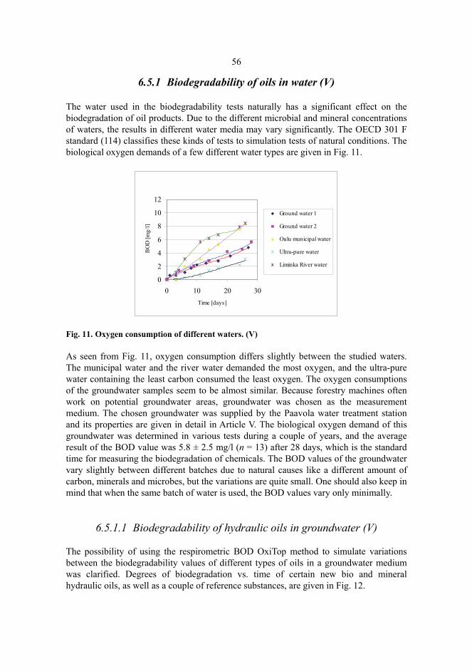
56

6.5.1 Biodegradability of oils in water (V)

The water used in the biodegradability tests naturally has a significant effect on the biodegradation of oil products. Due to the different microbial and mineral concentrations of waters, the results in different water media may vary significantly. The OECD 301 F standard (114) classifies these kinds of tests to simulation tests of natural conditions. The biological oxygen demands of a few different water types are given in Fig. 11.

Fig. 11. Oxygen consumption of different waters. (V)

As seen from Fig. 11, oxygen consumption differs slightly between the studied waters. The municipal water and the river water demanded the most oxygen, and the ultra-pure water containing the least carbon consumed the least oxygen. The oxygen consumptions of the groundwater samples seem to be almost similar. Because forestry machines often work on potential groundwater areas, groundwater was chosen as the measurement medium. The chosen groundwater was supplied by the Paavola water treatment station and its properties are given in detail in Article V. The biological oxygen demand of this groundwater was determined in various tests during a couple of years, and the average result of the BOD value was 5.8 ± 2.5 mg/l (n = 13) after 28 days, which is the standard time for measuring the biodegradation of chemicals. The BOD values of the groundwater vary slightly between different batches due to natural causes like a different amount of carbon, minerals and microbes, but the variations are quite small. One should also keep in mind that when the same batch of water is used, the BOD values vary only minimally.

6.5.1.1 Biodegradability of hydraulic oils in groundwater (V)

The possibility of using the respirometric BOD OxiTop method to simulate variations between the biodegradability values of different types of oils in a groundwater medium was clarified. Degrees of biodegradation vs. time of certain new bio and mineral hydraulic oils, as well as a couple of reference substances, are given in Fig. 12.

0

2

4

6

8

10

12

0 10 20 30Time [days]

BO

D [m

g/l]

Ground water 1

Ground water 2

Oulu municipal water

Ultra-pure water

Liminka River water

57

Fig. 12. Plots of BOD/ThOD vs. time for certain new hydraulic oils and reference substances in groundwater. (V)

Sodium acetate and sodium benzoate, which should be quickly biodegrading substances, were used as reference substances. They should reach a BOD/ThOD value of 60% in 10 days in suitable conditions (114). The degree of biodegradation of sodium acetate after 28 days was only 7.3% in the groundwater used. A replication test gave a slightly smaller BOD/ThOD value of 5% after 28 days. The degree of biodegradation of sodium benzoate in groundwater was only slightly higher (10.1% after 28 days) than the corresponding value of sodium acetate. However, some of the oils seemed to biodegrade easier than sodium acetate and sodium benzoate in groundwater conditions. Sodium acetate and sodium benzoate could be difficult to biodegrade without minerals, or the groundwater used does not contain suitable microbes for their degradation. When biodegradation tests of these reference substances were carried out in the standard conditions described by OECD 301 F (114), the results were completely different.

Sodium acetate reached the BOD/ThOD value of over 80% already after five days in the standard conditions and sodium benzoate biodegraded at a similar rate as sodium acetate. So, the reason for the low degrees of biodegradation of these substances in groundwater was the lack of suitable microbes and minerals. More likely the reason was the lack of minerals in groundwater, because the degree of biodegradation of sodium acetate in groundwater, to which minerals were added in suitable concentrations, was over 60% after five days. Hence, the microbes in the groundwater used seemed to be efficient in biodegrading sodium acetate if enough minerals were present.

As seen from Fig. 12, mineral oils biodegraded slowly in groundwater, but bio oils 3 and 4 did not exactly biodegrade any better. Bio oils 1 and 2 seemed to biodegrade significantly better. The degree of biodegradation of bio oils 1 and 2 after 28 days in groundwater was over 20%, which could be an indication of a potentially degrading substance in groundwater. A direct comparison of these results with the results of tests done under optimal conditions is difficult, because the reference substances behave so differently in groundwater than in the mineral and microbe-containing medium.

One purpose of this study was to clarify how the use of oils affects the degree of biodegradation of oils, if at all. Information on the behaviour of used oils in groundwater is important, because a majority of oil spillages occur during use of oil, and the

05

101520253035

0 5 10 15 20 25 30

Time [days]

BO

D/T

hOD

[%]

Bio oil 1Bio oil 2Bio oil 3Bio oil 4Mineral oil 1Mineral oil 2Sodium acetateSodium benzoate

58

biodegradability data of new oils can not necessarily be applied. Biodegradability tests of certain new and used hydraulic oils in a groundwater medium are presented in Fig. 13.

Fig. 13. Plots of BOD/ThOD vs. time for new and corresponding used (taken from oil changes) hydraulic oils in groundwater. (V)

As seen from Fig. 13, all the used hydraulic oils studied here biodegraded in a lesser degree than the corresponding new ones, and the change in the biodegradation rate after use of the bio oils seemed to be significant. With the mineral oils the corresponding change was smaller. Used bio oil 3 even seemed to biodegrade as slow as mineral oil 1 in groundwater. Based on this study, used bio oil 3 can not be claimed to be easily biodegradable in a groundwater environment, when even mineral oil biodegrades at an equal rate. The reason for the slower biodegradation of used oils might be degradation of certain components of the oil during use or evaporation of volatile substances. Certain metals (like zinc and nickel) within oils can catalyze the degradation of oil during use (156). These kinds of catalyzed reactions were not probable with these oils because their metal concentrations were very small.

The precision of the BOD OxiTop method in determining the biodegradability of oils was studied using the following test. The BOD values of three different samples of the same bio oil (bio oil 5) were determined using the BOD OxiTop method. The average BOD/ThOD value calculated for this oil was 32.08 ± 0.34% after 32 days, RSD was 1.06%. The precision of the BOD OxiTop method was also tested with chain oils in another study (154). The RSD values of replication tests carried out in that study varied between 0.48 and 4.72% (154). So, the precision of the BOD OxiTop method was good enough for analytical determinations of the BOD values of oils. What is still important to notice is that bio oil 5 biodegraded quite effectively (BOD/ThOD > 30% after 28 days) in a groundwater environment.

6.5.1.2 Biodegradability of hydraulic oils in standard conditions (V)

The biodegradation of new bio hydraulic oils studied in a groundwater environment was also examined in standard conditions described by the OECD 301 F standard (114). The

0

5

10

15

20

25

30

35

0 5 10 15 20 25 30

Time [days]

BO

D/T

hOD

[%]

Bio oil 1 newBio oil 1 usedBio oil 3 newBio oil 3 usedMineral oil 1 newMineral oil 1 usedMineral oil 2 newMineral oil 2 used

59

degrees of biodegradation of these bio oils in the conditions described by OECD are shown in Fig. 14.

Fig. 14. Biodegradability tests of new bio hydraulic oils in an extra mineral and microbe-containing medium described by OECD 301 F. (V)

Bio oil 5 biodegraded fastest and bio oil 1 slowest; the degrees of biodegradation after 28 days were 89.1% and 25.6% respectively. The behaviour of bio oil 5 was as expected, because the value of its degree of biodegradation was definitely the biggest (> 30%) also in the groundwater environment. The behaviour of bio oil 1 was surprising, because when compared with the results in the groundwater environment, the degrees of biodegradation were almost the same after 28 days. No simple explanation for this observation can be given. The microbes of both environments seem to be efficient enough to biodegrade certain components of bio oil 1. Bio oils 2-4 were all moderately well biodegradable (BOD/ThOD values varied between 36.9 and 49.0% after 28 days) in the biodegradability tests in an additional mineral and microbe-containing medium, and the change of conditions from groundwater to more optimal seemed to double or even triple the degrees of biodegradation.

OECD 301 F (114) also requires an estimation of abiotic degradation, which can be significant with quickly biodegrading substances. Bio oils 1-5 were also degraded in abiotic conditions. The abiotic degradation was rather minor with these oils, the degradation percentages being between 1.4 and 2.6%, depending on the oil studied.

6.5.2 Biodegradability of oils in soil (VI)

The biodegradation of different chain oils and wood preservative oils was studied in different soils. The exact properties of these soils (marked as soil 1, 2, 3s and 3d) are given in detail in Article VI. All the soils were sampled in August 2003. Soils 3s and 3d were sampled from the same place; 3s from the surface and 3d from deeper. Soil 3s was most fertile, because the forest area had been fertilized with NPK fertilizer earlier. Soil 3s also had the biggest content of organic matter. The same soil, when sampled from a deeper layer (3d), had significantly lower amounts of basic nutrients and organic matter. All the soils except soil 1 were categorized as coarse mineral soils. All the soils were

0102030405060708090

100

0 5 10 15 20 25 30

Time [days]

BO

D/T

hOD

[%] Bio oil 1

Bio oil 2Bio oil 3Bio oil 4Bio oil 5

60

moderately acidic, but the observed acidities were excellent for forest soils. The conductivity of certain soils (1 and 3s) was rather high.

We wanted to evaluate the suitability of the BOD OxiTop method in determining the biodegradation of oils in soil, hence the biodegradation of a typical oil sample was determined in the collected soil samples. Tall oil fatty acid (TOFA) was chosen to be the model oil in this particular case. It was formerly observed to be moderately biodegradable in groundwater and in the standard conditions described by OECD 301 F (155). Biodegradation of TOFA in different soils is presented in Fig. 15.

Fig. 15. BOD/ThOD value vs. time for tall oil fatty acid (TOFA) in different soils. (VI)

TOFA biodegraded most effectively in soil 3s; the degree of biodegradation was over 45% after 14 days. The obvious reason for this observation is that soil 3s had neither microbial nor nutrient limitations. Based on the results obtained in this test, soil 3s was used in all other biodegradation tests in order to facilitate the quickest possible biodegradation reactions of oils within these soils. Soil 2 and 3d would also have been moderately good media for measuring the biodegradation of oils; the BOD/ThOD values of TOFA varied between 34.9% and 37.5% after 14 days. But the biodegradation of TOFA in soil 1 was quite poor, possibly due to nutrient limitation. Replicate tests of the biodegradation of TOFA in different soils revealed that the precision of the BOD OxiTop method in these measurements was rather good.

The suitability of the selected soil 3s for oil biodegradation measurements was also tested with sodium acetate and sodium benzoate known to be quickly biodegrading in suitable conditions. A limit value for ready biodegradability is 60% in 10 days, and both sodium acetate and sodium benzoate reached this limit, and after 14 days their BOD/ThOD values were 89.9% and 85%, respectively. Hence, the selected soil 3s was suitable for biodegradability evaluation tests.

The biodegradation of certain wood preservative oils and chain oils was evaluated with the BOD OxiTop method in the selected soil 3s. When discussing about wood preservatives, the following observations could be made. Linseed oil reached a moderate BOD/ThOD value of 42.9% after 14 days, but the experimental substances, which were derivatives of tall oil fatty acid (TOFA), reached even higher values. Creosote oil also

0

5

10

15

20

25

30

35

40

45

50

0 5 10 15

Time [days]

BO

D/T

hOD

[%]

Soil 1

Soil 1

Soil 2

Soil 3s

Soil 3s

Soil 3d

Soil 3d

61

biodegraded moderately in this soil, but it reached a stable phase with a BOD/ThOD value of 25% during the measurement, and most likely it will not biodegrade significantly better in longer-lasting measurements. On the other hand, biodegradation of the other wood preservatives was still effective after 14 days, and a longer incubation time would have produced even higher BOD/ThOD values.

The studied forestry chain oils were rapeseed oils and tall oil. Rapeseed oils biodegraded better than tall oil in these experiments. Similar observations have been formerly made in a water medium (154). The degrees of biodegradation of rapeseed oils after 14 days varied between 33.3% and 44.5% in soil 3s, while tall oil had a BOD/ThOD value of 27.8% during the same time. However, a longer incubation period will produce higher values of BOD/ThOD, because none of these oils reached a stable phase of biodegradation in 14 days. Replicates of rapeseed oil 1 gave quite similar results (the BOD/ThOD values were 41.4% and 44.5% after 14 days) in soil 3s, hence the precision of the method was rather good in measurements in a soil medium. Of course, replication tests give more precise results in water, which is a more homogenous measurement medium (154).

7 Conclusions

This study gathers together various condition monitoring methods, however, it mainly concentrates on oil analysis methods. The life cycle of oil products consists of raw oil utilization, refining and other production processes, transportation and storage of the oil products, their useful life and oil waste management. This study focuses on the use of oil products and expanding their useful life by gathering information on the condition of lubrication oils with oil analysis methods. On the other hand, oil can reveal information about the condition of machine elements which it lubricates, just like a blood test can tell about the “condition of a human”. In addition, the environmental effects of certain oil products were evaluated with biodegradation measurements. The main emphasis of this study was on developing and tuning oil analysis methods to meet the condition monitoring requirements of modern industry and the demands of environmental analytics.

As a special case, the condition of worm gears in different fields of industry was monitored. Worm gears are relatively difficult to monitor with traditional vibration monitoring because the contact between the worm and the worm wheel is sliding, and not necessarily periodical impact-like phenomena occur in failure situations as is usual with other gears. Vibration analysis of worm gears is possible, but detection of wearing demands thorough analysis of especially the higher frequency area and also the time domain signal. Normal features, like kurtosis and crest factor, were not useful. The most sensitive feature in monitoring the studied worm gears seemed to be the rms value of x(3) in the frequency range 10-2000 Hz. Analysis of wear metals in gear oils was usually a significantly easier way to analyze wearing of worm gears and measurement of copper and iron was enough, because they are main components in worm wheels and worms, respectively. A good way is to unite both methods, where wear metal analysis detects wearing processes and vibration monitoring detects e.g., unbalance and electrical problems of motors.

Effective wear metal analysis requires suitable analysis methods. ICP-OES employing the kerosene dilution method is widely used in wear metal analyses. ICP-OES is expensive to purchase and use, hence the cheaper FAAS method was tested together with the rapid kerosene dilution method as a pre-treatment of oil samples. One should keep in mind that the kerosene dilution method always has problems with solid particles bigger than 10 μm, because kerosene does not dissolve them and their nebulization efficiency to

63

plasma or a flame as well as their atomization sensitivity decreases. When comparing the ICP-OES with FAAS with both employing kerosene dilution, the observations were that determinations of nickel, copper and zinc using FAAS have no systematic constant error, but they have a small systematic error that depends on concentration, and determinations of iron and chromium with FAAS have no errors revealed by regression analysis. Recoveries obtained with the FAAS method were also usually satisfactory for analyzing wear metals of oils, but the standard deviations of the recoveries were larger than with ICP-OES. The largest standard deviations were observed with chromium, but for example copper was recovered with FAAS as effectively as with ICP-OES. In all, FAAS with the kerosene dilution showed sufficient accuracy for wear metal analysis in machine diagnostics and waste oil characterization, at least in a semi-quantitative manner. Especially if only a couple of indicator metals from a few samples are measured, FAAS is highly suitable.

Solid debris analysis of certain rolling and gear oils was carried out using different methods. Membrane filtration can be used to evaluate the solid matter concentrations of oils and membrane filters can be studied with different microscopic methods. Solid particles of rolling and gear oils were categorized into different classes by optical microscopy in order to clarify their origin and wearing mechanism. Cutting and laminar-type particles were the most common large particles in all rolling oils, except in black strip rolling oil, where severe sliding-type particles were the most common large particles. Cutting-type and especially laminar-type particles were typical large particles in gear oils of the production crane. Optical microscopy is a useful method for analyzing the morphology, quality and size of solid particles qualitatively, and it does not require any pre-treatment of the studied membranes. Scanning electron microscopy (SEM) was suitable for determining the elemental distribution of particles, but it requires pre-treatment of the samples. The most usual particles in rolling oils were stainless steel-based as such or in oxidized forms (scale). Sometimes also parts of filter cartridges and seals could be observed, as well as dust. Because the membrane filtration method is relatively laborious, other methods for determining particle concentrations of rolling oils were sought. Automatic particle counting seemed to be suitable for determining particle quantities in rolling oils, and it has already been taken into use in the rolling plant. But, it must be emphasized that the normal ISO classes may not be enough, it is often more useful to determine larger-size classes e.g., > 50 μm and > 100 μm. This is also important with rolling oils, and suitable particle counters are commercially available.

The ability to analyze oil additives is vital in many cases because additives make proper functioning of the oil possible. A quantitative FTIR analysis method for analyzing concentrations of fatty alcohols and fatty acid esters in machinery oils was developed in this study. The developed method does not require highly volatile and toxic solvents, like CCl4, and it proved to be accurate and precise for quantitative work. The applicability of this method was tested with real oil samples and recovery samples. Its repeatability and reproducibility was also clarified and some comparison measurements of fatty alcohols were carried out with a standardized method. Possible errors of the developed method were also evaluated in a qualitative manner. The method has already been used successfully in quantitative and qualitative analysis of various oil samples.

Biodegradation measurements were used to evaluate the environmental effects of certain oils in water and soil media. An automatic, respirometric BOD OxiTop method

64

was used in all the measurements. Wood harvesters and forwarders often work in groundwater areas, hence the biodegradation of certain mineral and bio hydraulic oils was studied in a groundwater environment. The type of oil influences its biodegradability. Mineral oils usually biodegraded in a lesser degree than bio oils in groundwater. The use of oils had a significant effect on the biodegradation ability of hydraulic oils, especially with bio oils. Used bio oils biodegrade significantly slower than corresponding new ones. All bio oils except bio oil 1 biodegraded significantly faster in the standard conditions described by OECD 301 F than in groundwater. Especially the extra minerals seemed to be important, because the microbes of groundwater could adapt to biodegrade oils. Abiotic degradation of hydraulic oils was rather minor. The suitability of the BOD OxiTop method for biodegradation measurements of chemicals was tested with sodium acetate and sodium benzoate, which are known to be quickly biodegrading substances in suitable conditions. The precision of the method in measurements of oil biodegradation in a water medium was also determined, and it was shown to be good.

Forestry chain oils and oils used to preserve wood-based structures may be in contact with soils. Hence, their biodegradation was studied in different forest soils. The soil suitable for effective biodegradation of oils was searched for using tall oil fatty acid (TOFA) as a model substance. Soil 3s seemed to be the most suitable and it was tested as a measurement medium with sodium acetate and sodium benzoate. The precision of the BOD OxiTop method also seemed to be rather good in soil measurements. Experimental wood preservatives biodegraded quite effectively in the selected soil 3s. Linseed oil, which is used as a natural wood preservative, also biodegraded moderately in soil 3s. On the other hand, the widely used wood preservative creosote oil biodegraded in a lesser degree and reached a stable phase during the 14 days of measurement. Rapeseed chain oils biodegraded more effectively than corresponding tall oil.

However, it should be noted that we had no possibility to measure the oxygen concentration of the oils and calculations of theoretical oxygen demand were carried out using only carbon concentrations. Hence, the measured BOD/ThOD values may be too big in some cases when calculated using only the main component of oils, i.e., carbon, but at least the results are fully comparable with each other.

8 Future work

There is wide interest in the maintenance departments of our industrial partners in monitoring the condition of worm gears, because there are no simple methods available for this purpose. The aim is to use different monitoring methods, like oil analysis and vibration analysis, to find out the best features for measuring the condition of worm gears in industrial applications. This study has already started. A laboratory test rig containing a worm gear will also be constructed in the long run.

A microwave-assisted acid digestion method will be developed applying the standard US EPA 3051A for pre-treatment of oil samples before wear metal analysis. When the oils are totally degraded, also the large solid debris particles are detected with ICP-OES or FAAS very sensitively. The plan is first to optimize the digestion method and then the ICP-OES measurement. This work has already begun and results will be published in the near future. The best possible combination of methods for monitoring solid debris qualities and quantities in different oils will be sought. FTIR methods for determining other types of additives than in this study would be interesting to develop in the future.

Biodegradation studies of different kinds of chemicals using the BOD OxiTop method will be continued in the research group both in different waters and in soils. This is an important issue because according to environmental laws, the biodegradation potential of all new chemicals has to be evaluated. The study of oil-contaminated soils is already ongoing. Hopefully, there will also be a possibility to purchase an elemental analyzer which is capable of determining oxygen, hence making calculations of the degrees of biodegradation more accurate.

References

1. Öljy- ja Kaasualan Keskusliitto. Tilastot, http://www.oil-gas.fi. Site visited in 20.04.06. 2. Ahlroos T (2003) Tribologia, voitelu ja ympäristöasiat. Tribologia – Finnish Journal of

Tribology 22 No 4 23–29. 3. Teollisuusvoitelu (2003) KP-Media Oy, Rajamäki, Finland. 4. Järviö J (ed.) (2004) Kunnossapito. KP-Media Oy, Rajamäki, Finland. 5. Rao BKN (ed.) (1996) Handbook of Condition Monitoring. Elsevier Science Ltd, Oxford,

UK. 6. Toms LA (1998) Machinery Oil Analysis – Methods, Automation & Benefits. Coastal

Skills Training, Virginia Beach, USA. 7. Nordic Guidelines on Life-Cycle Assessment (1995) Nordic Council of Ministers,

Copenhagen, Denmark. 8. Hägg B (2005) The great profitability potential in manufacturing industry. In: Lahdelma

S & Palokangas K (eds) Proc of the 2nd Int Seminar of Maintenance, Condition Monitoring and Diagnostics, Oulu, Finland, 28th – 29th September 2005, 7–16.

9. Hunt T & Evans J (2004) Oil analysis handbook. Coxmoor publishing company, Oxford, UK.

10. Crawford AR & Crawford S (1992) The simplified handbook of vibration analysis. Vol 1: Introduction to Vibration Analysis Fundamentals & Vol 2: Applied Vibration Analysis. Computational Systems, Knoxville, USA.

11. Klein U (2000) Schwingungsdiagnostische Beurteilung von Maschinen und Anlagen. Stahl Eisen, Düsseldorf, Germany.

12. Barthel K (1977) The shock pulse method for measuring the condition of antifriction bearings. Tappi 60 No 8 111–113.

13. Spanner JC (1974) Acoustic Emission – Techniques and Applications. Intex Publishing Company, Evanston, USA.

14. Mba D & Rao RBKN (2005) Development of Acoustic Emission Technology for Condition Monitoring and Diagnosis of Rotating Machines; Bearings, Pumps, Gearboxes, Engines and Rotating Structures. The Shock and Vibration Digest 37 No 5 1–57.

15. Bøving KG (ed.) (1989) NDE handbook: non-destructive examination methods for condition monitoring. Butterworths, London, UK.

16. Roylance BJ & Hunt TM (1999) The Wear Debris Analysis Handbook. Coxmoor publishing company, Oxford, UK.

17. Niiranen E (2004) Hiukkaslaskenta öljyjärjestelmien kunnonvalvonnassa. Tribologia – Finnish Journal of Tribology 23 No 3–4 5–15.

67

18. Raadnui S & Kleesuwan S (2005) Low-cost condition monitoring sensor for used oil analysis. Wear 259:1502–1506.

19. Parikka R & Vaajoensuu E (2003) Valon läpäisyyn perustuvat low cost-analysaattorit öljyjen käynninaikaiseen kunnonvalvontaan. Tribologia – Finnish Journal of Tribology 22 No 4 16–22.

20. Raadnui S (2003) Transmission condition evaluation through magnetic chip detector (MCD) ferrous wear particle analysis. In: Shrivastav OP, Al-Najjar B & Rao RBKN (eds) Proc of the 16th Int Congress of COMADEM, Växjö, Sweden, 27th – 29th August 2003, 473–479.

21. Skoog DA & Leary JJ (1992) Principles of Instrumental Analysis. Harcourt Brace & Company, Orlando, USA.

22. Kellner R, Mermet J-M, Otto M & Widmer HM (eds) (1998) Analytical Chemistry – The Approved Text to the FECS Curriculum Analytical Chemistry. Wiley-VCH Verlag GmbH, Weinheim, Germany.

23. Burrows JA, Heerdt JC & Willis JB (1965) Determination of Wear Metals in Used Lubricating Oils by Atomic Absorption Spectrometry. Anal Chem 37:579–582.

24. Lukasiewicz RJ & Buell BE (1975) Study of Zinc Determination in Lubricating Oils and Additives by Atomic Absorption Spectrometry. Anal Chem 47:1673–1676.

25. de la Guardia M & Salvador A (1984) Flame atomic absorption determination of metals in lubricating oils: a critical review. At Spectrosc 5:150–154.

26. King AD, Hilligoss DR & Wallace GF (1984) Comparison of results for determination of wear metals in used lubricating oils by flame atomic absorption spectrometry and inductively coupled plasma emission spectrometry. At Spectrosc 5:189–191.

27. Berndt H, Schaldach G & Kägler SH (1996) Flame AAS/flame AES for trace determination in fresh and used lubricating oils with sample introduction by hydraulic high-pressure nebulization. Fresenius J Anal Chem 355:37–42.

28. Mora J, Todolí JL, Sempere FJ, Canals A & Hernandis V (2000) Determination of metals in lubricating oils by flame atomic absorption spectrometry using a single-bore high-pressure pneumatic nebulizer. Analyst 125:2344–2349.

29. Jansen EBM, Knipscheer JH & Nagtegaal M (1992) Rapid and Accurate Element Determination in Lubricating Oils Using Inductively Coupled Plasma Optical Emission Spectrometry. J Anal At Spectrom 7:127–130.

30. Jantzen E, Buck V & Kaegler SH (1983) Influence of particle size on wear assessment by spectrometric oil analysis. I: Atomic absorption spectrometry. Wear 87:331–338.

31. Guinat E (1985) Spectrometric oil analysis: Atomic emission spectrometric analysis of wear metals in lube oils by RDE method. Tribology International 18:246.

32. Kauffmann RE (1989) Particle Size and Composition Analyses of Wear Debris Using Atomic Emission Spectrometry. Lubrication Engineering 45:147–153.

33. Klaentschi N (1984) ICP emission spectrometry: Effect of the particle size in the determination of wear elements in lubricating oils. Material & Technik 12:3–7.

34. Kauffmann RE, Saba CS, Rhine WE & Eisentraut KJ (1985) Chemical Nature of Wear Debris. ASLE Transactions 28:400–406.

35. Lunde L, Thoresen H & Wahlstrøm E (2001) Condition monitoring of thruster systems using oil analysis. Tribologia – Finnish Journal of Tribology 20 No 1 31–40.

36. USEPA (1998) Method 3051A: Microwave assisted acid digestion of sediments, sludges, soils and oils, Revision 1.

37. Sanz-Segundo C, Hernández-Artiga MP, Hidalgo-Hidalgo de Cisneros JL, Bellido-Milla D & Naranjo-Rodriguez I (1999) Determination of Wear Metals in Marine Lubricating Oils by Microwave Digestion and Atomic Absorption Spectrometry. Mikrochim Acta 132:89–94.

68

38. Wang T, Jia X & Wu J (2003) Direct determination of metals in organics by inductively coupled plasma atomic emission spectrometry in aqueous matrices. J Pharm Biomed Anal 33:639–646.

39. Udoh AP (1995) Determination of calcium, magnesium and zinc in unused lubricating oils by atomic absorption spectroscopy. Talanta 42:1827–1831.

40. Barbooti MM, Zaki NS, Baha-Uddin SS & Hassan EB (1990) Use of silica-gel in the preparation of used lubricating oil samples for the determination of wear metals by flame atomic absorption spectrometry. Analyst 115:1059–1061.

41. Souza RM, da Silveira CLP & Aucélio RQ (2004) Determination of Refractory Elements in Used Lubricating Oil by ICPOES Employing Emulsified Sample Introduction and Calibration with Inorganic Standards. Anal Sci 20:351–355.

42. Thiem TL & Watson JD (1997) Extraction Efficiencies of Emulsions for 21 Elements in Oil and Transmission Fluids by Inductively Coupled Plasma Spectroscopy. Microchem J 57:245–250.

43. Murillo M, Gonzalez A, Ramirez A & Guillen N (1994) Determination of Metals in Lubricating Oils by ICP-OES With Emulsion Sample Introduction. At Spectrosc 15:90–95.

44. Lakatos J, Lakatos I & Bagdi G (1996) Application of Emulsions for Direct Flame Atomic Absorption Spectrometric Analysis of Organic Liquids. Microchem J 54:303–319.

45. Goncalves IM, Murillo M & González AM (1998) Determination of metals in used lubricating oils by AAS using emulsified samples. Talanta 47:1033–1042.

46. Kauffmann RE, Saba CS, Rhine WE & Eisentraut KJ (1982) Quantitative Multielement Determination of Metallic Wear Species in Lubricating Oils and Hydraulic Fluids. Anal Chem 54:975–979.

47. Escobar MP, Smith BW & Winefordner JD (1996) Determination of metallo-organic species in lubricating oil by electrothermal vaporization inductively coupled plasma mass spectrometry. Anal Chim Acta 320:11–17.

48. Bings NH (2002) Direct determination of metals in lubricating oils by laser ablation coupled to inductively coupled plasma time-of-flight mass spectrometry. J Anal At Spectrom 17:759–767.

49. Liu Y-W, Harding AR & Leyden DE (1986) Determination of wear metals in oil using energy dispersive X-ray spectrometry. Anal Chim Acta 180:349–355.

50. Pouzar M, Černohorský T & Krejčová A (2001) Determination of metals in lubricating oils by X-ray fluorescence spectrometry. Talanta 54:829–835.

51. Yang Z, Hou X & Jones BT (2003) Determination of wear metals in engine oil by mild acid digestion and energy dispersive X-ray fluorescence spectrometry using solid phase extraction disks. Talanta 59:673–680.

52. Fischer GC & Hiltz JA (2001) Identification of non-metallic particulate in lubricant filter debris. In: Starr AG & Rao RBKN (eds) Proc of the 14th Int Congress of COMADEM, Manchester, UK, 4th – 6th September 2001, 959–966.

53. Chander T & Biswas S (1983) Abnormal wear of gear couplings – a case study. Tribology International 16:141–146.

54. Chiou Y-C, Lee R-T & Tsai C-Y (1998) An on-line Hall-effect device for monitoring wear particle in oils. Wear 223:44–49.

55. Saba CS (1989) Determination of metallic iron in wear debris using a wear particle analyzer. Wear 129:143–158.

56. Myshkin NK, Markova LV, Semenyuk MS, Kong H, Han H-G & Yoon E-S (2003) Wear monitoring based on the analysis of lubricant contamination by optical ferroanalyzer. Wear 255:1270–1275.

69

57. Roylance BJ (2005) Ferrography – then and now. Tribology International 38:857–862. 58. PAMAS. Products, http://www.pamas.de. Site visited in 20.04.06. 59. HYDAC International. Products, http://www.hydac.com. Site visited in 20.04.06. 60. Day MJ & Rinkinen J (1997) Contaminant monitoring of hydraulic systems – the need

for reliable data. In: Jantunen E, Holmberg K & Rao RBKN (eds) Proc of the 10th Int Congress of COMADEM, Espoo, Finland, 9th – 11th June 1997, Vol 1, 171–182.

61. Day MJ (1999) “Condition Monitoring of Fluid Systems – The Need for A Systematic Approach”. In: Jones MH & Sleeman DG (eds) Proc of the Int Conference on Condition Monitoring, Swansea, UK, 12th – 15th April 1999, 487–505.

62. Tucker JE, Schultz A, Lu C, Sebok T, Holloway C, Tankersley LL, McClelland T, Howard PL & Reintjes J (1999) LASERNET FINES Optical Wear Debris Monitor. In: Jones MH & Sleeman DG (eds) Proc of the Int Conference on Condition Monitoring. Swansea, UK, 12th – 15th April 1999, 445–452.

63. Heikkinen K (2003) Öljyn puhtauden valvonta. In: Malcast Oy (org.) Fluid Forum 2003 – Teema: Hydrauliikka. Tampere, Finland, 19th – 20th March 2003.

64. Vesala M (2005) Pieniä hiukkasia, joilla on suuri merkitys. Fluid Finland 4 No 1 22–27. 65. Myshkin NK, Kong H, Grigoriev AY & Yoon E-S (2001) The use of color in wear debris

analysis. Wear 251:1218–1226. 66. Akagaki T & Kato K (1991) Effects of additives on wear mode and morphology of wear

debris generated in the lubricated sliding of steel. Wear 143:119–135. 67. Wang L, Wood RJK, Harvey TJ, Morris S, Powrie HEG & Care I (2003) Wear

performance of oil lubricated silicon nitride sliding against various bearing steels. Wear 255:657–668.

68. Scherge M, Martin JM & Pöhlmann K (2006) Characterization of wear debris of systems operated under low-wear rate conditions. Wear 260:458–461.

69. Peng Z & Kirk TB (1998) Automatic wear-particle classification using neural networks. Tribology Letters 5:249–257.

70. Peng Z & Goodwin S (2001) Wear-debris analysis in expert systems. Tribology Letters 11:177–184.

71. Peng Z (2002) An integrated intelligence system for wear debris analysis. Wear 252:730–743.

72. Wills JG (1980) Lubrication fundamentals. Marcel Dekker Inc, New York, USA. 73. Braithwaite ER (ed.) (1967) Lubrication and lubricants. Elsevier Publishing Company,

Essex, UK. 74. Adgar A, Schwarz MH & MacIntyre J (2004) Development of intelligent software for a

micro-sensor based oil quality analysis system. In: Rao RBKN, Jones BE & Grosvenor RI (eds) Proc of the 17th Int Congress of COMADEM, Cambridge, UK, 23rd – 25th August 2004, 415–422.

75. Arnaiz A, Aranzabe A, Terradillos J, Merino S & Aramburu I (2004) New micro-sensor systems to monitor on-line oil degradation. In: Rao RBKN, Jones BE & Grosvenor RI (eds) Proc of the 17th Int Congress of COMADEM, Cambridge, UK, 23rd – 25th August 2004, 466–475.

76. Soriano NU, Migo VP & Matsumura M (2003) Functional group analysis during ozonation of sunflower oil methyl esters by FT-IR and NMR. Chemistry and Physics of Lipids 126:133–140.

77. Fodor GE & Newman FM (1979) An Analysis of Alkyl and Aryl Zinc Dithiophosphate-Type Lubricating Oil Additives By Liquid Chromatography and Infrared Spectroscopy. ASLE Transactions 22:389–394.

70

78. Chopra A, Sastry MIS, Kapur GS, Sarpal AS, Jain SK, Srivastava SP & Bhatnagar AK (1996) Analysis of Cold Rolling Oils by NMR and IR Techniques. Lubrication Engineering 52:279–284.

79. Bucsi WG (1990) Quantitative FTIR Analysis of Alcohol, Ester and BHT in Aluminum Cold Rolling Oils. Lubrication Engineering 46:186–189.

80. Bucsi WG (1995) Multivariate FTIR Analysis of Aluminum Cold Rolling Coolants. Lubrication Engineering 51:131–133.

81. El Naga A & Salem AEM (1986) A rapid infrared method for measuring hydroxyl value in industrial fatty oils. J Indian Inst Sci 66:67–75.

82. Davies PJ & Ginman RFA (1984) Quantification of the Concentration of Aliphatic Alcohols by an Infrared Technique. Analyst 109:727–730.

83. Lambropoulos N, Cardwell TJ, Caridi D & Marriott PJ (1996) Separation of zinc dialkyldithiophosphates in lubricating oil additives by normal-phase high-performance liquid chromatography. J Chromatogr A 749:87–94.

84. Tusset V & Hancart J (1991) Ein neuartiges Verfahren für die Analyse von Kaltwalzölen. Stahl u Eisen 111 No 10 77–82.

85. Habboush AE, Farroha SM & Khalaf HI (1995) Extraction-gas chromatographic method for the determination of organophosphorus compounds as lubricating oil additives. J Chromatogr A 696:257–263.

86. Campana JE & Freas RB (1986) Advanced Mass Spectrometry of Lubricants. ASLE Transactions 29:235–245.

87. Becchi M, Perret F, Carraze B, Beziau JF & Michel JP (2001) Structural determination of zinc dithiophosphates in lubricating oils by gas chromatography-mass spectrometry with electron impact and electron-capture negative ion chemical ionization. J Chromatogr A 905:207–222.

88. Rezende MJC, Perruso CR, Azevedo DA & Pinto AC (2005) Characterization of lubricity improver additive in diesel by gas chromatography-mass spectrometry. J Chromatogr A 1063:211–215.

89. Koskela H (2001) Eräiden 2D NMR-menetelmien soveltaminen kvantitatiiviseen öljyanalytiikkaan. Licentiate thesis, University of Oulu, Oulu, Finland.

90. Hanna AJ (1974) Predictive maintenance via vibration analysis. Tappi 57 No 5 153–157. 91. ISO (1974) ISO 2372: Mechanical vibration of machines with operating speeds from 10

to 200 rev/s – Basis for specifying evaluation standards. 92. Prosessiteollisuuden standardoimiskeskus r.y. (1990) PSK 5704: Kunnonvalvonnan

värähtelymittaus, Vastaanottotarkastus. 93. Lahdelma S & Mikkonen H (1994) Koneille sallituista värähtelytasoista.

Kunnossapitokoulu – Kunnossapito-lehden erikoisliite 1/94, 10–16. 94. Lahdelma S & Leskinen R (1991) Kunnonvalvonta. Kunnossapitokoulu – Kunnossapito-

lehden erikoisliite 2/91, 1–16. 95. Lahdelma S (1995) On the higher order derivatives in the laws of motion and their

application to an active force generator and to condition monitoring. Doctoral thesis, Department of Mechanical Engineering, Research report No 101, University of Oulu, Oulu, Finland.

96. Lahdelma S & Kotila V (2003) Reaaliderivaatat – uusi tapa käsitellä signaalia. Kunnossapito 17 No 8 1–4.

97. Lahdelma S & Kotila V (2005) Complex derivative – A New Signal Processing Method. Kunnossapito 19 No 4 39–46.

98. Gaberson HA (2002) The Use of Wavelets for Analyzing Transient Machinery Vibration. Sound and Vibration September 2002 12–17.

71

99. Robinson JC, Canada RG & Piety KR (1996) PeakVue Analysis – New Methodology for Bearing Fault Detection. Sound and Vibration November 1996 22–25.

100. Randall RB (2005) Signal Processing Methods in Condition Monitoring. In: Lahdelma S & Palokangas K (eds) Proc of the 2nd Int Seminar of Maintenance, Condition Monitoring and Diagnostics, Oulu, Finland, 28th – 29th September 2005, 185–194.

101. Byington CS, Merdes TA & Kozlowski JD (1999) Fusion Techniques for Vibration and Oil Debris/Quality in Gearbox Failure Testing. In: Jones MH & Sleeman DG (eds) Proc of the Int Conference on Condition Monitoring, Swansea, UK, 12th – 15th April 1999, 113–128.

102. Troyer DD (1999) Effective Integration of Vibration Analysis and Oil Analysis. In: Jones MH & Sleeman DG (eds) Proc of the Int Conference on Condition Monitoring, Swansea, UK, 12th – 15th April 1999, 411–420.

103. Barnes JA & Starr AG (2001) The application of oil debris monitoring and vibration analysis to monitor wear in spur gears. In: Starr AG & Rao RBKN (eds) Proc of the 14th Int Congress of COMADEM, Manchester, UK, 4th – 6th September 2001, 953–958.

104. Peng Z & Kessissoglou N (2003) An integrated approach to fault diagnosis of machinery using wear debris and vibration analysis. Wear 255:1221–1232.

105. Peng Z, Kessissoglou NJ & Cox M (2005) A study of the effect of contaminant particles in lubricants using wear debris and vibration condition monitoring techniques. Wear 258:1651–1662.

106. Riemer J & Kristoffersen M (1999) Information on waste management practices – A proposed electronic framework. Technical report No 24, European Environmental Agency, Copenhagen, Denmark.

107. Ekokem-konserni. Valtakunnallinen öljyjätehuolto, http://www.ekokem.fi. Site visited in 20.04.06.

108. Bartz WJ (1998) Lubricants and the environment. Tribology International 31:35–47. 109. Niskala J (1995) Voiteluaineiden ja hydraulinesteiden ympäristövaikutukset. Tribologia –

Finnish Journal of Tribology 14 No 3 44–56. 110. Nikkola E, Kivimäki A-L & Pyy O (1994) Hydrauliikka- ja teräketjuöljyjen

ympäristövaikutukset. Vesi- ja ympäristöhallituksen monistesarja nro 548, Helsinki, Finland.

111. Forsbacka A (1996) Öljy-yhdisteiden biologinen hajoaminen ja saastuneen maan biosaneeraus. Helsingin kaupungin ympäristökeskuksen julkaisuja 2/96, Helsinki, Finland.

112. Bartz WJ (2006) Ecotribology: Environmentally acceptable tribological practices. Tribology International 39:728–733.

113. Hoffmann J, Řezníčèková I, Vaňòková S & Kupec J (1997) Manometric Determination of Biological Degradability of Substances Poorly Soluble in Aqueous Environments. Intern Biodeterioration Biodegradation 39:327–332.

114. OECD (1992) OECD Guidelines for the Testing of Chemicals (Section 3: Degradation and accumulation, Test 301: Ready Biodegradability). Updated Guideline, adopted 17.7.1992, OECD, France.

115. CEC (1995) Biodegradability of Two-stroke Cycle Outboard Engine Oils in Water: Approved Test Method CEC L-33-A-93. Co-ordinating European Council for the Development of Performance Tests for Transportation Fuels, Lubricants and other Fluids.

116. ISO (1997) ISO/DIS 14593: Water quality – Evaluation in an aqueous medium of the ultimate aerobic biodegradability of organic compounds – Method by analysis of inorganic carbon in sealed vessels (CO2 headspace test).

117. Finnish Standards Association (1980) SFS 3010: Determination of oil and grease in water, IR-method.

72

118. Battersby NS & Morgan P (1997) A note on the use of the CEC-L-33-A-93 test to predict the potential biodegradation of mineral oil based lubricants in soil. Chemosphere 35:1773–1779.

119. Mukherji S, Jagadevan S, Mohapatra G & Vijay A (2004) Biodegradation of diesel oil by an Arabian Sea sediment culture isolated from the vicinity of an oil field. Bioresour Technol 95:281–286.

120. Garrett RM, Rothenburger SJ & Prince RC (2003) Biodegradation of Fuel Oil Under Laboratory and Arctic Marine Conditions. Spill Science & Technology Bulletin 8:297–302.

121. Lee K, Weise AM & St-Pierre S (1996) Enhanced Oil Biodegradation with Mineral Fine Interaction. Spill Science & Technology Bulletin 3:263–267.

122. Brakstad OG, Bonaunet K, Nordtug T & Johansen Ø (2004) Biotransformation and dissolution of petroleum hydrocarbons in natural flowing seawater at low temperature. Biodegradation 15:337–346.

123. Pagga U (1997) Testing biodegradability with standardized methods. Chemosphere 35:2953–2972.

124. Battersby NS (2000) The biodegradability and microbial toxicity testing of lubricants – some recommendations. Chemosphere 41:1011–1027.

125. Shogren RL, Petrovic Z, Liu Z & Erhan SZ (2004) Biodegradation Behavior of Some Vegetable Oil-based Polymers. J Polym Environ 12:173–178.

126. Battersby NS, Ciccognani D, Evans MR, King D, Painter HA, Peterson DR & Starkey M (1999) An ´inherent` biodegradability test for oil products: description and results of an international ring test. Chemosphere 38:3219–3235.

127. Miles RA & Doucette WJ (2001) Assessing the aerobic biodegradability of 14 hydrocarbons in two soils using a simple microcosm/respiration method. Chemosphere 45:1085–1090.

128. Reuschenbach P, Pagga U & Strotmann U (2003) A critical comparison of respirometric biodegradation tests based on OECD 301 and related test methods. Water Res 37:1571–1582.

129. Wong K-Y, Zhang M-Q, Li X-M & Lo W (1997) A luminescence-based scanning respirometer for heavy metal toxicity monitoring. Biosens Bioelectron 12:125–133.

130. Tzoris A, Fernandez-Perez V & Hall EAH (2005) Direct toxicity assessment with a mini portable respirometer. Sens Actuators, B 105:39–49.

131. Finnish Standards Association (1998) SFS-EN 1899-1: Veden biokemiallisen hapen kulutuksen (BOD)n määritys n vuorokauden kuluttua, Osa 1: Laimennus- ja siirrostusmenetelmä, Allyylitiourealisäys.

132. Finnish Standards Association (1996) SFS-EN 25813: Veden laatu, Liuenneen hapen määritys, Jodometrinen menetelmä.

133. Liu J, Olsson G & Mattiasson B (2004) Short-term BOD (BODst) as a parameter for on-line monitoring of biological treatment process: Part I. A novel design of BOD biosensor for easy renewal of bio-receptor. Biosens Bioelectron 20:562–570.

134. Roppola K, Kuokkanen T, Nurmesniemi H, Rämö J, Pöykiö R & Prokkola H (2005) Comparison study of manometric respirometric test and common chemical methods in the determination of BOD7 in a pulp and paper mill’s waste waters. J Autom Methods Manage Chem. Submitted for publication.

135. Liu J & Mattiasson B (2002) Microbial BOD sensors for wastewater analysis. Water Res 36:3786–3802.

136. Basu B, Singh MP, Kapur GS, Ali N, Sastry MIS, Jain SK, Srivastava SP & Bhatnagar AP (1998) Prediction of biodegradability of mineral base oils from chemical composition using artificial neural networks. Tribology International 31:159–168.

73

137. Amund OO & Adebiyi AG (1991) Effect of viscosity on the biodegradability of automotive lubricating oils. Tribology International 24:235–237.

138. Haus F, German J & Junter G-A (2000) Viscosity properties of mineral paraffinic base oils as a key factor in their primary biodegradability. Biodegradation 11:365–369.

139. Haus F, Boissel O & Junter G-A (2003) Multiple regression modelling of mineral base oil biodegradability based on their physical properties and overall chemical composition. Chemosphere 50:939–948.

140. Haus F, Boissel O & Junter G-A (2004) Primary and ultimate biodegradabilities of mineral base oils and their relationships with oil viscosity. Intern Biodeterioration Biodegradation 54:189–192.

141. Eisentraeger A, Schmidt M, Murrenhoff H, Dott W & Hahn S (2002) Biodegradability testing of synthetic ester lubricants – effects of additives and usage. Chemosphere 48:89–96.

142. SUNARE-projektin esittelysivut. http://www.aka.fi/sunare. Site visited in 20.04.06. 143. Kuokkanen T, Perämäki P, Välimäki I & Rönkkömäki H (2001) Determination of heavy

metals in waste lubricating oils by inductively coupled plasma-optical emission spectrometry. Int J Environ Anal Chem 81:89–100.

144. Hach Company (1997) Hach water analysis handbook. Hach Company, Loveland, USA, 112–121.

145. AFNOR (2001) NF T60-106. Liquid petroleum products – Determination of additive elements, wear metals and contaminants in unused and used lubricating oils – Method by inductively coupled plasma atomic emission spectrometry (ICP/AES).

146. ISO (1999) ISO 4406:1999 Hydraulic Fluid Power – Fluids – Method for Coding the Level of Contamination by Solid Particles.

147. Deutsches Institut für Normung (1971) DIN 53240 Bestimmung der Hydroxylzahl. 148. Niemann G (1965) Maschinenelemente II. Springer-Verlag, Berlin, Germany, 39–42,

151–161. 149. Leinonen TE (1972) Kone-elimet. In: Leskinen J (ed.) Tekniikan käsikirja 7, Gummerus,

Jyväskylä, Finland, 415–423. 150. Airila M, Ekman K, Hautala P, Kivioja S, Kleimola M, Martikka H, Miettinen J, Niemi

E, Ranta A, Rinkinen J, Salonen P, Verho A, Vilenius M & Välimaa V (1997) Koneenosien suunnittelu. WSOY, Porvoo, Finland, 546–562.

151. Welz B (1985) Atomic Absorption Spectrometry. VCH, Weinheim, Germany, 279–281. 152. Suontama K, Korpi A, Manninen A & Rinkinen J (1998) Öljyn kunnonvalvonta osana

tuotantolaitteiden kunnossapitoa. Kunnossapitokoulu – Kunnossapito-lehden erikoisliite 1/98, 1–18.

153. Kivioja S, Kivivuori S & Salonen P (1997) Tribologia – Kitka, Kuluminen ja Voitelu. Otatieto Oy, Helsinki, Finland, 169–170.

154. Vähäoja P, Kuokkanen T, Välimäki I, Vuoti S & Perämäki P (2005) Biodegradabilities of some chain oils in groundwater as determined by the respirometric BOD OxiTop method. Anal Bioanal Chem 381:445–450.

155. Vähäoja P, Piltonen P, Hyvönen A, Niinimäki J, Jalonen J & Kuokkanen T (2005) Biodegradability Studies of Certain Wood Preservatives in Groundwater as Determined by the Respirometric BOD OxiTop Method. Water Air Soil Pollut 165:313–324.

156. Maduako AUC, Ofunne GC & Ojinnaka CM (1996) The role of metals in the oxidative degradation of automotive crankcase oils. Tribology International 29:153–160.

The aphorism by A. E. Boycott, taken from http://websophia.com/aphorisms. Site visited in 20.04.06.

Original papers

I Vähäoja P, Lahdelma S & Kuokkanen T (2004) Condition Monitoring of Gearboxes Using Laboratory-scale Oil Analysis. In: Rao RBKN, Jones BE & Grosvenor RI (eds) Proc of the 17th Int Congress of Condition Monitoring and Diagnostic Engineering Management (COMADEM 2004), Cambridge, UK, 23rd – 25th August 2004, 104–114.

II Vähäoja P, Välimäki I, Heino K, Perämäki P & Kuokkanen T (2005) Determination of Wear Metals in Lubrication Oils: A Comparison Study of ICP-OES and FAAS. Anal Sci 21:1365–1369.

III Vähäoja P, Lahdelma S & Kuokkanen T (2005) Experiences with Different Methods for Monitoring the Quality and Composition of Solid Matter in Rolling and Gear Oils. In: Mba DU & Rao RBKN (eds) Proc of the 18th Int Congress of Condition Monitoring and Diagnostic Engineering Management (COMADEM 2005), Cranfield, UK, 31st August – 2nd September 2005, 463–473.

IV Vähäoja P, Närhi J, Kuokkanen T, Naatus O, Jalonen J & Lahdelma S (2005) An infrared spectroscopic method for quantitative analysis of fatty alcohols and fatty acid esters in machinery oils. Anal Bioanal Chem 383:305–311.

V Kuokkanen T, Vähäoja P, Välimäki I & Lauhanen R (2004) Suitability of the Respirometric BOD Oxitop Method for Determining the Biodegradability of Oils in Ground Water Using Forestry Hydraulic Oils as Model Compounds. Int J Environ Anal Chem 84:677–689.

VI Vähäoja P, Roppola K, Välimäki I & Kuokkanen T (2005) Studies of biodegradability of certain oils in forest soil as determined by the respirometric BOD OxiTop method. Int J Environ Anal Chem 85:1065–1073.

I Copyright 2004, with kind permission of COMADEM INTERNATIONAL.

II Copyright 2005, with kind permission of The Japan Society for Analytical Chemistry.

III Copyright 2005, with kind permission of COMADEM INTERNATIONAL.

IV Copyright 2005, with kind permission of Springer Science and Business Media.

76

V Copyright 2004, with kind permission of Taylor & Francis Group. Journal’s website http://www.tandf.co.uk.

VI Copyright 2005, with kind permission of Taylor & Francis Group. Journal’s website http://www.tandf.co.uk.

Original articles are not included in the electronic version of the dissertation.


Distributed byOULU UNIVERSITY LIBRARY

P.O. Box 7500, FI-90014University of Oulu, Finland

Book orders:OULU UNIVERSITY PRESSP.O. Box 8200, FI-90014University of Oulu, Finland

S E R I E S A S C I E N T I A E R E R U M N A T U R A L I U M

442. Koskela, Harri (2005) Some aspects of polarisation transfer in NMR spectroscopy

443. Jäkäläniemi, Anne (2005) Adaptation, population viability and colonization-extinction dynamics of Silene tatarica in riparian habitats

444. Kiviahde, Maija (2005) Effects of authentic learning and e-learning in anintroductory chemistry laboratory course

445. Meissner, Kristian (2005) Consequences of predator-prey interactions in borealstreams. Scaling up from processes to large-scale patterns

446. Oksanen, Pirita O. (2005) Development of palsa mires on the northern Europeancontinent in relation to Holocene climatic and environmental changes

447. Harjumaa, Lasse (2005) Improving the software inspection process with patterns

448. Ylianttila, Mari (2005) Structure-function studies of the peroxisomalmultifunctional enzyme type 2 (MFE-2)

449. Moisio, Kari (2005) Numerical lithospheric modelling: rheology, stress anddeformation in the central Fennoscandian Shield

450. Pöykkö, Heikki (2005) Host range of lichenivorous moths with special referenceto nutritional quality and chemical defence in lichens

451. Kinnula, Marianne (2006) The formation and management of a softwareoutsourcing partnership. A case study

452. Autio, Jyrki (2006) Environmental factors controlling the position of the actualtimberline and treeline on the fells of Finnish Lapland

453. Rautiainen, Pirjo (2006) Population biology of the Primula sibirica group speciesinhabiting frequently disturbed seashore meadows: implications for management

454. Taskinen, Jukka (2006) Protein crystallographic studies of CoA-dependentproteins: new insight into the binding mode and exchange mechanism of acyl-CoA

455. Molin-Juustila, Tonja (2006) Cross-functional interaction during the early phasesof user-centered software new product development: reconsidering the commonarea of interest

456. Thomson, Robert L. (2006) Breeding habitat selection and its consequences inboreal passerines. Using the spatial dispersion of predators and heterospecifics asa source of information

457. Iivari, Netta (2006) Discourses on 'culture’ and ’usability work’ in softwareproduct development

A458etukansi.fm Page 2 Thursday, April 13, 2006 11:10 AM

U N I V E R S I TAT I S O U L U E N S I SACTAA

SCIENTIAE RERUMNATURALIUM

OULU 2006

A 458

Pekka Vähäoja


FACULTY OF SCIENCE,DEPARTMENT OF CHEMISTRY, DEPARTMENT OF MECHANICAL ENGINEERING,UNIVERSITY OF OULU

ABCDEFG

UNIVERS ITY OF OULU P.O. Box 7500 F I -90014 UNIVERS ITY OF OULU F INLAND


S E R I E S E D I T O R S

SCIENTIAE RERUM NATURALIUM

HUMANIORA

TECHNICA

MEDICA

SCIENTIAE RERUM SOCIALIUM

SCRIPTA ACADEMICA

OECONOMICA

EDITOR IN CHIEF

EDITORIAL SECRETARY

Professor Mikko Siponen

Professor Harri Mantila

Professor Juha Kostamovaara


Senior assistant Timo Latomaa

Communications Officer Elna Stjerna

Senior Lecturer Seppo Eriksson


Publication Editor Kirsti Nurkkala

ISBN 951-42-8075-X (Paperback)ISBN 951-42-8076-8 (PDF)ISSN 0355-3191 (Print)ISSN 1796-220X (Online)

A 458

AC

TA Pekka Vähäoja

A458etukansi.fm Page 1 Thursday, April 13, 2006 11:10 AM

Oil analysis in machine diagnostics - Oulu

Documents

Transcript of Oil analysis in machine diagnostics - Oulu