
Offline Evaluation of Online Reinforcement Learning...
16
Offline Evaluation of Online Reinforcement Learning Algorithms Travis Mandel 1 , Yun-En Liu 2 , Emma Brunskill 3 , and Zoran Popovi´ c 1,2 1 Center for Game Science, Computer Science & Engineering, University of Washington, Seattle, WA 2 Enlearn TM , Seattle, WA 3 School of Computer Science, Carnegie Mellon University, Pittsburgh, PA {tmandel, zoran}@cs.washington.edu, [email protected], [email protected] Abstract In many real-world reinforcement learning problems, we have access to an existing dataset and would like to use it to evaluate various learning approaches. Typically, one would prefer not to deploy a fixed policy, but rather an algorithm that learns to improve its behavior as it gains more experi- ence. Therefore, we seek to evaluate how a proposed algo- rithm learns in our environment, meaning we need to eval- uate how an algorithm would have gathered experience if it were run online. In this work, we develop three new evalu- ation approaches which guarantee that, given some history, algorithms are fed samples from the distribution that they would have encountered if they were run online. Addition- ally, we are the first to propose an approach that is provably unbiased given finite data, eliminating bias due to the length of the evaluation. Finally, we compare the sample-efficiency of these approaches on multiple datasets, including one from a real-world deployment of an educational game. 1 Introduction There is a growing interest in deploying reinforcement learn- ing (RL) agents in real-world environments, such as health- care or education. In these high-risk situations one cannot deploy an arbitrary algorithm and hope it works well. In- stead one needs confidence in an algorithm before risking deployment. Additionally, we often have a large number of algorithms (and associated hyperparameter settings), and it is unclear which will work best in our setting. We would like a way to compare these algorithms without needing to collect new data, which could be risky or expensive. An important related problem is developing testbeds on which we can evaluate new reinforcement learning algo- rithms. Historically, these algorithms have been evaluated on simple hand-designed problems from the literature, often with a small number of states or state variables. Recently, work has considered using a diverse suite of Atari games as a testbed for evaluating reinforcement learning algorithms (Bellemare et al. 2013). However, it is not clear that these artificial problems accurately reflect the complex structure present in real-world environments. An attractive alternative is to use precollected real-world datasets to evaluate new RL Copyright c 2016, Association for the Advancement of Artificial Intelligence (www.aaai.org). All rights reserved. algorithms on real problems of interest in domains such as healthcare, education, or e-commerce. These problems have ignited a recent renewal of interest in offline policy evaluation in the RL community (Mandel et al. 2014; Thomas, Theocharous, and Ghavamzadeh 2015), where one uses a precollected dataset to achieve high-quality estimates of the performance of a proposed policy. How- ever, this prior work focuses only on evaluating a fixed pol- icy learned from historical data. In many real-world prob- lems, we would instead prefer to deploy a learning algo- rithm that continues to learn over time, as we expect that it will improve over time and thus (eventually) outperform such a fixed policy. Further, we wish to develop testbeds for RL algorithms which evaluate how they learn over time, not just the final policy they produce. However, evaluating a learning algorithm is very different from evaluating a fixed policy. We cannot evaluate an algo- rithm’s ability to learn by, for example, feeding it 70% of the precollected dataset as training data and evaluating the pro- duced policy on the remaining 30%. Online, it would have collected a different training dataset based on how it trades off exploration and exploitation. In order to evaluate the per- formance of an algorithm as it learns, we need to simulate running the algorithm by allowing it to interact with the eval- uator as it would with the real (stationary) environment, and record the resulting performance estimates (e.g. cumulative reward). See figure 1. 1 A typical approach to creating such an evaluator is to build a model using the historical data, particularly if the envi- ronment is known to be a discrete MDP. However, this ap- proach can result in error that accumulates at least quadrati- cally with the evaluation length (Ross, Gordon, and Bagnell 2011). Equally important, in practice it can result in very poor estimates, as we demonstrate in our experiments sec- tion. Worse, in complex real-world domains, it is often un- clear how to build accurate models. An alternate approach is to try to adapt importance sampling techniques to this prob- lem, but the variance of this approach is unusably high if we wish to evaluate an algorithm for hundreds of timesteps (Dud´ ık et al. 2014). 1 In the bandit community, this problem setup is called nonsta- tionary policy evaluation, but we avoid use of this term to prevent confusion, as these terms are used in many different RL contexts.
Transcript of Offline Evaluation of Online Reinforcement Learning...

Offline Evaluation of Online Reinforcement Learning Algorithms
Travis Mandel1, Yun-En Liu2, Emma Brunskill3, and Zoran Popovic1,21Center for Game Science, Computer Science & Engineering, University of Washington, Seattle, WA
2EnlearnTM, Seattle, WA3School of Computer Science, Carnegie Mellon University, Pittsburgh, PA
{tmandel, zoran}@cs.washington.edu, [email protected], [email protected]
Abstract
In many real-world reinforcement learning problems, wehave access to an existing dataset and would like to use it toevaluate various learning approaches. Typically, one wouldprefer not to deploy a fixed policy, but rather an algorithmthat learns to improve its behavior as it gains more experi-ence. Therefore, we seek to evaluate how a proposed algo-rithm learns in our environment, meaning we need to eval-uate how an algorithm would have gathered experience if itwere run online. In this work, we develop three new evalu-ation approaches which guarantee that, given some history,algorithms are fed samples from the distribution that theywould have encountered if they were run online. Addition-ally, we are the first to propose an approach that is provablyunbiased given finite data, eliminating bias due to the lengthof the evaluation. Finally, we compare the sample-efficiencyof these approaches on multiple datasets, including one froma real-world deployment of an educational game.
1 IntroductionThere is a growing interest in deploying reinforcement learn-ing (RL) agents in real-world environments, such as health-care or education. In these high-risk situations one cannotdeploy an arbitrary algorithm and hope it works well. In-stead one needs confidence in an algorithm before riskingdeployment. Additionally, we often have a large number ofalgorithms (and associated hyperparameter settings), and itis unclear which will work best in our setting. We wouldlike a way to compare these algorithms without needing tocollect new data, which could be risky or expensive.
An important related problem is developing testbeds onwhich we can evaluate new reinforcement learning algo-rithms. Historically, these algorithms have been evaluatedon simple hand-designed problems from the literature, oftenwith a small number of states or state variables. Recently,work has considered using a diverse suite of Atari games asa testbed for evaluating reinforcement learning algorithms(Bellemare et al. 2013). However, it is not clear that theseartificial problems accurately reflect the complex structurepresent in real-world environments. An attractive alternativeis to use precollected real-world datasets to evaluate new RL
Copyright c© 2016, Association for the Advancement of ArtificialIntelligence (www.aaai.org). All rights reserved.
algorithms on real problems of interest in domains such ashealthcare, education, or e-commerce.
These problems have ignited a recent renewal of interestin offline policy evaluation in the RL community (Mandel etal. 2014; Thomas, Theocharous, and Ghavamzadeh 2015),where one uses a precollected dataset to achieve high-qualityestimates of the performance of a proposed policy. How-ever, this prior work focuses only on evaluating a fixed pol-icy learned from historical data. In many real-world prob-lems, we would instead prefer to deploy a learning algo-rithm that continues to learn over time, as we expect thatit will improve over time and thus (eventually) outperformsuch a fixed policy. Further, we wish to develop testbeds forRL algorithms which evaluate how they learn over time, notjust the final policy they produce.
However, evaluating a learning algorithm is very differentfrom evaluating a fixed policy. We cannot evaluate an algo-rithm’s ability to learn by, for example, feeding it 70% of theprecollected dataset as training data and evaluating the pro-duced policy on the remaining 30%. Online, it would havecollected a different training dataset based on how it tradesoff exploration and exploitation. In order to evaluate the per-formance of an algorithm as it learns, we need to simulaterunning the algorithm by allowing it to interact with the eval-uator as it would with the real (stationary) environment, andrecord the resulting performance estimates (e.g. cumulativereward). See figure 1.1
A typical approach to creating such an evaluator is to builda model using the historical data, particularly if the envi-ronment is known to be a discrete MDP. However, this ap-proach can result in error that accumulates at least quadrati-cally with the evaluation length (Ross, Gordon, and Bagnell2011). Equally important, in practice it can result in verypoor estimates, as we demonstrate in our experiments sec-tion. Worse, in complex real-world domains, it is often un-clear how to build accurate models. An alternate approach isto try to adapt importance sampling techniques to this prob-lem, but the variance of this approach is unusably high ifwe wish to evaluate an algorithm for hundreds of timesteps(Dudık et al. 2014).
1In the bandit community, this problem setup is called nonsta-tionary policy evaluation, but we avoid use of this term to preventconfusion, as these terms are used in many different RL contexts.

Reinforcement
Learning
AlgorithmEvaluator
Previously-collected
Dataset
Desired actions (or distributions over actions)
Transitions/Observations
Performance
Estimates
Figure 1: Evaluation process: We are interested in develop-ing evaluators that use a previously-collected dataset to in-teract with an arbitrary reinforcement learning algorithm asit would interact with the true environment. As it interacts,the evaluator produces performance estimates (e.g. cumula-tive reward).
In this paper, we present, to our knowledge, the first meth-ods for using historical data to evaluate how an RL algo-rithm would perform online, which possess both meaningfulguarantees on the quality of the resulting performance esti-mates and good empirical performance. Building upon state-of-the-art work in offline bandit algorithm evaluation (Li etal. 2011; Mandel et al. 2015), we develop three evaluationapproaches for reinforcement learning algorithms: queue-based (Queue), per-state rejection sampling (PSRS), andper-episode rejection sampling (PERS). We prove that giventhe current history, and that the algorithm receives a next ob-servation and reward, that observation and reward is drawnfrom a distribution identical to the distribution the algorithmwould have encountered if it were run in the real world. Weshow how to modify PERS to achieve stronger guarantees,namely per-timestep unbiasedness given a finite dataset, aproperty that has not previously been shown even for ban-dit evaluation methods. Our experiments, including thosethat use data from a real educational domain, show thesemethods have different tradeoffs. For example, some aremore useful for short-horizon representation-agnostic set-tings, while others are better suited for long-horizon known-state-space settings. For an overview of further tradeoffs seeTable 1. We believe this work will be useful for practition-ers who wish to evaluate RL algorithms in a reliable mannergiven access to historical data.
2 Background and SettingA discrete Markov Decision Process (MDP) is specified bya tuple (S,A,R, T , sI) where S is a discrete state space, Ais a discrete action space,R is a mapping from state, action,next state tuples to a distribution over real valued rewards, Tis a transition model that maps state, action, next state tuplesto a probability between 0 and 1, and sI denotes the startingstate2. We consider an episode to end (and a new episode tobegin) when the system transitions back to initial state sI .
2Our techniques could still apply given multiple starting states,but for simplicity we assume a single starting state sI
We assume, unless otherwise specified, that the domainconsists of an episodic MDPM with a given state space Sand action space A, but unknown reward modelR and tran-sition model T . As input we assume a setD ofN transitions,(s, a, r, s′) drawn from a fixed sampling policy πe.
Our objective is to use this data to evaluate the perfor-mance of a RL algorithm A. Specifically, without loss ofgenerality3 we will discuss estimating the discounted sumof rewards obtained by the algorithm A for a sequence ofepisodes, e.g. RA(i) =
∑L(i)−1j=0 γjrj where L(i) denotes
the number of interactions in the ith episode.At each timestep t = 1 . . .∞, the algorithm A outputs a
(possibility stochastic) policy πb from which the next actionshould be drawn, potentially sampling a set of random num-bers as part of this process. For concreteness, we refer to this(possibly random length) vector of random samples used byA on a given timestep with the variable χ. Let HT be thehistory of (s, a, r, s′) and χ consumed by A up to time T .Then, we can say that the behavior of A at time T dependsonly on HT .
Our goal is to create evaluators (sometimes called replay-ers) that enable us to simulate running the algorithm A inthe true MDPM using the input dataset D. One key aspectof our proposed evaluators is that they terminate at sometimestep. To that end, let gt denote the event that we do notterminate before outputting an estimate at timestep t (so gtimplies g1, . . . , gt−1). In order to compare the evaluator toreality, let PR(x) denote the probability (or pdf if x con-tains continuous rewards4) of generating x under the evalu-ator, and PE(x) denote the probability of generating x in thetrue environment (the MDPM). Similarly, ER[x] is the ex-pected value of a random variable x under the evaluator, andEE [x] is the expected value of x under the true environment(M).
We will shortly introduce several evaluators.Due to space limitations, we provide only proofsketches: full proofs are in the appendix (available athttp://grail.cs.washington.edu/projects/nonstationaryeval).
What guarantees do we desire on the estimates our eval-uators produce? Unbiasedness of the reward estimate onepisode i is a natural choice, but it is unclear what thismeans if we do not always output an estimate of episodei due to termination caused by the limited size/coverage ofour dataset. Therefore, we show a guarantee that is in somesense weaker, but applies given a finite dataset: Given somehistory, the evaluator either terminates or updates the algo-rithm as it would if run online. Given this guarantee, theempirical question is how early termination occurs, whichwe address experimentally. We now highlight some of theproperties we would like an evaluator to possess, which aresummarized in Table 1.
1. Given some history, the (s, a, r, s′) tuples provided toA have the same distribution as those the agent would
3It is easy to modify the evaluators to compute other statisticsof the interaction of the algorithm A with the evaluator, such as thecumulative reward, or the variance of rewards.
4In this case, sums should be considered to be integrals

Samplestrue
Unbiased estimate of i-thepisode performance
Allows unknownsampling distribution
Does not as-sume Markov
Computationallyefficient
Queue X × X × XPSRS X × × × XPERS X ×(Variants:X) × X Not always
Table 1: Desired properties of evaluation approaches, and a comparison of the three evaluators introduced in this paper. We didnot include the sample efficiency, because although it is a key metric it is typically domain-dependent.
receive in the true MDP M. Specifically, we desirePR(s, a, r, s
′, χ|HT , gT ) = PE(s, a, r, s′, χ|HT ) so that
PR(HT+1|HT , gT ) = PE(HT+1|HT ). As mentionedabove, this guarantee allows us to ensure that the algo-rithm is fed on-policy samples, guaranteeing the algo-rithm behaves similarly to how it would online.
2. High sample efficiency. Since all of our approaches onlyprovide estimates for a finite number of episodes beforeterminating due to lack of data in D, we want to makeefficient use of data to evaluate A for as long as possible.
3. Given an input i, outputs an unbiased estimate of RA(i).Specifically, ER[RA(i)] = EE [RA(i)]. Note that this isnon-trivial to ensure, since the evaluation may halt beforethe i-th episode is reached.
4. Can leverage data D collected using an unknown sam-pling distribution πe. In some situations it may be difficultto log or access the sampling policy πe, for example in thecase where human doctors choose treatments for patients.
5. Does not assume the environment is a discrete MDP witha known state space S. In many real world problems, thestate space is unknown, partially observed, or continuous,so we cannot always rely on Markov assumptions.
6. Computationally efficient.
3 Related workWork in reinforcement learning has typically focused onevaluating fixed policies using importance sampling tech-niques (Precup 2000). Importance sampling is widely-usedin off-policy learning, as an objective function when us-ing policy gradient methods (Levine and Koltun 2013;Peshkin and Shelton 2002) or as a way to re-weight samplesin off-policy TD-learning methods (Mahmood, van Has-selt, and Sutton 2014; Sutton, Mahmood, and White 2015;Maei and Sutton 2010). Additionally, this approach hasrecently enabled practitioners to evaluate learned policieson complex real-world settings (Thomas, Theocharous, andGhavamzadeh 2015; Mandel et al. 2014). However, thiswork focuses on evaluating fixed policies, we are not awareof work specifically focusing on the problem of evaluatinghow an RL algorithm would learn online, which involvesfeeding the algorithm new training samples as well as eval-uating its current performance. It is worth noting that anyof the above-mentioned off-policy learning algorithms couldbe evaluated using our methods.
Our methods do bear a relationship to off-policy learningwork which has evaluated policies by synthesizing artificial
trajectories (Fonteneau et al. 2010; 2013). Unlike our work,this approach focuses only on evaluating fixed policies. Italso assumes a degree of Lipschitz continuity in some con-tinuous space, which introduces bias. There are some con-nections: our queue-based estimator could be viewed as re-lated to their work, but focused on evaluating learning algo-rithms in the discrete MDP policy case.
One area of related work is in the area of (possibly contex-tual) multi-armed bandits, in which the corresponding prob-lem is termed “nonstationary policy evaluation”. Past workhas showed evaluation methods that are guaranteed to be un-biased (Li et al. 2011), or have low bias (Dudık et al. 2012;2014), but only assuming an infinite data stream. Other workhas focused on evaluators that perform well empirically butlack this unbiasedness (Mary, Preux, and Nicol 2014). Workby Mandel et al. 2015 in the non-contextual bandit settingshow guarantees similar to ours, that issued feedback comesfrom the true distribution even with finite data. However,in addition to focusing on the more general setting of re-inforcement learning, we also show stronger guarantees ofunbiasedness even given a finite dataset.
Algorithm 1 Queue-based Evaluator
1: Input: Dataset D, RL Algorithm A, Starting state sI2: Output: RA s.t. RA(i) is sum of rewards in ep. i3: Q[s, a] = Queue(RandomOrder((si, ai, r, s
′) ∈ D,s.t. si = s, ai = a)), ∀s ∈ S, a ∈ A
4: for i = 1 to∞ do5: s = sI , t = 0, ri = 06: Let πb be A’s initial policy7: while ¬(t > 0 and s == sI ) do8: ab ∼ πb(s)9: if Q[s, ab] is empty then return RA
10: (r, s′) = Q[s, ab].pop()11: Update A with (s, a, r, s′), yields new policy πb12: ri = ri + γtr, s = s′, t = t+ 1
13: RA(i) = ri
4 Queue-based EvaluatorWe first propose a queue-based evaluator for evaluating al-gorithms for episodic MDPs with a provided state S and ac-tionA space (Algorithm 1). This technique is inspired by thequeue-based approach to evaluation in non-contextual ban-dits (Mandel et al. 2015). The key idea is to place feedback(next states and rewards) in queues, and remove elements

based on the current state and chosen action, terminatingevaluation when we hit an empty queue. Specifically, firstwe partition the input dataset D into queues, one queue per(s, a) pair, and fill each queue Q(s, a) with a (random) or-dering of all tuples (r, s′) ∈ D s.t. (si = s, ai = a, ri =r, s′i = s′) To simulate algorithm A starting from a knownstate sk, the algorithm A outputs a policy πb, and selects anaction a sampled from πb(sk).5
The evaluator then removes a tuple (r, s′) from queueQ[sk, a], which is used to update the algorithm A and its pol-icy πb, and simulate a transition to the next state s′. By theMarkov assumption, tuples (r, s′) are i.i.d. given the priorstate and selected action, and therefore an element drawnwithout replacement from the queue has the same distribu-tion as that in the true environment. The evaluator terminatesand outputs the reward vector RA, when it seeks to draw asample from an empty queue.6
Unlike many offline evaluation approaches (such as im-portance sampling for policy evaluation), our queue evalua-tor does not require knowledge of the sampling distributionπe used to generate D. It can even use data gathered from adeterministic sampling distribution. Both properties are use-ful for many domains (for example, it may be hard to knowthe stochastic policy used by a doctor to make a decision).
Theorem 4.1. Assuming the environment is an MDP withstate space S and the randomness involved in draw-ing from πb is treated as internal to A, given any his-tory of interactions HT , if the queue-based evaluator pro-duces a (s, a, r, s′) tuple, the distribution of this tupleand subsequent internal randomness χ under the queue-based evaluator is identical to the true distribution theagent would have encountered if it was run online. Thatis, PR(s, a, r, s′, χ|HT , gT ) = PE(s, a, r, s
′, χ|HT ), whichgives us that PR(HT+1|HT , gT ) = PE(HT+1|HT ).
Proof Sketch. The proof follows fairly directly from thefact that placing an (r, s′) tuple drawn from M in Q[s, a]and sampling from Q without replacement results in a sam-ple from the true distribution. See the appendix (available athttp://grail.cs.washington.edu/projects/nonstationaryeval).
Note that theorem 4.1 requires us to condition on the factthat A reveals no randomness, that is, we consider the ran-domness involved in drawing from πb on line 8 to be consid-ered as internal, that is (included in χ). This means the guar-antee is slightly weaker than the approaches we will presentin sections 5 and 6, which condition on general πb.
5 Per-State Rejection Sampling EvaluatorIdeally, we would like an evaluator that can recognize whenthe algorithm chooses actions similarly to the sampling dis-tribution, in order use more of the data. For example, in theextreme case where we know the algorithm we are evaluat-ing always outputs the sampling policy, we should be able
5Note that since we only use πb to draw the next action, thisdoes not prevent A from internally using a policy that depends onmore than s (for example, s and t in finite horizon settings).
6For details about why this is necessary, see the appendix (avail-able at http://grail.cs.washington.edu/projects/nonstationaryeval).
to make use of all data, or close to it. However, the queuemethod only uses the sampled action, and thus cannot de-termine directly whether or not the distribution over actionsat each step (πb) is similar to the sampling policy (πe). Thiscan make a major difference in practice: If πb and πe are bothuniform, and the action space is large relative to the amountof data, we will be likely to hit an empty queue if we samplea fresh action from πb. But, if we know the distributions arethe same we can simply take the first sampled action fromπe. Being able to take advantage of stochastic distributionsin this way is sometimes referred to as leveraging revealedrandomness in the candidate algorithm (Dudık et al. 2012).
To better leverage this similarity, we introduce the Per-State Rejection Sampling (PSRS) evaluator (see Algo-rithm 2), inspired by approaches used in contextual ban-dits (Li et al. 2011; Dudık et al. 2012). PSRS divides datainto streams for each state s, consisting of a (randomized)list of the subsequent (a, r, s′) tuples that were encounteredfrom s in the input data. Specifically, given the current states, our goal is to sample a tuple (a, r, s′) such that a is sam-pled from algorithm A’s current policy πb(s), and r and s′are sampled from the true environment. We already knowthat given the Markov property, once we select an action athat r and s′ in a tuple (s, a, r, s′) represent true samplesfrom the underlying Markov environment. The challengethen becomes to sample an action a from πb(s) using theactions sampled by the sampling distribution πe(s) for thecurrent state s. To do this, a rejection sampling algorithm7
samples a uniform number u between 0 and 1, and accepts asample (s, a, r, s′) from D if u < πb(a|s)
Mπe(a|s) , where πb(a|s)is the probability under the candidate distribution of sam-pling action a for state s, πe(a|s) is the corresponding quan-tity for the sampling distribution, and M is an upper boundon their ratio, M ≥ maxa
πb(a|s)πe(a|s) . M is computed by iter-
ating over actions8 (line 8). It is well known that samplesrejection sampling accepts represent true samples from thedesired distribution, here πb (Gelman et al. 2014).
Slightly surprisingly, even if A always outputsthe sampling policy πe, we do not always con-sume all samples (in other words PSRS is notself-idempotent), unless the original ordering ofthe streams is preserved (see appendix, available athttp://grail.cs.washington.edu/projects/nonstationaryeval).Still, in the face of stochasticity PSRS can be significantlymore data-efficient than the Queue-based evaluator.Theorem 5.1. Assume the environment is an MDP withstate space S, πe is known, and for all a, πe(a) > 0 ifπb(a) > 0. Then if the evaluator produces a (s, a, r, s′) tu-ple, the distribution of (s, a, r, s′) tuple returned by PSRS
7One might wonder if we could reduce variance by using an im-portance sampling instead of rejection sampling approach here. Al-though in theory possible, one has to keep track of all the differentstates of the algorithm with and without each datapoint accepted,which is computationally intractable.
8This approach is efficient in the since that it takes time linearin |A|, however in very large action spaces this might be too expen-sive. In certain situations it may be possible to analytically derive abound on the ratio to avoid this computation.

Algorithm 2 Per-State Rejection Sampling Evaluator
1: Input: Dataset D, RL Algorithm A, Start state sI , πe2: Output: Output: RA s.t. RA(i) is sum of rewards in ep. i3: Q[s] = Queue(RandomOrder((si, ai, r, s
′) ∈ D s.t.si = s)),∀s ∈ S
4: for i = 1 to∞ do5: s = sI ,t = 0, ri = 06: Let πb be A’s initial policy7: while ¬(t > 0 and st == sI ) do8: M = maxa
πb(a|s)πe(a|s)
9: (a, r, s′) = Q[s].pop()10: if Q[s] is empty then return RA
11: Sample u ∼ Uniform(0, 1)
12: if u > πb(a|s)Mπe(a|s) then
13: Reject sample, go to line 914: Update A with (s, a, r, s′), yields new policy πb15: ri = ri + γtr, s = s′, t = t+ 1
16: RA(i) = ri
(and subsequent internal randomness χ) given any historyof interactions HT is identical to the true distribution theagent would have encountered if was run online. Precisely,PR(s, a, r, s
′, χ|HT , gT ) = PE(s, a, r, s′, χ|HT ), which
gives us that PR(HT+1|HT , gT ) = PE(HT+1|HT ).
Proof Sketch. The proof follows fairly directlyfrom the fact that given finite dataset, rejectionsampling returns samples from the correct distri-bution (Lemma 1 in the appendix, available athttp://grail.cs.washington.edu/projects/nonstationaryeval).
6 Per-Episode Rejection SamplingThe previous methods assumed the environment is a MDPwith a known state space. We now consider the more generalsetting where the environment consists of a (possibly highdimensional, continuous) observation space O, and a dis-crete action space A. The dynamics of the environment candepend on the full history of prior observations, actions, andrewards, ht = o0, . . . , ot, a0, . . . , at−1, r0, . . . , rt−1. Multi-ple existing models, such as POMDPs and PSRs, can be rep-resented in this setting. We would like to build an evaluatorthat is representation-agnostic, i.e. does not require Markovassumptions, and whose sample-efficiency does not dependon the size of the observation space.
We introduce the Per-Episode Rejection Sampler (PERS)evaluator (Algorithm 3) that evaluates RL algorithms inthese more generic environments. In this setting we assumethat the dataset D consists of a stream of episodes, whereeach episode e represents an ordered trajectory of actions,rewards and observations, (o0, a0, r0, o1, a1, r1, . . . , rl(e))obtained by executing the sampling distribution πe for l(e)−1 time steps in the environment. We assume that πe mayalso be a function of the full history ht in this episode upto the current time point. For simplicity of notation, insteadof keeping track of multiple policies πb, we simply write πb(which could implicitly depend on χ).
Algorithm 3 Per-Episode Rejection Sampling Evaluator
1: Input: Dataset of episodes D, RL Algorithm A, πe2: Output: Output: RA s.t. RA(i) is sum of rewards in ep. i3: Randomly shuffle D4: Store present state A of algorithm A5: M = calculateEpisodeM(A, πe) (see the appendix)6: i = 1, Let πb be A’s initial policy7: for e ∈ D do8: p = 1.0, h = [], t = 0, ri = 09: for (o, a, r) ∈ e do
10: h→ (h, o)
11: p = pπb(a|h)πe(a|h)
12: Update A with (o, a, r), output new policy πb13: h→ (h, a, r), ri = ri + γtr
14: Sample u ∼ Uniform(0, 1)15: if u > p
M then16: Roll back algorithm: A = A17: else18: Store present state A of algorithm A19: M = calculateEpisodeM(A, πe)20: RA(i) = ri, i = i+ 1
21: return RA
PERS operates similarly to PSRS, but performs rejectionsampling at the episode level. This involves computing
the ratio of Πl(e)t=0πb(at|ht)
MΠl(e)t=0πe(at|ht)
, and accepting or rejecting the
episode according to whether a random variable sampledfrom the uniform distribution is lower than the computedratio. As M is a constant that represents the maximumpossible ratio between the candidate and sampling episodeprobabilities, it can be computationally involved to com-pute M exactly. Due to space limitations, we presentapproaches for computing M in the appendix (available athttp://grail.cs.washington.edu/projects/nonstationaryeval).Note that since the probability of accepting an episode isbased only on a ratio of action probabilities, one majorbenefit to PERS is that its sample-efficiency does notdepend on the size of the observation space. However, itdoes depend strongly on the episode length, as we will seein our experiments.
Although PERS works on an episode-level, to handlealgorithms that update after every timestep, it updates Athroughput the episode and “rolls back” the state of the al-gorithm if the episode is rejected (see Algorithm 3).
Unlike PSRS, PERS is self-idempotent, meaning if A al-ways outputs πe we accept all data. This follows since if
πe(at|ht) = πb(at|ht), M = 1 and Πl(e)t=0πb(at|ht)
MΠl(e)t=0πe(at|ht)
= 1.
Theorem 6.1. Assuming πe is known, and πb(e) > 0 →πe(e) > 0 for all possible episodes e and all πb, and PERSoutputs an episode e, then the distribution of e (and subse-quent internal randomness χ) given any history of episodicinteractionsHT using PERS is identical to the true distribu-tion the agent would have encountered if it was run online.That is, PE(e, χ|HT ) = PR(e, χ|HT , gT ), which gives us

that PR(HT+1|HT , gT ) = PE(HT+1|HT ).
Proof Sketch. The proof follows fairly directlyfrom the fact that given finite dataset, rejectionsampling returns samples from the correct distri-bution (Lemma 1 in the appendix, available athttp://grail.cs.washington.edu/projects/nonstationaryeval).
7 Unbiasedness Guarantees in thePer-Episode case
Our previous guarantees stated that if we return a sample, itis from the true distribution given the history. Although thisis fairly strong, it does not ensure RA(i) is an unbiased esti-mate of the reward obtained byA in episode i. The difficultyis that across multiple runs of evaluation, the evaluator mayterminate after different numbers of episodes. The probabil-ity of termination depends on a host of factors (how randomthe policy is, which state we are in, etc.). This can result ina bias, as certain situations may be more likely to reach agiven length than others.
For example, consider running the queue-based approachon a 3-state MDP: sI is the initial state, if we take action a0
we transition to state s1, if we take action a1 we transitionto s2. The episode always ends after timestep 2. Imagine thesampling policy chose a1 99% of the time, but our algorithmchose a1 50% of the time. If we run the queue approachmany times in this setting, runs where the algorithm chosea1 will be much more likely to reach timestep 2 than thosewhere it chose a0, since s2 is likely to have many more sam-ples than s1. This can result in a bias: if the agent receives ahigher reward for ending in s2 compared to s1, the averagereward it receives at timestep 2 will be overestimated.
One approach proposed by past work (Mandel et al.2015; Dudık et al. 2014) is to assume T (the maximumtimestep/episode count for which we report estimates) issmall enough such that over multiple runs of evaluation weusually terminate after T; however it can be difficult to fullybound the remaining bias. Eliminating this bias for the state-based methods is difficult, since the the agent is much morelikely to terminate if it transitions to a sparsely-visited state,and so the probability of terminating is hard to compute asit depends on the unknown transition probabilities.
However, modifying PERS to use a fixed M throughoutits operation allows us to show that if PERS outputs an es-timate, that estimate is unbiased (Theorem 7.1). In practiceone will likely have to overestimate this M, for example bybounding p(x) by 1 (or (1− ε) for epsilon-greedy) and cal-culating the minimum q(x).
Theorem 7.1. If M is held fixed throughout the operationof PERS, πe is known, and πb(e) > 0 → πe(e) > 0 forall possible episodes e and all πb, then if PERS outputs anestimate of some function f(HT ) at episode T, that estimateis an unbiased estimator of f(HT ) at episode T, in otherwords, ER[f(HT )|gT , . . . , g1] =
∑HT
f(HT )PE(HT ) =
EE [f(HT )]. For example, if f(HT ) = RA(T ), the estimateis an unbiased estimator of RA(T ) given gT , . . . , g1.
Proof Sketch. We first show that if M is fixed, the proba-bility that each episode is accepted is constant (1/M ). This
allows us to show that whether we continue or not (gT )is conditionally independent of HT−1. This lets us removethe conditioning on HT−1 in Theorem 6.1 to give us thatPR(HT |gT , . . . , g1) = PE(HT ), meaning the distributionover histories after T accepted episodes is correct, fromwhich conditional unbiasedness is easily shown.
Although useful, this guarantee has the downside that theestimate is still conditional on the fact that our approachdoes not terminate. Theorem 7.2 shows that it is possibleto use a further modification of Fixed-M PERS based onimportance weighting to always issue unbiased estimatesfor N total episodes. For a discussion of the empiricaldownsides to this approach, see the appendix (available athttp://grail.cs.washington.edu/projects/nonstationaryeval).
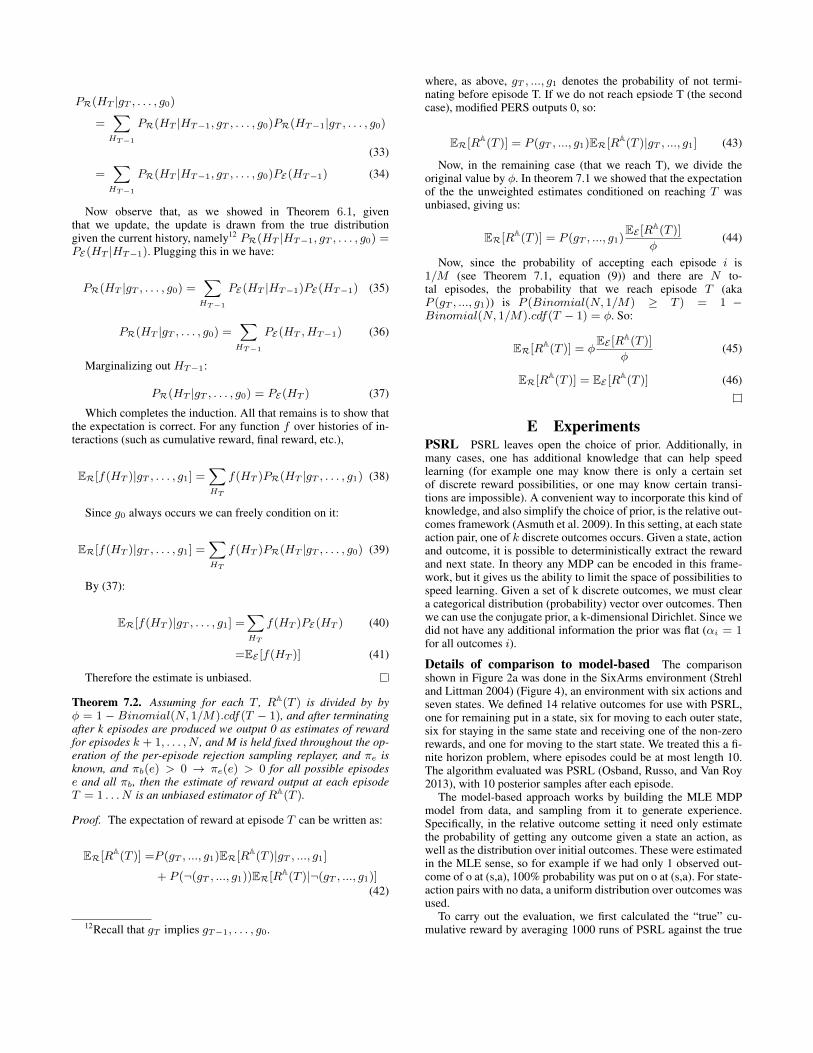
Theorem 7.2. Assuming for each T , RA(T ) is divided byby φ = 1− Binomial(N, 1/M).cdf(k − 1), and after ter-minating at timestep k we output 0 as estimates of rewardfor episodes k + 1, . . . , N , and M is held fixed throughoutthe operation of PERS, and πe is known, and πb(e) > 0 →πe(e) > 0 for all possible episodes e and all πb, then theestimate of reward output at each episode T = 1 . . . N is anunbiased estimator of RA(T ).
Proof Sketch. Outputting an estimate of the reward at anepisode T by either dividing the observed reward by theprobability of reaching T (aka P (gT , ..., g1)), for a run ofthe evaluator that reaches at least T episodes, or else out-putting a 0 if the evaluation has terminated, is an importanceweighting technique that ensures the expectation is correct.
8 ExperimentsAny RL algorithm could potentially be run with these eval-uators. Here, we show results evaluating Posterior SamplingReinforcement Learning (PSRL) (Osband et al. 2013, Strens2000), which has shown good empirical and theoretical per-formance in the finite horizon case. The standard version ofPSRL creates one deterministic policy each episode basedon a single posterior sample; however, we can sample theposterior multiple times to create multiple policies and ran-domly choose between them at each step, which allows us totest our evaluators with more or less revealed randomness.
Comparison to a model-based approach We firstcompare PSRS to a model-based approach on SixArms(Strehl and Littman 2004), a small MDP environment.Our goal is to evaluate the cumulative reward of PSRLrun with 10 posterior samples, given a dataset of 100samples collected using a uniform sampling policy.The model-based approach uses the dataset to build anMLE MDP model. Mean squared error was computedagainst the average of 1000 runs against the true en-vironment. For details see the appendix (available athttp://grail.cs.washington.edu/projects/nonstationaryeval).In Figure 2a we see that the model-based approach startsfairly accurate but quickly begins returning very poorestimates. In this setting, the estimates it returned indicatedthat PSRL was learning much more quickly than it would inreality. In contrast, our PSRS approach returns much moreaccurate estimates and ceases evaluation instead of issuingpoor estimates.

0 10 20 30 40 50Episodes
0.0
0.2
0.4
0.6
0.8
1.0M
ean S
quare
d E
rror
1e7
PSRSModel
(a) PSRS tends to be much more ac-curate than a model-based approach.
0 50 100 150 200 250 300Number of episodes per run
0
5
10
15
20
25
30
35
40
45
Perc
ent
of
runs
Queue
PSRS
PERS
Fixed-M PERS
(b) Comparing on Treefrog Treasure with3 timesteps and 1 PSRL posterior sample.
0 500 1000 1500 2000 2500Number of episodes per run
0
10
20
30
40
50
60
70
Perc
ent
of
runs
Queue
PSRS
PERS
Fixed-M PERS
(c) Comparing on Treefrog with 3timesteps and 10 PSRL posterior samples.
Figure 2: Experimental results.
Figure 3: Treefrog Treasure: players guide a frog through adynamic world, solving number line problems.
Length Results All three of our estimators produce sam-ples from the correct distribution at every step. However,they may provide different length trajectories before termi-nation. To understand the data-efficiency of each evaluator,we tested them on a real-world educational game dataset, aswell as a small but well-known MDP example.
Treefrog Treasure is an educational fractions game (Fig-ure 3). The player controls a frog to navigate levels andjump through numberlines. We have 11 actions which con-trol parameters of the numberlines. Our reward is basedon whether students learn (based on pretest-to-postest im-provement) and whether they remain engaged (measuredby whether the student quit before the posttest). We useda state space consisting of the history of actions andwhether or not the student took more than 4 tries to passa numberline (note that this space grows exponentiallywith the horizon). We varied the considered horizon be-tween 3 and 4 in our experiments. We collected a datasetof 11,550 players collected from a child-focused educa-tional website, collected using a semi-uniform samplingpolicy. More complete descriptions of the game, exper-imental methodology, method of calculating M, and de-tails of PSRL can be found in the appendix (available athttp://grail.cs.washington.edu/projects/nonstationaryeval).
Figure 2 shows results on Treefrog Treasure, with his-tograms over 100 complete runs of each evaluator. Thegraphs show how many episodes the estimator could evalu-ate the RL algorithm for, with more being better. PERS doesslightly better in a short-horizon deterministic setting (Fig-ure 2b). Increasing the posterior samples greatly improvesperformance of rejection sampling methods (Figure 2c).
We also examined an increased horizon of4 (graphs provided in appendix, available athttp://grail.cs.washington.edu/projects/nonstationaryeval).Given deterministic policies on this larger state space, allthree methods are more or less indistinguishable; however,revealing more randomness causes PERS to overtake PSRS(mean 260.54 vs. 173.52). As an extreme case, we also trieda random policy: this large amount of revealed randomnessbenefits the rejection sampling methods, especially PERS,which evaluates for much longer than the other approaches.PERS outperforms PSRS here because there are smalldifferences between the random candidate policy and thesemi-random sampling policy, and thus if PSRS enters astate with little data it is likely to terminate.
The fixed-M PERS method does much worse than thestandard version, typically barely accepting any episodes,with notable exceptions when the horizon is short (Figure2b). Since it does not adjust M it cannot take advantage ofrevealed randomness (Figure 2c). However, we still feel thatthis approach can be useful when one desires truly unbiasedestimates, and when the horizon is short. Finally, we alsonote that PERS tends to have the lowest variance, whichmakes it an attractive approach since to reduce bias oneneeds to have a high percentage of runs terminating afterthe desired length.
The state space used in Treefrog Treasure grows expo-nentially with the horizon. To examine a contrasting casewith a small state space (6 states), but a long horizon (20),we also test our approaches in Riverswim (Osband, Russo,and Van Roy 2013), a standard toy MDP environment.The results can be found in the appendix (available athttp://grail.cs.washington.edu/projects/nonstationaryeval),but in general we found that PERS and its variants suffergreatly from the long horizon, while Queue and PSRS

do much better, with PSRS doing particularly well ifrandomness is revealed.
Our conclusion is that the PERS does quite well, espe-cially if randomness is revealed and the horizon is short. Itappears there is little reason to choose Queue over PSRS,except if the sampling distribution is unknown. This is sur-prising because it conflicts with the results of Mandel et al.2015. They found a queue-based approach to be more effi-cient than rejection sampling in a non-contextual bandit set-ting, since data remained in the queues for future use insteadof being rejected. The key difference is that in bandits thereis only one state, so we do not encounter the problem thatwe happen to land on an undersampled state, hit an emptyqueue by chance, and have to terminate the whole evaluationprocedure. If the candidate policy behaves randomly at un-visited states, as is the case with 10-sample PSRL, PSRS canmitigate this problem by recognizing the similarity betweensampling and candidate distributions to accept the samplesat that state, therefore being much less likely to terminateevaluation when a sparsely-visited state is encountered.
9 ConclusionWe have developed three novel approaches for evaluatinghow RL algorithms perform online: the most important dif-ferences are summarized in Table 1. All methods have guar-antees that, given some history, if a sample is output it comesfrom the true distribution. Further, we developed a variantof PERS with even stronger guarantees of unbiasedness.Empirically, there are a variety of tradeoffs to navigate be-tween the methods, based on horizon, revealed randomnessin the candidate algorithm, and state space size. We antici-pate these approaches will find wide use when one wishesto compare different reinforcement learning algorithms ona real-world problem before deployment. Further, we areexcited at the possibility of using these approaches to cre-ate real-world testbeds for reinforcement learning problems,perhaps even leading to RL competitions similar to thosewhich related contextual bandit evaluation work (Li et al.2011) enabled in that setting (Chou and Lin 2012). Futuretheoretical work includes analyzing the sample complexityof our approaches and deriving tight deviation bounds on thereturned estimates. Another interesting direction is develop-ing more accurate estimators, e.g. by using doubly-robustestimation techniques (Dudık et al. 2012).
Acknowledgments This work was supported by the NSF BIG-DATA grant No. DGE-1546510, the Office of Naval Research grantN00014-12-C-0158, the Bill and Melinda Gates Foundation grantOPP1031488, the Hewlett Foundation grant 2012-8161, Adobe,Google, and Microsoft.
AppendixA Algorithm Details
Queue Based Evaluation: Termination UponEmpty QueueOne question raised by the queue-based method is why do we ter-minate as soon as we hit an empty stream (meaning, run out of(r, s′) tuples at the current (s, a))? Especially in an episodic set-ting, why not just throw away the episode, and start a new episode?
The reason is that this would no longer draw samples from the trueenvironment. To see why, imagine that after starting in sI , half thetime the agent goes to s1, otherwise it goes to s2. The candidatealgorithm A picks action 1 in s1, but the sampling policy avoids it99% of the time. In s2, both sampling and candidate approachespick each action with equal probability. If we run a “restart if nodata” approach, it is very unlikely to ever include a transition fromsI to s1, since there aren’t many episodes going through s1 thatpicked the action we chose, causing us to quickly run out of data.So the algorithm will almost always be fed s2 after sI , leading tothe incorrect distribution of states. Our approach does not have thisproblem, since in this case it will stop as soon as it hits a lack ofdata at s2, leading to a balanced number of samples. However, adownside of this approach is that with very large spaces, we maynot be able to produce long sequences of interactions, since in thesescenarios we may very quickly run into an empty queue.
Calculating M for PERS
Algorithm 4 Efficient M calculation
1: Input: Candidate policy πb, Exploration policy πe, com-mon state space S,
2: Binary transition matrix T denoting whether a nonzerotransition probability from s and s′ is possible a priori,maximum horizon H .
3: Initialize Ms = 1.0 for all s ∈ S4: for t = 1 to H do5: for s ∈ S do6: M ′s = maxa
πb(s,a)πe(s,a)maxs′T (s, a, s
′)Ms′
7: M =M ′
8: return MsI
Let πb(e) be shorthand for Πl(e)t=0πb(at|ht), and similarly for
πe(e)In order to ensure that rejection sampling returns a sample from
the candidate distribution, it is critical that M be set correctly.One way to understand the necessity of M is to consider thatsince the ratio πb(e)
πe(e)can grow extremely large, we need an M
such that πb(e)Mπe(e)
is a probability between 0 and 1. Therefore,
M ≥ maxeπb(e)πe(e)
Obviously, taking the maximum over all pos-sible episodes is a bit worrisome from a computational standpoint,although in some domains it may be feasible. Alternatively, onecan always use an overestimate. Some examples that may be usefulare: maxT
maxes.t.l(e)=T πb(e)
mines.st.l(e)=T πe(e)or maxe πb(e)
mine πe(e)or even 1.0
mine πe(e).
However, one needs to be careful that the overestimate is not tooextreme, or else rejection sampling will accept very few samples,since an overly large M lowers all probabilities (for example, dou-bling M means all probabilities will be normalized to [0,0.5]).
In certain cases, even if we are not willing to assume a statespace for the purposes of evaluation, we know that πb uses a dis-crete state space S1 and πe uses a discrete state space S2 . In thiscase we can formulate a common state space, either as a cross prod-uct of the two spaces or by observing that one is contained withinthe other, which allows us to avoid an exponential enumeration ofhistories as follows. Assume A does make use of additional inter-nal randomness over the course of a single episode, and the horizonis upper bounded, and we have access to a binary transition matrixT denoting whether a nonzero transition probability from s and s′
is possible a priori. Then the maximum from an episode starting ateach state Ms, satisfies the following recursion:

Ms,0 = 1.0
Ms,t = maxaπb(s, a)
πe(s, a)maxs′T (s, a, s′)Ms′,t−1
One can use a dynamic programming approach to efficientlysolve this recurrence. See algorithm 4.
PSRS: Self-Idempotent or Not?If we randomize the data in our streams and use PSRS, scenariossuch as the following can occur. Imagine we have three states, s1,s2, and s3, and a candidate policy that is identical to the samplingpolicy, so that rejection sampling accepts samples with probability1. In our initial dataset, assume we took 1 transition from s1 tos2, N transitions from s2 to s2, and one transition from s2 to s3.If we keep the order fixed, the trace will accept every transition inthe order they occurred and thus behave exactly the same as thesampling policy, accepting all data. But, if we randomize the order,as will happen in general, we are very likely to spend less than Ntransitions in s2 before we draw the tuple fromQ[s2] that causes usto transition to s3, leaving the remaining samples at s2 uncollected.
B Sample from True DistributionGuarantees
Properties of Rejection SamplingRejection sampling is guaranteed to return a sample from p(x)given an infinite stream of samples from q(x). However, in prac-tice we only have a finite stream of size N and would like to knowwhether, conditioned on the fact that rejection sampling outputs anestimate before consuming the dataset, the accepted sample is dis-tributed according to p(x). Or formally,Lemma 1. PR(x = a|r1 ∨ · · · ∨ rN ) = PE(a), where PR de-notes the probability (or pdf) under rejection sampling, PE denotesthe probability under the candidate distribution, and ri means allsamples before the ith are rejected, and x is accepted on the ith
sample.
Proof. Proof by induction on N. The base case (N=0) is triv-ial because we never return an estimate given zero data. AssumePR(x = a|r1 ∨ · · · ∨ rN−1) = PE(x = a) and show for N .
PR(x = a|r1 ∨ . . . ∨ rN )
= PR(rN )PR(x = a|rN )
+ (1− PR(rN ))PR(x = a|r1 ∨ · · · ∨ rN−1)
By the inductive hypothesis we have:
PR(x = a|r1 ∨ · · · ∨ rN )
= PR(rN )PR(x = a|rN ) + (1− PR(rN ))PE(x = a)
So it suffices to show PR(x = a|rN ) = PE(x = a).
PR(x = a|rN ) =PR(x = a, rN )
PR(rN )
PR(x = a|rN ) =PR(x = a, rN )∑b PR(x = b, rN )
Since we perform rejection sampling:
=q(a) PE(a)
Mq(a)∑b q(b)
PE(b)Mq(b)
where q is the sampling distribution.
=PE(a)M∑
bPE(b)M
=PE(a)M1M
=MPE(a)
M
= PE(a)
A note on the base caseNote that our guarantees say that, if our evaluators do not terminate,our the produced pair of tuple (or episode) and χ comes from thecorrect distribution given some history. However, these guaranteesdoes not explicitly address how the initial historyH0 is chosen. Thefollowing lemma (with trivial proof) addresses this issue explicitly:
Lemma 2. Under evaluators Queue, PSRS, and PERS,PR(H0) =PE(H0).
Proof. For all of our evaluators, the initial state is correctly ini-tialized to sI , and the initial χ is drawn correctly according to A,so the initial history H0 (consisting of initial state and initial χ) isdrawn from the correct distribution.
Queue-based evaluator guaranteesTheorem 4.1. Assuming the environment is an MDP with statespace S and the randomness involved in drawing from πb istreated as internal to A, given any history of interactions HT , ifthe queue-based evaluator produces a (s, a, r, s′) tuple, the dis-tribution of this tuple and subsequent internal randomness χ un-der the queue-based evaluator is identical to the true distributionthe agent would have encountered if it was run online. That is,PR(s, a, r, s′, χ|HT , gT ) = PE(s, a, r, s
′, χ|HT ), which gives usthat PR(HT+1|HT , gT ) = PE(HT+1|HT ).
Proof. Recall that for the queue-based evaluator we treat the ran-domness involved in drawing an action from the distribution πbas part of the χ stored in the history. Therefore, given HT (whichincludes χ), A deterministically selects aT given HT . Given anMDP and the history of interactions HT at timestep t, and as-suming for convenience s−1 = sI , PE(s, a, r, s′|HT ) = I(s =s′t−1, a = at)PE(r, s
′|s, a), where the conditional independencesfollow from the fact that in an MDP, the distribution of (r, s′) onlydepends on s, a. Under our evaluator, PR(s, a, r, s′|HT , gT ) =I(s = s′t−1, a = aT )PR(Q[s, a].pop() = (r, s′)), since the stateis properly translated from one step to the next, and the actiona is fixed to aT . So we just need to show PR(Q[s, a].pop() =(r, s′)) = PE(r, s
′|s, a). But since the (r, s′) tuple at the frontof our Q[s, a] was drawn from the true distribution9 given s, a,but independent of the samples in our history, it follows im-mediately that PR(Q[s, a].pop() = (r, s′)) = PE(r, s
′|s, a),and thus PR(s, a, r, s′|HT , gT ) = PE(s, a, r, s
′|HT ). Givenan (s, a, r, s′), the algorithm’s internal randomness χ is drawnfrom the correct distribution and thus PR(s, a, r, s′, χ|HT , gT ) =PE(s, a, r, s
′, χ|HT ).
9For further discussion of this property of queues see Joulani,Gyorgy, and Szepesvari 2013

Per-state RS evaluator GuaranteesTheorem 5.1. Assume the environment is an MDP with state spaceS, πe is known, and and for all a, πe(a) > 0 if πb(a) > 0.Then if the evaluator produces a (s, a, r, s′) tuple, the distribu-tion of (s, a, r, s′) tuple returned by PSRS (and subsequent inter-nal randomness χ) given any history of interactions HT is iden-tical to the true distribution the agent would have encounteredif was run online. Precisely, in the case that we accept a tuple,PR(s, a, r, s′, χ|HT ) = PE(s, a, r, s
′, χ|HT ), which gives us thatPR(HT+1|HT ) = PE(HT+1|HT ).
Proof. Note that the candidate distribution πb is deterministicallyoutput given HT , since HT includes any internal randomness χ bydefinition.
Given some HT at timestep T , and assuming for conveniences−1 is a fixed start state, we know s = s′t−1. So, we accept each(a, r, s′) tuple with probability:
πb(a|s)M ∗ πe(a|s)
where M = maxaπb(a|s)πe(a|s) always. Equivalently, we can say we
accept each tuple with probability:
πb(a|s)PE(r, s′|s, a)
M ∗ πe(a|s)PE(r, s′|s, a)
Let Pexplore denote the probability in the true environment un-der the sampling policy. Then we have the probability of acceptingthis tuple is:
PE(a, r, s′|s,HT )
M ∗ Pexplore(a, r, s′|s)where the conditioning on HT is introduced because the specificπb chosen depends on HT . We can write M = maxa
πb(a|s)πe(a|s) =
maxa,r,s′πb(a|s)πe(a|s) = maxa,r,s′
πb(a|s)PE (r,s′|s,a)πe(a|s)PE (r,s′|s,a)
=
maxa,r,s′PE (a,r,s
′|s,HT )Pexplore(a,r,s
′|s) . The (a, r, s′) tuples in each PSRS
stream Q[s] are drawn according to Pexplore(a, r, s′|s), since
the actions in each stream are drawn according to πe(a|s) and rand s′ are then drawn according to PE(r, s′|s, a) by the Markovassumption. Therefore, since we draw (a, r, s′) according toPexplore(a, r, s
′|s) but we wish to draw from PE(a, r, s′|s,HT ),
this is a straightforward application of rejection sampling. SinceM ≥ maxa,r,s′
PE (a,r,s′|s,HT )
Pexplore(a,r,s′|s) , rejection sampling guarantees
that a returned sample is sampled according to PE(a, r, s′|s,HT ),even if conditioned on only having a finite dataset (Lemma 1). Inother words, PR(a, r, s′|s,HT , gT ) = PE(a, r, s
′|s,HT ). Sincein both cases s is deterministically extracted from the last tuple ofHT , this implies PR(s, a, r, s′|HT , gT ) = PE(s, a, r, s
′|HT )Given an (s, a, r, s′), the algorithm’s internal random-
ness χ is drawn from the correct distribution and thusPR(s, a, r, s′, χ|HT , gT ) = PE(s, a, r, s
′, χ|HT ).
Per-Episode Rejection Sampling GuaranteesTheorem 6.1. Assuming πe is known, and πb(e) > 0→ πe(e) >0 for all possible episodes e and all πb, and PERS outputs anepisode e, then the distribution of e (and subsequent internal ran-domness χ) given any history of episodic interactions HT us-ing PERS is identical to the true distribution the agent wouldhave encountered if it was run online. That is, PE(e, χ|HT ) =PR(e, χ|HT , gT ), which gives us that PR(HT+1|HT , gT ) =PE(HT+1|HT ).
Proof. An episode e consists of some sequence of actions,observations and rewards o0, a0, r0, o1, a1, r1, . . . . Let χt de-note the internal randomness generated by algorithm A af-ter receiving rt and ot+1, so that χ = χ0, . . . , χl(e). Letht denote the within-episode history at time t, namely ht =o0, . . . , ot, a0, . . . , at−1, r0, . . . , rt−1, χ0, . . . , χt−1. Given HT ,for notational convenience we assume the algorithm A outputs asingle policy πb which maps ht (recall this includes any internalrandomness) to action probabilities, that is A chooses actions ac-cording to πb(at|ht). The sampling policy likewise chooses actionsaccording to πe(at|ht) (however the χ component of ht is not usedby the sampling policy). The environment generates observationsand rewards from some unknown distributionPE given the past his-tory, in other words according to PE(rt, ot+1|at, ht).10 We acceptepisodes with probability:∏l(e)
t=0 πb(at|ht)M∏l(e)t=0 πb(at|ht)
where M ≥∏l(e)
t=0 πb(at|ht)∏l(e)t=0 πe(at|ht)
always. This can also be written as:
∏l(e)t=0 πb(at|ht)PE(rt, ot+1|at, ht)PE(χt|ht, rt, ot+1, HT )
M∏l(e)t=0 πe(at|ht)PE(rt, ot+1|at, ht)PE(χt|ht, rt, ot+1, HT )
(1)Let Pexplore(e) denote the probability of episode e under the
exploration policy πe in the true environment. Then we have theprobability of accepting this episode is:
PE(e, χ|HT )
M ∗ Pexplore(e)∏l(e)t=0 PE(χt|ht, rt, ot+1, HT )
(2)
where the conditioning on HT in the numerator is introducedbecause how A updates πb depends on HT . We can write M ≥maxe
∏l(e)t=0 πb(at|ht)PE (rt,ot+1|at,ht)PE(χt|ht,rt,ot+1,HT )∏l(e)t=0 πe(at|ht)PE (rt,ot+1|at,ht)PE(χt|ht,rt,ot+1,HT )
=
maxePE (e,χ|HT )
Pexplore(e)∏l(e)
t=0 PE(χt|ht,rt,ot+1,HT ). The episodes e in
our dataset are drawn according to Pexplore(a, r, s′|s), since
the action at each timestep is drawn according to πe(at|ht),and then the next reward and observation are drawn ac-cording to PE(rt, ot+1|at, ht) by the episodic assumption.And during the operation of PERS A draws the internalrandomness χ according to the correct distribution at eachstep, PE(χt|ht, rt, ot+1, HT ). Since we draw e, χ according toPexplore(e)
∏l(e)t=0 PE(χt|ht, rt, ot+1, HT ), but wish to draw from
PE(e, χ), this is a straightforward application of rejection sam-pling. Since M ≥ maxe
PE (e,χ|HT )
Pexplore(e)∏l(e)
t=0 PE(χt|ht,rt,ot+1,HT ),
rejection sampling guarantees that any returned sample is sampledaccording to PE(e, χ|HT ), even if conditioned on only having afinite dataset (Lemma 1). So PR(e, χ|HT , gT ) = PE(e, χ|HT ).
C Empirical Performance ofImportance-Weighted Fixed-M PERS
Despite the stronger guarantees, one should be cautious about in-terpreting the empirical results generated by the variant proposedin Theorem 7.2. Although the expectation is correct, for a singlerun of the algorithm, the estimates will tend to rise above their true
10We assume whether the episode continues or not is an obser-vation, i.e. is it also drawn from an unknown distribution given thehistory.

value due to the importance weights (leading one to believe the al-gorithm is learning more than it truly is) before abruptly droppingto zero. Averaging together multiple unbiased estimates is morelikely to give a better picture of behavior.
D Unbiasedness ProofsTheorem 7.1. If M is held fixed throughout the operation of theper-episode rejection sampling replayer, πe is known, and πb(e) >0 → πe(e) > 0 for all possible episodes e and all πb, then if theevaluator outputs an estimate of some function f(HT ) at episodeT, that estimate is an unbiased estimator of f(HT ) at episode T, inother words, ER[f(HT )|gT , . . . , g1] =
∑HT
f(HT )PE(HT ) =
EE [f(HT )]. For example, if f(HT ) = RA(T ), the estimate is anunbiased estimator of RA(T ) given gT , . . . , g1.
Proof Sketch. We first show that if M is fixed, the probabilitythat each episode is accepted is constant (1/M ). This allows us toshow that whether we continue or not (gT ) is conditionally inde-pendent of HT−1. This lets us remove the conditioning on HT−1
in Theorem 6.1 to give us that PR(HT |gT ) = PE(HT ), meaningthe distribution over histories after T accepted episodes is correct,from which conditional unbiasedness is easily shown.
Proof. First, we will calculate the probability (over randomiza-tion in the dataset, algorithm, and evaluator) that we accept the ith
episode in our dataset, ei, given some HT (over some sequence Sof acceptances/rejections in the first i− 1 episodes).
P (Accept ei|HT , S) =∑e
P (ei = e)P (e is accepted |HT , S)
(3)If we let q(e) refer to the probability of the episode under the
sampling distribution,
P (Accept ei|HT , S) =∑e
q(e)P (e is accepted |HT , S) (4)
Recall that as part of Theorem 6.1 (equation (1)) we showed theper-episode rejection replayer accepted an episode with probability
∏l(e)t=0 πb(at|ht)PE(rt, ot+1|at, ht)PE(χt|ht, rt, ot+1, HT )
M∏l(e)t=0 πe(at|ht)PE(rt, ot+1|at, ht)PE(χt|ht, rt, ot+1, HT )
=
∏l(e)t=0 πb(at|ht)PE(rt, ot+1|at, ht)
M∏l(e)t=0 πe(at|ht)PE(rt, ot+1|at, ht)
=PE(e|HT )
Mq(e)
where PE(e|HT ) refers to the probability of episode e under the Agiven HT , and M denotes the normalizer, which is constant in thisvariant of the algorithm. So we have:
P (Accept ei|HT , S) =∑e
P (e sampled |HT , S)PE(e|HT )
Mq(e)
(5)
P (Accept ei|HT , S) =∑e
q(e)PE(e|HT )
Mq(e)(6)
P (Accept ei|HT , S) =1
M
∑e
PE(e|HT ) (7)
And since∑e PE(e|HT ) = 1,
P (Accept ei|HT , S) =1
M(8)
P (Accept ei|HT , S) is a constant it is independent of HT andS, so:
P (Accept ei|HT , S) = P (Accept ei) =1
M(9)
So we accept the ith episode with probability 1/M , where Mis a constant, and therefore independent of S and HT . We will nowproceed to show that since this is a constant, it does not cause anyhistories to be more likely than others, from which the unbiasedproperty will follow.
Next, we will prove by induction that PR(HT |gT , . . . , g0) =PE(HT ). Recall that HT denotes a trajectory of T episodic inter-actions, gT denotes the event that we continue11 (i.e. do not ter-minate evaluation) from time T − 1 to time T , PR(x) denotesthe probability of x under the replayer, and PE(x) denotes theprobability of x in the true (online) environment under the can-didate policy. The base case is trivial (Since g0 always occurs,PR(H0|g0) = PR(H0), and by Lemma 2, PR(H0) = PE(H0)).We now assume this holds for T − 1 and we will show it holds forT .
PR(HT |gT , . . . , g0)
=∑HT−1
PR(HT |HT−1, gT , . . . , g0)PR(HT−1|gT , . . . , g0)
(10)
Our next step is to show that gT ⊥ HT−1|gT−1, so that we canturn the right term of equation (10) into the inductive hypothesis (⊥denotes independance). Let i be the number of episodes consumedafter accepting the (T − 1)th episode, so that there are exactlyN − i episodes remaining after accepting the (T − 1)th. Since, aswe showed in equation (9), P (Accept ei) = 1
M, given gT−1 and
N − i episodes remaining, gT is drawn from a Bernoulli(1 −(1− 1
M)N−i) distribution. So, since M and N are both constants,
gT ⊥ HT−1|gT−1, i. So we can write:
P (gT , HT−1|gT−1) =∑i
P (gT , HT−1|gT−1, i)P (i|gT−1)
(11)
=∑i
P (gT |gT−1, i)P (HT−1|gT−1, i)P (i|gT−1) (12)
So we need to show HT−1 ⊥ i|gT−1.
P (HT−1, i|gT−1) =1
P (gT−1)P (HT−1, gT−1, i) (13)
Now, we know the ith episode must have been accepted, butthe (T − 2)th acceptances could have occurred anywhere in the(i − 1)th steps. The probability of the jth e, χ pair in the history,HT−1[j] being accepted on the next episode given some sequenceof previously accepted/rejected episodes S is
11Since we always generate the initial history H0, for the pur-poses of induction we here condition on g0 even though that is notstrictly necessary since it always occurs.

P (HT−1[j] produced|Hj−1, S)
= P (HT−1[j] sampled|Hj−1, S)P (HT−1[j] accepted|Hj−1, S)
= q(HT−1[j]|Hj−1)PE(HT−1[j]|Hj−1)
Mq(HT−1[j]|Hj−1),
(14)
where q(HT−1[j]|Hj−1) denotes the probabilities of producingthe jth e, χ tuple in the history given Hj−1 and sampling actionsaccording to πe, and P (HT−1[j] accepted) is derived as per equa-tion (2) in Theorem 6.1. Equation (14) can be simplified:
P (HT−1[j] produced|Hj−1, S) =PE(HT−1[j]|Hj−1)
M(15)
Note that this depends on Hj−1 but is independent of S. Theprobability of rejection given S, Hj−1 is a constant 1 − 1
M(see
equation (9)), so returning to equation 13 we have:
P (HT−1, i|gT−1) (16)
=1
P (gT−1)
∑S s.t. S compat (i, T − 1)
P (S, HT−1) (17)
where (S compat (i, T − 1)), means |S| = i, there are T − 1acceptances in S, and S[i − 1] is not a rejection. Now, com-puting P (S, HT−1) would consist of multiplying quantities likeP (reject episode k | S up to k − 1)∗ P (accept HT−1[3] on episode k+1 |H2, S up to k) ∗ . . . . Note,however, that the probability of rejecting an episode is independentof the particular past sequence of acceptances and rejections (seeequation (9)), and so is the probability of accepting the next item inthe history (see equation (15)). Therefore, for every S, P (S, HT−1)is the multiplication of the probability of the initial history P (H0)with i−T+1 rejection probabilities together with the probabilitiesof accepting the T − 1 items in the history. There are
(i−1T−2
)pos-
sible different sequences S such that (S compat (i, T − 1)), sincethe last element is always accepted. Therefore:
P (HT−1, i|gT−1)
=P (H0)
P (gT−1)
(i− 1
T − 2
)(1− 1
M)i−T+1
T−1∏j=1
PE(HT−1[j]|Hj−1)
M
(18)
since the probability of rejecting the kth episode is (1− 1M
) from(9), and from (15) the probability of accepting the jth element inthe history on the kth episode is PE (HT−1[j]|Hj−1)
M.
By Lemma 2, PR(H0) = PE(H0), so:
P (HT−1, i|gT−1)
=PE(H0)
P (gT−1)
(i− 1
T − 2
)(1− 1
M)i−T+1
T−1∏j=1
PE(HT−1[j]|Hj−1)
M
(19)
=(PE(H0)
T−1∏j=1
PE(HT−1[j]|Hj−1))1
P (gT−1)
∗
(i− 1
T − 2
)(1− 1
M)i−T+1
T−1∏j=1
1
M
(20)
Where (20) follows by simply reordering themultiplication. Now by definition, PE(HT−1) =
PE(H0)∏T−1j=1 PE(HT−1[j]|Hj−1), so we have:
P (HT−1, i|gT−1)
=PE(HT−1)1
P (gT−1)
(i− 1
T − 2
)(1− 1
M)i−T+1
T−1∏j=1
1
M
(21)
Now by induction, PE(HT−1) = PR(HT−1|gT−1), so:
P (HT−1, i|gT−1)
=P (HT−1|gT−1)1
P (gT−1)
(i− 1
T − 2
)(1− 1
M)i−T+1
T−1∏j=1
1
M
(22)
Note that(i−1T−2
)(1 − 1
M)i−T+1∏T−1
j=11M
is just the probabilityof consuming i elements and accepting exactly T − 1 of them(namely the binomial formula, where the probability of success(acceptance) is 1
M), so:
P (HT−1, i|gT−1) = P (HT−1|gT−1)P (i, gT−1)
P (gT−1)(23)
By the definition of conditional probability:
P (HT−1, i|gT−1) =P (HT−1|gT−1)P (i|gT−1) (24)
So since P (HT−1, i|gT−1) = P (HT−1|gT−1)P (i|gT−1),HT−1 ⊥ i|gT−1. Now returning to equation (12) we have:
P (gT , HT−1|gT−1)
=∑i
P (gT |gT−1, i)P (HT−1|gT−1, i)P (i|gT−1) (25)
Since HT−1 ⊥ i|gT−1:
P (gT , HT−1|gT−1) (26)
=∑i
P (gT |gT−1, i)P (HT−1|gT−1)P (i|gT−1) (27)
=P (HT−1|gT−1)∑i
P (gT |gT−1, i)P (i|gT−1) (28)
=P (HT−1|gT−1)∑i
P (gT , gT−1, i)
P (i, gT−1)
P (i, gT−1)
P (gT−1)(29)
=P (HT−1|gT−1)
∑i P (gT , gT−1, i)
P (gT−1)(30)
=P (HT−1|gT−1)P (gT , gT−1)
P (gT−1)(31)
=P (HT−1|gT−1)P (gT |gT−1) (32)
Where equation (31) follows since i is marginalized out, and(32) follows by the definition of conditional probability. So equa-tion (32) tells us that gT ⊥ HT−1|gT−1.
Given this conditional independence,PR(HT−1|gT , gT−1, . . . , g1) = PR(HT−1|gT−1, . . . , g0),and PR(HT−1|gT−1, . . . , g0) = PE(HT−1) by induction. SoPR(HT−1|gT , . . . , g0) = PE(HT−1). Therefore, picking upfrom (10), we have:
PR(HT |gT , . . . , g0)
=∑HT−1
PR(HT |HT−1, gT , . . . , g0)PR(HT−1|gT , . . . , g0)
(33)
=∑HT−1
PR(HT |HT−1, gT , . . . , g0)PE(HT−1) (34)
Now observe that, as we showed in Theorem 6.1, giventhat we update, the update is drawn from the true distributiongiven the current history, namely12 PR(HT |HT−1, gT , . . . , g0) =PE(HT |HT−1). Plugging this in we have:
PR(HT |gT , . . . , g0) =∑HT−1
PE(HT |HT−1)PE(HT−1) (35)
PR(HT |gT , . . . , g0) =∑HT−1
PE(HT , HT−1) (36)
Marginalizing out HT−1:
PR(HT |gT , . . . , g0) = PE(HT ) (37)
Which completes the induction. All that remains is to show thatthe expectation is correct. For any function f over histories of in-teractions (such as cumulative reward, final reward, etc.),
ER[f(HT )|gT , . . . , g1] =∑HT
f(HT )PR(HT |gT , . . . , g1) (38)
Since g0 always occurs we can freely condition on it:
ER[f(HT )|gT , . . . , g1] =∑HT
f(HT )PR(HT |gT , . . . , g0) (39)
By (37):
ER[f(HT )|gT , . . . , g1] =∑HT
f(HT )PE(HT ) (40)
=EE [f(HT )] (41)
Therefore the estimate is unbiased.
Theorem 7.2. Assuming for each T , RA(T ) is divided by byφ = 1 − Binomial(N, 1/M).cdf(T − 1), and after terminatingafter k episodes are produced we output 0 as estimates of rewardfor episodes k + 1, . . . , N , and M is held fixed throughout the op-eration of the per-episode rejection sampling replayer, and πe isknown, and πb(e) > 0 → πe(e) > 0 for all possible episodese and all πb, then the estimate of reward output at each episodeT = 1 . . . N is an unbiased estimator of RA(T ).
Proof. The expectation of reward at episode T can be written as:
ER[RA(T )] =P (gT , ..., g1)ER[RA(T )|gT , ..., g1]
+ P (¬(gT , ..., g1))ER[RA(T )|¬(gT , ..., g1)](42)
12Recall that gT implies gT−1, . . . , g0.
where, as above, gT , ..., g1 denotes the probability of not termi-nating before episode T. If we do not reach epsiode T (the secondcase), modified PERS outputs 0, so:
ER[RA(T )] = P (gT , ..., g1)ER[RA(T )|gT , ..., g1] (43)
Now, in the remaining case (that we reach T), we divide theoriginal value by φ. In theorem 7.1 we showed that the expectationof the the unweighted estimates conditioned on reaching T wasunbiased, giving us:
ER[RA(T )] = P (gT , ..., g1)EE [RA(T )]
φ(44)
Now, since the probability of accepting each episode i is1/M (see Theorem 7.1, equation (9)) and there are N to-tal episodes, the probability that we reach episode T (akaP (gT , ..., g1)) is P (Binomial(N, 1/M) ≥ T ) = 1 −Binomial(N, 1/M).cdf(T − 1) = φ. So:
ER[RA(T )] = φEE [RA(T )]
φ(45)
ER[RA(T )] = EE [RA(T )] (46)
E ExperimentsPSRL PSRL leaves open the choice of prior. Additionally, inmany cases, one has additional knowledge that can help speedlearning (for example one may know there is only a certain setof discrete reward possibilities, or one may know certain transi-tions are impossible). A convenient way to incorporate this kind ofknowledge, and also simplify the choice of prior, is the relative out-comes framework (Asmuth et al. 2009). In this setting, at each stateaction pair, one of k discrete outcomes occurs. Given a state, actionand outcome, it is possible to deterministically extract the rewardand next state. In theory any MDP can be encoded in this frame-work, but it gives us the ability to limit the space of possibilities tospeed learning. Given a set of k discrete outcomes, we must cleara categorical distribution (probability) vector over outcomes. Thenwe can use the conjugate prior, a k-dimensional Dirichlet. Since wedid not have any additional information the prior was flat (αi = 1for all outcomes i).
Details of comparison to model-based The comparisonshown in Figure 2a was done in the SixArms environment (Strehland Littman 2004) (Figure 4), an environment with six actions andseven states. We defined 14 relative outcomes for use with PSRL,one for remaining put in a state, six for moving to each outer state,six for staying in the same state and receiving one of the non-zerorewards, and one for moving to the start state. We treated this a fi-nite horizon problem, where episodes could be at most length 10.The algorithm evaluated was PSRL (Osband, Russo, and Van Roy2013), with 10 posterior samples after each episode.
The model-based approach works by building the MLE MDPmodel from data, and sampling from it to generate experience.Specifically, in the relative outcome setting it need only estimatethe probability of getting any outcome given a state an action, aswell as the distribution over initial outcomes. These were estimatedin the MLE sense, so for example if we had only 1 observed out-come of o at (s,a), 100% probability was put on o at (s,a). For state-action pairs with no data, a uniform distribution over outcomes wasused.
To carry out the evaluation, we first calculated the “true” cu-mulative reward by averaging 1000 runs of PSRL against the true

Figure 4: The SixArms environment. The labels on eachedge are (a, p, r) tuples, where p is the probability of tak-ing that transition. Image taken from Strehl et al. 2004.
environment. Then, for each evaluator (PSRS and model-based) wesampled 100 different datasets of 100 episodes from SixArms us-ing a uniform sampling policy. We then ran 10 complete runs ofthe evaluator on that dataset, each of which returned estimates ofcumulative reward. For PSRS, we only reported estimates up to theminimum evaluation length across those ten runs13. The squarederror was computed between the mean of the 10 runs and the truecumulative reward curve. Finally, to compute the MSE, the averageover the 100 runs was taken (ignoring cases where no estimate wasreturned).
Treefrog Treasure Experiment Setup Treefrog Treasure isan educational fractions game (Figure 3). The player controls a frogto navigate levels and jump through numberlines. Our action set isdefined as follows: After giving an in-game pretest we give a firstset of lines, then we want to either increase the difficulty level ofone parameter (e.g. removing tick marks), stay, or go back, whichwe encoded as 11 actions. Our reward is terminal and ranges from-2 to 4. It measures engagement (measured by whether the stu-dent quit before the posttest) and learning (measured by pretest-to-posttest improvement). After each step we additionally receivea binary observation informing us whether the student took morethan 4 attempts on the last pair of lines. The relative outcomes de-fined for PSRL included either terminating with some reward (-2 -4) or continuing with one of the two observations. We used a statespace consisting of the history of actions and the last observation.The true horizon is 5, but for reasons of data sparsity (induced by alarge action space and thus large state space) we varied the horizonbetween 3 and 4 in our experiments.
Our dataset of 11,550 players was collected from Brain-POP.com, an educational website focused on school-aged children.The sampling policy used was semi-uniform and changed fromday-to-day. We logged the probabilities for use with the rejection-sampling evaluator, modifying the rejection sampling approachesslightly to recalculate M at every step based on the changing sam-pling policy.
For PERS we use14 Algorithm 4 to calculate M , updating itbased both on the change in the algorithm and the change in the
13This was following the approach proposed in (Mandel et al.2015) to mitigate the bias introduced by having a wide variance inevaluation lengths, a problem we discuss in section 7.
14With straightforward extensions to handle policies that dependon both s and t.
sampling policy. We also tried a variant which fixed M so as toachieve the unbiasedness guarantees in Theorem 7.1. To calculatethis M we upper bounded the probability of an episode under ourcandidate distribution by 1, and calculated the minimum probabil-ity our sampling distribution could place on any episode.15
Further Treefrog Treasure Results We also examined anincreased horizon of 4. Given deterministic policies on this largerstate space, all three methods are more or less indistinguishable(Figure 5a) ; however, revealing more randomness causes PERSto overtake PSRS (mean 260.54 vs. 173.52), Figure 5b). As anextreme case, we also tried a random policy in Figure 5c: thislarge amount of revealed randomness benefits the rejection sam-pling methods, especially PERS, who evaluates for much longerthan the other approaches. PERS outperforms PSRS here becausethere are small differences between the random candidate policyand the semi-random sampling policy, and thus if PSRS enters astate with little data it is likely to terminate.
Riverswim RiverSwim is described in Figure 6a.In this domain we defined a space of 5 relative out-comes: {MovedRight, MovedLeft, Staywith0reward, Stay-with5/1000reward,Staywith1reward}. To generate histograms over100 sizes, for each evaluator we sampled 10 datasets of 10000episodes from this MDP, using a uniform sampling policy, andused each dataset for 10 runs of evaluation.
The results with 10-sample PSRL are shown in figure 6b.The per-episode rejection sampler was only able to accept a fewepisodes due to their length, while the two state-based evaluatorsleveraged the known state space to accept a substantially largernumber of episodes. To more clearly understand sensitivity to re-vealed randomness, we tested two versions of a random policy:one which revealed its randomness and one which did not. In thecase where the randomness was hidden (Figure 6c), we see that theper-episode rejection sampling approach does so poorly it never ac-cepts any episodes and thus is hard to see on the graph, the per-staterejection sampling has fairly mediocre performance, and the queue-based method does the best. This is because the per-state rejectionsampler, by treating the data as a stream, discards a lot of data forarms it did not choose to pull, unlike the queue-based approachwhich only discards data when it is consumed by the algorithm.We suspect the effect is particularly visible here for two reasons:(a) There are a small number of states, making it more similar to thebandit case where Queue does well (Mandel et al. 2015) and (b) thepolicy is not explicitly driving exploration towards poorly-visitedstates, which often causes both state-based methods to fail fairlyquickly. When the randomness is revealed (Figure 6d), the two re-jection sampling approaches improve greatly in performance. Onecan observe how the per-episode version is self-idempotent (sincethe sampling policy was the same as the candidate policy, all 10,000episodes were accepted) while the per-state is not.
ReferencesAsmuth, J.; Li, L.; Littman, M. L.; Nouri, A.; and Wingate, D.2009. A bayesian sampling approach to exploration in reinforce-ment learning. In Proceedings of the Twenty-Fifth Conference onUncertainty in Artificial Intelligence, 19–26. AUAI Press.
15This is probably fairly close to the minimum fixed M , sincePSRL randomly generates distributions by sampling N times fromthe posterior, and we have to consider the worst case over that ran-domization, which always has a small probability of placing prob-ability 1 on the minimum-probability episode under the samplingdistribution.
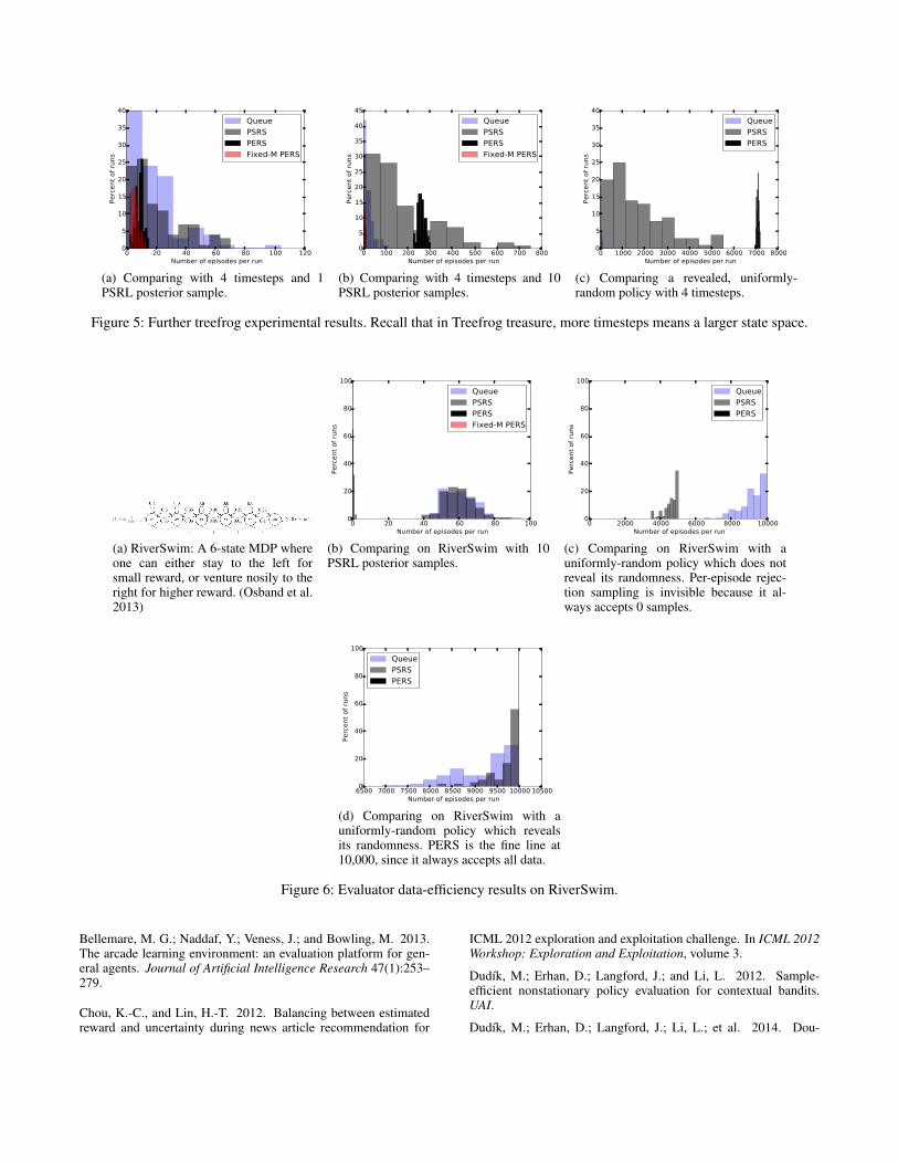
0 20 40 60 80 100 120Number of episodes per run
0
5
10
15
20
25
30
35
40Perc
ent
of
runs
Queue
PSRS
PERS
Fixed-M PERS
(a) Comparing with 4 timesteps and 1PSRL posterior sample.
0 100 200 300 400 500 600 700 800Number of episodes per run
0
5
10
15
20
25
30
35
40
45
Perc
ent
of
runs
Queue
PSRS
PERS
Fixed-M PERS
(b) Comparing with 4 timesteps and 10PSRL posterior samples.
0 1000 2000 3000 4000 5000 6000 7000 8000Number of episodes per run
0
5
10
15
20
25
30
35
40
Perc
ent
of
runs
Queue
PSRS
PERS
(c) Comparing a revealed, uniformly-random policy with 4 timesteps.
Figure 5: Further treefrog experimental results. Recall that in Treefrog treasure, more timesteps means a larger state space.
(a) RiverSwim: A 6-state MDP whereone can either stay to the left forsmall reward, or venture nosily to theright for higher reward. (Osband et al.2013)
0 20 40 60 80 100Number of episodes per run
0
20
40
60
80
100
Perc
ent
of
runs
Queue
PSRS
PERS
Fixed-M PERS
(b) Comparing on RiverSwim with 10PSRL posterior samples.
0 2000 4000 6000 8000 10000Number of episodes per run
0
20
40
60
80
100
Perc
ent
of
runs
Queue
PSRS
PERS
(c) Comparing on RiverSwim with auniformly-random policy which does notreveal its randomness. Per-episode rejec-tion sampling is invisible because it al-ways accepts 0 samples.
6500 7000 7500 8000 8500 9000 9500 10000 10500Number of episodes per run
0
20
40
60
80
100
Perc
ent
of
runs
Queue
PSRS
PERS
(d) Comparing on RiverSwim with auniformly-random policy which revealsits randomness. PERS is the fine line at10,000, since it always accepts all data.
Figure 6: Evaluator data-efficiency results on RiverSwim.
Bellemare, M. G.; Naddaf, Y.; Veness, J.; and Bowling, M. 2013.The arcade learning environment: an evaluation platform for gen-eral agents. Journal of Artificial Intelligence Research 47(1):253–279.
Chou, K.-C., and Lin, H.-T. 2012. Balancing between estimatedreward and uncertainty during news article recommendation for
ICML 2012 exploration and exploitation challenge. In ICML 2012Workshop: Exploration and Exploitation, volume 3.
Dudık, M.; Erhan, D.; Langford, J.; and Li, L. 2012. Sample-efficient nonstationary policy evaluation for contextual bandits.UAI.
Dudık, M.; Erhan, D.; Langford, J.; Li, L.; et al. 2014. Dou-

bly robust policy evaluation and optimization. Statistical Science29(4):485–511.Fonteneau, R.; Murphy, S.; Wehenkel, L.; and Ernst, D. 2010.Model-free monte carlo-like policy evaluation. In Thirteenth Inter-national Conference on Artificial Intelligence and Statistics (AIS-TATS 2010).Fonteneau, R.; Murphy, S. A.; Wehenkel, L.; and Ernst, D. 2013.Batch mode reinforcement learning based on the synthesis of arti-ficial trajectories. Annals of operations research 208(1):383–416.Gelman, A.; Carlin, J. B.; Stern, H. S.; and Rubin, D. B. 2014.Bayesian data analysis, volume 2. Taylor & Francis.Joulani, P.; Gyorgy, A.; and Szepesvari, C. 2013. Online learningunder delayed feedback. In Proceedings of The 30th InternationalConference on Machine Learning, 1453–1461.Levine, S., and Koltun, V. 2013. Guided policy search. In Proceed-ings of The 30th International Conference on Machine Learning,1–9.Li, L.; Chu, W.; Langford, J.; and Wang, X. 2011. Unbiased of-fline evaluation of contextual-bandit-based news article recommen-dation algorithms. In WSDM, 297–306. ACM.Maei, H. R., and Sutton, R. S. 2010. GQ (λ): A general gradientalgorithm for temporal-difference prediction learning with eligibil-ity traces. In Proceedings of the Third Conference on ArtificialGeneral Intelligence, volume 1, 91–96.Mahmood, A. R.; van Hasselt, H. P.; and Sutton, R. S. 2014.Weighted importance sampling for off-policy learning with linearfunction approximation. In Advances in Neural Information Pro-cessing Systems, 3014–3022.Mandel, T.; Liu, Y.-E.; Levine, S.; Brunskill, E.; and Popovic, Z.2014. Offline policy evaluation across representations with appli-cations to educational games. In AAMAS, 1077–1084. IFAAMAS.Mandel, T.; Liu, Y.-E.; Brunskill, E.; and Popovic, Z. 2015. Thequeue method: Handling delay, heuristics, prior data, and evalua-tion in bandits. AAAI.Mary, J.; Preux, P.; and Nicol, O. 2014. Improving offline evalua-tion of contextual bandit algorithms via bootstrapping techniques.In Proceedings of the 31st International Conference on MachineLearning (ICML-14), 172–180.Osband, I.; Russo, D.; and Van Roy, B. 2013. (More) efficient rein-forcement learning via posterior sampling. In Advances in NeuralInformation Processing Systems, 3003–3011.Peshkin, L., and Shelton, C. R. 2002. Learning from scarce expe-rience. ICML.Precup, D. 2000. Eligibility traces for off-policy policy evaluation.Computer Science Department Faculty Publication Series 80.Ross, S.; Gordon, G. J.; and Bagnell, J. A. 2011. A reductionof imitation learning and structured prediction to no-regret onlinelearning. AISTATS.Strehl, A. L., and Littman, M. L. 2004. An empirical evaluationof interval estimation for Markov decision processes. In Tools withArtificial Intelligence, 2004. ICTAI 2004. 16th IEEE InternationalConference on, 128–135. IEEE.Strens, M. 2000. A Bayesian framework for reinforcement learn-ing. In ICML, 943–950.Sutton, R. S.; Mahmood, A. R.; and White, M. 2015. An emphaticapproach to the problem of off-policy temporal-difference learning.arXiv preprint arXiv:1503.04269.Thomas, P. S.; Theocharous, G.; and Ghavamzadeh, M. 2015. Highconfidence off-policy evaluation. AAAI.