OFFICE OF INDUSTRIES WORKING PAPER U.S. … · those of the U.S. International Trade Commission ......

DYNAMIC ECONOMIC RELATIONSHIPS AMONG U.S.SOY PRODUCT MARKETS: USING A COINTEGRATED

VECTOR AUTOREGRESSION APPROACH WITHDIRECTED ACYCLIC GRAPHS

No. ID-13

OFFICE OF INDUSTRIES WORKING PAPERU.S. International Trade Commission

Ronald A. BabulaDavid A. Bessler

andRobert A. Rogowsky

September 2005

R. Babula is an Industry Economist with the Agriculture and Fisheries Division, Office ofIndustries, and R. Rogowsky is the Director of Operations, of the U.S. International TradeCommission. D. Bessler is a Professor in the Department of Agricultural Economics, TexasA.&M University, College Station, Texas. This paper’s views do not necessarily representthose of the U.S. International Trade Commission (USITC) or any of its individualCommissioners. Working papers are circulated to promote the active exchange of ideasbetween USITC staff and recognized experts outside the USITC, and to promoteprofessional development of Office staff by encouraging outside professional critique ofstaff research. The authors gratefully acknowledge the expert assistance of Ophelia McCardell, of the Office of Operations, and Phyllis Boone and Janice Wayne, both of theOffice of Industies, in preparing and formatting this paper for publication.

ADDRESS CORRESPONDENCE TO:OFFICE OF INDUSTRIES

U.S. INTERNATIONAL TRADE COMMISSIONWASHINGTON, DC 20436 USA

Dynamic Economic Relationships Among U.S. Soy Product Markets: Using a CointegratedVector Autoregression Approach with Directed Acyclic Graphs

Ronald A. Babula (U.S. International Trade Commission)

David A. Bessler (Texas A&M University)

Robert A. Rogowsky (U.S. International Trade Commission)

ABSTRACT: This paper applies a combined methodology of a recently developed directed acyclic graph(DAG) analysis with Johansen and Juselius’ methods of the cointegrated vector autoregression (VAR)model to a monthly U.S. system of markets for soybeans, soy meal, and soy oil. Primarily a methodspaper, Johansen and Juselius’ procedures are applied, with a special focus on statistically addressinginformation inherent in well-known sources of non-normal data behavior to illustrate the effectiveness ofmodeling the system as a cointegrated multi-market system. Perhaps for the first time, methods of thecointegrated VAR model are combined with DAG analysis to account for contemporaneously correlatedresiduals, and are applied to this U.S. soy-based system. Analysis of the error correction or cointegrationspace illuminates the empirical nature of policy-relevant market elasticities, price transmissionparameters, and effects of important policy and institutional changes/events on U.S. soy-related marketsat long-run horizons beyond a single crop cycle. A statistically strong U.S. demand for soybeans emergedas the primary cointegrating relation in the error-correction space. Analysis of the DAG-adjustedcointegrated VAR model’s forecast error variance decomposition illuminates how the soy-relatedvariables and the three U.S. soy product markets dynamically interact at alternative time horizonsextending up to two-years.

Key words: Directed acyclic graphs, cointegration, vector error correction and vector autoregressionmodels, monthly U.S. soy-based markets.

1 The “split” year refers to the “crop or market” year. The U.S. crop or market year begins on September 1 andends August 31 of the ensuing year, such that 2003/04 denotes September 1, 2003 – August 31, 2004. For soy mealand soy oil, the market year starts October 1 and ends September 30 of the ensuing year, such that 2003/04 denotesOctober 1, 2003 – September 30, 2004.

1

Introduction

Prices of soybeans and soy products were, until recently, at record high levels not seen since the1970s (U.S. Department of Agriculture, Economic Research Service or USDA,ERS, 2004a, b). Since abrief “grain/oilseed crisis” of high and low supplies during the mid-1990s, world grain and oilseedmarkets have been mostly quiet with low and often declining prices until 2003. However, price volatilityreturned swiftly during the 2003/04 marketing year,1 primarily because of three powerful influences (seeBabula, Bessler, Reeder, and Somwaru or BBRS 2004, p. 29). First, unfavorable weather stunted the2002 and 2003 crops in the Northern and Southern hemispheres. Second, there was an escalating Chinesedemand for grain and oilseeds for use as raw materials. And third, several serious livestock diseasesparalyzed production and trade in meat and related meat byproducts. And while soy and oilseed productprices have declined noticeably since August 2004, effects of oilseed product prices are keenly watchedand are of continued interest for these key U.S. commodities (BBRS 2004, p. 29).

We have two purposes. The first is methodological: we combine the methods of the cointegratedvector autoregression or VAR modeling with new and advanced methods of directed acyclic graphs(DAGs) in order to harness information on contemporaneously causal relationships, and apply thismethod combination to monthly U.S. markets for soybeans, soy meal, and soy oil. This may be the firstconcurrent application of the cointegrated VAR methods developed by Johansen (1988) and Johansen andJuselius (1990, 1992) and of the methods of DAG analysis of Bessler and Akleman (1998) to the three-market system of U.S. soy-based products.

Our second purpose is to then use the estimated cointegrated VAR model of the U.S. soy productcomplex mentioned above and obtain a series of policy-relevant econometric results. Such results includecrucial market parameter estimates (e.g. the U.S. price elasticity of soybean demand) from an analysis ofthe long run equilibrium relationships that emerge from the cointegration space, as well as an illuminationof the dynamic nature of how soy-based prices and quantities and soy-based markets interact. As well,we exploit the cointegration properties of the model for empirical indications on how statisticallyimportant (or unimportant) well-known institutional and policy changes such as the 1995 implementationof the North American Free Trade Agreement (NAFTA) and the 2002 implementation of the current U.S.farm bill (among other events) have influenced market-clearing prices and quantities and the dynamicinteractions of the three U.S. soy-based product markets.

This paper extends the work of Babula, Bessler, Reeder, and Somwaru (BBRS, 2004) who usedmore dated tools and tests, and uncovered evidence that justified the estimation of the same data set as alevels vector autoregression or VAR. We update the set of tools and tests used by BBRS with those ofJuselius (2004), and uncovered evidence that also justifies the estimation of BBRS’ monthly system ofU.S. soy product markets alternatively as a cointegrated VAR.

2 This unrestricted VEC is the model before one tests for cointegration, before rank is imposed on thecointegration space, and prior to the imposition of statistically supported coefficient restrictions that emerge from aseries of formal hypothesis tests. As in the literature, the cointegrated VAR model and cointegrated VEC model areterms used interchangeably throughout this study.

2

The remainder of this paper is comprised of eight sections. The first section presents a discussionof time series econometrics, VAR models, and cointegrated VEC models as ways of empiricallyexamining monthly U.S. markets for soybeans, soy meal, and soy oil. As well, the six modeled soy-basedmarket variables are presented, along with the data and data sources. A second section on data analysisexamines the model specification implications of harnessing the statistical information inherent instatistically non-normal data. It is well-known that harnessing such information inherent in non-normalbehavioral attributes is required for uncompromised inference and in some cases, unbiased regressionestimates (Granger and Newbold 1986, pp. 1-5). The third section provides specification of the system asa traditional levels-based VAR model. Following Juselius (2004, chapter 4), effort is expended onachieving an adequately specified levels VAR and its algebraic equivalent, the unrestricted VEC model.2 This section provides an analysis of results from a battery of diagnostic tests recommended in Johansenand Juselius (1990, 1992) and Juselius (2004, pp. 72-82). Fourth, Johansen and Juselius’ (1990, 1992)well-known trace tests and analysis of other relevant evidence are used to determine the reduced rank(“r”) of the cointegration space and the number of long run cointegrating relationships, and then restrictthe cointegration space for this reduced rank. Fifth, Johansen and Juselius’ well-known hypothesis testprocedures are applied to the rank-restricted cointegration space to reveal the nature of the long runrelationships tying together the upstream and downstream soy-based markets. A sixth section provides aneconomic interpretation of the cointegrating relations that are fully restricted for rank and for anystatistically-supported restrictions that emerged from the hypothesis tests on the cointegration spacecoefficients. A seventh section follows Bessler and Akleman’s methodology and applies DAG analysis tostatistically supported patterns of contemporaneous correlations among the fully restricted cointegratedVEC model’s innovations (i.e., residuals). We then provide an innovation accounting analysis of theDAG-adjusted cointegrated VEC models’ forecast error variance decompositions. These resultsilluminate the dynamic nature with which soy-based prices and quantities and soy-based markets interact. And finally, a summary and conclusions section follow.

Time Series Econometric Considerations, Modeled Markets, and Data Resources

Since Engle and Granger’s (1987) paper, it is well-known that economic time series often fail tomeet the conditions of weak stationarity summarized by Granger and Newbold (1986, pp. 1-5). Nonetheless, it is also well-known that while data series are often individually nonstationary, they canform vectors with linear combinations which are stationary, such that the vector of interrelated series are“cointegrated” and move together in tandem as an error-correcting system (Johansen and Juselius 1990,1992; Juselius 2004). These well-known econometric concepts are summarized, but not detailed here. Asdemonstrated later, readers should note that most of the modeled soy-based variables defined below arenonstationary: the non-stationary ones are integrated of order-1 or I(1), with the first differences being

3 Juselius (2004, pp. 221-223) recommends that the stationarity tests on any single time series be conducted witha chi-square-distributed likelihood ratio statistic within the concept of a modeled system where the cointegrationspace is restricted for appropriate rank, and not with such univariate tests as those of Fuller (1976) and Dickey andFuller (1979). Juselius suggests that one take a vector system suspected as cointegrated in levels; obtain anadequately specified levels VAR and equivalent unrestricted VEC; determine the rank of the system; impose theappropriate reduced rank on the cointegration space; and then test each variable’s stationarity with a chi-square value(Juselius 2004, pp. 221-223). This is equivalent to testing whether the variable forms a unit vector or a separatecointegrating relationship within the reduced-rank setting. If evidence suggests that all of the endogenous variablesare indeed stationary, then one respecifies as a levels VAR.

4 Readers should note that market clearing quantities of soy meal and soy oil (QMEAL and QOIL) are defined asmonthly sums of beginning stocks, production, and imports as production levels are available each month for soymeal and soy oil. QBEANS is defined as the monthly sum of exports, volumes crushed, and ending stocks, which isalso the market-clearing quantity. This alternative definition of market-clearing quantity was followed for QBEANSbecause monthly production figures for U.S. soybeans do not exist.

3

integrated of order-zero or I(0) and stationary.3 Six soy-based variables were endogenously modeled, ofwhich four are shown below to be I(1) and two are I(0).

All data are monthly and seasonally unadjusted. A rigorous search of monthly data resources onU.S. soy-based products rendered six variables: price and quantity for soybeans, soy meal and soy oil forthe January 1992 – September, 2004 (hereinafter, 1992:01 – 2004:09). Unfortunately, data were notavailable for periods prior to 1992. The following six variables below are those which we formulate intoan unrestricted VAR and ultimately a cointegrated VEC. All data were obtained from the U.S.Department of Agriculture, Economic Research Service (hereinafter, USDA, ERS, 2004a, 2004b) andplaced uniformly into metric ton equivalents and natural logarithms before modeling. The variabledefinitions follow those adapted in recent time series research (BBRS, 2004, pp. 31-32) and include:

1. Market-clearing quantity of soybeans (QBEANS).4

2. Farm price of soybeans (PBEANS).

3. Market-clearing quantity of soy meal (QMEAL).

4. Price of soy meal (PMEAL).

5. Market-clearing quantity of soy oil (QOIL).

6. Price of soy oil (POIL).

Analysis of the Soy-Based Time Series Data

Figures 1 through 6 provide the plotted (logged) levels of the modeled data in the upper panels,and data in the first differences of logged levels are plotted in the lower panels. A weakly stationaryseries has a constant and finite mean and variance, has time-independent observations, and generatesregression coefficients that are time-invariant [that is, are not subject to statistical structural change](Juselius 2004, chapters 3,4). Weakly stationary data typically behave in frequently repeating cycles andfrequently mean-revert. A number of data issues clearly arise that preclude weak stationarity andergodicity required for valid time-series regressions (Granger and Newbold 1986, pp. 1-5).

QBEANS or the market-clearing soybean quantity in figure 1 clearly reflects seasonal effectswhich may mask an upward trend only minimally evident from the plotted levels.

4

Figure 1's level plots suggest the need for centered seasonal dummy or binary variables, and possibly alinear trend. Figure 1's plotted first differences (hereinafter differences) suggest a potential need toaccount for marked, non-normal influences of observation-specific events with observation-specificbinary variables, especially in 2000 and 2001 (hereafter, outlier observations and outlier binaryvariables).

The price of soybeans (PBEANS) in figure 2 suggests several sources of non-normal behavior

with model specification implications. The data do not frequently mean-revert and behave in very time-enduring cycles. Changes in level-plot behavior patterns, perhaps from market and policy eventsaddressed below, may suggest time-variance of regression estimates, that is statistical structural change,particularly in the early-1990's and during 1999-2001. PBEANS’ levels of variation may change overtime (i.e., heteroscedasticity or ARCH effects). Figure 1's levels and differences may reflect non-normalinfluences of observation-specific outlier events throughout the sample. Outliers appear particularlynoticeable in late-2003 and in the early months of 1994 and 1996. Collective specification implicationsfrom these behavioral aspects include a number of permanent shift binary variables (to be defined below),a number of appropriately specified outlier binary variables throughout the sample, and the potentialinclusion of a linear trend.

QBEANS

1993 1994 1995 1996 1997 1998 1999 2000 2001 2002 2003 200415.2

15.4

15.6

15.8

16.0

16.2

16.4Levels

1993 1994 1995 1996 1997 1998 1999 2000 2001 2002 2003 2004-0.36

-0.18

0.00

0.18

0.36

0.54

0.72

0.90Differences

Figure 1 Plots of logged levels and differences: QBEANS

5

The quantity of soy meal (QMEAL) in figure 3 appears to exhibit statistically non-normalseasonal effects that possibly mask an upward trend, just barely visible to the eye. Variability of thelevels appears reasonably constant from the plotted differences, although there may be non-normal andobservation-specific outlier effects from the QMEAL plots in 1996, 1997, and during 2001-2002. Specification issues consequently include centered seasonal binary variables, a number of appropriatelydefined outlier binary variables where appropriate, and a linear trend.

PBEANS

1992 1993 1994 1995 1996 1997 1998 1999 2000 2001 2002 2003 20045.05.15.25.35.45.55.65.75.85.9

Levels

1993 1994 1995 1996 1997 1998 1999 2000 2001 2002 2003 2004-0.25-0.20-0.15-0.10-0.05-0.000.050.100.15

Differences

Figure 2 Plots of logged levels and differences: PBEANS

6

The price of soy meal (PMEAL) in figure 4 exhibits a number of statistically non-normalbehavioral characteristics with specification implications. Mean-reversion is infrequent and recurrent data cycles are enduring. Statistical structural change from later-discussed market events and policychanges may well be possible, given the repeated changes in the slope of PBEANS in several subsamplesof the estimation period. As well, the plotted PMEAL differences in figure 4 suggest the potential needfor observation-specific binary variables to capture extraordinary outlier events, particularly at thesample’s very end and during 1997-1998. Specification considerations include a set of permanent shiftbinary variables to capture influences of a number of market and policy/institutional events discussed

QMEAL

1993 1994 1995 1996 1997 1998 1999 2000 2001 2002 2003 200414.6

14.7

14.8

14.9

15.0

15.1

15.2Levels

1993 1994 1995 1996 1997 1998 1999 2000 2001 2002 2003 2004-0.15-0.10-0.050.000.050.100.150.200.25

Differences

Figure 3Plots of logged levels and differences: QMEAL

PMEAL

1993 1994 1995 1996 1997 1998 1999 2000 2001 2002 2003 20044.96

5.12

5.28

5.44

5.60

5.76

5.92Levels

1993 1994 1995 1996 1997 1998 1999 2000 2001 2002 2003 2004-0.36-0.30-0.24-0.18-0.12-0.060.000.060.120.18

Differences

Figure 4Plots of logged levels and differences: PMEAL

7

below; a number of appropriately defined outlier binary variables for particularly important observation-specific events; and a linear trend.

The quantity of soy oil (QOIL) in figure 5 and the price of soy oil in figure 6 displays a numberof statistically non-normal behavioral attributes. Levels seldom mean-revert, and behave in time-enduring cycles. And a linear trend is possible. There are a number of subsample changes in slope,which may suggest structural change from a number of market events and policy changes. Specificationconsiderations include binary variables to account for effects of important events and policy changes, andalso a linear trend.

QOIL

1993 1994 1995 1996 1997 1998 1999 2000 2001 2002 2003 200413.8413.9214.0014.0814.1614.2414.3214.4014.4814.56

Levels

1993 1994 1995 1996 1997 1998 1999 2000 2001 2002 2003 2004-0.125-0.100-0.075-0.050-0.025-0.0000.0250.0500.0750.100

Differences

Figure 5Plots and differences of logged levels: QOIL

POIL

1993 1994 1995 1996 1997 1998 1999 2000 2001 2002 2003 20045.60

5.76

5.92

6.08

6.24

6.40

6.56

6.72Levels

1993 1994 1995 1996 1997 1998 1999 2000 2001 2002 2003 2004-0.15

-0.10

-0.05

0.00

0.05

0.10

0.15

0.20Differences

Figure 6Plots of logged levels and differences: POIL

5 This section draws heavily on the work of Johansen and Juselius (1990, 1992) and Juselius (2004).

8

The Statistical Model: The Unrestricted Levels VAR and VEC Equivalent5

Throughout, a number of terms are used: (1) the unrestricted levels VAR denotes a VAR model inlogged levels; (2) the unrestricted VEC denotes the algebraic equivalent of the unrestricted levels VAR inerror correction form, where the levels component (cointegration space) is not yet restricted for rank orfor statistically supported restrictions; (3) the cointegrated VEC is the unrestricted VEC just mentionedwhere the cointegration space has been restricted for reduced rank; and (4) the fully restrictedcointegrated VEC is the unrestricted VEC after the cointegration space’s restriction for reduced rank andfor the statistically supported restrictions on cointegration space coefficients that emerge from thehypothesis tests. As well, “p” denotes the number (six) of endogenous variables; “p1" denotes thenumber of variables in the cointegration space (six endogenous and various deterministic variablesintroduced later); and “r” represents the cointegration space rank (and number of cointegratingrelationships). Our methods involve specification and estimation of an adequately specified unrestrictedlevels VAR (and its algebraic equivalent, an unrestricted VEC), such that residual behavior approximateswell-known assumptions of multivariate normality (Juselius 2004, chapter 5).

The Levels VAR and unrestricted VEC of the soy-based market system.

Bessler (1984) notes that a VAR model posits each endogenous variable as a function of k lags ofitself and of each of the remaining endogenous variables in the system. The above six variables renderthe following unrestricted, six-equation VAR model in logged levels:

(1) X(t) = a(1,2)*QBEANS(t-1) + . . .+ a(1,k)*QBEANS(t-k)+ a(2,1)*PBEANS(t-1)+ . . . +a(2,k)*PBEANS(t-k)+

a(3,1)*QMEAL(t-1) + . . . . . +a(3,k)*QMEAL(t-k)+ a(4,1)*PMEAL(t-1)+ . . . . . .+a(4,k)*PMEAL(t-k)+

a(5,1)*QOIL(t-1)+ . . . . . . +a(5,k)*QOIL(t-k) + a(6,1)*POIL(t-1)+ . . . . . . . +a(6,k)*POIL(t-k)+

a(c)*CONSTANT + a(S)* SEASONALS + ,(t)

The asterisk denotes the multiplication operator throughout. The ,(t) is a vector of residuals distributedas white noise. X(t) = QBEANS(t), PBEANS(t), QMEAL(t), PMEAL(t), QOIL(t), and POIL(t). The a-coefficients are ordinary least squares (OLS) estimates with the first parenthetical digit denoting the sixendogenous variables as ordered above, and with the second referring to the lags 1, 2, .... , k. The a©) isthe coefficient on the intercept. The parenthetical terms on the endogenous variables refer to the lag, witht referring to the current period-t, and t-k referring to the kth lag. The a(S) is a vector of coefficientestimates on the centered seasonal variables.

As suggested by Juselius (2004), the lag structure was chosen based on a likelihood ratio testprocedure – chosen here as Tiao and Box’s (1978) procedure. Results suggested a two-order lag (k=2),and throughout, the unrestricted VAR model is denoted as the VAR(2) model. Market year data isavailable from 1992:10 – 2004:09, and given the k=2 lag structure, the estimation period was 1992:12 –2004:09.

9

Johansen and Juselius (1990) and Juselius (2004, p. 66) demonstrated that the above VAR(2)model in equation 1 is now rewritten more compactly in the algebraically equivalent unrestricted VECform of equation 2:

(2) x(t) = '(1) * )x(t-1) + A*x(t-1) + M*D(t) + ,(t), ,(t) distributed as white noise.

The x(t) and x(t-1) are p by 1 vectors of the above six soy-related variables in current and lagged levels,'(1) is a p by p matrix of short run regression coefficients on the lagged variables, and A is a (p by p)error correction term to account for the six endogenous variables. The M*D(t) is a set of deterministicvariables: 11 seasonals and a host of other trend and dummy variables which will be added to address thedata issues identified above as the analysis unfolds. The rank-unrestricted A or error correction term isdecomposed as follows:

(3) A = "*$’ where " is a p by r matrix of adjustment speed coefficients and $ is a p by r vectorof error-correction coefficients.

The A = "*$’ term is interchangeably denoted as the levels-based long run component, errorcorrection term, or cointegration space of the model. The [)x*(t-1), M*D(t)] is collectively consideredthe short run/deterministic model component.

The data analysis above suggested a number of considerations for specifying the long run and theshort run/deterministic components in equation 2. Inclusion of a linear trend (TREND) and variouspermanent shift binary variables (defined below) were considered for the cointegration space components. These same variables in differenced form as well as the 11 centered seasonal binary variables wereconsidered for inclusion in the model’s short run/deterministic component. Analysis below will also leadto consideration, where appropriate, of various and appropriately specified outlier binary variables in themodel’s short run/deterministic component.

The data analysis, consultation with various expert soy product market analysts, and previousresearch by BBRS (2004) gave rise to the definition of the following nine permanent shift dummyvariables for possible inclusion in the levels-based cointegration space and in differenced form in theshort run/deterministic model component (hereafter denoted by the upper-cased label of introduction).

URUGUAY: valued at unity from January, 1994 and 0.0 otherwise to capture effects of theimplementation of the Uruguay Round of the WTO trade negotiations.

NAFTA: valued at unity from January, 1995 to present and 0.0 otherwise to capture the effects ofthe implementation of the North American Free Trade Agreement among the United States,Canada, and Mexico.

FLOOD93: valued at unity from May 1993 through August 1993, and 0.0 otherwise, to accountfor the adverse production and yield effects from massive floods in the U.S. Midwest.

SPIKE95: valued at unity from May 1995 through August 1997, and zero otherwise, to accountfor the influences of the higher prices and demand levels for oilseeds worldwide.

WEATHER95: valued at unity from September 1994 through August 1996 to account for thepositive effects on U.S. soybean production and yields from a period of extraordinarily favorableweather.

6 The eight included variables are TREND, NAFTA, URUGUAY, FAIRACT, NEWFBILL, HIDEMAND,MADCOW, and SPIKE95.

7 We followed a procedure for examination and analysis of potential outlier events using “outlier” binaryvariables (see Juselius 2004, chapter 6). An observation-specific event was judged as an “extraordinary” one if itgenerated a standardized residual of about 3.6 or more. More specifically, such a criterion for outliers was designedbased on the sample size using the Bonferoni criterion: INVNORMAL(1.0-1.025)144, where INVNORMAL is afunction for the inverse of the normal distribution function that returns the variable for the c-density function of a

10

FAIRACT: valued at unity from September 1997 through August 2003, and 0.0 otherwise, toaccount for the soy product market effects of the 1996 Farm Bill (i.e., “Fair Act”).

NEWFBILL: valued at unity from September 2002 through September 2004 (or sample’s end)and 0.0 otherwise to capture soy market impacts of the most recent and current U.S. farm bill.

HIDEMAND: valued at unity from February 2003 through July, 2004 to account for the period ofunusually high world prices and demand levels for soybeans and soy products as detailed inBBRS (2004, pp. 29-32).

MADCOW: valued at unity from January 2004 through July 2004 to account for high soyproduct prices and demand levels from a demand shift towards such products as livestock feedingredients after the December 2003 discovery of bovine spongiform encelopathy (hereinafter,BSE or mad cow disease) in Washington State (see analysis by BBRS 2004, pp, 29-32).

The initial starting point for the unrestricted VEC was equation 2 with only the seasonal variablesincluded in the short run/deterministic component of the model. A well-specified unrestricted VEC wasultimately achieved in a series of sequential estimations. These estimations added a linear trend, sevendemand shift binary variables (of the nine defined above), and various other binary variables associatedwith month-specific events – one variable for each estimation. A variable was added and retained if itgenerated a movement in patterns or directions of a battery of statistical diagnostic values indicative ofimproved specification. Following Juselius’ (2004, chapters 4, 7, and 9) recommendations, the array ofdiagnostics includes: (a) trace correlation as an overall goodness of fit indicator, (b) likelihood ratio testof autocorrelation for the system, (c) system-wide and univariate Doornik-Hansen tests for normality, (d)indicators for skewness and kurtosis, and (e) univariate tests for heteroscedasticity (i.e., ARCH effects). The successive or “sequential” estimations were ceased when the series of diagnostic values stabilizedand failed to favorably move with inclusions of additional binary variables. After achievement of anadequately specified levels VAR and unrestricted VEC, a test for parameter constancy was performed todiscern if there were problems with time-variance of estimated parameters (i.e., statistical structuralchange).

The sequential estimations were implemented in two basic sets. The first set focused onincluding, one by one, the above-mentioned permanent shift binary variables (and a linear trend) in thelong run component and in differenced form within the short run/deterministic component of equation 2. Ultimately, eight were included 6 in the long run components and in differenced form in the shortrun/deterministic component of equation 2.

The second set of sequential estimations aimed to further improve specification obtained from theunrestricted VEC with the eight just-cited variables. More specifically, the second set of sequentialestimations captured extraordinary, non-normal influences of observation-specific events through the useof transitory (“outlier”) binary variables. Each time a potential outlier was considered indicative of aextraordinary effects because of a “large” standardized residual,7 an appropriately specified variable was

standard normal distribution (see Estima 2004, RATS Version 6, p. 503). Here, the Bonferoni variate equals about3.6 for the sample size of T=144. All observations with standardized residuals with an absolute value of about 3.6 ormore were considered indicative of potentially extraordinary outlying events. Each outlier binary was then placedinto equation 2's short run/deterministic component, a separate estimation of the model was implemented for eachbinary, and the outlier binary variable was retained if there was favorable movement in the grid of diagnostic valuesindicative of improved specification.

8 The outlier “blip” binary variables appeared to reflect market disturbances which commenced in 1998:09 forDTR9809; in 1999:01 for DTR9901, and in 2001:09 for DTR0109. Influences associated with DTR9808 andDTR9901 were likely associated with the phased influences on the U.S. soy product markets associated with the1996 U.S. farm bill (FAIR Act). Influences associated with DTR0109 are likely the result of the then-anticipatedprovisions of the current U.S farm bill. PMEAL levels fell markedly for two consecutive months (1998:08, 1998:09)leading to a differenced binary variable DTR9809 of the following form for equation 2's short run/deterministiccomponent: value of unity for 1998:08; of zero for 1998:09, and of -1.0 for 1998:10, and a zero value otherwise. QOIL fell for one month in 1999:01, having led to a differenced binary variable, DTR9901, of the following formfor equation 2's short run/deterministic component: unity value for 1999:01, -1.0 value for 1999:02, and a zero valueotherwise. POIL levels dropped for two consecutive months in 2001:09 and 2001:10, having led to a differencedbinary variable, DTR0109, of the following form for inclusion in equation 2's short run/deterministic component:unity for 2001:09, zero for 2001:10, and -1.0 for 2001:11, and a zero value otherwise.

9 Each equation for the levels VAR(2) and its unrestricted VEC algebraic equivalent was estimated over the1992:12-2004:09 sample period, about 13 market years. There were 144 observations in the estimation period; 142observations after imposing the two-lag structure; and 118 degrees of freedom.

10 Dr. Katarina Juselius made this point during an econometrics course on cointegration methods. The point isthat many applications of time series econometric methods are done without getting an adequate handle on theproperties of the modeled data series. One of our primary aims was to present the diagnostic results in table 1 andshow the value of considering the data’s behavioral properties when specifying VAR and VEC models. The course:“Econometric Methodology and Macroeconomic Applications, the Copenhagen University 2004 EconometricsSummer School,” instructed by Drs. Katarina Juselius, Soren Johansen, Anders Rahbek, and Heino Bohn Nielsen,August 2-22, 2004, Institute of Economics, Copenhagen University, Denmark.

11

included in equation 2's short run/deterministic component, and ultimately retained if the battery ofmonitored diagnostic values moved in favorable patterns indicative of improved specification. Threeobservation-specific outlier binaries were included: DTR9809, DTR9901, and DTR0109.8

An adequately specified model should generate residuals that behave with approximate statisticalnormality. Table 1 provides an array of diagnostic values focused on specification for two estimations:the initially estimated unrestricted VEC before sequential estimations aimed at improved specification(with only seasonal binary variables) and for the unrestricted VEC judged as adequately specified afterinclusion of the trend, seven permanent shift binary variables, three outlier binary variables, andseasonals. Table 1's results demonstrate clear improvements in achieving acceptable specification and ingenerating residuals that behave with approximate statistical normality.9 These results clearlydemonstrate noticeable specification improvements and the benefits of focusing intense scrutiny on theproperties of the modeled series – properties which Juselius maintains are often not adequatelyconsidered.10

12

Table 1 Mis-specification Tests for the Unrestricted VEC: Before and After Specification Efforts

Test and/or equationNull hypothesis and/or testexplanation

Prior efforts onspecificationadequacy

After efforts onspecificationadequacy

Trace correlationsystem-wide goodness of fit: large proportion desirable 0.52 0.65

ARCH tests forheteroscedasticity (lags1, 4)

Ho: no heteroscedasticity by 1st,4th lag for system. Reject with p-values less 0.05

lag 1: 35.6(p=0.49)lag 4: 24.5(p=0.93)

lag 1: 46.8(p=0.11)lag 4: 22.0(p=0.97)

Doornik-Hansen test,system-wide normality

Ho: modeled system behavesnormally. Reject for p-valuesbelow 0.05.

26.6 (p=0.01) 6.12 (p=0.91)

Doornik-Hansen testfor normal residuals(univariate)

Ho: equation residuals arenormal. Reject for values above9.2 critical value

)QBEANS 3 0.59 (*)

)PBEANS 17.4 1.51(*)

)QMEAL 0.21 0.51

)PMEAL 9.41 1.1 (*)

)QOIL 3.15 0.89

)POIL 2.5 2.1

Skewness(kurtosis)univariate values

skewness: ideal is zero; “small”absolute value acceptablekurtosis: ideal is 3.0; acceptableis 3-5.

)QBEANS -0.12 (3.0) 0.44 (3.97)

)PBEANS -0.05 (4.7) -0.20 (3.2)

)QMEAL -0.09 (2.8) 0.14 (2.9)

)PMEAL -0.23 (4.2) 0.21 (2.99)

)QOIL 0.05(3.5) -0.017 (3.1)

)POIL 0.30 (2.5) -0.29 (2.99)Notes.– An asterisk (*) denotes a favorable movement (decline) in the relevant test/diagnostic value into the range ofstatistical normality.Source: Generated by Doan’s (2004) software diagnostic test applications to the model estimated by Commission staff.

13

Evidence suggests that efforts at achieving specification increased the model’s ability to explainsystem behavior by about 25 percent, with the trace correlation, a system-wide goodness-of-fit indicator,having risen from 0.52 to 0.65 (table 1). ARCH effects at the first and fourth lags were not a problem.

With a null hypothesis of system-wide behavior that is statistically normal, the Doornik-Hansenvalue, distributed as a chi-squared variable (12 degrees of freedom), suggests a notable shift in thesystem’s residuals towards statistically normal behavior. The D-H value of 26.6 (p-value = 0.01) for theinitial model before efforts at specification adequacy suggested that evidence at the 5-percent level wassufficient to reject the null hypothesis that residuals behaved with statistical normality. With an D-Hvalue of 6.12 and a p-value of 0.96, evidence was insufficient to reject the null that the modeled system’sresiduals after specification efforts behaved normally. This D-H value’s reduction in table 26.1 to 6.1 is anoticeable improvement.

Improvement in single-equation residual behavior towards statistical normality is also evidentfrom table 1's univariate D-H and p-values. One fails to reject the null hypothesis that an equation’s residuals behave normally when its univariate value falls below the 9.2 critical chi-square value (5-percent, two degrees of freedom). Prior to efforts on specification, two of the six single-equation D-Hvalues exceeded 9.2 and suggested non-normal behavior: the )PBEANS and )PMEAL. Afterspecification efforts, all six equation-specific values in table 1 fell below the 9.2 critical value andsuggested evidence of residual behavior that is approximately statistically normal. Such declines wereparticularly noticeable for )PBEANS and )PMEAL. The system and univariate D-H tests suggestsevidence that supports statistically normal residual behavior.

Table 1 also provides indications on skewness and kurtosis of each equation’s residuals. Normalbehavior from adequate specification suggests that skewness should be as near to zero as possible, with(absolute) values of unity or less generally considered acceptable (Juselius 2004, chapter 4). Fornormally behaving residuals, a kurtosis value of 3.0 would be optimal, with a range of 3.0 – 5.0considered reasonable (Juselius 2004, chapter 4). Table 1 suggests that after specification efforts, residualskewness (absolute) values ranged from 0.14 to 0.29, while kurtosis values ranged from 2.9 to 3.1, bothranges considered indicative of approximately normal residual behavior for all six equations.

Following Juselius’ (2004, chapter 4) procedures, we deemed the diagnostics for the unrestrictedVEC after efforts to enhance specification as indicative of those of a reasonably and adequately specifiedmodel. The success of efforts to improve specification was particularly evident from the favorablemovements in table 1's trace correlation and the Doornik-Hansen test values.

Cointegration: Determining and Imposing Reduced Rank the Error Correction Space

Juselius (2004, p. 86) notes that cointegration implies that there are six individually nonstationaryvariables that are integrated of an order lower than itself. Cointegrated variables that are integrated oforder-1 or I(1), that is individually nonstationary, share common stochastic and deterministic trends andtend to move in tandem through time in a stationary manner (Johansen and Juselius 1990, 1992; Juselius2004, p. 86).

Reconsider the unrestricted VEC in equations 2 and 3. Insofar as x(t) and x(t-1) are I(1) ornonstationary, then )x(t-1) must be nonstationary or I(0). There are three possible settings whereequation 2 can hold:

C First, the rank of A is zero , whereby the entire levels-based long run component is zero; the sixsoy-based variables do not share common trends and do not move together over time; and a VARin first differences would be appropriate. Analysis of figures 1-6 render this setting as unlikely.

14

C Second, the rank of A could be full (p =6 = r), whereby the system is fully stationary and the sixvariables would be appropriately modeled as a VAR in levels (as equation 1). This also is clearlynot the case as evidence from the data analysis and from test results below suggests that most ofthe variables are I(1) in logged levels.

C And third, the rank of A is reduced , r — p, and ranges from 1 to 5. In this case, equation 2could hold even if all or most of the six series are individually I(1), as the levels-based long runcomponent would be non-zero but nonetheless stationary (Juselius 2004, pp. 86-87). This thirdcase reflects cointegration.

Under the third case, $’*x(t) is stationary or I(0). Determination of the reduced rank is a three-tiered process. First, one conducts the trace tests summarized in Johansen and Juselius (1990, 1992). Second, rank-relevant information emerging from an examination of the companion matrix’s unit rootsshould be considered. And third, an inspection of the plotted cointegrating relations are examined forstationarity properties.

Nested Trace tests and Other Evidence for Rank Determination of A

Table 2 provides trace test evidence for rank determination. The 95-percent fractile values areadjusted for the restriction of seven permanent shift binary variables to lie in the cointegration space (seeJuselius 2004, chapter 8). Tests are nested and one should begin atop of the table. Evidence at the 95percent significance level is sufficient to reject the first three nested null hypotheses. Evidence is only marginally sufficient to reject the null hypothesis that the rank is less than or equal to 4 as both the traceand fractile values are nearly equal. The trace values reject the hypothesis that the rank is four or less. Given the borderline nature of the evidence in failing to reject the null that A’s rank is four or less, wefollow Juselius (2004, chapter 8) and fail to place sole reliance on the trace test evidence, and consideradditional rank-relevant evidence. Table 2Trace test statistics and related information for nested tests for rank determination

Null Hypothesis Trace Value95% Fractile(critical value) Result

rank or r # 0 267.8 130.1 Reject null that rank is zero.

rank or r # 1167.2 101.2 Reject null that rank or r ˜1

rank or r # 2 107.6 76.3 Reject null that rank or r ˜ 2

rank or r # 3 67.3 55.4 Reject null that rank or r # 3

rank or r # 4 38.7 38.3 Marginally reject null that rank or r # 4

rank or r # 5 17.1 25.1 Fail to reject that rank or r # 5Notes.– As recommended by Juselius (2004, p. 171), CATS2-generated fractiles are increased by 7*1.8 or 12.6 to account for the7 permanent shift binary variables restricted t lie in the cointegration relations.Source: Generated by Doan’s (2004) software diagnostic test applications to the model estimated by Commission staff.

Table 2's results suggest that the rank is four or less. Yet information concerning the characteristicroots in table 3 when r is set at 3 suggests that r is 3 instead of 4. If r=3 is an appropriate choice ofreduced rank for the error correction term, then there should be three unity-valued characteristic roots

11 If r=4 was incorrectly imposed when r was in reality 3, then the fourth root would be statistically more unitythan sub-unity, that is would be “large” and r should be reduced from 4 from 3. If r=3 is imposed when three is theappropriate rank, then the fourth root would be statistically sub-unity. See Juselius (2004, chapter 8).

12 And perhaps while this may seen an arbitrary conclusion, the conclusion certainly would have been moreguarded, if made at all, had the fourth root been 0.90 or more.

15

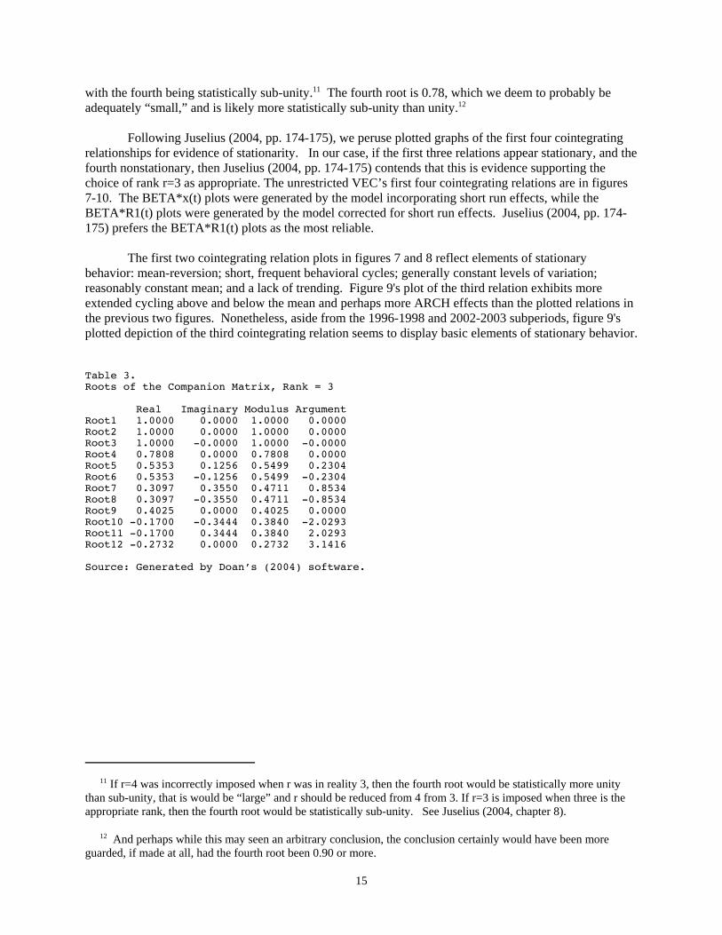
with the fourth being statistically sub-unity.11 The fourth root is 0.78, which we deem to probably beadequately “small,” and is likely more statistically sub-unity than unity.12

Following Juselius (2004, pp. 174-175), we peruse plotted graphs of the first four cointegratingrelationships for evidence of stationarity. In our case, if the first three relations appear stationary, and thefourth nonstationary, then Juselius (2004, pp. 174-175) contends that this is evidence supporting thechoice of rank r=3 as appropriate. The unrestricted VEC’s first four cointegrating relations are in figures7-10. The BETA*x(t) plots were generated by the model incorporating short run effects, while theBETA*R1(t) plots were generated by the model corrected for short run effects. Juselius (2004, pp. 174-175) prefers the BETA*R1(t) plots as the most reliable.

The first two cointegrating relation plots in figures 7 and 8 reflect elements of stationarybehavior: mean-reversion; short, frequent behavioral cycles; generally constant levels of variation;reasonably constant mean; and a lack of trending. Figure 9's plot of the third relation exhibits moreextended cycling above and below the mean and perhaps more ARCH effects than the plotted relations inthe previous two figures. Nonetheless, aside from the 1996-1998 and 2002-2003 subperiods, figure 9'splotted depiction of the third cointegrating relation seems to display basic elements of stationary behavior.

Table 3.Roots of the Companion Matrix, Rank = 3

Real Imaginary Modulus ArgumentRoot1 1.0000 0.0000 1.0000 0.0000Root2 1.0000 0.0000 1.0000 0.0000Root3 1.0000 -0.0000 1.0000 -0.0000Root4 0.7808 0.0000 0.7808 0.0000Root5 0.5353 0.1256 0.5499 0.2304Root6 0.5353 -0.1256 0.5499 -0.2304Root7 0.3097 0.3550 0.4711 0.8534Root8 0.3097 -0.3550 0.4711 -0.8534Root9 0.4025 0.0000 0.4025 0.0000Root10 -0.1700 -0.3444 0.3840 -2.0293Root11 -0.1700 0.3444 0.3840 2.0293Root12 -0.2732 0.0000 0.2732 3.1416

Source: Generated by Doan’s (2004) software.

16

Beta1'*X(t)

1992 1993 1994 1995 1996 1997 1998 1999 2000 2001 2002 2003 2004-485.0-482.5-480.0-477.5-475.0-472.5-470.0-467.5-465.0-462.5

Beta1'*R1(t)

1992 1993 1994 1995 1996 1997 1998 1999 2000 2001 2002 2003 2004-3.2-2.4

-1.6-0.8

-0.00.8

1.62.4

Figure 7Plotted cointegrating relation 1: versions with and without correction forshort run effects

Beta2'*X(t)

1992 1993 1994 1995 1996 1997 1998 1999 2000 2001 2002 2003 2004-217.5

-215.0

-212.5

-210.0

-207.5

Beta2'*R1(t)

1992 1993 1994 1995 1996 1997 1998 1999 2000 2001 2002 2003 2004-3

-2

-1

0

1

2

3


17

Figure 10 plots the fourth cointegrating relation, that displays clearer elements of nonstationarybehavioral elements than the previous three plotted relations, particularly in the panel of BETA*R1(t)plot. There are extended cycling of values in substantial parts of the sample: at the sample’s verybeginning and very end, as well as during 1995-1996 and 1999-2001. As well, the fourth relation’s plotseems heteroscedastic. Generally, figure 10 suggests that the fourth relation is non-stationary and thissuggests that perhaps the rank is 3.

As cautioned by Juselius (2004, pp. 172-176), choice should not be made with sole reliance ontrace test evidence. In summary, r=3 appears more supported than r=4 as a rank for equation 2's A whenone considers all combined evidence from the trace tests, the companion matrix’s characteristic rootswhen a rank of 3 is imposed, and an analysis of plotted behavior patterns of these first four cointegratingrelationships. We chose to impose a rank of r=3 on the error correction space.

Beta3'*X(t)

1992 1993 1994 1995 1996 1997 1998 1999 2000 2001 2002 2003 2004214

216

218

220

222

224

Beta3'*R1(t)

1992 1993 1994 1995 1996 1997 1998 1999 2000 2001 2002 2003 2004-2.7-1.8

-0.9-0.0

0.91.8

2.73.6


13 This subsample of recursive estimation, 1997:09 – 2004:09, is for the period beginning with the 1997/98 U.S.soybean marketing year and extending through the estimation period’s end. The finally restricted VEC regressorsrequired 44 degrees of freedom from 1992:12, the effective estimation period starting point with the two lagstructure. The three cointegrating relationships that emerged from the rank-restricted, adequately specified VEC areprovided as 4, 5, and 6.

18

Test for Parameter Constancy.

Figure 11 provides the recursively calculated “known beta” test of parameter constancy providedby CATS2 software and detailed in Juselius (2004, pp. 186-190). This test is typically implemented onthe adequately specified and rank-restricted (here with r=3) VEC model before the series of hypothesistests. This known beta method tests if there is constancy of estimated cointegration space estimates. This test examines if the full sample (“baseline”) model’s cointegration space coefficients could havebeen accepted as those of each model recursively estimated over the 1997:09 – 2004:09 period.13 Theplotted known-beta values in figure 11 are for two model versions: corrected and not corrected for shortrun effects (BETA_X and BETA_R1). Juselius (2004, pp. 186-190) recommends placing more relianceon the BETA_R1 plot. The known-beta values are indexed by the 95 percent critical value, and shouldideally be unity or less to indicate parameter constancy (Juselius 2004, pp. 186-190). Because most of thevalues in both the BETA_X(t) and BETA_R1 plots are unity or less, we follow Juselius (2004, pp. 186-190) and conclude that evidence at the 95 percent significance level is insufficient to reject the hypothesisof no structural change. Evidence suggests that the estimated parameters are time-invariant.

Beta4'*X(t)

1992 1993 1994 1995 1996 1997 1998 1999 2000 2001 2002 2003 2004114.0

115.2116.4

117.6118.8

120.0121.2

122.4

Beta4'*R1(t)

1992 1993 1994 1995 1996 1997 1998 1999 2000 2001 2002 2003 2004-3

-2

-1

0

1

2

3


19

Equations 4-6 are the three cointegrating relationships which emerged from imposing rank afterusing Johansen and Juselius’ (1990, 1992) well-known reduced-rank estimator. These estimates are notyet restricted for evidentially supported economic restrictions which emerge from the next section’shypothesis tests.

(4) QBEANS = -0.94*PBEANS - 1.55*QMEAL + 0.55*PMEAL + 0.05*POIL + 0.03*NAFTA + 0.15*URUGUAY + 0.09*FAIRACT + 0.10*NEWFBILL -0.03*HIDEMAND -0.15*MADCOW - 0.12*SPIKE95 = 0.002*TREND

(5) QMEAL = -0.05*PMEAL + 0.39*QBEANS + 0.03*PBEANS + 0.12*QOIL + 0.08*POIL - 0.01*NAFTA +0.08*URUGUAY + 0.06*FAIRACT + 0.003*NEWFBILL + 0.03*HIDEMAND - 0.012*MADCOW + 0.08*SPIKE95 - 0.00001*TREND

(6) PMEAL = -0.87*QMEAL - 0.01*QBEANS + 0.94*PBEANS + 0.26*QOIL - 0.55*POIL + 0.10*NAFTA + 0.02*URUGUAY + 0.01*FAIRACT - 0.04*NEWFBILL + 0.25*HIDEMAND + 0.14*MADCOW + 0.08*SPIKE95 + 0.001*TREND

Hypothesis Tests and Inference on the Economic Content of the Three Cointegrating Relations

Our procedure begins with equations 4 – 6, the three unrestricted cointegrating relations, and weconduct a series of hypothesis tests on the A = "’*$ or error-correction matrix, and then impose thoserestrictions which are statistically supported by the hypothesis test evidence (Juselius 2004, chapter 10). Johansen and Juselius (1990, pp. 194-206) and Juselius (2004, chapter 10) detail these procedures.

The test statistic is scaled by the 5% critical value

1998 1999 2000 2001 2002 2003 20040.0

0.2

0.4

0.6

0.8

1.0

1.2

1.4

1.6

1.8Be ta_X

Be ta_R1

Test of Beta(t) = "Known Beta"

Figure 11Recursively calculated “known beta” test of parameter constancy

14 The 14 variables are the six soy-based endogenous variables, seven permanent shift binary variables, and atrend.

20

Hypothesis tests on the beta coefficients take the form:

(7) $ = H*n

Above, $ is a p1 by p1 vector of coefficients on variables included in the cointegration space; H is a p1 bys design matrix, with “s” being the number of unrestricted or free beta coefficients; and n is an s by rmatrix of the unrestricted beta coefficients (Juselius 2004, pp. 245-248). Johansen and Juselius’ (1990,1992) well-known hypothesis test value or statistic is provided in equation 8.

(8) -2ln(Q) = T*j[(1-8i*)/(1- 8i)] for I = 1, 2, and 3 (=r).

The asterisked (non-asterisked) eigenvalues (8i , i = 1-3) are generated by the model estimated with(without) the tested restriction(s) imposed.

Likewise, the hypothesis tests concerning the " or adjustment speed coefficients permit acharacterization of relative speeds of error-correcting adjustment with which the system responds to agiven shock (Johansen and Juselius 1990, 1992; Juselius 2004, chapter 11). The null hypothesis or H(0)is:

(9) H(0): " = A*R

Above, A is a p by s design matrix; s is the number of unrestricted coefficients in each of the r=3 columnsof the " matrix; and R is the s by r matrix of the non-restricted or “free” adjustment speed coefficients(Juselius 2004, chapter 11). Equation 9's test statistic also applies here, and is distributed asymptoticallyas chi-squared distribution with degrees of freedom equal to the number of imposed coefficientrestrictions (Juselius 2004, pp. 206-207 and 211-213). Three sets of hypothesis tests on the betas,followed by tests on the alphas, are provided below.

Hypothesis Tests on the Betas.

There are three sets or groups of hypothesis tests on the beta coefficients. The first group of sixexamines if each endogenous variable is stationary under the imposed rank of three. Second, given thateach of the cointegrating relations has p1 or 14 variables,14 there are 14 “exclusion hypotheses” ofwhether each variable is zero in the three cointegrating relations. Given the results of these two sets oftests, a third set of sequential hypothesis tests on the individual beta estimates is provided on equations 4,5, and 6, with any statistically supported stationarity and/or exclusion restrictions imposed.

Tests of Stationarity

Juselius (2004, pp. 220-222) recommends a system-based likelihood ratio test of eachendogenous variable’s stationarity, and given the imposed rank (here r=3). She recommends such a testover univariate stationarity tests (e.g. Dickey-Fuller tests) which are independent of the cointegratedsystem’s chosen rank. Basically, the recommended likelihood ratio tests examine whether eachendogenous variable itself constitutes a separate stationary cointegrating relation, with a unity value for

15 This test can be conducted in CATS2 (beta version) in two settings: with and without inclusion of the eightdeterministic variables restricted to the cointegration space: NAFTA, URUGUAY, FAIRACT, NEWFBILL,HIDEMAND, MADCOW, SPIKE95, and TREND. We chose to include these eight deterministic variables in thetests , due to the institutional importance of events for which the variables were defined.

16 Given a rank of 3, the test values and parenthetical p-values are as follows, with the null of stationarity rejectedfor p-values less than 0.05: 11.6 (0.01) for QBEANS, 10.8 (0.01) for PBEANS, 18.1 (0.000) for QOIL, 14.5 (0.002)for POIL, 5.83 (0.12) for QMEAL, and 5.6 (0.13) for PMEAL.

17 Basically, the n matrix is the $-matrix without the beta coefficients for the variable being tested for exclusion.

18 The exclusion test values (and parenthetical p-values) for these nine variables were as follows: 50.7 (0.000) forQBEANS; 10.4 (0.02) for PBEANS; 38.2 (0.000) for QMEAL; 15.0 (0.002) for PMEAL; 12.8 (0.01) forURUGUAY; 8.9 (0.03) for HIDEMAND; 17.0 (0.001) for SPIKE95; 7.6 (0.06) for FAIRACT; and 7.5 (p= 0.06)for MADCOW. The results for the FAIRACT and MADCOW binary variables were marginal, as the test valuesreflected evidence that was insufficient to reject the null of zero-valued coefficients at the 5-percent level, but not atthe very marginal 6 percent level. Previous research uncovered evidence that the 1996 farm bill and the December2003 discovery of bovine spongiform encelopathy (BSE or “mad cow” disease) in Washington State suggested thatboth events were important in explaining the workings of these same U.S. soy-based markets (BBRS 2004, pp. 29-30; Vendatum 2004; Milling and Baking News 2004, p. 20). Given the marginal evidence of the exclusion tests forthe FAIRACT and MADCOW binary variables, as well as the cited additional evidence on the important roles that

21

the tested variable’s betas (as well as unity for the betas on the eight deterministic variables restricted tolie in the cointegration space).15 Equation 7 is rewritten as follows:

(10) $c = [b,n]

In equation 10, $c is the p1 by r (14 by 3) beta matrix with one of the variable’s levels restricted to a unitvector; b is a p1 (or 14) by 1 vector with a unity value corresponding to the relevant variable whosestationarity is being tested and for the eight deterministic components restricted to the cointegrationspace; and n is a p1 by (r-1) or 14 by 2 matrix of the remaining two unrestricted cointegrating vectors(Juselius 2004, p. 221). With nine deterministic components retained and the imposed rank of r=3, thenequation 8's test value is distributed under the null hypothesis of stationarity as a chi-squared variablewith three degrees of freedom. Evidence was sufficient to reject that four of the endogenous variableswere stationary (QBEANS, PBEANS, QOIL, and, POIL), and insufficient to reject the hypothesis thatQMEAL and PMEAL were stationary.16 Evidence thereby suggests that the modeled vector of six soy-based endogenous variables is comprised of four nonstationary or I(1) and two stationary or I(0) variablesin logged levels. In our case where r=3 and two variables are stationary: the two stationary variables eachaccounts for a separate cointegrating vector, and one cointegrating vector is a stationary combination ofindividually I(1) variables (Juselius 2004, pp. 221-222).

Tests of Beta Exclusions

The number of variables in the cointegration space of equation 2 is p1 = 14. The 14 exclusiontests examine whether each of these variables have zero coefficients in the three cointegrating relations. Failure to reject the null that a variable’s betas are zero-valued suggests that the variable should beexcluded from the cointegration space. The hypothesis test value in equation 7 would include a 14 by 3$-vector; a 14 by 13 design matrix, H, with 13 being the number of unrestricted beta coefficients in eachrelation; and a 13 by 3 matrix n of 13 unrestricted coefficients in each of the three cointegratingrelationships (Juselius 2004, chapter 10).17 Evidence at the five percent significance level was sufficientto reject the null hypothesis of zero-valued betas for the following nine variables: QBEANS, PBEANS,QMEAL, PMEAL, URUGUAY, HIDEMAND, MADCOW, FAIRACT, and SPIKE95.18 Evidence at the

the 1996 U.S. Farm Bill and BSE discovery in the Washington State have played in U.S. soy-based markets, weopted to consider total evidence as insufficient to exclude MADCOW and FAIRACT from the cointegration space.

19 The exclusion test values (and parenthetical p-values) for these nine variables were as follows: 5.3 (0.15) forQOIL, 6.0 (0.11) for POIL, 1.5 (0.69) for NAFTA, 1.6 (0.66) for NEWFBILL, and 3.7 (0.30) for TREND. In thesefive cases, evidence was soundly insufficient to reject the null hypothesis of zero-valued beta coefficients.

20 This reduced-rank estimator is summarized in Johansen (1988), Johansen and Juselius (1990, 1992), andJuselius (2004, chapters 8-10). We do not summarize this well-known reduced rank estimator here.

21 The three chosen normalizations were on QBEANS, the first cointegrating vector (CV1); on QMEAL for CV2,and on QMEAL for CV3.

22 See Babula, Bessler, Reeder, and Somwaru ‘s (2004, pp. 46-50) detailed analyses of decompositions of forecasterror variance on the same monthly U.S. system of three soy-based product markets.

22

five percent level was insufficient to reject the null hypothesis that each of the following five variableshad zero-valued beta coefficients: QOIL, POIL, NAFTA, NEWFBILL, and TREND.19 The latter fivevariables’ beta coefficients were restricted to zero.

Set of Sequential Hypothesis Tests on Individual Beta Coefficients

When the model is estimated with stationary data, one must identify the long run structure of thethree cointegrating relations which emerged as equations 4, 5, and 6 after having imposed the chosen rankof three, the five statistically supported exclusion restrictions, and the two statistically supportedstationarity conditions (on QMEAL and PMEAL). Under the rank condition of identification, oneidentifies the three relations by imposing at least r-1 or 2 restrictions on each of these cointegratingrelations (Juselius 2004, pp. 245-246).

One generally chooses testable restrictions on equations 4-6 that have been restricted for the twostationarity conditions and the five variable exclusion restrictions just discussed. These added testablehypotheses arise from theory, market knowledge, suggestions implied by coefficients generated byequations 4-6, and/or are required to meet the rank condition of identification (Juselius 2004, pp. 245-246). The test value in equation 7 is used with equation 8 (Juselius 2004, pp. 245-246). Those whichevidence fails to reject are retained, and the Johansen-Juselius reduced rank estimator20 is applied to re-estimate the three cointegrating relations with the last-accepted and statistically supported restriction(s)imposed. One repeats this process sequentially to obtain a set of finally-restricted cointegratingrelationships. Restrictions are accepted for “high” p-values above 0.05 (corresponding throughout to afive-percent level of statistical significance). Table 4 summarizes the sequential hypothesis test results.

Test set 1 (table 4) provides the first set of restrictions of the sequential hypothesis test process.[Throughout, CV1 – CV3 refer to the three cointegrating vectors or relationships.] This set identified allthree equations and included the five exclusion and two stationarity conditions supported statisticallyabove, as well as three normalizations.21 This entailed 7 restrictions on the first cointegrating relation orvector (CV1), and eight restrictions on each of the CV2 and CV3 relations. In order to meet the rankcondition of identification, we set $(QMEAL) and $(PMEAL) to zero on CV1, a relation normalized onQBEANS. We chose these two identifying restrictions because recent econometric research on these samemarkets suggested that QMEAL and PMEAL were minor contributors to QBEANS’ forecast errorvariance, and appeared logical and appropriate zero restrictions in order to identify CV1.22 The test set 1'shypothesis value was 44.8 (17 degrees of freedom or df) with a p-value of 0.000, which rejected therestrictions. We clearly must continue searching for more restrictions to add to test set 1 to generate a fullyrestricted cointegration space that is statistically supported.

23

Table 4 Sets of Sequential Hypothesis Tests on Specific Beta Estimates or Beta Estimate Subsets

Tested Restrictions, restriction numbersin each cointegrating vector (CV) Explanation/Reasons Test value, parenthetical p-value, results.

Test set 1: Testing 5 exclusion, 2 stationarity, and various identifying conditions

7 in CV1: $(QOIL) = $(POIL) =$(NAFTA)=$(TREND)=$(NEWFBILL)=0;$(QMEAL) = $(PMEAL) = 0

8 in CV2: $(QBEANS)=$(PBEANS)=$(PMEAL)=$(QOIL)=$(POIL) = 0;

$(NAFTA)=$(NEWFBILL)=$(TREND)=0

8 in CV3: $(QBEANS)=$(PBEANS)=$(QMEAL)=$(QOIL)=$((POIL)=0;

$(NAFTA)= (NEWFBILL)=$(TREND)=0

5 zero or exclusion restrictions.

2 identifying restrictions.

Needed for QMEAL stationarity.

Zero restrictions on permanent shifters fromexclusion tests.

Needed for QMEAL stationarity;

Zero restrictions from exclusion tests.

Chi-square value = 44.8 (df=17) with p-value of 0.000. As p-value is less than 0.05,reject the restrictions. More restrictioninquiry and tests needed.

Test set 2: previous test set 1’s restrictions plus: $(FAIRACT)=0 imposed on CV1 and $(POIL) =0 relaxed in CV1

7 in CV1: test set 1's 7 restrictions carriedover:plus $(FAIRACT) = 0 less $(POIL) =0

8 in CV2: test set 1's 8 restrictions retained.


Analysis, previous estimations’ results;BBRS(2004) analysis and market expertisesuggests POIL important

Chi-squared test value =44.7 (df=17) hadslight improvement (decrease) from previousestimation. But p-value of 0.003 suggestsevidence rejects rest set 2's restrictions.More restriction inquiry and tests needed.

Test set 3: previous test set 2’s restrictions less $(NEWFBILL) = 0 relaxed in all 3 CVs.

6 in CV1: test set 2's 7 restrictions retained:less $(NEWFBILL) = 0 that is relaxed.

7 in CV2: test set 2's 8 restrictions rretainedless $(NEWFBILL) = 0 that is relaxed.

7 in CV3: test set 2's 8 restrictions retained:less $(NEWFBILL) = 0 that is relaxed.

. Chi-squared test value = 53.6 (df=14)generated a p-value of 0.000 that rejectedthe restrictions. There were various non-reported improvements in CV coefficient t-values that led to our retention of test set 3'srestrictions and conclusion that we needmore restriction inquiry and tests.

Test set 4: previous test set 3's restrictions plus $(URUGUAY) = 0 in CV1.

7 in CV1: test set 3's 6 restrictions retained:plus $(URUGUAY) = 0.

7 in CV2: test set 3's 8 restrictions rretained.


Insignificant $ in CV1, previous estimation. Chi-squared value of 32.7 (df=15) improves(declines) and generates a p-value whichrejects the restrictions at the 5% level, butaccepts them at the 1% level. Morerestriction inquiry and tests needed.

Test set 5: previous test set 4's restrictions plus $(NEWFBILL)=$(MADCOW)=0 in CV1.

9 in CV1: test set 4's 7 restrictions retained:plus $(NEWFBILL)=$(MADCOW) = 0.



Insignificant $s in CV1, previous estimation Chi-squared test value improves(falls) to32.2 (df=17) and generates p-value =0.02.Evidence rejects at 5% but accepts at weaker2% level. More restriction inquiry and testsneeded.

24

Table 4Sets Sequential Hypothesis Tests on Specific Beta Estimates or Beta Estimate Subsets (continued)

Tested Restrictions, restriction numbersin each cointegrating vector (CV) Explanation/Reasons Test value, parenthetical p-value, results.

Test set 6: previous test set 5's restrictions plus $(HIDEMAND) = 0 in CV2.


8 in CV2: test set 5's 7 restrictions rretained:plus $(HIDEMAND) = 0 .


Insignificant $ in CV2, previous estimation.

Chi-square value of 34.2 (df=18) generates ap-value of 0.01 which again rejects therestrictions at the 5% level, but accepts themat the 1% level. More restriction inquiry andtests needed.

Test set 7: previous test set 6's restrictions plus $(FAIRACT) = 0 in CV3.



8 in CV3: test set 5's 7 restrictions retained:plus $(FAIRACT) = 0


Chi-square test value of 34.4 (df=19)generated a p-value of 2 percent, suggestingevidence that rejects restrictions at 5%., butaccepts them at 2%. More restrictioninquiry and tests needed.

Test set 8: previous test set 7's restrictions plus $(MADCOW) = 0 in CV3.


8 in CV2: test set 7's 8 restrictions rretained:plus $(HIDEMAND) = 0 .

9 in CV3: test set 7's 8 restrictions retained:plus $(MADCOW) = 0

Insignificant $ in CV3, previous estimation

Chi-square value of 36 (df =20) retains p-value of 0.02 from last estimation. Evidencerejects restrictions at 5% level but acceptsthem at 2% level. More restriction inquiryand tests needed.

Test set 9: previous test set 8's restrictions less two relaxations of $(TREND) …0 in CV2 and $(MADCOW)…0 in CV3.


7 in CV2: test set 8's 8 restrictions rretained:less $(TREND) = 0.

8 in CV3: test set 8's 8 restrictions retained:less $(MADCOW) = 0.

See analysis of BBRS (2004).

See analysis of BBRS (2004).

Chi-square test value of 24.3 (df=18) makesmarket improvement from last estimationand declines. The value’s p-value of 0.14soundly exceeds the 5% level and evidenceaccepts the restrictions soundly. But$(NEWFBILL) in CV2 and $(MADCOW)in CV3 are insignificant.

Test set 10: previous test set 8's restrictions plus two restrictions, $(NEWFBILL) in CV2 and $(MADCOW) in CV3 .


8 in CV2: test set 9's 7 restrictions rretained:plus $(TREND) = 0.

9 in CV3: test set 9's 8 restrictions retained:plus $(NEWFBILL) = 0.



Chi-square value of 25.7 (df=20) generatesp-value of 0.17, suggesting strong evidencein support of test set 10's restrictions that arethe finally restricted cointegrating relations.

Source: Analyses, estimations, and hypothesis test results conducted by Commission staff.

The second iteration is summarized in test set 2's restrictions: again, seven restrictions on CV1, 8on CV2, and 8 on CV3. Test set 2 differs from test set 1 in two ways: set 2 imposes the restriction$(FAIRACT)= 0 in CV1 due to an insignificant t-value when the system was estimated with test set 1'srestrictions, while $(POIL) = 0 is relaxed. Previous research suggests that POIL is important to QBEANS,CV1's left-side variable (BBRS 2004, pp. 45-49). While test set 2s’ test value of 44.7 rejects therestrictions, the p-value rose slightly from test set 1's test value. This suggests some progress towardsachieving a statistically accepted set of restrictions.

23 The newly unrestricted $[NEWFBILL] coefficients generated t-values of -2.7 and -3.9 in CV1 and CV2 thatare significant at the 5 percent level, and a t-value in CV3 of -1.7 that is significant at the 10 percent level.

25

Test set 3 relaxes the exclusion restriction that $(NEWFBILL) = 0 in all three cointegratingrelations, in addition to the already-accepted conditions in test set 2. The test value of 53.6 (df=14)generated a p-value of less than 0.05, suggesting that evidence still does not accept the restrictions andmore work needs to be done in crafting a better-defined cointegration space. However, most $[NEWFBILL] coefficients are statistically significant.23 Also, the POIL beta t-value rises markedly fromthe last estimation to 1.9. Given these beta results, we retain the restrictions and seek out more.

Test set 4 imposes $[URUGUAY] = 0 on CV1 because of a statistically insignificant t-value (-0.21) from the previous estimation with test set 3's restrictions, in addition to the restrictions of test set 3. This added zero restriction on the URUGUAY’s $ in CV1 seems to render a restriction set the sampleaccepts. The test value of 32.7 (df = 15) generated a p-value of 0.052 that accepts test set 4's restrictionsat the 5-percent significance levels. This latest estimation generated statistically insignificant coefficientson MADCOW (-1.21) and NEWFBILL (0.96) in CV1, which are set to zero, and that, with test set 4'sconditions, renders test set 5.

Test set 5 combines test set 4's restrictions with the two CV1 restrictions that were suggestedbecause of insignificant t-values during the last estimation: $(MADCOW) = $(NEWFBILL) = 0. The testvalue of 32.2 (df = 17) generated a p-value of 0.02 suggesting acceptance of the restrictions but a lowersignificance level of one-percent rather than five percent. Nonetheless, improved and strong patterns ofstatistical significance emerged for all four (non-normalized) variables remaining in CV1 as seen from thefollowing t-values: $(PBEANS), t-value = -11.4; $(POIL), t-value = -3.6; $(HIDEMAND) , t = -5.1; and$(SPIKE95), t = -4.6. All CV1 right-side coefficients are strongly significant, and effort is placed ontesting for and imposing emergent restrictions on the remaining two cointegrating relations to achieve anoverall acceptable basket of error correction space restrictions. The most obvious test that emerges fromthis estimation with test set 5's restrictions imposed is a zero restriction on $(HIDEMAND) in CV2 due tothe insignificant t-value of -0.96. This restriction is added to test set 5's restrictions to render test set 6 intable 4.

Test set 6 combines test set 5's restrictions with a new CV2 restriction that $(HIDEMAND) = 0 asjust mentioned. The 34.2 test value (df = 18) generated a p-value of 0.01, although evidence at the fivepercent level was still sufficient to reject the restrictions, implying a need for more statistical inquiry. Thesecond CV2 seems reasonable, with all coefficients having generated a significant t-value. However, $(FAIRACT) in CV3 generated a t-value of 0.42, which suggests that the restriction of the coefficientbeing zero in CV2 should be added to the restriction set. Test set 7 is test set 6 plus $(FAIRACT) = 0 inCV3, and the 34.4 test value reflects acceptance at the 2- percent, level. However, $(MADCOW)generated a t-value of -1.53 suggesting that the restriction of $(MADCOW) = 0 should be added to test set7 to form test set 8 in table 4.

Test set 8 adds $(MADCOW) = 0 in CV3 to test set 7's restrictions. The test value of 36 generateda p-value of 2 percent suggesting acceptance at a low of a significance level. However, perusal of the dataplots and results from previous research suggest that perhaps two restrictions in CV2 should be relaxed: relaxing $(TREND) = 0 as trend may be present for QMEAL, the normalized CV2 variable, and relaxing $(MADCOW) = 0 for PMEAL, CV3's normalized variable (BBRS 2004).

Test set 9 is test set 8 less two restrictions that are relaxed: $(TREND) = 0 in CV2 and $(MADCOW) = 0 in CV3. Clearly, this reduced set of restrictions enhances evidence of acceptance, withthe test value of 24.3 having generated a p-value of 0.14, far above the decision rule level of 0.05. Evidence accepts the test set 9 restrictions. However, this estimation generated two beta coefficients

24 The weak exogeneity test values and (parenthetical) p-values were as follows: 51.5 (0.000) for QBEANS; 8.8(0.03) for PBEANS, 24.7 (0.000) for QMEAL, 13.5 (0.004) for PMEAL, 15.2 (0.002) for POIL, and 6.3 (0.099) forQOIL. Evidence was sufficient at 5 percent or less to reject the null of zero-valued " coefficients for all endogenousvariables except QOIL. Evidence was sufficient at a significant level just below 10 percent to reject the nullhypothesis of QOIL’s weak exogeneity. Given the analysis of BBRS (2004), and the effects that non-soy oil has onmarket-clearing quantity of soy oil, we decided to treat QOIL as fully endogenous, although at a slightly lowerconfidence level than the other five variables. BBRS (2004) suggested that of the three markets, soy oil is the mostinfluenced by non-soy markets due to soy oil’s substitution in uses with other vegetable oils.

26

which are not significant, and whose values should perhaps be restricted to zero: $(NEWFBILL) =0 inCV2 because of a t-value of -0.46 and $(MADCOW)=0 in CV3 because of a t-value of -1.3. These twozero restrictions are added to test set 9 to render test set 10 in table 4. A test value of 25.7 (p-value of0.17) strongly accepts the test set 10 restrictions.

Hypothesis Tests on the Adjustment Speed or " Coefficients.

We conducted hypothesis tests for exogeneity of the six endogenous soy-based variables. Ineffect, such a test examines whether each variable’s " coefficients in the r=3 cointegrating relations arezero. If evidence suggests that a variable’s " coefficients are zero in the three cointegrating relations,while some of the variable’s beta coefficients are statistically nonzero, then one considers the variable asweakly exogenous (Juselius 2004, pp. 231-232). A weakly exogenous variable influences the errorcorrecting processes through non-zero beta coefficients, but does not itself adjust to the error correctionprocess (Juselius 2004, pp. 231-232). In equation 9, and given that r=3 and p=6: the "- matrix is a 6 by 3matrix of adjustment speed matrix with a row of zeros for the variable being tested for weak exogeneity; Ais a 6 by 5 design matrix (with 5 being the number of nonzero alphas in each of the three columns ofalphas); and R is a 5 by 3 matrix of nonzero alphas (see Juselius 2004, pp. 231-231). Basically, the Rmatrix is the alpha matrix without the "’s that are being tested as zero. The test value in equation 8 isdistributed as a chi-square distribution with 3 degrees of freedom (three single alpha coefficients beingzero-restricted). Evidence in all cases was sufficient to reject the null hypothesis of weak exogeneity.24

Economic Analysis of the Three Cointegrating Relationships for the U.S. Soy-Based Markets

The three fully identified and restricted cointegrating relationships are in equations 11, 12, and 13,which are followed by the adjustment speed (") coefficients. Parenthetical values below the $- and "-coefficients are t-values. Clearly these estimates display notable formidable statistical strength.

(11) QBEANS = -0.90*PBEANS + 0.16*POIL + 0.27*HIDEMAND + 0.22*SPIKE95 (-13.1) (+3.5) (+3.5) (+4.8)

(12) QMEAL = +0.10*URUGUAY + 0.05*FAIRACT - 0.07*MADCOW - 0.07*SPIKE95(+3.8) (+6.4) (-3.9) (-6.1)

(13) PMEAL = -0.20*URUGUAY - 0.24*NEWFBILL + 0.60*HIDEMAND + 0.44*SPIKE95 + 0.001*TREND (-5.3) (-3.5) (+5.4) (+5.7) (+7.0)

27

ALPHA Alpha1 Alpha2 Alpha3)QBEANS -0.7016 -0.5071 0.3476 (-8.3080) (-2.5745) (6.2544))PBEANS -0.1101 0.3565 0.0178 (-2.4944) (3.4643) (0.6140))QMEAL 0.0039 -0.4958 -0.0041 (0.1087) (-5.9777) (-0.1768))PMEAL -0.1002 0.2082 -0.0684 (-1.6554) (1.4750) (-1.7185))QOIL 0.0794 0.0603 -0.0517 (2.2770) (0.7415) (-2.2523))POIL -0.1585 0.5851 0.0870 (-2.5910) (4.1007) (2.1619)

Of the three relations, equations (12) and (13) are attributed to the stationary variables of QMEAL andPMEAL, respectively. Equation 11 is a stationary linear combination of individually nonstationaryendogenous variables, and has substantial economic interest as a demand function for soybeans. As well,the coefficients generated by the permanent shift binary variables in all three CVs provide economicallyinteresting interpretations. The $ coefficients on the endogenous variables were generated by a modelformulated in natural logarithms, and may be taken as long run elasticities of response (Johansen andJuselius 1990, 1992; Juselius 2004, chapter 5). The error-correction coefficients in equations 11 through13 reflect a set of strongly significant long run response relationships.

An Economy-Wide U.S. Demand for Soybeans.

The first cointegrating relationship appears to be a demand for soybeans. Own-price or PBEANSgenerated a negative and highly significant coefficient in equation 11. As well, having normalizedequation 11 on soybeans quantity conceptually places QBEANS in positive form above the equilibrium onthe relation’s left side, whereby the adjustment coefficient corresponding to QBEANS in the first relation(column) above is negative (-0.702), very significant (t = -8.31), and suggestive of a demand’s downwardadjustment towards long run equilibrium (following Juselius 2004, towards the “attractor set”). Thehighly significant PBEANS or own-price coefficient (t-value = -13) of -0.90 suggests a long-run own-priceelasticity of demand that approaches unity. Given that the error correction space illuminates equilibriumrelationships in the long run, presumably over two or more soybean harvests, it is not surprising that thiselasticity approaches unity. As expected, a rise in the price of soy oil would augment the demand for soybeans, with each percentage rise in POIL inducing, on average historically, a 0.16 percentage rise inQBEANS. The two periods of enhanced world oilseed demands rendered a rise in QBEANS demand, assuggested by the positive and strongly significant coefficients in equation 11 on HIDEMAND andSPIKE95.

Analysis of Deterministic Error Correction Components.

Trend appears to be unimportant, with zero-restrictions on $(TREND) statistically supported forthe first two cointegrating relationships, and with a statistically significant but very small $(TREND) valueof 0.001 supported for the third cointegrating relationship. Demand side influences seemed to dominatesupply-side influences during the 2003:09-21004:09 period for which the HIDEMAND binary variablewas defined: $(HIDEMAND) is positive and significant in both the CV1 normalized on QBEANS andCV3 normalized on PMEAL. HIDEMAND’s coefficient was a highly significant 0.25 for CV1normalized on QBEANS, and a highly significant 0.60 on CV3 normalized on PMEAL. Although BBRS(2004) cited anecdotal evidence to the contrary immediately after the December 2003 BSE discovery inWashington State, the discovery appears to have had minor effects on the soybean market. Evidencesupported MADCOW’s inclusion in only the second CV normalized on QMEAL, and while significant,

25 Note that this is the algebraic equivalent of the finally restricted cointegrated VEC obtained above, andincorporates the reduced rank restriction of r=3, all imposed restrictions on the cointegration space, and hence differsfrom the unrestricted levels VAR in equation 2 developed to achieve adequate statistical specification via theutilization of the sources of non-normal statistical information.

28

the coefficient of -0.07 is modestly valued. This value suggests that market-clearing quantities of mealmay have been diverted to feed through stock depletion, although the coefficient’s -0.07 value indicates anear-zero influence.

SPIKE95 was defined for the May 1995:05 – 1997:08 period to account for the influences of thehigher prices and demand levels for oilseeds worldwide. SPIKE95 generated a significant and positivecoefficient on PMEAL in equation 13, and a negative, significant, but modestly valued coefficient onQMEAL in equation 12. These SPIKE95 coefficients suggest dominating demand conditions for soyproducts, with increases in both QBEANS and the price of its end product (PMEAL).

Directed Graphs and Innovation Accounting Analysis

We summarize dynamic soy product relationships through an analysis of forecast error variance(FEV) decompositions. We manipulated the parameters of the estimated error correction mechanism toobtain the levels VAR equivalent of the fully-restricted cointegrated VEC model (hereafter, the VEC-equivalent levels VAR).25 We then analyzed the FEV decompositions from this VEC-equivalent levelsVAR to summarize the dynamic relations among the endogenous soy-based variables.

Incorporation of information embedded in contemporaneously correlated errors or innovations iscrucial to valid analysis of FEV decompositions (Sims, 1980; Swanson and Granger, 1997; Bessler, Yang,and Wongcharupan 2002, p. 811). Following Bessler, Yang, and Wongcharupan (2002, pp. 811-812), wefollowed a “Bernanke (1986) ordering factorization” that requires writing the innovation vector, say e(t),from the estimated error correction model as : Ae(t) = v(t),where A is a 6 by 6 matrix and v(t) is a 6 by 1vector of orthogonal shocks. It was once common in VAR-type analysis to rely on a Choleskifactorization, so that the A matrix is lower-triangular to achieve a just-identified system incontemporaneous time. We apply the TETRAD-II directed graph algorithm (described below). A directedgraph is an assignment of causal flow (or lack thereof) among a set of endogenous variables (vertices)based on observed unconditional correlation and conditional (or partial) correlations (see Bessler andAkleman 1998).

The application of directed acyclic graphs or DAGs involves the theoretical work of Pearl (1995)and the TETRAD-II algorithms in Spirtes, Glymour, and Scheines (2000). Following Bessler andAkleman (1998), we use TETRAD-II to construct a DAG on innovations from the VEC-derived levelsVAR that incorporates the statistically supported and imposed rank and hypothesis test restrictionssummarized in tables 2 and 4. The algorithm is a set of commands that begins with a set of relationshipsamong variables (innovations from each VAR equation) and proceeds step-wise to remove edges betweenvariables so as to direct causal flow in contemporaneous time (Bessler and Akleman 1998, p. 1145). Briefly, one begins with a complete, undirected graph that places an undirected edge between everyvariable in the system (every variable in set V) (Jonnala, Fuller and Bessler 2002, p. 115; Bessler, Yang,and Wongcharupan 2002, p. 811-812). Edges between variables are removed sequentially on the bases ofstatistically zero correlations or conditional correlations (Bessler, Yang and Wongcharupan 2002, p. 812;Jonnala, Fuller, and Bessler 2002, p. 113; and Bessler and Akleman 1998, p. 1145). These conditioningvariable(s) comprise the notion of a “sepset” that is, in turn, utilized to assign the direction of causal flowbetween variables that remain connected after all possible conditional correlations have been passed asnonzero (Bessler, Yang, and Woncharupan 2002, p. 812; Bessler and Alkeman 1998, pp. 1144-1146).

26 Edges are directed by considering variable triples X-Y-Z, where X and Y are adjacent, as are Y and Z, but Xand Z are not adjacent. Edges are directed for the triple as XºY»Z if Y is not in the sepset of X and Z (Bessler andAkleman 1998, p. 1145; Jonnala, Fuller, and Bessler 2002, p. 115). If XºY, Y and Z are adjacent, X and Z are notadjacent; and there is no arrow directed at Y, then one orients X–Z as YºZ. Should a directed path exist from X toY and there is an edge between X and Y, then one directs X – Y as XºY (Bessler and Akleman 1998, p. 1145).

27 We note recent research cautioning readers not to lose sight that the causal relationships implied in the directedgraph of figure DAG are for contemporaneous time, and reflect only the relationships among the six endogenousvariables at the shorter run horizons, of say six months or less (BBRS 2004, p. 39). As will be seen, a different andfar richer interplay of causality patterns among the six variables emerges when the FEV decompositions, whichreflect total causality, in contemporaneous time and over time as well, are examined. See BBRS (2004, p. 39).

29

Consider variables X, Y, and Z in a variable set V; the goal is to impose a directed edge among sets ofvariables: XºYºZ, X»Y»Z, XºY»Z, etc.26

DAGs order the six endogenous variables in contemporaneous time. The starting point is figure12, the completely unrestricted or undirected graph of all possible edges between the six variables. Asnoted in Bessler and Akleman (1998, pp. 1145-1146), there is a two stage process for using DAGs toestablish a system of contemporaneously causal orderings among the six soy-based variables. First, theTETRAD-II algorithm analyzes the unconditional correlations, eliminates the statistically zero edges, andretains the statistically nonzero ones (Scheines et. al. 1994; Spirtes, Glymour, and Scheines 2000). Andsecond, TETRAD-II performs a similar analysis on all conditional correlations, given the first stage’sretained and statistically nonzero unconditional correlations: one omits the statistically zero ones andretains the statistically nonzero ones. The edges that emerge from the two-stage TETRAD-II selectionalgorithm are then imposed on the matrix of contemporaneous innovations on the VEC-derived levelsVAR (Bessler and Akleman 1998).

There has been a series of recent DAG applications to VAR and cointegrated VEC models ofvarious agricultural markets, and these applications provide detailed explanations of the workings anddirected edge selection process of the TETRAD-II algorithm: Bessler and Akleman (1998); Bessler, Wang,and Wongcharupan(2002); Babula, Bessler, and Payne (2004), and BBRS (2002). Such detailedexplanations are therefore not provided here and readers interested in such detail are referred to thisresearch. Figure 13 provides the edges imposed on the VEC-derived levels VAR. All directed edges infigure 13 were generated from the two-stage TETRAD-II process, except for one undirected edge betweenPBEANS and PMEAL. Previous DAG work on this same database found strong evidence of a directededge of PBEANSºPMEAL (BBRS 2004, pp. 37-39). We included this latter directed edge as part offigure 13’s system of edges imposed on the VEC-derived levels VAR contemporaneous innovation matrix(Bessler and Akleman 1998).

The data strongly accept figure 13’s contemporaneous causal relationships when imposed on theinnovation matrix of the VEC-derived levels VAR. Doan (1996, p. 8.10) provides a likelihood ratiostatistic that tests the null hypothesis that the imposed DAG-suggested causal relationships in figure 13 areconsistent with or accepted by the data, and the statistic is distributed as a chi-square variable. One fails toreject the null of data acceptance for p-values above 0.05, corresponding to the 5-percent level of statisticalsignificance. Our test statistic of 3.2 (seven degrees of freedom) generated a p-value of 0.86, that farexceeds 0.05, and thereby suggests strong evidence of the data’s acceptance of the contemporaneouslycausal relationships suggested by TETRAD-II in figure 13.27

30

Source: Commission staff analysis.

Figure 13TETRAD-suggested directed acyclic graphon innovations from an error-correctionmodel on U.S. soybean complex

Source: Commission staff analysis.

Analysis of Forecast Error Variance Decompositions

QBEANS (Y1)

QMEAL (Y3)

QOIL (Y5) POIL (Y6)

PMEAL (Y4)

PBEANS (Y2)

Figure 12Undirected graph of the six soy-based variables

31

Analysis of forecast error variance (FEV) decompositions is a well-known accounting method for residuals or innovations, and is closely related to Granger causality analysis (Bessler 1984, p. 111; Sims1980, 1988). While both tools provide evidence on the existence of causal relations among two variables,analysis of FEV decompositions provides well-known extensions to Granger causality tests (BBRS 2004). A modeled endogenous variable’s FEV is attributed at alternative (here monthly) horizons to shocks ineach endogenous variable (including itself). As a result, analysis of FEV decompositions not onlyprovides evidence of the simple existence of a causal relationship among two variables, but it also illuminates the strength and dynamic timing of such a relationship (Saghaian, Hassan, and Reed 2002, p.107; Bessler 1984, p. 111). Table 5 provides the FEV decompositions for the six soy-based variables.Such decompositions reflect the causal relations embedded in both the model’s lag structure serially overtime, as well as the DAG-suggested contemporaneous causal relationships which emerged from applyingthe methodologies of Bessler and Akleman (1998).

A variable is considered exogenous (endogenous) when large (small) proportions of its FEV areattributed to its own movements (that is, to own-variation). Likewise, a variable’s endogeneity is suggestedwhen large proportions of its FEV are attributed to variation in the system’s other endogenous variables(Bessler 1984; Goodwin, McKenzie, and Djunaidi 2003, pp. 488-489). As well, decompositions of two ormore variables may be summed at a particular horizon for a “collective” effect: for example, at a chosenhorizon, the collective effect of the three soy-based prices on one of the modeled soy-based quantities canbe summed and examined. Patterns of FEV decompositions are provided in table 5.

Table 5 Decompositions of Forecast Error Variance Generated by the Levels VAR Equivalent of the Fully-Restricted Cointegrated VEC with Directed Acyclic Graphs.

Percentage of Forecast Error Variance Explained by

VariableExplained

MonthlyHorizon QBEANS PBEANS QMEAL PMEAL QOIL POIL

QBEANS 1 79.89 8.43 9.35 0.06 1.94 0.33

2 75.56 8.28 12.2 1.18 1.94 0.83

4 65.24 8.14 20.14 3.94 1.79 0.73

6 58.19 7.50 25.26 6.53 1.85 0.68

12 56.44 6.10 34.38 11.57 2.10 0.55

18 45.30 5.25 39.86 14.61 2.24 0.47

24 37.56 4.67 43.52 16.67 2.34 0.41

32

Table 5Decompositions of Forecast Error Variance Generated by the Levels VAR Equivalent of the Fully-Restricted Cointegrated VEC with Directed Acyclic Graphs (continued).


VariableExplained


PBEANS 1 0.38 98.08 0.24 0.03 0.43 0.85

2 0.76 96.28 0.48 0.10 0.66 1.72

4 1.00 94.40 0.68 0.24 0.76 2.79

6 1.13 93.74 0.69 0.31 0.75 3.29

12 1.21 93.22 0.67 0.37 0.72 3.78

18 1.25 93.07 0.65 0.39 0.72 4.93

24 1.26 93.02 0.65 0.39 0.68 4.00

QMEAL 1 1.15 2.29 94.65 0.25 1.02 0.63

2 2.63 5.28 89.95 0.30 1.72 0.57

4 5.55 8.99 81.73 0.59 2.71 0.44

6 7.09 10.70 77.91 0.78 3.17 0.35

12 9.02 12.93 73.08 1.02 3.72 0.23

18 9.81 14.00 70.95 1.10 3.94 0.19

24 10.25 14.70 69.69 1.14 4.06 0.16

PMEAL 1 0.71 67.48 0.01 30.07 1.63 0.11

2 1.11 70.16 0.60 25.37 2.69 0.07

4 1.95 71.95 1.20 21.45 3.41 0.04

6 2.35 72.56 1.50 19.89 3.66 0.04

12 2.71 73.25 1.75 18.39 3.86 0.04

QOIL 1 0.10 0.96 19.49 0.31 76.79 2.36

2 1.16 0.66 22.17 0.21 73.74 2.07

4 2.24 0.50 26.11 0.12 69.37 1.67

6 2.66 0.48 27.59 0.08 67.68 1.52

12 3.09 0.46 29.18 0.04 65.89 1.33

18 3.26 0.44 29.73 0.03 65.27 1.27

24 3.35 0.42 29.99 0.03 64.97 1.24

33

Table 5Decompositions of Forecast Error Variance Generated by the Levels VAR Equivalent of the Fully-Restricted Cointegrated VEC with Directed Acyclic Graphs (continued).


VariableExplained


POIL 1 0.21 45.22 1.64 9.22 0.12 43.58

2 0.19 40.85 1.95 10.23 0.28 46.51

4 0.11 35.46 3.13 11.03 0.63 49.63

6 0.12 32.99 4.03 11.24 0.85 50.78

12 0.13 30.53 5.10 11.32 1.08 51.87

18 0.13 29.69 5.49 11.28 1.16 52.24

24 0.13 29.27 5.74 11.21 1.21 52.43

The quantity of soybeans is noticeably exogenous at horizons of four months or less when from 65percent to 80 percent of its behavior is attributed to own-variation. Thereafter, own-variation accounts fordecreasing proportions of QBEANS’ forecast error variance or FEV, that falls to 38 percent by the 24-month horizon. Soybeans quantity appears particularly influenced by the soy meal market. Meal marketeffects on QBEANS are particularly noticeable as horizons extend to 6 months and longer – beyond theinfluences of a single annual crop. At horizons of six months or more, soy bean planting decisions in thenorthern and southern production sectors, with harvests at approximately opposing dates in a calendaryear, appear to affect the worldwide supply of soybeans. After the six month horizon, annual U.S.soybean supply or QBEANS is potentially influenced by new production (particularly from Brazil andArgentina), and the proportions of QBEANS variation collectively attributed to the soy meal marketvariables in table 5 rise from 32 percent to 60 percent by month-24. As expected, the price and quantity ofmeal crushed from QBEANS has an important influence on the quantity of soy beans.

As expected, soybean price appears highly exogenous. Among the demand and supply factors,PBEANS behavior may be particularly influenced by the available quantity of soybeans, that in turn, islargely determined by climate, especially at horizons of six months and less. PBEANS may further beexogenized by the effects of the U.S. Department of Agriculture’s (USDA’s) price support program usinga loan rate instrument.

Soy meal quantity is relatively more exogenous at short run horizons (4-6 months or less) than atthe longer horizons. From 82 percent to 95 percent of QMEAL’s variation is attributed to own-variation,and own-variation’s contributions ultimately fall to 70 percent by the 24-month horizon. At horizonsbeyond four months, the collective influence of the soybean market variables ultimately reaches 25percent. Clearly, and as expected, the market-clearing quantity and price of soybeans have an effect on thequantities of soybeans that are crushed into soy meal.

Soy meal price is highly endogenous at all reported horizons, with as little as 18 percent and nomore than 30 percent of the PMEAL variation attributed to own-variation. Soybean price heavilyinfluences soy meal price and explains from about 67 percent to 73 percent of PMEAL’s variation at allreported horizons.

28 From USDA Agricultural Marketing Service (204, p. 3) data, each 60 pound bushel of soybeans yielded 11.06pounds (18.4%) of soy oil, 45.86 pounds (76.4%) of soy meal, and 3.08 pounds (5.2%) of other materials. For morediscussion, see BBRS (2004, p. 45).

29 During 2003/2004, soybean oil accounted for 32% of the world production of 100 million metric tons or mmtof major vegetable oils, while palm oil accounted for 28%, rapeseed oil for 14%, and “other” oils for 26% (USDA,FAS 2004 a, b). World soybean oil production represented 18% of the 129 mmt of major vegetable oils, animal fats,fish oil, and butter (i.e., all fats and oils) (Oil World 2003). See also BBRS (2004, pp. 45-46).

34

Soy oil quantity is rather exogenous with from 65 percent to 77 percent of its FEV attributed toown variation. As expected with co-products, QOIL is also heavily associated with variation in its co-product, QMEAL, the variation of which explains up to 30 percent of QOIL’s FEV.

It is not surprising that POIL behavior appears collectively driven by own-variation and PBEANSmovements. Of soy oil price’s variation, from 44 percent to 52 percent is attributed to own-variation; from29 percent to 45 percent is attributed to PBEANS variation; and a more minor proportion, up to about 11percent, is explained by PMEAL movements.

Overall, the FEV decomposition patterns suggest that there is a heavy causal interaction betweenthe soybeans and soy meal markets. At horizons of six months or less comprising the window of influenceof a single crop cycle, from 25 percent to 44 percent of QBEANS variation is explained by the availablequantity of soy meal clearing the market, and QMEAL and PMEAL collectively account from 32 percentto 60 percent of QBEANS variation. So the market-clearing price and quantity of soy meal heavilyinfluences the quantity of soy beans for market.

The meal market is, in turn, heavily influenced by movements in the soybean market. Mostnoticeably, no less than 67.5 percent of PMEAL’s variation is attributed to PBEANS movements. QMEAL appears influenced by the soybean market’s movements with up to 25 percent of its FEVexplained collectively by movements in QBEANS and PBEANS. So QBEANS’ behavior is heavilyinfluenced by PMEAL and QMEAL variation, while the soybean market heavily affects the soy mealmarket, particularly through movements in PBEANS.

Causal interplay among the soy oil market and the remaining two markets is largely one-way, fromthe soybeans and soy meal markets to the soy oil market: the soy oil market has little to contribute toexplaining the table 5 FEV decompositions for the soy meal and soybean markets. That the soy oil marketaffects the soybean and soy meal markets to a lesser extent than these latter two markets influence the soyoil market is not surprising for two reasons. First, soy oil accounts for only about 18 percent and soy mealaccounts for over 76 percent of the volume of a 60-pound bushel of soybeans.28 And second, whilesoybean oil is a leading vegetable oil in the world, it accounts for less than a fifth of world production ofall “fats and oils” (combined vegetable oils, and all animal fats including tallow, fish oil, butter, andlard).29 Moreover, substitution among vegetables and most animal fats is high and prices are generallyhighly correlated (Gould, Box, Perali 1991). Such a high degree of soy oil competition for andsubstitution patterns among soy oil and other fats and oil products may partially explain the relatively largeown-variation contributions (and hence the high degrees of exogeneity of) in table 5 to the FEVdecompositions for QOIL and POIL; the high levels of own-market explanations for the soy oil marketvariables in table 5; and the relatively high levels of “detachment” of the oil market from influences on thesoy meal and soybean markets in table 5. No less than 65 percent of QOIL’s variation is self-attributed,although up to 30 percent of QOIL’s FEV is explained by QMEAL movements. Aside from own-variation, POIL’s behavior is importantly affected by soybeans price, that accounts for up to 45.2 percentof POIL’s FEV.

35

Conclusions

There has been a steadily increasing number of applications of a methodology that combines thecointegrated VAR methods of Johansen (1988), Johansen and Juselius (1990, 1992), and Juselius (2004)with analysis of directed acyclic graphs to agricultural economic issues, as cited above. For perhaps thefirst time, we have implemented such an application to a monthly system of U.S. markets for soybeans, soymeal, and soybeans.

We located monthly, 1992-2004 market year data for six U.S. soy-based variables spanning threemarkets: market clearing prices and quantities for soybeans, soy meal, and soy oil. A levels VAR andultimately a fully restricted cointegrated VEC of these six variables were specified and estimated.

Following Juselius (2004), we obtained a statistically adequate levels VAR by having harnessedthe information inherent in the data’s non-normal behavioral attributes required for valid time serieseconometric regressions (Granger and Newbold 1986, pp. 1-5). The benefits of such efforts suggested inJuselius (2005,chapters 4-6) are clearly evident on perusal of table 1: evidence strongly suggests that weachieved an adequately specified statistical model.

Evidence suggested that the six soy-based variables constituted a system of four nonstationary and2 stationary variables bound together by one stationary long run cointegrating relationship that appears tobe a U.S. demand for soybeans. There appears to be a price elasticity of U.S. soybean demand of -0.90 inthe very long run. This near-unity elasticity may be justified when one considers that the cointegrationspace parameters capture market-equilibrating relationships that extend beyond the horizon of a singlecrop cycle, and to horizons of perhaps two years or more, when fewer resources (even planted area) are asfixed as in shorter run horizons. There is also a cross-price elasticity of U.S. soybean demand with respectto soy oil price of 0.16. The 1995-1997 and the 2003-2004 periods of high world demand and price levelsof soy products appeared to positively affect demand for U.S. soybeans.

While two of the three cointegrating relationships that emerged were stationary relationships forthe price and quantity of soy meal, the coefficients on the deterministic and permanent shift binaryvariables provided empirical illumination of the importance (or unimportance) of various market andinstitutional events and policy changes. The Uruguay Round’s implementation appeared to bolster theU.S. soy meal market, likely through increased production and exports. While statistically significant,QMEAL’s near-zero coefficient on MADCOW, defined for the late-2003 discovery of mad cow disease inthe United States, failed to support BBRS’s (2004) conjectures, made shortly after the discovery, that theBSE discovery would appreciably increase the demand for QMEAL as feed ingredient. The periods ofhigh soy product demand during the 1990's and during 2003-2004 suggested demand-driven forces thatresulted in both higher soy meal prices and increased depletion in soy meal stocks, supporting previousresearch’s analysis (BBRS 2004).

Analysis of the model’s decompositions of forecast error variance (FEV) illuminate further themodeled system’s patterns of dynamic interactions. Soybeans price and quantity are clearly the dominantforces in explaining behavior in the other two soy product markets, as expected with “derivative” marketswhich are driven by the price and quantity of a commodity. There is a rich, bi-directional causal interplayamong U.S. soybean and soy meal markets. But the interplay between the soy oil market and either of theother two markets is decidedly unidirectional. While QMEAL explains QOIL behavior and PBEANSnoticeably explains POIL behavior, soy oil market’s variables (QOIL, POIL) negligibly explain behaviorin the other two markets. These results support BBRS’ (2004, pp. 47-50) findings, and their explanationthat the U.S. soy oil market’s significantly interfaces with and intensely competes in markets for otheredible oils (e.g. canola and palm oils).

36

References

Babula, R., D. Bessler, and W. Payne. “Dynamic Relationships Among U.S. Wheat-Related Markets:Applying Directed Acyclic Graphs to a Time Series Model.” Journal of Agricultural and AppliedEconomics 36, 1(April 2004):1-22.

Babula, R., D. Bessler, J. Reeder, and A. Somwaru. “Modeling U.S. Soy-Based Markets with DirectedAcyclic Graphs and Bernanke Structural VAR Methods: The Impacts of High Soy Meal and SoybeanPrices.” Journal of Food Distribution Research 35,1(Nov., 2004):29-52.

Bernanke, B. “Alternative Explanations of the Money-Income Correlation.” Carnegie-RochesterConference Series on Public Policy 25(1986):45-100.

Bessler, D. “An Analysis of Dynamic Economic Relationships: An Application to the U.S. Hog Market.”Canadian Journal of Agricultural Economics 32,1(1984):109-24.

Bessler, D. and D. Akleman. “Farm Prices, Retail Prices, and Directed Graphs: Results for Pork and Beef.” American Journal of Agricultural Economics 80, (1998):1144-49.

Bessler, D., J. Yang, and M. Wongcharupan. “Price Dynamics in the International Wheat Market:Modeling with Error Correction and Directed Acyclic Graphs.” Journal of Regional Science42(2003):793-825.

Dickey, D. and W. Fuller.1979. “Distribution of Estimates for Autoregressive Time Series with a UnitRoot.” Journal of the American Statistical Association 74:427-31.

Doan, T. RATS Users’ Manual, Version 4. Evanston, IL: Estima, 1996..

Engle, R. and C.W.J. Granger. “Cointegration and Error Correction: Representation, Estimation, andTesting.” Econometrica 55(1979):251-256.

Estima. Regression Analysis of Time Series (RATS), Version 6, Reference Manual. Evanston, IL: Estima,2004.

Fuller, W. Introduction to Statistical Time Series. New York: John Wiley & Sons, 1976.

Goodwin, H.L., Jr., A. McKenzie, and H. Djunaidi. “Which Broiler Part is the Best Part?” Journal ofAgricultural and Applied Economics 35,3(2003):483-95.

Gould, B., T. Box, and F. Perali. 1991. “Demand for Food Fats and Oils.” American Journal ofAgricultural Economics 71:212-221.

Granger, C.W.J. and P. Newbold. Forecasting Economic Time Series. New York: Academic Press, 1986.

Johansen, S. “Statistical Analysis of Cointegration Vectors.” Journal of Economic and Dynamic Control12(1988):231-253.

Johansen, S. and K. Juselius. “Maximum Likelihood and Inference on Cointegration: With Applications tothe Demand for Money.” Oxford Bulletin of Economics and Statistics 52(1990):169-210.

Johansen, S. and K. Juselius. “Testing Structural Hypotheses in Multivariate Cointegration Analysis of the

37

PPP and UIP for UK.” Journal of Econometrics 53(1992):211-44.

Jonnala, S., S. Fuller, and D. Bessler. “A GARCH Approach to Modeling Ocean Grain Freight Rates.” International Journal of Maritime Economics 4(2002):103-25.

Juselius, K. The Cointegrated VAR Approach: Methodology and Applications. Draft, forthcoming textbookon the economometrics of the cointegrated vector autoregression model. Economics Institute, Universityof Copenhagen, 2004.

Milling and Baking News. “HAS Expands Safeguards to Guard Against Transmission.” Feb. 3:20.Oil World staff. 2004. “BSE Concern in the USA.” Oil World (Jan. 2, 2004), p. 2.

Oil World staff.. Oil World (Dec. 12,, 2003) pp. 1-5.

Pearl, J. “Causal Diagrams for Empirical Research.” Biometrica 82(1995):669-710.

Saghaian, S., M. Hassan, and M. Reed. “Overshooting of Agricultural Prices in Four Asian Economies.”Journal of Agricultural and Applied Economics 34,1 (2002):95-109.

Scheines, R., P. Spirtes, C. Glymour, and C. Mee. TETRADII: Tools for Causal Modeling. Pittsburgh, PA:Carnegie Mellon University, 1994.

Sims, C. “Bayesian Skepticism on Unit Root Econometrics.” Journal of Economic Dynamics and Control12(1988):463-474.

Sims, C. “Macroeconomics and Reality.” Econometrica 48(1980):1-48.

Spirtes, P., C. Glymour, and R. Scheines. Causation, Prediction, and Search. New York: Springer-Verlag,2000.

Swanson, N. and C.W.J. Granger. “Impulse Response Functions Based on a Causal Approach to ResidualOrthogonalization in Vector Autoregressions.” Journal of the American Statistical Association92(1997):357-367.

Tiao, G., and G. Box. “Modeling Multiple Time Series: With Applications.” Journal of the AmericanStatistical Association 76(1978):802-16.

U.S. Department of Agriculture, Agricultural Marketing Service. Grain and Feed Weekly Summary andSituation 32,9(Feb. 27, 2004).

U.S. Department of Agriculture, Economic Research Service (USDA, ERS). Oil Crop Outlook, (April 9,2004a): tables 8 and 10.

U.S. Department of Agriculture, ERS. Oil Crops Situation and Outlook Yearbook, various annual issues(1993-2004b).

U.S. Department of Agriculture, Foreign Agricultural Service (USDA,FAS). Oilseeds, FOP 03-04(March,2004a): table 5.

U.S. Department of Agriculture, FAS (USDA, FAS 2004b) 2004. Oilseeds: World Markets andTrade,(March, 2004b): table 3.

38

U.S. Department of Agriculture, FAS (USDA, FAS 2004c). 2004. Oil Crops Outlook (September 13,2004c):table 10.

Vendatum, S. “Ban on Meat from Downers Grows.” The Washington Post (Jan. 27, 2004):A3.

OFFICE OF INDUSTRIES WORKING PAPER U.S. … · those of the U.S. International Trade Commission ......

Documents

Transcript of OFFICE OF INDUSTRIES WORKING PAPER U.S. … · those of the U.S. International Trade Commission ......