Off the waterfront: The long-run impact of technological ... · dependent on shipping for its...

research paper seriesGlobalisation and Labour Markets

Research Paper 2015/06

Off the waterfront:

The long-run impact of technological change on dock workers

by

Zouheir El-Sahli and Richard Upward

The AuthorsZouheir El-Sahli is a post-doctoral researcher at Lund University School of Economics and

Management, Sweden.

Richard Upward is Professor of Labour Economics in the School of Economics, University of

Nottingham and an internal research fellow of GEP

Acknowledgements

The paper has benefitted from the comments of participants at workshops at the Universities ofNottingham, Sheffield (WPEG 2014), Lund, Birmingham (ETSG 2013) and Copenhagen. Thepermission of the Office for National Statistics to use the Longitudinal Study is gratefullyacknowledged, as is the help provided by staff of the Centre for Longitudinal Study Information& User Support (CeLSIUS). CeLSIUS is supported by the ESRC Census of PopulationProgramme (award ref ES/K000365/1). The authors alone are responsible for the interpretationof the data. This work contains statistical data from ONS which is Crown Copyright. The use ofthe ONS statistical data in this work does not imply the endorsement of the ONS in relation tothe interpretation or analysis of the statistical data. This work uses research datasets which maynot exactly reproduce National Statistics aggregates. El-Sahli acknowledges funding from theStiftelsen foer fraemjande av ekonomisk forskning vid Lunds Universitet.

Off the waterfront: The long-run impact of

technological change on dock workers

by

Zouheir El-Sahli

Richard Upward

Abstract

We investigate how individual workers and local labour markets adjust over a long time period

to a discrete and plausibly exogenous technological shock, namely the introduction of

containerisation in the UK port industry. This technology, which was introduced rapidly

between the mid-1960s and the late-1970s, had dramatic consequences for specific occupations

within the port industry. Using longitudinal micro-census data we follow dock-workers over a

40 year period and examine the long-run consequences of containerisation for patterns of

employment, migration and mortality. The results show that the job guarantees protected dock-

workers' employment until their removal in 1989. A matched comparison of workers in

comparable unskilled occupations reveals that, even after job guarantees were removed, dock-

workers did not fare worse than the comparison group in terms of their labour market outcomes.

Our results suggest that job guarantees may significantly reduce the cost to workers of sudden

technological change, albeit at a significant cost to the industry.

JEL classification: J5, J63, J65, F66

Keywords: Technological change, dock-workers, layoffs, employment

Outline

1. Introduction

2. Dock employment in Great Britain

3. District-level evidence

4. Data and research design

5. Results

6. Conclusions

1 Introduction

Technological change can have dramatic and long-lasting effects on the labour market. Someindustries or occupations decline, while others expand as a result of the technological change.This restructuring causes job loss and the displacement of workers from the declining indus-tries or occupations, which can have significant and long-lasting effects on employment andearnings for the affected individuals. Studies for the US include Ruhm (1991), Jacobson et al.(1993) and more recently Couch and Placzek (2010) and Davis and von Wachter (2011). Forthe UK, to which this paper refers, Upward and Wright (2013) find long-run losses (10 yearsafter displacement) in wages and employment which amount to a permanent reduction inearnings of about 10%. As well as the financial cost, there are also long-lasting effects onother worker outcomes, such as morbidity (e.g. Black et al., 2012), mortality (e.g. Eliasonand Storrie, 2009) and family break-up (e.g. Eliason, 2012).

However, the literature on job loss does not in general consider the underlying cause of thedisplacement.1 It is therefore difficult to evaluate the adjustment cost of specific technologicaldevelopments which may simultaneously affect many firms, an entire industry or occupation.This is because such technological changes often occur relatively gradually, or because theyare difficult to isolate from other changes which are occurring at the same time, or becausethe shocks may be themselves determined by the structure of the labour market. In contrast,in this paper we focus explicitly on the labour market response to a sudden, well-defined andexogenous technological shock, namely the introduction of containerisation in UK ports.

Containerisation changed the UK port industry profoundly in the space of only a fewyears, starting in the late 1960s. The new technology was massively more capital intensive,and its introduction led to a sudden decline in the use of port labour, in particular thoseworkers who loaded and unloaded cargo, known as stevedores, dockers or longshoremen.Containerisation also brought increased economies of scale and a greater concentration ofport activity (Hall, 2009). Older ports which were unsuited to the requirements of the newtechnology (such as deep water, road and rail networks) declined while new ports expandedquickly in more suitable locations. As a large open island economy, the UK was heavilydependent on shipping for its trade. London was one of the largest ports in the world beforethe advent of the container, and suffered a particularly dramatic decline. The port districts inEast London lost some 150,000 jobs between 1966 and 1976 due to the closure of the LondonDocks, around 20% of all jobs in the area.2

Beyond the effect on the port industry itself, containerisation also affected other indus-tries which were traditionally located near ports. Hoare (1986) claims that, in 1964, 40% of

1A recent exception is the work of Autor and co-authors (For example Autor et al., 2014), which considersthe effect of increased imports from China on workers’ patterns of earnings and employment.

2Source: The London Docklands Development Corporation (http://www.lddc-history.org.uk/beforelddc/index.html).

1

http://www.lddc-history.org.uk/beforelddc/index.html

http://www.lddc-history.org.uk/beforelddc/index.html

all UK exports originated within 25 miles of their port of export, and two-thirds within 75miles.3 Containerisation and the associated development of rail and road networks meant thatwarehouses and manufacturers no longer needed to locate near ports.

Our approach in this paper is to measure the cost of the technological shock to incumbentworkers. We use micro-census data to follow dock workers in England and Wales (and var-ious comparison groups) over a 40-year period from 1971 to 2011 to measure the long-runeffect. We also consider the likely spillover effect on local labour markets, rather than justthose workers directly effected.

As noted, this paper is related to the literature on worker displacement, but rather thanmeasuring the effect of firm-specific events such as closure or layoff, it measures the impactof a more general technological shock whose effects were much more widespread. Our studybears some similarity to, and uses the same data as Fieldhouse and Hollywood (1999), whostudy the effects of the collapse of the UK mining industry during the 1980s.4 They findthat only one-third of men in mining occupations in 1981 were in employment in 1991. Incontrast, half of men in the same age group who were not in mining occupations in 1981 werein employment in 1991. Their results suggest that an industry-level collapse in employmentcan have extremely large employment effects even after 10 years.5

As well as allowing us to follow workers over a very long time period (essentially theirentire working lives), the census data also has the advantage that it tracks workers regardlessof their labour market state. Typically, administrative data which come from social securityrecords (such as that used by Jacobson et al., 1993) only contain records for those periodswhen the worker is in employment. But an important development in the UK (and US)labour markets over the last 30 years has been the large increase in the number claimingvarious disability benefits (see McVicar, 2008, for a survey of the UK evidence). In the US,Black et al. (2002) show that exogenous variation in the value of labour force participationhas a significant effect on the use of disability programmes. Our data allows us to see theextent to which the new technology caused existing workers to enter different labour marketstates such as unemployment, disability or retirement.6

Our paper is also related to the literature on the effects of deregulation and containerisa-tion on dock-workers in the United States. Talley (2002) analyzes the earnings of US uniondock-workers before and after the passage of the 1984 Shipping Act, using CPS data. The

3Hall (2009) notes that “Before containerisation, ports in the developed world were all closely related to aclearly identifiable port-city and hinterland. The huge efficiencies afforded by containers loosened these highlylocal economic ties . . . ”

4Note that this collapse was not principally caused by a technological development, but rather a combinationof political and longer-run economic factors.

5In a similar vein, Hinde (1994) studies displaced workers from another industry, shipbuilding, which expe-rienced catastrophic job loss.

6But note that both Black et al. (2002) and Black et al. (2005) concern the effect of exogenous shocks on theaggregate local labour market; whereas our focus is on the adjustment cost faced by incumbent workers.

2

results show that dock-worker earnings increased after deregulation, which is attributed tothe increase in demand for dock-workers in the period after containerisation7 and increasedcapital-labour ratios. Similarly, Hall (2009) estimates the effects of containerisation andderegulation on port worker earnings in US port cities since 1975. He also uses CPS dataand constructs difference-in-difference estimates of earnings gaps between truckers, dockersand warehousers and various control groups based on workers in non-transport occupationsbased in port and non-port cities. He finds that dockers’ pay advantage over non-transportworkers also increased during the period of containerisation and deregulation. In contrast tothese papers, we use longitudinal data which allows us to assess the impact of containerisa-tion and deregulation on existing dock workers, rather than a comparison of cross-sectionsover time.

The paper is organized as follows. In Section 2 we briefly describe the process by whichUK ports became containerized as well as the evolution of dock employment in the UK.Section 3 describes the location of English and Welsh ports and provides a district-levelcomparison of labour markets defined according to the location of ports. Our methods aredescribed in Section 4, and the main set of worker-level results is provided in Section 5.Section 6 concludes.

2 Dock Employment in Great Britain

The development of container technology is described in detail in, for example, Vigarie(1999), Levinson (2006) and El-Sahli (2012). In this section we describe the most importantdevelopments as they affected the UK, with a particular focus on the effects of containerisa-tion on port labour and employment in port areas.

Container ships first docked in the UK in 1966, when services were established for thetransatlantic trade between the US and European ports in the UK, Netherlands and WestGermany (Levinson, 2006). Containerisation required major technological changes in portfacilities, and the two largest UK ports of London and Liverpool were unsuited the new tech-nology. London docks, for example, were difficult to navigate even for smaller break-bulkships,8 and larger vessels had to unload onto smaller vessels near the mouth of the river. Fur-thermore, neither London nor Liverpool allowed easy access for onward land transportation.As a result, major investments were made in new docks at Tilbury and Southampton, whileLiverpool docks were retro-fitted to handle containers in the early 1970s.

Before containerisation, dock-work was highly paid. The average full-time docker earned

7In some ports there actually appears to have been a shortage of dock workers after deregulation.8Break-bulk shipping refers to the traditional method of transporting goods in much smaller containers such

as boxes, barrels or pallets.

3

about 30% more than the average male worker in Britain in the mid-1960s (Levinson, 2006).9

In the UK, dock-work was highly regulated by the statutory National Dock Labour Scheme(NDLS) of 1947. Under the NDLS, only registered employers were allowed to hire regis-tered dock-workers to perform dock-work. Dock-workers had high levels of unionisationand industrial disputes were common before the introduction of containers (Turnbull, 2012).The introduction of containers caused further industrial conflict: unions imposed a ban oncontainer ships at Tilbury docks in January 1968, which lasted until April 1970. The disputeresulted in the negotiation of a new Dock Labour Scheme, although there were continuing in-dustrial disputes throughout the period of containerisation. The new Dock Labour Scheme in-troduced permanent employment arrangements10 and prevented non-registered dockers fromworking in ports covered by the scheme (Turnbull et al., 1996). Voluntary severance wasalso offered with generous severance pay. In 1972, another agreement was reached whichprevented the use of compulsory redundancy. Even if the port employer went out of business,the worker would be offered dock-work with another employer if he was unwilling to acceptvoluntary severance (Turnbull and Wass, 1994).

During this period of industrial disputes, an alternative port at Felixstowe was developed(essentially by installing new equipment) which, within a few years, became the largest UKcontainer port. London docks (with the exception of Tilbury) closed from 1967 onwards,with the final closures occurring in 1983.11 The Dock Labour Scheme, and its associated fullemployment protection, was finally abolished in 1989, which led to large-scale dismissals ina short period of time. At some ports the entire registered dock labour force was dismissed,and over 7,200 dockers were declared redundant between 1989 and 1992 (Turnbull, 1992;Turnbull and Wass, 1994).

Figure 1 plots the number of dock-workers and the total number of people employed inthe port industry between 1961 and 2011. The number of dockers declines slightly from1961, but falls more quickly as containerisation takes hold from the late 1960s onwards. Thetotal number employed in the Port and inland water transport industry also falls dramatically.Between 1961 and 2001 the industry lost over 72% of its employment, while the occupationof “dock-worker” lost over 90%. The effective disappearance of dock-workers accounted for60% of the total fall in employment in the industry.

9This partly reflected a compensating differential: dock-work was difficult and dangerous, with a high acci-dent rate (Vigarie, 1999).

10Previously many dock-workers were hired on a daily basis from the pool of registered workers.11Source: Port of London Authority.

4

Port and water transport

Stevedores

0

25

50

75

100

125

150

Em

ploy

men

t 000

s

1961 1971 1981 1991 2001 2011

Figure 1. Employment (000s) in port industries and stevedore occupations 1961–2011 inGreat Britain. Source: produced by authors based on published census 10% tables (1961,1971 and 2001), New Earnings Survey (1981, 1991) and Digest of Port Statistics (1968).Industry employment for 1961-1981 is employment in “Port and inland water transport”whereas 2001 is employment in “Water transport” and is therefore not directly comparable.Industry figures are for England and Wales only. Occupation employment is employmentas “Stevedore and dock labourer” in Great Britain. Figure for 1967 stevedores is averagefor the first 37 weeks of 1967 and does not include stevedores hired by ports not coveredby the Dock Labour Scheme. The number employed in ports in 1968 does not includeinland waterways.

5

3 District-level evidence

In this section we provide evidence that the process of containerisation had long-lasting ef-fects at the level of the local labour market. We do this by comparing the labour marketperformance of districts which contained a major port in the 1960s with those that did not.An advantage of this approach is that we can use published census data which includes 1961(clearly before any containerisation had started), and which covers 10% of the population,rather than 1% as in our worker-level data.

Figure 2 illustrates the location of the major ports which were in operation in Englandand Wales in the late 1967, before the process of containerisation began in the UK.12 Alsoshown are the local authority boundaries which existed at this time in England and Wales.13

Figure 2 shows clearly the importance of the traditional ports of London and Liverpool beforecontainerisation, and also that port activity was quite widely spread at this time. Figure 3shows the geographic distribution of workers in port-related industries, aggregated from the1971 Longitudinal Study.14 As we would expect, we find concentrations of dock workers inexactly those local authorities which also contained major ports.

In Figure 4 we plot the employment and unemployment rates of port local authoritiesagainst non-port local authorities over the period 1961–2011. Panel (a) shows that in 1971the employment rate in port local authorities was slightly higher than non-port local author-ities, but experienced a steeper decline between 1971 and 1981 and did not start to recoveruntil the 1991–2001 period. The employment gap between the two groups of districts is sig-nificantly wider even in 2011 than it was in 1961. Panel (b) shows a consistent pattern for theunemployment rate, although here the port-districts already had worse performance in 1971.

Panel (c) of Figure 4 shows the precipitous decline in manufacturing employment thathas occurred in the UK over the last fifty years. This decline has been even greater for localauthorities which contained major ports in 1961. Finally, panel (d) confirms that employmentin transport-related industries was nearly twice as high in port local authorities in 1961 (andin fact increased between 1961 and 1971), but then declined. The timing of these changes isentirely consistent with the idea that the introduction of containers reduced employment bothin ports but also in the associated manufacturing industries.

The above graphs may mask very interesting variations in employment patterns acrossport locations. For instance, the London Docks completely shut down following container-isation (see Section 2). One therefore expects the London labour markets to be especiallyaffected by the technological change. The Port of Liverpool, which was second only to the

12Table A1 shows that these major ports accounted for 95% of foreign sea tonnage in 1967. Information fromports.org.uk suggests that there were an additional 80 minor commercial ports in existence.

13The organisation of local government in England and Wales changed significantly in 1974 following theLocal Government Act 1972.

14We describe this data more fully in Section 4. The Longitudinal Study is not available before 1971.

6

Workington

Whitehaven

Barrow

Preston

LiverpoolHolyhead

Tyne

Tees & Hartlepool

HullGoole

Grimsby &Immingham

King's Lynn

London &Tilbury Medway

Dover

ManchesterLiverpool

Holyhead

Tyne

Tees & Hartlepool

HullGoole

Grimsby &Immingham

Boston

King's Lynn

London &Tilbury Medway

Dover

SouthamptonShoreham

Teignmouth

Plymouth

Milford Haven

Swansea

Port TalbotBristol

Newport

Cardiff

Par & Fowey

Yarmouth

Ipswich

Harwich &Felixstowe

Figure 2. Location of the largest English and Welsh ports (measured by foreigntonnage) in 1967 (Digest of Port Statistics 1968). See Table A1 in Appendix Afor a list of major ports. The size of each circle is proportional to that port’sforeign tonnage in 1967.

Port of London before the technological change in terms of activity, faced severe disruptionsbut did re-open in the early 1970s. The port was converted into a modern container port andreopened for business in 1972.

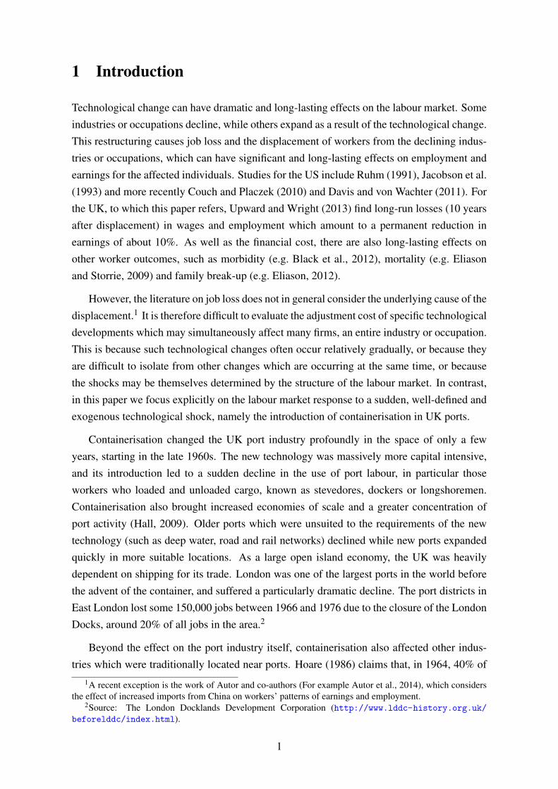
In Figure 5, we present evidence from the local London and Liverpool labour marketsand compare them with employment patterns in non-port districts. The patterns observed inFigure 4 are seen again, but are more extreme. The employment rate in London fell by nearly13 percentage points between 1961 and 1991, and went from having an employment rate farhigher than in non-port districts to having one which was lower. Liverpool’s employmentrate grew between 1961 and 1971 but then also collapsed faster than in non-port districtsbetween 1971 and 1991. These changes are mirrored in the unemployment rate, with bothLondon and Liverpool experiencing larger increases than in non-port districts. From 1971

7

>5%2-5%1-2%<1%

Figure 3. Employment in port-related industries in each Local Authority districtin 1971 (Authors’ calculations from the 1971 Longitudinal Study). Theclassification of Local Authorities which contained ports is given in Table A2 inAppendix A.

to 2011 manufacturing and transport employment fell faster in London and Liverpool thanin non port-districts, and it is striking that transport employment in London and Liverpool istoday barely higher than in non-port districts.

The evidence from local labour markets can be summarised by a district-level difference-in-difference model:

ydt = α +βDd +2011

∑s=1981

γsT s

t +2011

∑s=1981

δs(T s

t ×Dd)+ εdt , (1)

where the dependent variable is the relevant rate (employment, unemployment etc) in districtd at time t, and the treatment indicator Dd takes the value 1 if d is a district containing amajor port and 0 otherwise. The base year is 1971, rather than 1961 because it was not

8

(a) Employment rate

0.50

0.55

0.60

0.65

Em

ploy

men

t rat

e

1961 1971 1981 1991 2001 2011

Districts with no portDistricts with major port

(b) Unemployment rate

0.00

0.05

0.10

0.15

Une

mpl

oym

ent r

ate

1961 1971 1981 1991 2001 2011

(c) Manufacturing employment

0.10

0.15

0.20

0.25

0.30

0.35

0.40

Pro

port

ion

of e

mpl

oym

ent i

n m

anuf

actu

ring

1961 1971 1981 1991 2001 2011

(d) Transport employment

0.05

0.07

0.09

0.11

0.13

Pro

port

ion

of e

mpl

oym

ent i

n tr

ansp

ort i

ndus

try

1961 1971 1981 1991 2001 2011

Figure 4. Panel (a) shows proportion of population aged 16+ in employment. Panel (b) showsproportion of economically active in unemployment. Panel (c) shows proportion of employment inmanufacturing industries. Panel (d) shows proportion of employment in transport industries. Source:UK Census data. Districts containing major ports are identified in Table A2 in Appendix A. Thedefinition of “districts” changes considerably over time (section 3). “Transport industries” are notconsistently defined in the 1981 census tables and this year is excluded from panel (d).

possible to construct a consistent district-level series between 1961 and 1971 (because ofthe redrawing of district boundaries) and because published census tables from 1961 do notcover all districts. The treatment group will in this case be quite broad, and will includemany workers who were not directly employed by docks. However, as we argued in theintroduction, the containerisation of the docks had profound effects not only on dock-workers,but also on workers whose firms were located close to docks or whose firms provided servicesrelated to shipping.

The results are shown in Table 1. The estimate of β shows that the employment ratein 1971 was not significantly different in port districts relative to non-port districts, but theunemployment rate, proportion of employment in manufacturing and the proportion of em-ployment in transport were all significantly higher. The estimates of δ then show how theserates evolved over the next 40 years. Employment rates in port districts are still significantlylower (3.7pp) than those in non-port districts, even in 2011. However, the unemployment

9

(a) Employment rate

0.50

0.55

0.60

0.65

0.70

Em

ploy

men

t rat

e

1961 1971 1981 1991 2001 2011

Districts with no portLondonLiverpool

(b) Unemployment rate

0.00

0.05

0.10

0.15

0.20

Une

mpl

oym

ent r

ate

1961 1971 1981 1991 2001 2011


(c) Manufacturing employment

0.00

0.05

0.10

0.15

0.20

0.25

0.30

0.35

0.40

Pop

ortio

n of

em

ploy

men

t in

man

ufac

turin

g

1961 1971 1981 1991 2001 2011


(d) Transport employment

0.00

0.02

0.04

0.06

0.08

0.10

0.12

Pop

ortio

n of

em

ploy

men

t in

tran

spor

t

1961 1971 1981 1991 2001 2011


Figure 5. See notes for previous figure. “London” and “Liverpool” refers to those local authoritydistricts within London and Liverpool which contained major ports in the 1960s; see Table A2 inAppendix A.

effect seems to have been less permanent. Presumably this reflects the fact that those workerswho lost their jobs as a result of containerisation and the exodus of manufacturing jobs even-tually retired or left the area. In the third and fourth column we see that, relative to non-portdistricts, manufacturing and transport employment is still significantly lower than it was in1971.

The district-level results from this section suggest that labour markets which contained amajor port in the 1960s fared worse than labour markets which did not contain a major port,and that this difference has persisted for many years. Furthermore, the graphical evidencesuggests that this difference coincided with the introduction of containerisation in UK ports.This is at least suggestive of the idea that (a) the effects of containerisation were felt moregenerally than simply within the docks and (b) these effects were very long-lasting.

However, this evidence does not control for the characteristics of the workers or the in-dustries in each district. It seems plausible, for example, that districts which contained portshad different occupational and industrial structures and that these districts might have faredworse than other districts regardless of the introduction of containerisation. In addition, the

10

Emp.rate

Unemp.rate

Manuf.rate

Trans.rate

β 0.006 0.015∗∗∗ 0.032∗∗ 0.053∗∗∗

(0.006) (0.002) (0.013) (0.006)

δ 1981 −0.018∗∗∗ 0.009∗∗∗ −0.042∗∗∗

(0.004) (0.004) (0.008)δ 1991 −0.039∗∗∗ 0.018∗∗∗ −0.061∗∗∗ −0.033∗∗∗

(0.006) (0.004) (0.010) (0.005)δ 2001 −0.047∗∗∗ 0.004 −0.054∗∗∗ −0.041∗∗∗

(0.008) (0.003) (0.010) (0.006)δ 2011 −0.037∗∗∗ 0.003 −0.047∗∗∗ −0.045∗∗∗

(0.007) (0.003) (0.012) (0.006)

Number of obs. 6,830 6,830 6,830 5,464Number of districts 1,366 1,366 1,366 1,366R2 0.311 0.389 0.418 0.194

Table 1. District level difference-in-difference estimates (1971–2011). Tablereports estimates of Equation (1). “Transport industries” are not consistentlydefined in the 1981 census tables and this year is excluded from the final column.

district-level evidence does not tell us directly about adjustment costs. If, for example, work-ers move from declining districts (such as those containing ports) to expanding districts, thenadjustment costs may be low even though there are large differences in employment growthbetween districts. In the next section therefore we turn to individual level data which allow usto track incumbent workers, and which allow us to control for the pre-existing characteristicsof workers, including occupation and industry.

4 Data and Research Design

Individual micro-level data for England and Wales is taken from the Office for National Statis-tics Longitudinal Study (LS).15 The sample comprises individuals born on one of four se-lected dates during the year, and therefore represents slightly more than 1% of the populationof England and Wales. Records are linked across each 10-year census from 1971 to 2011. Aweakness of our data is therefore that we first observe workers a few years after the process ofcontainerisation started. Nevertheless, Figure 1 suggests that about two-thirds of stevedoresremained by 1971. The data include information on occupation, economic activity, housing,ethnicity, age, sex, marital status and education as well as geographic data. As well as censusrecords, the LS also contain information on events including death and migrations.

The data allows us to follow a sample of employed men in 1971 and trace patterns ofemployment or re-employment (in new occupations, industries and places of work), unem-

15This information on the LS is taken from http://celsius.lshtm.ac.uk/what.html.

11

http://celsius.lshtm.ac.uk/what.html

ployment or inactivity. Because we can do this over a long time period we can capture, formost workers, their entire working lives. We focus on groups of workers who were likelyto have been affected by the introduction of containers. These groups include dock-workers,workers in port industries and workers who work close to docks. We compare these groupsto observationally similar workers who are less directly affected by the process of container-isation.

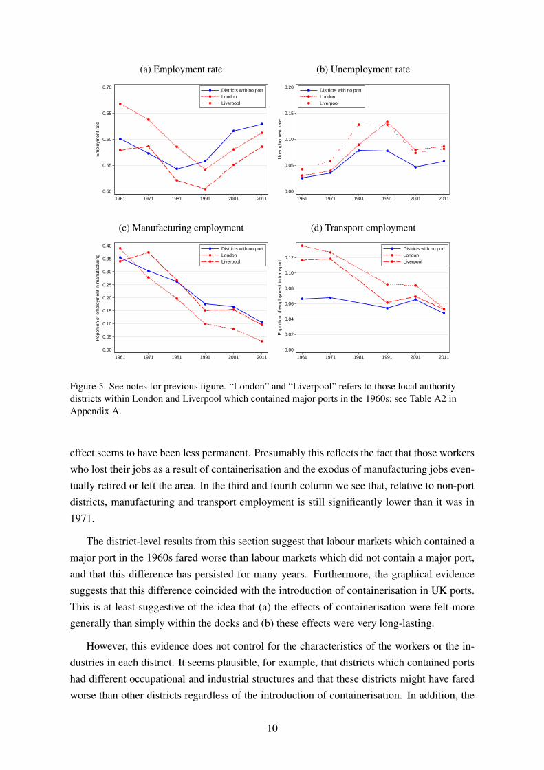
Our complete sample comprises 201,091 individuals who were employed at the time ofthe census in April 1971 as employees, apprentices, foremen and managers.16 From thesewe select only men, since all the individuals identified as stevedores in 1971 were men. Thisleaves us with 124,335 male workers observed in 1971. The first row of Table 2 shows that83% of these workers are also observed 10 years later in the 1981 census. About half of thosewho are not observed in subsequent censuses have died; the remainder could not be tracedby ONS. The attrition rate increases over each 10-year interval because the sample ages andtherefore the proportion dying increases. The remaining rows of Table 2 summarises ourmain treatment and control groups.

The first treatment group D1 is defined by occupation. The UK classification of occu-pations in use at the time of the 1971 census (Office for Population Censuses and Surveys,1970) has a specific category for “Stevedores and dock labourers.” We find 397 individualsin this occupational group, which is very consistent with the estimated number of stevedoresfrom the published census tables (see Figure 1). Rather than using all workers who are notstevedores as a control group, we restrict the control group to include only those workersin social classes 3 (“skilled manual”) and 5 (“unskilled”), since all stevedores fall into theseclasses. We also restrict the control group to exclude workers in transport industries to avoidthe potential problem that containerisation had effects on other industries in the transportsector.

The second treatment group D2 is defined by industry. The UK classification of industriesat the time of the 1971 census (Central Statistical Office, 1970) has a classification for “Portand inland water transport”. We find 759 men in this industry, which again is consistent withthe estimates from published census tables shown in Figure 1. As for D1, we also restrict thecontrol group to exclude workers in transport industries.

The third treatment group D3 is defined by geography. Using the districts defined inSection 3 (i.e. those that contained major ports in 1971), a worker is in treatment groupD3 if their place of work falls in one of those districts in 1971, and is in the control groupotherwise. To make the distinction between the geographically defined treatment and controlgroups more clear-cut, we also define two alternative control groups. In D3a we include inthe control group only workers whose place of work is in Counties (larger geographic areas)

16ONS estimates from survey data that total employment in Spring 1971 was 24.5m, suggesting that oursample is slightly less than 1% (Lindsay and Doyle, 2003).

12

1971

1981

1991

2001

2011

Ori

gina

lsam

ple,

excl

udin

gse

lf-e

mpl

oyed

and

thos

eab

ove

65in

1971

124,

335

102,

860

86,5

8566

,876

49,4

50

D1=

1A

llst

eved

ores

in19

7139

734

427

219

112

3D

1=

0A

llno

n-st

eved

ores

inun

skill

edan

dsk

illed

man

ualo

ccup

atio

nsin

1971

51,7

0642

,707

35,7

0927

,356

20,2

06

D2=

1A

llw

orke

rsin

port

indu

stry

in19

7175

963

950

136

123

4D

2=

0A

llw

orke

rsno

tin

the

tran

spor

tind

ustr

yin

1971

112,

930

93,3

7578

,652

60,9

6745

,268

D3=

1A

llw

orke

rsin

dist

rict

sw

itha

maj

orpo

rtin

1971

23,1

3419

,098

16,0

5512

,364

9,15

3D

3=

0A

llw

orke

rsin

dist

rict

sw

ithno

maj

orpo

rtin

1971

(exc

lude

sw

orke

rsin

tran

spor

tind

ustr

y)93

,153

77,0

8264

,933

50,3

5737

,360

D3a

=1

All

wor

kers

indi

stri

cts

with

am

ajor

port

in19

7123

,134

19,0

9816

,055

12,3

649,

153

D3a

=0

All

wor

kers

inco

untie

sw

ithno

maj

orpo

rtin

1971

(exc

lude

sw

orke

rsin

tran

spor

tind

ustr

y)35

,821

29,8

6025

,298

19,7

3214

,723

D3b

=1

All

wor

kers

indi

stri

cts

with

am

ajor

port

in19

7123

,134

19,0

9816

,055

12,3

6491

53D

3b=

0A

llw

orke

rsin

dist

rict

sm

ore

than

20km

from

any

port

(exc

lude

sw

orke

rsin

tran

spor

tind

ustr

y)56

,560

46,9

8039

,674

30,7

8923

005

Tabl

e2.

Defi

nitio

nof

cont

rola

ndtr

eatm

entg

roup

s.T

hesa

mpl

ein

clud

eson

lym

en;a

llof

the

wor

kers

iden

tified

asst

eved

ores

in19

71w

ere

men

.

13

which do not contain any major ports. Thus for example all workers in London are excludedfrom this control group. In D3b we include in the control group only workers whose place ofwork is at least 20km from any port.17

Once we have defined the treatment and control groups, we require information on thosesame workers in each of the following censuses up to 2011. We create a panel with five obser-vations for each individual (t = 1971,1981,1991,2001,2011). Define yit to be the outcomeof individual i at time t. These outcomes will be indicator variables capturing employmentstatus, occupational mobility, geographic mobility and mortality. Define Di to be an indicatorvariable which takes the value 1 if individual i is in the treatment group in 1971 and 0 other-wise. Define T 81

it to be an indicator variable which takes the value 1 if observation i refers toyear 1981. T 91

it , T 01it and T 11

it are defined analogously.

We measure the effect of containerisation by comparing the evolution of yit between in-dividuals in the treatment group and those in the control group. In each case the base year(1971) is such that everyone in the sample has yit = 1 because everyone in the sample isin employment (or in the census) in that year, or because their mobility status is undefined.Therefore we estimate a simplified difference model (rather than a difference-in-differencemodel as before):

yit = α +2011

∑s=1991

γsT s

t +2011

∑s=1981

δs(T s

t ×Di)+ εit . (2)

The coefficients γs capture the evolution of yit over the next three decades for individuals inthe control group, while the δ s coefficients capture the difference in the evolution of yit forthe treatment group.

We also need to consider pre-existing observed differences between the treatment andcontrol groups in 1971. For example, the treatment and control group may differ in terms ofage, education, occupation and so on. To illustrate the differences between the treatment andcontrol groups in terms of their characteristics, Table 3 compares the mean values for eachtreatment/control comparison.

For definitions D1 and D2, the treatment group is significantly older, more likely to bemarried and more likely to have educational qualifications below A-level.18 For definitionD3 (based on geography) the treatment and control groups the pre-existing differences inpersonal characteristics are much smaller. By definition, the industry and occupation of thetreatment and control groups differ for definitions D1 and D2. 91% of the D1 treatmentgroup report that they work in the transport industry. Note that we exclude from the D1 andD2 control groups those working in transport, to avoid possible spillover effects. 77% of the

17Distances are computed between the midpoint of each Local Authority using geodetic distances (Picard,2010).

18Unfortunately the census educational classification from 1971 does not distinguish between any educationalqualifications below A-level, which covers the great majority of the sample.

14

D1(stevedores vs.

other occupations)

D2(port industry vs.other industries)

D3(port district vs.other districts)

D1 = 1 D1 = 0 p-value D2 = 1 D2 = 0 p-value D3 = 1 D3 = 0 p-value

Age 42.89 38.84 [0.000] 43.54 39.10 [0.000] 39.39 39.22 [0.091]Marital status (1=single) 0.10 0.24 [0.000] 0.12 0.24 [0.000] 0.23 0.23 [0.382]Higher degree 0.00 0.00 [0.831] 0.00 0.01 [0.105] 0.01 0.01 [0.014]Other Degree 0.00 0.00 [0.635] 0.01 0.05 [0.000] 0.05 0.05 [0.086]Other qualif. above A-level 0.00 0.01 [0.145] 0.01 0.04 [0.000] 0.04 0.04 [0.674]A-level 0.01 0.03 [0.011] 0.03 0.07 [0.000] 0.07 0.06 [0.098]Below A-level 0.99 0.96 [0.006] 0.95 0.83 [0.000] 0.84 0.84 [0.018]

Primary industry 0.00 0.06 [0.000] 0.00 0.05 [0.000] 0.01 0.06 [0.000]Manufacturing 0.06 0.58 [0.000] 0.00 0.48 [0.000] 0.40 0.45 [0.000]Construction 0.00 0.14 [0.000] 0.00 0.09 [0.000] 0.08 0.08 [0.315]Energy 0.00 0.03 [0.002] 0.00 0.03 [0.000] 0.03 0.02 [0.000]Transport 0.91 0.00 1.00 0.00 0.15 0.08 [0.000]Services 0.03 0.19 [0.000] 0.00 0.35 [0.000] 0.34 0.31 [0.000]

Professional 0.00 0.00 0.01 0.05 [0.000] 0.05 0.05 [0.036]Intermediate 0.00 0.00 0.08 0.17 [0.000] 0.17 0.16 [0.006]Skilled non-manual 0.00 0.00 0.12 0.12 [0.959] 0.15 0.11 [0.000]Skilled manual 0.23 0.84 [0.000] 0.28 0.38 [0.000] 0.36 0.40 [0.000]Partly skilled 0.00 0.00 0.14 0.18 [0.001] 0.17 0.19 [0.000]Unskilled 0.77 0.16 [0.000] 0.37 0.07 [0.000] 0.09 0.07 [0.000]Other occupation 0.00 0.00 0.00 0.02 [0.000] 0.01 0.02 [0.000]

North 0.05 0.08 [0.016] 0.04 0.07 [0.011] 0.09 0.06 [0.000]Yorkshire and Humberside 0.11 0.12 [0.846] 0.10 0.10 [0.759] 0.05 0.11 [0.000]North West 0.20 0.14 [0.001] 0.25 0.14 [0.000] 0.28 0.10 [0.000]East Midlands 0.01 0.08 [0.000] 0.01 0.07 [0.000] 0.00 0.09 [0.000]West Midlands 0.00 0.13 [0.000] 0.00 0.12 [0.000] 0.00 0.14 [0.000]East Anglia 0.02 0.03 [0.136] 0.02 0.03 [0.131] 0.03 0.03 [0.063]South East 0.49 0.29 [0.000] 0.44 0.35 [0.000] 0.37 0.35 [0.000]South West 0.06 0.06 [0.487] 0.06 0.07 [0.373] 0.09 0.07 [0.000]Wales 0.07 0.06 [0.466] 0.08 0.05 [0.001] 0.09 0.04 [0.000]

Male unemployment rate (ward) 6.10 4.19 [0.000] 5.59 3.89 [0.000] 4.83 3.70 [0.000]% unskilled workers (ward) 14.49 8.32 [0.000] 12.38 7.45 [0.000] 9.51 7.07 [0.000]% semi-skilled workers (ward) 19.59 17.53 [0.000] 18.65 16.73 [0.000] 16.92 16.70 [0.000]

Number of observations 397 51,706 759 112,930 23,134 101,201

Table 3. Pre-existing differences in sample characteristics in 1971.

D1 treatment group are classified as being in social class 5 (“unskilled”) and 23% in socialclass 3 (“skilled manual”). We therefore restrict the D1 control group to the same socialclasses, but note that their distribution across those two classes is completely different. 69%of the D1 treatment group have their workplace in the South East and the North West (seeFigure 2). We also note that for all three classification D1, D2 and D3, the local labour marketunemployment rate and the proportion of unskilled employment in 1971 are significantlyhigher for the treatment groups than the control groups.

We use two methods to control for these pre-existing differences. First, we include thefull set of covariates described in Table 3 in Equation (2). Second, we explicitly “match”treatment observations with observationally similar control observations using the propensityscore method proposed by Rosenbaum and Rubin (1983). The propensity score p(x) is de-fined as the probability of being in the treatment group given a set of pre-existing observable

15

characteristics, x:p(x) = Pr{Di = 1 | xi}.

The scores are estimated from a logit model. The matching method has the advantagethat it imposes a common support on the treated and untreated observations. That is, weonly include in the control group those observations whose characteristics are such that theyhave a propensity score similar to some observations in the treatment group. In practice, thismeans we compare dock-workers, those who work in port industries, or those who work inport districts to workers who were observably similar in 1971. Because we typically have avery large control group we choose the 100 nearest matches to each treated observation butrestrict matches to be within 0.001 of the propensity for treated observations.

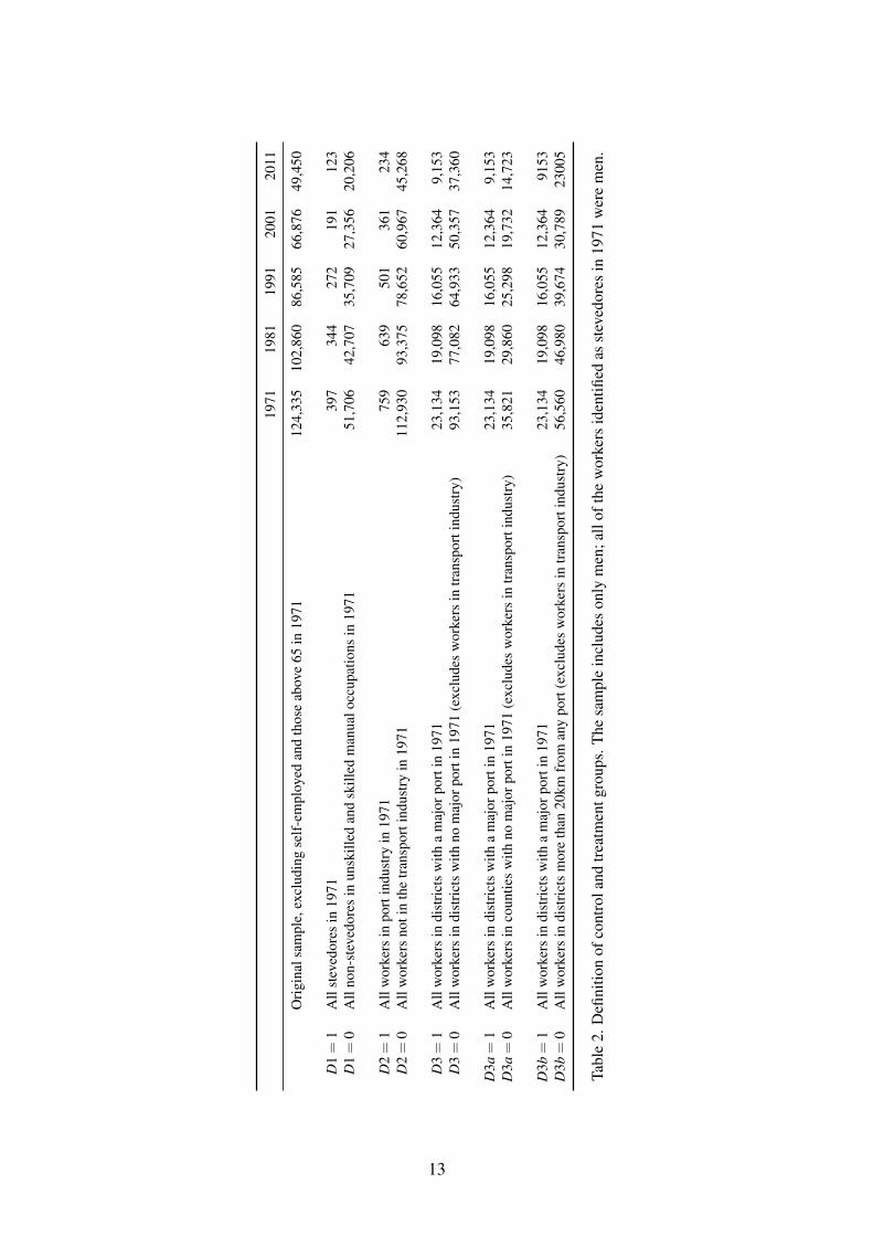
In Table 4 we report the means of the treatment and control groups after matching. In con-trast to Table 3, the observable characteristics of the treated and control samples are almost allinsignificantly different from each other. For sample D1 we match within occupation, whichis why the sample is perfectly balanced across skilled manual (25%) and unskilled (75%).Note that for D1 we do not match on industry because the treatment group consists almostentirely of workers in the transport sector, while the control group excludes the transport sec-tor. Similarly for sample D2 we do not match on sector because the treatment and controlgroups are defined by sector. Almost all the treatment observations in Table 3 are also in thematched samples shown in Table 4, which shows that almost all treated observations haveone or more observations from the control group with similar characteristics. Thus, the effectof matching is to select from the full control group a subset of observations which are moresimilar to the treatment group. For example, the matched control group D1 = 0 comprises11,886 observations drawn from the original control group of 51,706.

After matching, the effect of containerisation is estimated as the average treatment effecton the treated; see Eqn (25.40) in Cameron and Trivedi (2005) for example. In practice, this isachieved by estimating Equation (2) on the matched treatment and control groups where theobservations in the control group are weighted by the weights obtained from the propensityscore matching.

16

D1(stevedores vs.

other occupations)



D1 = 1 D1 = 0 p-value D2 = 1 D2 = 0 p-value D3 = 1 D3 = 0 p-value

Age 43.02 43.01 [0.974] 43.64 43.69 [0.945] 39.19 39.20 [0.932]Marital status (1=single) 0.09 0.09 [0.275] 0.12 0.13 [0.727] 0.23 0.23 [0.206]Higher degree 0.00 0.00 0.001 0.001 [0.989] 0.01 0.01 [0.743]Other Degree 0.00 0.00 0.02 0.02 [0.581] 0.05 0.06 [0.315]Other qualif. above A-level 0.00 0.00 0.01 0.01 [0.646] 0.04 0.05 [0.317]A-level 0.01 0.01 [0.599] 0.03 0.03 [0.872] 0.07 0.07 [0.491]Below A-level 0.99 0.99 [0.599] 0.95 0.94 [0.530] 0.82 0.82 [0.093]

Primary industry 0.01 0.01 [0.791]Manufacturing 0.47 0.47 [0.480]Construction 0.10 0.09 [0.544]Energy 0.03 0.03 [0.360]Transport 0.00 0.00Services 0.39 0.40 [0.484]

Professional 0.00 0.00 0.01 0.02 [0.767] 0.06 0.06 [0.293]Intermediate 0.00 0.00 0.08 0.08 [0.843] 0.18 0.18 [0.106]Skilled non-manual 0.00 0.00 0.12 0.12 [0.698] 0.15 0.16 [0.175]Skilled manual 0.25 0.25 [1.000] 0.29 0.28 [0.805] 0.36 0.35 [0.134]Partly skilled 0.00 0.00 0.14 0.14 [0.859] 0.16 0.16 [0.234]Unskilled 0.75 0.75 [1.000] 0.36 0.37 [0.678] 0.08 0.08 [0.746]Other Occupation 0.00 0.00 0.00 0.00 [0.805] 0.01 0.01 [0.253]

North 0.05 0.05 [0.863] 0.04 0.04 [0.780] 0.09 0.10 [0.001]Yorkshire and Humberside 0.11 0.12 [0.514] 0.10 0.09 [0.780] 0.05 0.04 [0.000]North West 0.18 0.19 [0.078] 0.24 0.25 [0.765] 0.28 0.27 [0.180]East Midlands 0.01 0.01 [0.863] 0.01 0.01 [0.641] 0.00 0.00 [0.942]West Midlands 0.00 0.00 [0.054] 0.00 0.01 [0.236] 0.00 0.00 [0.013]East Anglia 0.02 0.02 [0.787] 0.02 0.02 [0.958] 0.03 0.03 [0.689]South East 0.49 0.48 [0.263] 0.44 0.43 [0.626] 0.36 0.36 [0.538]South West 0.06 0.06 [0.466] 0.07 0.07 [0.884] 0.09 0.10 [0.023]Wales 0.07 0.07 [0.454] 0.08 0.08 [0.888] 0.09 0.09 [0.623]

Male unemployment rate (ward) 5.72 5.89 [0.010] 5.40 5.56 [0.451] 4.71 4.61 [0.003]% of unskilled workers (ward) 13.47 13.42 [0.706] 11.91 12.05 [0.736] 9.20 9.09 [0.066]% of semi-skilled workers (ward) 19.45 19.77 [0.002] 18.63 18.54 [0.275] 16.75 16.52 [0.000]

Number of observations 361 11,886 720 35,983 19,053 75,582

Table 4. Pre-existing differences in sample characteristics in 1971, after propensity score matching.Sample D1 are matched within occupations. Industry is not used for matching sample D1 because thetreatment group consists almost entirely of those working in the transport sector and the controlgroup excludes the transport sector.

17

5 Results

In this section, we present the results from estimating Equation (2) using the treatment andcontrol group definitions given in Table 2. We estimate a number of models to examinethe extent to which the treatment group experienced differential rates of: (1) attrition andmortality, (2) labour market states, (3) geographic and occupational mobility.

5.1 Attrition and mortality

We start by considering the extent to which the treatment and control groups differ in termsof their appearance in the LS. As shown in Table 2, the proportion of individuals who canbe linked across 10-year intervals declines from 83% in 1971-1981 to 74% in 2001–2011.Model (1) “In census” therefore examines whether the treatment group are more likely toexit the sample. Of the exits from the sample, around half are not linked because of deathof the respondent. The LS records year of death, from which we create an indicator variablewhich takes the value 1 if the respondent has died before the following census date. Model (2)“Died” therefore examines whether the treatment group are more likely to die.19 Estimates ofModels (1) “In census” and (2) “Died” are shown in Table 5. We estimate each model usingtreatment and control groups D1, D2 and D3 as defined in Table 2. The top panel shows theraw differences between the treatment and control groups, while the bottom panel shows thedifferences after matching on observable characteristics.20

In panel (a) of Table 5 estimates of α and γ are very similar for samples D1, D2 and D3because the (very large) control groups are similar in all three samples. Estimates of α showsthat 83% of the control group remain in the sample in 1981, while the estimates of γs showthat a further 13.5% of the control group leave the sample by 1991, 29.7% by 2001 and so on.The estimates of δ for samples D1 and D2 show that the treatment group had higher attritionrates in 2001 and 2011. In other words, workers who were stevedores in 1971 or who workedin port industries in 1971 are less likely to be observed in the sample in 2001 and 2011.However, for sample D3 the differences between the treatment and control groups are muchsmaller and generally insignificantly different from zero. Estimates of Model (2) show thatthis difference in attrition rates between the treatment and control groups is entirely due todifferent death rates. For example, the D1 treatment group are 8.1pp less likely to appear inthe sample in 2011 than the control group (δ 2011 = −0.081 with a standard error of 0.023),and this is entirely explained by the fact that they are 9.8pp more likely to have died by 2011(δ 2011 = 0.098 with a standard error of 0.025).

19Note that if an individual attrits without a recorded year of death then mortality is missing, so the mortalityoutcome is conditional on appearance in the LS up until the previous census.

20For reasons of space, OLS estimates are reported in Appendix C.

18

D1(stevedores vs.

other occupations)



Model (1)In census

Model (2)Died

Model (1)In census

Model (2)Died

Model (1)In census

Model (2)Died

(a) Raw differences

α 0.826∗∗∗ 0.081∗∗∗ 0.827∗∗∗ 0.079∗∗∗ 0.827∗∗∗ 0.079∗∗∗

(0.002) (0.001) (0.001) (0.001) (0.001) (0.001)γ1991 −0.135∗∗∗ 0.143∗∗∗ −0.130∗∗∗ 0.137∗∗∗ −0.130∗∗∗ 0.137∗∗∗

(0.002) (0.002) (0.001) (0.001) (0.001) (0.001)γ2001 −0.297∗∗∗ 0.316∗∗∗ −0.287∗∗∗ 0.306∗∗∗ −0.287∗∗∗ 0.306∗∗∗

(0.002) (0.002) (0.002) (0.001) (0.002) (0.002)γ2011 −0.435∗∗∗ 0.478∗∗∗ −0.426∗∗∗ 0.467∗∗∗ −0.426∗∗∗ 0.467∗∗∗

(0.002) (0.002) (0.002) (0.002) (0.002) (0.002)δ 1981 0.041∗∗ −0.012 0.015 0.022∗∗ −0.002 0.002

(0.017) (0.013) (0.013) (0.011) (0.003) (0.002)δ 1991 −0.005 0.020 −0.036∗∗ 0.064∗∗∗ −0.003 0.005

(0.023) (0.022) (0.017) (0.017) (0.003) (0.003)δ 2001 −0.048∗ 0.051∗∗ −0.064∗∗∗ 0.089∗∗∗ −0.006∗ 0.007∗

(0.025) (0.026) (0.018) (0.019) (0.004) (0.004)δ 2011 −0.081∗∗∗ 0.098∗∗∗ −0.093∗∗∗ 0.119∗∗∗ −0.005 0.008∗∗

(0.023) (0.025) (0.017) (0.018) (0.004) (0.004)

Number of obs. 208,412 193,905 454,756 421,673 465,148 431,429Number of ind. 52,103 49,965 113,689 108,810 116,287 111,322R2 0.114 0.150 0.109 0.146 0.109 0.146

(b) Matched on 1971 characteristics

α 0.766∗∗∗ 0.099∗∗∗ 0.786∗∗∗ 0.104∗∗∗ 0.826∗∗∗ 0.079∗∗∗

(0.008) (0.005) (0.004) (0.003) (0.002) (0.001)γ1991 −0.160∗∗∗ 0.179∗∗∗ −0.169∗∗∗ 0.188∗∗∗ −0.130∗∗∗ 0.137∗∗∗

(0.009) (0.008) (0.006) (0.006) (0.002) (0.002)γ2001 −0.363∗∗∗ 0.412∗∗∗ −0.363∗∗∗ 0.407∗∗∗ −0.290∗∗∗ 0.310∗∗∗

(0.011) (0.011) (0.006) (0.006) (0.003) (0.002)γ2011 −0.507∗∗∗ 0.597∗∗∗ −0.510∗∗∗ 0.584∗∗∗ −0.432∗∗∗ 0.474∗∗∗

(0.010) (0.010) (0.006) (0.005) (0.003) (0.003)δ 1981 0.107∗∗∗ −0.026∗ 0.056∗∗∗ 0.001 0.001 0.001

(0.019) (0.015) (0.014) (0.012) (0.003) (0.002)δ 1991 0.081∗∗∗ −0.029 0.045∗∗ −0.011 0.000 0.003

(0.026) (0.025) (0.018) (0.018) (0.004) (0.004)δ 2001 0.065∗∗ −0.045 0.050∗∗ −0.031 0.003 −0.002

(0.028) (0.029) (0.019) (0.020) (0.004) (0.004)δ 2011 0.043∗ −0.029 0.031∗ −0.020 0.007 −0.005

(0.025) (0.028) (0.018) (0.019) (0.004) (0.005)


Table 5. Differences in attrition rates and mortality between treated and control groups, 1981–2011.

19

The raw differences in attrition and mortality shown in panel (a) do not account for thesignificant differences in the characteristics of the treatment and control groups shown inTable 3. Most obviously, stevedores (D1 = 1) and those who work in port industries (D2 = 1)are older and less educated than the control groups. In panel (b) of Table 5 we therefore reportestimates of Equation (2) after matching on characteristics in 1971. The process of matchingfundamentally changes the composition of the control group. Comparing the sample sizes inTable 3 with Table 4, we can see that almost all of the D1 treatment group are in the matchedsample (361 out of 397), but these are matched to only a small fraction of the control group(11,886 out of 51,706). The matched control group are more than four years older than theunmatched control group and they are also far more likely to be in unskilled occupations(75% in the matched control group compared to 16% in the unmatched control group).

These changes to the composition of the control group have large effects on the outcomesshown in Table 5. Consider the attrition rate and mortality rate of the control group. Inpanel (a) column 1 γ2011 is estimated to be −0.435; this increases to −0.507 in panel (b).Similarly, the mortality rate increases from 0.478 to 0.597. Similar increases are observed forsample D2. Note that matching has much smaller effects for sample D3 because the treatmentand control groups are more similar before matching. Now, the matched estimates of δ s nolonger indicate that the treatment group had worse outcomes. δ s is now positive for Model(1) and negative for Model (2) for all s = 1981, . . . ,2011. Thus, once we restrict the controlgroup to consist of men who are observably similar to stevedores or to those who work in theport industry, the treatment group do not have higher attrition rates or higher mortality rates.Indeed, if anything the treatment group have lower attrition rates, albeit the differences areonly marginally significant by 2011.

5.2 Employment status

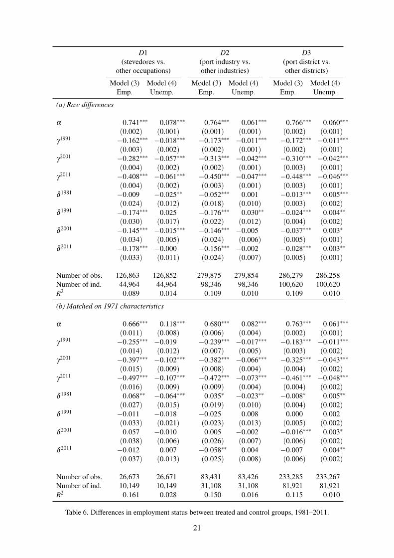
In Tables 6 and 7 we consider outcomes for different employment states. Recall that inour sample everyone in the sample is in employment in 1971. In each successive cen-sus, individuals report their labour market status at the time of the census. For men, fourlabour market states account for the vast majority of observations: employment (includingself-employment), unemployment, retirement, sickness/disability. Models (3)–(6) take eachof these four states as the dependent variable. Precise definitions of each labour marketstate change slightly over the 1981–2011 censuses, and are summarised in Table B1 in Ap-pendix B.

First consider the raw probabilities of each labour market state in 1981, shown in panel(a) of Tables 6 and 7. For sample D1, estimates of α show that 74% of the control groupare in employment, 8% are unemployed, 14% are retired and 3.7% are permanently sick ordisabled. As the sample ages the proportion in employment falls and the proportion retired

20

D1(stevedores vs.

other occupations)



Model (3)Emp.

Model (4)Unemp.

Model (3)Emp.

Model (4)Unemp.

Model (3)Emp.

Model (4)Unemp.

(a) Raw differences

α 0.741∗∗∗ 0.078∗∗∗ 0.764∗∗∗ 0.061∗∗∗ 0.766∗∗∗ 0.060∗∗∗

(0.002) (0.001) (0.001) (0.001) (0.002) (0.001)γ1991 −0.162∗∗∗ −0.018∗∗∗ −0.173∗∗∗ −0.011∗∗∗ −0.172∗∗∗ −0.011∗∗∗

(0.003) (0.002) (0.002) (0.001) (0.002) (0.001)γ2001 −0.282∗∗∗ −0.057∗∗∗ −0.313∗∗∗ −0.042∗∗∗ −0.310∗∗∗ −0.042∗∗∗

(0.004) (0.002) (0.002) (0.001) (0.003) (0.001)γ2011 −0.408∗∗∗ −0.061∗∗∗ −0.450∗∗∗ −0.047∗∗∗ −0.448∗∗∗ −0.046∗∗∗

(0.004) (0.002) (0.003) (0.001) (0.003) (0.001)δ 1981 −0.009 −0.025∗∗ −0.052∗∗∗ 0.001 −0.013∗∗∗ 0.005∗∗∗

(0.024) (0.012) (0.018) (0.010) (0.003) (0.002)δ 1991 −0.174∗∗∗ 0.025 −0.176∗∗∗ 0.030∗∗ −0.024∗∗∗ 0.004∗∗

(0.030) (0.017) (0.022) (0.012) (0.004) (0.002)δ 2001 −0.145∗∗∗ −0.015∗∗∗ −0.146∗∗∗ −0.005 −0.037∗∗∗ 0.003∗

(0.034) (0.005) (0.024) (0.006) (0.005) (0.001)δ 2011 −0.178∗∗∗ −0.000 −0.156∗∗∗ −0.002 −0.028∗∗∗ 0.003∗∗

(0.033) (0.011) (0.024) (0.007) (0.005) (0.001)



α 0.666∗∗∗ 0.118∗∗∗ 0.680∗∗∗ 0.082∗∗∗ 0.763∗∗∗ 0.061∗∗∗

(0.011) (0.008) (0.006) (0.004) (0.002) (0.001)γ1991 −0.255∗∗∗ −0.019 −0.239∗∗∗ −0.017∗∗∗ −0.183∗∗∗ −0.011∗∗∗

(0.014) (0.012) (0.007) (0.005) (0.003) (0.002)γ2001 −0.397∗∗∗ −0.102∗∗∗ −0.382∗∗∗ −0.066∗∗∗ −0.325∗∗∗ −0.043∗∗∗

(0.015) (0.009) (0.008) (0.004) (0.004) (0.002)γ2011 −0.497∗∗∗ −0.107∗∗∗ −0.472∗∗∗ −0.073∗∗∗ −0.461∗∗∗ −0.048∗∗∗

(0.016) (0.009) (0.009) (0.004) (0.004) (0.002)δ 1981 0.068∗∗ −0.064∗∗∗ 0.035∗ −0.023∗∗ −0.008∗ 0.005∗∗

(0.027) (0.015) (0.019) (0.010) (0.004) (0.002)δ 1991 −0.011 −0.018 −0.025 0.008 0.000 0.002

(0.033) (0.021) (0.023) (0.013) (0.005) (0.002)δ 2001 0.057 −0.010 0.005 −0.002 −0.016∗∗∗ 0.003∗

(0.038) (0.006) (0.026) (0.007) (0.006) (0.002)δ 2011 −0.012 0.007 −0.058∗∗ 0.004 −0.007 0.004∗∗

(0.037) (0.013) (0.025) (0.008) (0.006) (0.002)


Table 6. Differences in employment status between treated and control groups, 1981–2011.

21

D1(stevedores vs.

other occupations)



Model (5)Retired

Model (6)Sick

Model (5)Retired

Model (6)Sick

Model (5)Retired

Model (6)Sick

(a) Raw differences

α 0.140∗∗∗ 0.037∗∗∗ 0.140∗∗∗ 0.031∗∗∗ 0.140∗∗∗ 0.031∗∗∗

(0.002) (0.001) (0.001) (0.001) (0.001) (0.001)γ1991 0.132∗∗∗ 0.041∗∗∗ 0.145∗∗∗ 0.033∗∗∗ 0.145∗∗∗ 0.032∗∗∗

(0.002) (0.002) (0.002) (0.001) (0.002) (0.001)γ2001 0.251∗∗∗ 0.078∗∗∗ 0.284∗∗∗ 0.064∗∗∗ 0.281∗∗∗ 0.064∗∗∗

(0.003) (0.002) (0.002) (0.001) (0.002) (0.002)γ2011 0.441∗∗∗ 0.010∗∗∗ 0.476∗∗∗ 0.005∗∗∗ 0.474∗∗∗ 0.006∗∗∗

(0.004) (0.002) (0.003) (0.001) (0.003) (0.001)δ 1981 0.017 0.021 0.036∗∗ 0.018∗∗ 0.006∗∗ 0.002

(0.020) (0.013) (0.015) (0.009) (0.003) (0.001)δ 1991 0.066∗∗ 0.069∗∗∗ 0.076∗∗∗ 0.058∗∗∗ 0.013∗∗∗ 0.007∗∗∗

(0.029) (0.022) (0.022) (0.015) (0.004) (0.002)δ 2001 0.112∗∗∗ 0.060∗ 0.090∗∗∗ 0.050∗∗ 0.031∗∗∗ 0.003

(0.036) (0.031) (0.026) (0.021) (0.005) (0.003)δ 2011 0.191∗∗∗ 0.002 0.174∗∗∗ −0.011 0.026∗∗∗ −0.002

(0.038) (0.019) (0.027) (0.010) (0.006) (0.002)



α 0.148∗∗∗ 0.065∗∗∗ 0.182∗∗∗ 0.052∗∗∗ 0.138∗∗∗ 0.034∗∗∗

(0.008) (0.007) (0.005) (0.003) (0.002) (0.001)γ1991 0.214∗∗∗ 0.043∗∗∗ 0.208∗∗∗ 0.042∗∗∗ 0.149∗∗∗ 0.038∗∗∗

(0.012) (0.010) (0.007) (0.004) (0.003) (0.002)γ2001 0.394∗∗∗ 0.113∗∗∗ 0.369∗∗∗ 0.087∗∗∗ 0.290∗∗∗ 0.073∗∗∗

(0.016) (0.016) (0.008) (0.007) (0.004) (0.003)γ2011 0.589∗∗∗ −0.015 0.541∗∗∗ −0.013∗∗∗ 0.490∗∗∗ 0.005∗∗∗

(0.017) (0.013) (0.009) (0.004) (0.004) (0.002)δ 1981 0.001 −0.002 −0.008 −0.001 0.005 −0.003

(0.021) (0.016) (0.016) (0.009) (0.003) (0.002)δ 1991 −0.019 0.040∗ −0.026 0.030∗ 0.004 −0.006∗∗

(0.033) (0.024) (0.023) (0.015) (0.005) (0.003)δ 2001 −0.045 0.006 −0.033 0.008 0.021∗∗∗ −0.011∗∗∗

(0.041) (0.037) (0.028) (0.023) (0.006) (0.004)δ 2011 0.024 0.004 0.073∗∗∗ −0.012 0.005 −0.003

(0.044) (0.024) (0.028) (0.011) (0.007) (0.003)


Table 7. Differences in retirement and sickness status between treated and control groups,1981–2011.

22

or sick increases, as indicated by the estimates of γs. We observe similar patterns for samplesD2 and D3. There are large differences between the employment patterns of the treatmentand control groups in panel (a). For sample D1, stevedores are are 17pp less likely to bein employment in 1991, 6.6pp more likely to be retired and 6.9pp more likely to be sick ordisabled. A similar picture emerges for sample D2, where port-industry workers are 27.6ppless likely to be in employment, 7.6pp more likely to be retired and 5.8pp more likely tobe sick or disabled. We also see significant differences for sample D3, where the treatmentgroup (those living in port districts) are significantly less likely to be in employment andsignificantly more likely to be retired or sick in 1991.21

Two points are striking about the raw differences in employment outcomes. First, in sam-ple D1, large gaps only emerge from 1991 onwards. In fact, employment rates for stevedoresare insignificantly different from those for the control group (δ 1981 =−0.009 with a standarderror of 0.024); unemployment rates for stevedores are actually 2.5pp lower than the controlgroup. In contrast, a negative employment gap has already emerged in 1981 for samples D2and D3. This result is entirely consistent with the pattern of industrial relations describedin Section 2. The National Dock Labour Scheme prevented any involuntary redundancy forstevedores until 1989. Second, differences in employment outcomes are vary long-lasting,with significant differences in employment rates and retirement rates even up to 2011.

Panel (b) in Tables 6 and 7 repeats the analysis after matching. As before, matchinggreatly changes the composition of the control group. For example, in sample D1 the un-matched control group have an employment rate in 1981 of 0.741; the same employmentrate for the matched control group is 0.666. Similarly, the matched control group have higherrates of unemployment, retirement and disability. As a result the DiD estimates become muchsmaller and in most cases are no longer significantly different from zero. It is particularly no-ticeable that, in sample D1, estimates of δ 1981 are now positive for employment (0.068 witha standard error of 0.027) and negative for unemployment (−0.064 with a standard error of0.015). Employment guarantees clearly worked for stevedores compared to the matched con-trol group. More surprisingly, estimates of δ 1991, δ 2001 and δ 2011 are generally small andinsignificantly different from zero. Overall, employment rates for stevedores and workers inthe port industry were no lower in subsequent years than for the matched control group. Inpart, this reflects the extremely poor employment performance of unskilled men during theperiod, as documented in for example Nickell and Bell (1995).

21One can compare the D3 sample results to the district-level results shown in Section 3. Table 1 shows thatemployment rates were between 4pp and 5pp lower in port districts between 1991 and 2011. Our estimates fromthe individual-level results are similar (2.4pp in 1991 and 3.7pp in 2001).

23

5.3 Geographical and occupational movement

One possible effect of containerisation is to force workers to move to different geographicalareas, or to change occupation. The LS includes an indicator for whether the respondent isliving at a different address as 10 years previously, and we use this as our dependent vari-able for Model (7). Measuring occupational mobility is more complex because of numerouschanges in occupational coding between 1971–2011. However, in each census in the LS(apart from 2011) occupation is coded using the same classification as in the previous census,so for Model (8) we construct an indicator (for those in employment) which takes the value 1if the individual has the same occupation as 10 years previously. Results are in Table 8.

Estimates of α in panel (a) show that about half the control group changed address inthe 10 years between 1971 and 1981. Estimates of γs then show that the probability ofchanging address declines in the control group over each of the following 10 year intervals,which in part reflects the aging of the sample. For example, the probability of changingaddress falls to 38% between 1981 and 1991 (0.519−0.135) and 22% between 2001 and 2011(0.519− 0.296). Similar patterns are observed in the control group for samples D2 and D3.The estimates of δ s in sample D1 are negative, but all insignificantly different from zero. Thisis true both in the raw data (panel a) and after matching (panel b). In other words, stevedoresin 1971 did not exhibit any greater tendency to change address in any of the subsequentdecades up to 2011. Thus, despite the dramatic decline in jobs for stevedores in this period,there appears to have been no additional geographic mobility response at all. This result isconsistent with the well-established result that geographic mobility in response to shocks issmall, in particular among less-skilled workers (e.g. Bound and Holzer, 2000). In sample D2there is some evidence of lower geographic mobility (estimates of δ s are all negative), butthis effect largely disappears in panel (b) after matching. In sample D3 there does not appearto be a consistent difference between the treatment and control group after matching: wefind somewhat lower mobility rates between 1971 and 1981 (δ 1981 =−0.01), but somewhathigher rates between 1991 and 2001 (δ 2001 = 0.013). These effects are also very small whencompared to the proportion of the control group who move. Thus overall we find no evidenceof increased mobility as a result of the dramatic reductions in port employment.

Finally in Model (8) we consider occupational mobility. The sample here consists onlyof individuals who are observed in employment in consecutive censuses, and the dependentvariable takes the value one if individuals are in the same three-digit occupation and zerootherwise. This variable is not available in 2011 because of changes to occupational defini-tions. Changes in occupation are very common: in the control group only 38% of the samplehave the same occupation in 1971 and 1981 (α = 0.381), and this increases slightly to 45%between 1981 and 1991 and 40% between 1991 and 2001. As we would expect, for samplesD1 and D2 there is a very strong effect of containerisation on occupation, but again tempered

24

D1(stevedores vs.

other occupations)



Model (7)Moved in

last 10years

Model (8)Same occ.

in last10 years

Model (7)Moved in

last 10years

Model (8)Same occ.

in last10 years

Model (7)Moved in

last 10years

Model (8)Same occ.

in last10 years

(a) Raw differences

α 0.519∗∗∗ 0.381∗∗∗ 0.553∗∗∗ 0.373∗∗∗ 0.551∗∗∗ 0.370∗∗∗

(0.002) (0.003) (0.002) (0.002) (0.002) (0.002)γ1991 −0.135∗∗∗ 0.074∗∗∗ −0.134∗∗∗ 0.070∗∗∗ −0.131∗∗∗ 0.070∗∗∗

(0.003) (0.004) (0.002) (0.003) (0.002) (0.003)γ2001 −0.231∗∗∗ 0.015∗∗∗ −0.245∗∗∗ 0.002 −0.245∗∗∗ 0.006

(0.004) (0.005) (0.002) (0.004) (0.003) (0.004)γ2011 −0.296∗∗∗ −0.320∗∗∗ −0.318∗∗∗

(0.004) (0.003) (0.003)δ 1981 −0.022 0.167∗∗∗ −0.072∗∗∗ 0.137∗∗∗ 0.003 0.031∗∗∗

(0.027) (0.031) (0.020) (0.024) (0.004) (0.005)δ 1991 −0.016 −0.147∗∗∗ −0.070∗∗∗ −0.057 −0.014∗∗∗ 0.018∗∗∗

(0.030) (0.045) (0.022) (0.035) (0.005) (0.006)δ 2001 −0.035 0.104 −0.057∗∗ 0.050 0.008 0.001

(0.032) (0.072) (0.023) (0.052) (0.005) (0.008)δ 2011 −0.003 −0.003 −0.006

(0.039) (0.028) (0.005)



α 0.524∗∗∗ 0.299∗∗∗ 0.513∗∗∗ 0.346∗∗∗ 0.564∗∗∗ 0.374∗∗∗

(0.012) (0.014) (0.006) (0.006) (0.003) (0.003)γ1991 −0.176∗∗∗ 0.104∗∗∗ −0.147∗∗∗ 0.083∗∗∗ −0.151∗∗∗ 0.071∗∗∗

(0.016) (0.022) (0.008) (0.010) (0.004) (0.005)γ2001 −0.228∗∗∗ 0.088∗∗∗ −0.220∗∗∗ 0.022∗ −0.264∗∗∗ 0.005

(0.018) (0.026) (0.008) (0.012) (0.004) (0.006)γ2011 −0.279∗∗∗ −0.283∗∗∗ −0.335∗∗∗

(0.019) (0.010) (0.004)δ 1981 −0.020 0.243∗∗∗ −0.034 0.162∗∗∗ −0.010∗∗ 0.015∗∗∗

(0.030) (0.036) (0.021) (0.025) (0.005) (0.005)δ 1991 0.021 −0.112∗∗ −0.013 −0.052 −0.004 0.013∗

(0.034) (0.050) (0.023) (0.037) (0.005) (0.007)δ 2001 −0.048 0.090 −0.043∗ 0.041 0.013∗∗ −0.009

(0.037) (0.079) (0.025) (0.053) (0.006) (0.009)δ 2011 −0.005 0.008 −0.001

(0.046) (0.030) (0.006)


Table 8. Differences in geographical and occupational mobility between treated and control groups,1981–2011

25

by the effect of employment protection. For both samples D1 and D2 the treatment group aremore likely to remain in the same occupation between 1971 and 1981 (δ 1981 = 0.243 in D1and 0.162 in D2). This switches to a large negative effect for stevedores between 1981 and1991 (δ 1991 = −0.112 in D1) which is consistent with the fact that employment guaranteeswere removed in 1989 (see Section 2). It is noticeable that the negative occupational effectin 1991 is much weaker for sample D2, suggesting that port industry workers as a wholewere less affected by the new technology than stevedores in particular. The hypothesis thatstevedores or port workers were subsequently sorted into less stable jobs is not borne out.Estimates of δ 2001 are insignificantly different from zero for both D1 and D2, showing thatthe change in occupations which occurred between 1981 and 1991 did not continue. Theresults for sample D3 suggest that wide geographical effects are much weaker.

5.4 Robustness checks

In this section we consider a number of sub-samples to examine whether our results are ro-bust. First, we consider whether the effects of containerisation on stevedores differ accordingto their initial socio-economic group. Socio-economic group is determined by a combinationof occupation and employment status (Hattersley and Creeser, 1995). Unskilled workers whohave some supervisory role (foremen) are classified as “skilled manual”; Table 3 shows that23% of stevedores are classified as skilled manual. In Table C5 we report PSM estimates ofModels (1)–(8) for just those stevedores who have no supervisory role i.e. the less skilled, orless senior. These results show that outcomes for these less-skilled stevedores were no worsethan for stevedores overall, and in many cases actually more favourable. The treatment groupare still more likely to appear in the linked census in subsequent years, they have lower mor-tality rates, higher employment rates and lower unemployment rates in 1981. Thus, it appearsthat the employment guarantees in place protected all stevedores and not just those in moresenior positions. Indeed, the results from model (8) show that the probability of remaining inthe same occupation was even higher for the less-skilled stevedores in 1981 (δ 1981 = 0.261in the final column of Table C5) than for the the whole treatment group (δ 1981 = 0.243 inTable 8).

Our second robustness check modifies sample D2 so that it excludes stevedores. Thetreatment group in this case therefore consists of workers who worked in the port industry in1971 but who were not stevedores. A comparison of this restricted sample with sample D2allows us to confirm that the employment guarantee protected stevedores far more than otherworkers in the port industry. Results for Models (1)–(8) are shown in Table C6. Recall thatour estimate of δ 1981 for Model (2) was positive in 1981, showing that port workers actuallyhad higher employment rates than the control group in 1981 (see Table 6). However, in themodified sample δ 1981 = 0.006 and is insignificantly different from zero.

26

Our third robustness check considers in more detail the geographical comparisons ofsample D3. In Table C7 we restrict the control group to include workers in Counties whichcontain no major ports, while in Table C8 we restrict the control group to include workerswho work in districts which are more than 20km from any port. We do this because it seemsthat the basic geographic control group D3 = 0 may include workers who are affected bythe process of containerisation because their place of work is near a port, even if it not ina district which includes a port. Results from Tables C7 and C8 show some evidence ofnegative employment effects (and positive unemployment effects) in 1981, but the size ofthese effects are still small compared to those from a comparison of occupation and industry.

6 Conclusion

Containerisation provides us with an opportunity to examine the labour market consequencesof a technological shock which, in the space of a few years, completely removed the demandfor a particular occupation. Linked census data enables us to track the workers in affectedoccupations and industries over the long-run, and to shed light on the process of adjustment.We have documented that stevedores and the port industry did suffer massive falls in demandfor labour between the late 1960s and early 1980s. We have also shown that the districts con-taining ports experienced worse labour market outcomes which continued and have remainedfor over 30 years.

However, our worker-level analysis reveals a different picture. After matching stevedoresand port-industry workers to observably similar unskilled men in other occupations and in-dustries, we find that subsequent differences in labour market outcomes, mortality and mo-bility are typically small, insignificantly different from zero and even in some cases positive.Positive differences are most notable in 1981, at which point stevedores were protected fromredundancy by the National Dock Labour Scheme. Perhaps more surprisingly, even after em-ployment protection was removed there are not large differences in labour market outcomesbetween the treatment and control groups. Thus, we can conclude that workers who werestevedores or who worked in the port industry in 1971 did not suffer long-term disadvantagein the labour market over the rest of their working lives.

This result should be interpreted in the light of the unique industrial relations policieswhich existed for this particular group of workers at the time of the shock. Dock workerswere insulated from redundancy for a long time after the technological shock. This itself hadconsequences for the development of new ports in the UK, such that port activity shifted andconcentrated in entirely new locations. One might therefore be concerned that the employ-ment protection merely delayed and possibly amplified the eventual costs in terms of lostjobs. However, this does not appear to be the case because our estimates for 1991–2011 are

27

also typically small or insignificant for all employment outcomes and for mortality.

There are several important caveats. First, we recognise that the process of containeri-sation and the associated fall in demand for stevedores began before 1971. Unfortunately,linked census data before 1971 is not available. Our treatment group is therefore a selectedsample of workers who remained in that occupation or industry even after it became apparentthat their work was changing and their jobs disappearing. However, one might argue that thiswould bias our results towards finding large negative subsequent labour market outcomes ifthose workers who did not have better outside opportunities were the ones to remain in 1971.

Second, is it possible that the adjustment process is fast enough that our 10-year intervalsfrom census data miss much of the effect? The existing literature on displaced workers sug-gests not. Although the literature typically regards the “long-run” as being within 10 yearsof job loss, the consensus is that losses are still evident at that point. However, results fromthe US suggest that most of these losses come in the form of wages rather than employmentdifferentials. It therefore seems possible that the men in our sample are suffering wage lossesrather than employment losses.22

The final issue is the extent to which one can regard the various control groups we useas suitable counterfactuals for the treatment group. A profound technological shock suchas the invention of containers may have had consequences far beyond the narrow treatmentand control groups as defined here. For example, containerisation may have had a role toplay in the growth in world trade which occurred over this period (Bernhofen et al., 2013)which itself affected labour market outcomes more generally (Autor et al., 2014). It is well-known that unskilled workers in general had extremely poor labour market outcomes duringthe 1980s and 1990s (Nickell and Bell, 1995), and this is clear in the estimated effects for ourcontrol group. Our final conclusion must therefore be that stevedores and workers in the portindustry fared “no worse” than similar workers in other occupations and industries, ratherthan actually doing well.

22There is no wage information in the LS.

28

References

Autor, D., Dorn, D., Hanson, G. and Song, J. (2014), “Trade adjustment: worker-level evi-dence”, Quarterly Journal of Economics 129(4), 1799–1860.

Bernhofen, D. M., El-Sahli, Z. and Kneller, R. (2013), “Estimating the effects of the containerrevolution on world trade”, GEP working paper 13/02.

Black, D., Daniel, K. and Sanders, S. (2002), “The impact of economic conditions on partici-pation in disability programs: Evidence from the coal boom and bust”, American Economic

Review 92(1), 27–50.

Black, D., McKinnish, T. and Sanders, S. (2005), “The economic impact of the coal boomand bust”, The Economic Journal 115(503), 449–476.

Black, S., Devereux, P. and Salvjanes, K. (2012), “The effect of job displacement on health”,NBER working paper 18660.

Bound, J. and Holzer, H. J. (2000), “Demand shifts, population adjustments, and labor marketoutcomes during the 1980s”, Journal of Labor Economics 18(1), 20–54.

Cameron, C. and Trivedi, P. (2005), Microeconometrics: methods and applications, Cam-bridge: Cambridge University Press.

Central Statistical Office (1970), “Standard industrial classification”. London: Her Majesty’sStationary Office.

Couch, K. A. and Placzek, D. W. (2010), “Earnings losses of displaced workers revisited”,The American Economic Review 100(1), 572–589.

Davis, S. J. and von Wachter, T. (2011), “Recessions and the costs of job loss”, Brookings

Papers on Economic Activity Fall, 1–55.

El-Sahli, Z. (2012), “Estimating the effects of containerisation on world trade”, PhD thesis,School of Economics, University of Nottingham.

Eliason, M. (2012), “Lost jobs, broken marriages”, Journal of Population Economics

25, 1365–1397.

Eliason, M. and Storrie, D. (2009), “Does job loss shorten life?”, Journal of Human Re-

sources 44(2), 277–302.

Fieldhouse, E. and Hollywood, E. (1999), “Life after mining: Hidden unemployment andchanging patterns of economic activity amongst miners in England and Wales, 1981-1991”,Work, Employment & Society 13(3), 483–502.

29

Hall, P. (2009), “Container ports, local benefits and transportation worker earnings”, Geo-

Journal 74(1), 67–83.

Hattersley, L. and Creeser, R. (1995), “Longitudinal study 1971–1991: history, organisationand quality of the data”, OPCS working paper LS 7.

Hinde, K. (1994), “Labour market experiences following plant closure: the case of Sunder-land’s shipyard workers”, Regional Studies 28(7), 713–724.

Hoare, A. G. (1986), “British ports and their export hinterlands: A rapidly changing geogra-phy”, Geografiska Annaler. Series B, Human Geography 68(1), pp. 29–40.

Jacobson, L. S., LaLonde, R. J. and Sullivan, D. G. (1993), “Earnings losses of displacedworkers”, The American Economic Review 83(4), 685–709.

Levinson, M. (2006), The Box: How the Shipping Container Made the World Smaller and

the World Economy Bigger, Princeton University Press.

Lindsay, C. and Doyle, P. (2003), “Experimental consistent time series of historical labourforce survey data”, Labour Market Trends 467–475.

McVicar, D. (2008), “Why have UK disability benefit rolls grown so much?”, Journal of

Economic Surveys 22(1), 114–139.

Nickell, S. and Bell, B. (1995), “The collapse in demand for the unskilled and unemploymentacross the OECD”, Oxford Review of Economic Policy 11, 40–62.

Office for Population Censuses and Surveys (1970), “Classification of occupations 1970”.London: Her Majesty’s Stationary Office.

Picard, R. (2010), “GEODIST: Stata module to compute geodetic distances”, Statistical Soft-ware Components, Boston College Department of Economics.URL: http://ideas.repec.org/c/boc/bocode/s457147.html

Rosenbaum, P. and Rubin, D. (1983), “The central role of the propensity score in observa-tional studies for causal effects”, Biometrika 70(1), 41–55.

Ruhm, C. (1991), “Are workers permanently scarred by job displacements?”, American Eco-

nomic Review 81, 319–324.

Talley, W. (2002), “Dockworker earnings, containerisation, and shipping deregulation”, Jour-

nal of Transport Economics and Policy 36(3), 447–467.

Turnbull, P. (1992), “Dock strikes and the demise of the dockers’ occupational culture”, So-

ciological Review 40(2), 294 – 318.

30

Turnbull, P. (2012), “Port labor”, in W. K. Talley, ed., The Blackwell Companion to Maritime

Economics, Wiley-Blackwell, chapter 26, 517–548.

Turnbull, P., Morris, J. and Sapsford, D. (1996), “Persistent militants and quiescent comrades:intra-industry strike activity on the docks, 1947-89.”, Sociological Review 44(4), 692 – 727.

Turnbull, P. and Wass, V. (1994), “The greatest game no more — redundant dockers and thedemise of dock work”, Work, Employment & Society 8(4), 487–506.

Upward, R. and Wright, P. (2013), “Coping with job loss: new evidence from householdsurvey data”, Mimeo, University of Nottingham.

Vigarie, A. (1999), “From break-bulk to containers: the transformation of general cargo han-dling and trade”, GeoJournal 48(1), 3–7.

31

Appendix A Port locations

Major PortForeign

Tonnage(000s)

Est. portemployment

Est. no.stevedores

London (inc. Tilbury) 35,150 38,600 13,280Liverpool 22,687 29,330 13,470Medway and Dover 21,747 2,940 1,180Milford Haven 19,807 440 190Southampton 17,092 4,420 2,260Manchester 10,898 4,900 1,830Tees and Hartlepool 9,080 2,240 1,060Hull 5,519 8,780 4,520Immingham 5,472 3,290 1,820Bristol 4,248 4,410 1,750Newport 3,865 1,300 680Port Talbot 3,360 410 230Swansea 2,936 2,000 730Tyne 2,551 2,060 850Cardiff 1,940 1,870 580Par and Fowey 1,524 1,190 200Felixstowe 1,118 400 130Goole 837 1,600 410Harwich 817 780 410Grimsby 792 2,550 1,300Preston 762 840 320Whitehaven and Workington 757 310 160Great Yarmouth 691 370 120Ipswich 635 240 60Boston 539 310 220Plymouth 519 900 180Shoreham 470 180 30King’s Lynn 449 310 220Teignmouth 326 130 60Holyhead 262 160 10Barrow 172 250 50

All major ports above 177,022 117,510 48,310All ports England and Wales 185,904 132,750 59,190

Table A1. Major English and Welsh ports by tonnage, 1967 and employment, 1961. Major ports arethose listed individually in the Digest of Port Statistics, 1968. Employment is estimated from 10%published census tables, based on recorded employment in the Local Government Districts whichcontained a major port.

32

Major Port Local authorities (1961) Local authorities (1971)

London (inc. Tilbury) City of London, Poplar, Stepney, WestHam, East Ham, Barking, Dagenham,Hornchurch, Southwark, Bermondsey,Deptford, Greenwich, Woolwich, Erith,Crayford, Thurrock

Barking, Bexley, City of London,Greenwich, Havering, Lewisham,Newham, Southwark, Tower Hamlets,Thurrock (Tilbury), Gravesend(Tilbury),

Liverpool Bootle, Crosby, Birkenhead, Wallesey,Bebington, Liverpool

Bebington, Birkenhead, Bootle, Crosby,Ellesmere Port, Liverpool, Runcorn,Wallasey

Medway and Dover Kent (county remainder) Gillingham, Chatham, Rochester,Queenborough-in-Sheppey

Milford Haven Pembrokeshire Milford Haven, PembrokeSouthampton Southampton SouthamptonManchester Salford, Manchester, Stretford Salford, Manchester, StretfordTees and Hartlepool Middlesbrough Hartlepool, TeessideHull Kingston-upon-Hull Kingston-up-HullImmingham Lincolnshire (parts of Lindsey) GrimsbyBristol Bristol BristolNewport Newport NewportPort Talbot Port Talbot Port TalbotSwansea Swansea SwanseaTyne Tynemouth South Shields, TynemouthCardiff Cardiff CardiffPar and Fowey Cornwall and the Isles of Scilly St Austell with FoweyFelixstowe Suffolk FelixstoweDover Kent (county remainder) DoverGoole Yorkshire West Riding (county

remainder)Goole

Harwich Essex (county remainder) Harwich, TendringGrimsby Grimsby GrimsbyPreston Preston PrestonWorkington Cumberland WorkingtonWhitehaven Cumberland WhitehavenGreat Yarmouth Great Yarmouth Great YarmouthIpswich Ipswich IpswichBoston Lincolnshire (parts of Holland) BostonPlymouth Plymouth PlymouthShoreham Sussex (county remainder) Shoreham-by-Sea, SouthwickKing’s Lynn Norfolk King’s LynnTeignmouth Devon (county remainder) TeignmouthHolyhead Anglesey HolyheadBarrow Barrow-in-Furness Barrow-in-Furness

Table A2. Local authority areas classified as containing a major port in 1961 and 1971.

33

Appendix B Definition of labour market states

1981 1991 2001 2011

Employed In a full- orpart-time job atany time in the lastweek

Employed orself-employed inthe last week

Same as 1991 Same as 2001

Unemployed Waiting to take upjob or seeking job

Waiting to start jobor seeking job

Not working,actively lookingfor paid work inlast four weeksand available tostart within twoweeks; or waitingto start job

Same as 2001

Retired Wholly retiredfrom employment

Retired from paidwork

Retired Retired (whetherreceiving pensionor not)

Sick Permanently sickor disabled

Unable to workbecause of longterm sickness ordisability

Permanentlysick/disabled

Long-term sick ordisabled

Table B1. Definition of labour market states 1981–2011.

34

Appendix C Additional results

D1(stevedores vs.

other occupations)



In census Died In census Died In census Died

γ1991 −0.136∗∗∗ 0.142∗∗∗ −0.131∗∗∗ 0.136∗∗∗ −0.131∗∗∗ 0.136∗∗∗

(0.002) (0.002) (0.001) (0.001) (0.001) (0.001)γ2001 −0.297∗∗∗ 0.313∗∗∗ −0.288∗∗∗ 0.303∗∗∗ −0.288∗∗∗ 0.303∗∗∗

(0.002) (0.002) (0.002) (0.001) (0.002) (0.002)γ2011 −0.437∗∗∗ 0.470∗∗∗ −0.428∗∗∗ 0.459∗∗∗ −0.429∗∗∗ 0.459∗∗∗

(0.002) (0.002) (0.002) (0.002) (0.002) (0.002)δ 1981 0.143∗∗∗ −0.086∗∗∗ 0.107∗∗∗ −0.064∗∗∗ 0.008∗∗∗ −0.006∗∗

(0.018) (0.015) (0.014) (0.012) (0.003) (0.002)δ 1991 0.094∗∗∗ −0.052∗∗∗ 0.057∗∗∗ −0.023∗ 0.007∗∗ −0.004

(0.021) (0.019) (0.015) (0.014) (0.003) (0.003)δ 2001 0.046∗∗ −0.017 0.027∗ 0.005 0.004 −0.002

(0.022) (0.021) (0.015) (0.015) (0.003) (0.003)δ 2011 0.022 0.022 −0.001 0.033∗∗ 0.006∗ −0.002

(0.021) (0.021) (0.014) (0.014) (0.003) (0.003)


Table C1. OLS estimates of differences in attrition rates and mortality between treated and controlgroups, 1981–2011. These results can be compared to the propensity-score matching estimatesshown in the bottom panel of Table 5.

35

D1(stevedores vs.

other occupations)



Emp. Unemp. Emp. Unemp. Emp. Unemp.

γ1991 −0.225∗∗∗ −0.023∗∗∗ −0.234∗∗∗ −0.014∗∗∗ −0.234∗∗∗ −0.014∗∗∗

(0.003) (0.002) (0.002) (0.001) (0.002) (0.001)γ2001 −0.429∗∗∗ −0.067∗∗∗ −0.456∗∗∗ −0.049∗∗∗ −0.453∗∗∗ −0.049∗∗∗

(0.003) (0.002) (0.002) (0.001) (0.002) (0.001)γ2011 −0.632∗∗∗ −0.076∗∗∗ −0.669∗∗∗ −0.057∗∗∗ −0.668∗∗∗ −0.057∗∗∗

(0.003) (0.002) (0.002) (0.001) (0.003) (0.001)δ 1981 0.151∗∗∗ −0.055∗∗∗ 0.085∗∗∗ −0.014 0.004 0.004∗

(0.020) (0.012) (0.015) (0.010) (0.003) (0.002)δ 1991 −0.019 −0.003 −0.052∗∗∗ 0.012 −0.006∗ 0.002

(0.024) (0.017) (0.018) (0.012) (0.003) (0.002)δ 2001 0.032 −0.045∗∗∗ −0.031 −0.022∗∗∗ −0.020∗∗∗ 0.001

(0.029) (0.006) (0.020) (0.007) (0.004) (0.002)δ 2011 −0.002 −0.027∗∗ −0.047∗∗ −0.017∗∗ −0.008 0.001

(0.030) (0.012) (0.022) (0.008) (0.005) (0.002)


Table C2. OLS estimates of differences in employment status between treated and control groups,1981–2011. These results can be compared to the propensity-score matching estimates shown in thebottom panel of Table 6.

D1(stevedores vs.

other occupations)



Retired Sick Retired Sick Retired Sick

γ1991 0.202∗∗∗ 0.040∗∗∗ 0.211∗∗∗ 0.033∗∗∗ 0.211∗∗∗ 0.032∗∗∗

(0.002) (0.002) (0.001) (0.001) (0.002) (0.001)γ2001 0.412∗∗∗ 0.080∗∗∗ 0.437∗∗∗ 0.066∗∗∗ 0.433∗∗∗ 0.066∗∗∗

(0.003) (0.002) (0.002) (0.001) (0.002) (0.002)γ2011 0.684∗∗∗ 0.013∗∗∗ 0.708∗∗∗ 0.009∗∗∗ 0.707∗∗∗ 0.009∗∗∗

(0.003) (0.002) (0.002) (0.001) (0.002) (0.001)δ 1981 −0.072∗∗∗ −0.017 −0.057∗∗∗ −0.010 −0.002 −0.006∗∗∗

(0.015) (0.013) (0.011) (0.009) (0.002) (0.002)δ 1991 −0.022 0.031 −0.004 0.031∗∗ 0.004 −0.000

(0.019) (0.022) (0.014) (0.015) (0.003) (0.002)δ 2001 0.011 0.018 0.023 0.022 0.023∗∗∗ −0.006∗

(0.027) (0.033) (0.020) (0.021) (0.004) (0.003)δ 2011 0.086∗∗ −0.040∗∗ 0.109∗∗∗ −0.038∗∗∗ 0.016∗∗∗ −0.010∗∗∗

(0.036) (0.020) (0.025) (0.011) (0.005) (0.002)


Table C3. OLS estimates of differences in retirement and sickness status between treated and controlgroups, 1981–2011. These results can be compared to the propensity-score matching estimatesshown in the bottom panel of Table 7.

36

D1(stevedores vs.

other occupations)



Moved inlast 10years

Same occ.in last

10 years


Same occ.in last

10 years


Same occ.in last

10 years

γ1991 −0.151∗∗∗ 0.083∗∗∗ −0.150∗∗∗ 0.081∗∗∗ −0.147∗∗∗ 0.081∗∗∗

(0.003) (0.004) (0.002) (0.003) (0.002) (0.003)γ2001 −0.274∗∗∗ 0.044∗∗∗ −0.288∗∗∗ 0.032∗∗∗ −0.288∗∗∗ 0.037∗∗∗

(0.004) (0.006) (0.002) (0.004) (0.003) (0.004)γ2011 −0.375∗∗∗ −0.398∗∗∗ −0.396∗∗∗

(0.004) (0.003) (0.003)δ 1981 0.003 0.247∗∗∗ −0.028 0.166∗∗∗ 0.001 0.022∗∗∗

(0.027) (0.032) (0.020) (0.024) (0.004) (0.005)δ 1991 0.010 −0.060 −0.024 −0.025 −0.016∗∗∗ 0.012∗

(0.031) (0.048) (0.022) (0.036) (0.005) (0.006)δ 2001 −0.013 0.162∗∗ −0.018 0.076 0.005 −0.006

(0.033) (0.074) (0.024) (0.052) (0.005) (0.008)δ 2011 0.043 0.047 −0.006

(0.040) (0.030) (0.005)


Table C4. OLS estimates of differences in geographical and occupational mobility between treatedand control groups, 1981–2011. These results can be compared to the propensity-score matchingestimates shown in the bottom panel of Table 8.

37

Mod

el(1

)In

cens

usM

odel

(2)

Die

dM

odel

(3)

Em

p.M

odel

(4)

Une

mp.

Mod

el(5

)R

etir

edM

odel

(6)

Sick

Mod

el(7

)M

oved

inla

st10

year

s

Mod

el(8

)Sa

me

occ.

inla

st10

year

s

Mat

ched

on19

71ch

arac

teri

stic

s

α0.

749∗∗∗

0.10

4∗∗∗

0.62

3∗∗∗

0.13

7∗∗∗

0.16

2∗∗∗

0.07

5∗∗∗

0.53

4∗∗∗

0.23

9∗∗∗

(0.0

10)

(0.0

06)

(0.0

15)

(0.0

11)

(0.0

10)

(0.0

10)

(0.0

15)

(0.0

20)

γ19

91−

0.17

0∗∗∗

0.19

3∗∗∗−

0.25

6∗∗∗−

0.01

90.

213∗∗∗

0.04

2∗∗∗−

0.18

2∗∗∗

0.13

4∗∗∗

(0.0

12)

(0.0

11)

(0.0

18)

(0.0

17)

(0.0

16)

(0.0

13)

(0.0

22)

(0.0

33)

γ20

01−

0.37

5∗∗∗

0.43

3∗∗∗−

0.37

1∗∗∗−

0.11

9∗∗∗

0.36

7∗∗∗

0.13

4∗∗∗−

0.22

8∗∗∗

0.13

6∗∗∗

(0.0

14)

(0.0

14)

(0.0

21)

(0.0

12)

(0.0

23)

(0.0

23)

(0.0

24)

(0.0

39)

γ20

11−

0.51

5∗∗∗

0.61

8∗∗∗−

0.46

6∗∗∗−

0.12

5∗∗∗

0.56

8∗∗∗−

0.01

4−

0.28

0∗∗∗

(0.0

14)

(0.0

13)

(0.0

22)

(0.0

12)

(0.0

24)

(0.0

18)

(0.0

27)

δ19

810.

130∗∗∗−

0.03

3∗0.

092∗∗∗−

0.07

8∗∗∗−

0.00

6−

0.00

4−

0.03

80.

261∗∗∗

(0.0

22)

(0.0

17)

(0.0

33)

(0.0

19)

(0.0

26)

(0.0

19)

(0.0

36)

(0.0

43)

δ19

910.

100∗∗∗−

0.04

10.

014

−0.

041

−0.

016

0.03

50.

021

−0.

081

(0.0

31)

(0.0

29)

(0.0

39)

(0.0

26)

(0.0

39)

(0.0

28)

(0.0

40)

(0.0

63)

δ20

010.

095∗∗∗−

0.06

8∗∗

0.06

3−

0.01

0−

0.00

9−

0.03

1−

0.05

60.

094

(0.0

33)

(0.0

34)

(0.0

44)

(0.0

08)

(0.0

49)

(0.0

45)

(0.0

44)

(0.0

95)

δ20

110.

050∗

−0.

033

−0.

040

0.01

40.

036

0.01

60.

010

(0.0

29)

(0.0

32)

(0.0

40)

(0.0

18)

(0.0

53)

(0.0

34)

(0.0

57)

Num

bero

fobs

.22

,108

20,1

5510

,767

10,7

6510

,764

10,3

5610

,205

4,04

9N

umbe

rofi

nd.

5,52

75,

204

4,36

04,

360

4,36

04,

358

4,24

52,

529

R2

0.18

60.

229

0.15

80.

033

0.17

00.

022

0.04

70.

053

Tabl

eC

5.D

iffer

ence

sin

outc

omes

betw

een

stev

edor

esan

dm

atch

edco

ntro

lgro

up,1

981–

2011

.The

sere

sults

are

base

don

sam

ple

D1,

rest

rict

edto

incl

ude

only

wor

kers

clas

sifie

das

bein

gin

the

“uns

kille

d”so

cio-

econ

omic

grou

p.C

ontr

astw

ithco

lum

nD

1in

Tabl

es5,

6an

d7,

whi

chin

clud

esw

orke

rsin

unsk

illed

and

skill

edm

anua

lso

cio-

econ

omic

grou

ps.

38

Mod

el(1

)In

cens

usM

odel

(2)

Die

dM

odel

(3)

Em

p.M

odel

(4)

Une

mp.

Mod

el(5

)R

etir

edM

odel

(6)

Sick

Mod

el(7

)M

oved

inla

st10

year

s

Mod

el(8

)Sa

me

occ.

inla

st10

year

s

Mat

ched

on19

71ch

arac

teri

stic

s

α0.

801∗∗∗

0.11

1∗∗∗

0.68

5∗∗∗

0.06

3∗∗∗

0.20

6∗∗∗

0.04

4∗∗∗

0.50

1∗∗∗

0.38

4∗∗∗

(0.0

03)

(0.0

03)

(0.0

04)

(0.0

02)

(0.0

04)

(0.0

02)

(0.0

04)

(0.0

05)

γ19

91−

0.17

4∗∗∗

0.18

7∗∗∗−

0.22

4∗∗∗−

0.01

5∗∗∗

0.20

1∗∗∗

0.03

1∗∗∗−

0.12

7∗∗∗

0.06

2∗∗∗

(0.0

04)

(0.0

03)

(0.0

05)

(0.0

03)

(0.0

05)

(0.0

03)

(0.0

06)

(0.0

07)

γ20

01−

0.36

8∗∗∗

0.39

9∗∗∗−

0.37

5∗∗∗−

0.04

7∗∗∗

0.36

0∗∗∗

0.06

7∗∗∗−

0.21

0∗∗∗−

0.02

1∗∗

(0.0

04)

(0.0

04)

(0.0

06)

(0.0

02)

(0.0

06)

(0.0

04)

(0.0

06)

(0.0

10)

γ20

11−

0.51

8∗∗∗

0.57

5∗∗∗−

0.46

2∗∗∗−

0.05

4∗∗∗

0.51

1∗∗∗−

0.01

1∗∗∗−

0.27

0∗∗∗

(0.0

04)

(0.0

04)

(0.0

07)

(0.0

02)

(0.0

07)

(0.0

03)

(0.0

07)

δ19

810.

030

0.01

00.

006

0.00

2−

0.00

60.

000

−0.

042

0.05

8∗

(0.0

19)

(0.0

16)

(0.0

25)

(0.0

14)

(0.0

22)

(0.0

11)

(0.0

27)

(0.0

33)

δ19

910.

024

0.00

7−

0.02

50.

023

−0.

024

0.01

9−

0.03

0−

0.02

2(0.0

24)

(0.0

23)

(0.0

31)

(0.0

16)

(0.0

30)

(0.0

18)

(0.0

30)

(0.0

48)

δ20

010.

051∗∗−

0.02

4−

0.03

70.

004

−0.

005

0.00

6−

0.03

4−

0.02

4(0.0

25)

(0.0

25)

(0.0

32)

(0.0

10)

(0.0

36)

(0.0

26)

(0.0

32)

(0.0

68)

δ20

110.

027

−0.

019

−0.

074∗∗−

0.00

10.

095∗∗∗−

0.02

5∗∗∗

0.00

5(0.0

23)

(0.0

24)

(0.0

32)

(0.0

08)

(0.0

35)

(0.0

08)

(0.0

39)

Num

bero

fobs

.11

4,71

210

7,40

363

,769

63,7

6663

,764

60,7

0561

,268

28,5

75N

umbe

rofi

nd.

28,6

7827

,593

24,1

5324

,153

24,1

5324

,145

23,7

6316

,746

R2

0.15

40.

184

0.14

30.

013

0.15

80.

017

0.04

00.

005

Tabl

eC

6.D

iffer

ence

sin

outc

omes

betw

een

stev

edor

esan

dm

atch

edco

ntro

lgro

up,1

981–

2011

.The

sere

sults

are

base

don

sam

ple

D2,

rest

rict

edso

that

the

trea

tmen

tgro

upin

clud

eson

lyw

orke

rsin

the

port

indu

stry

who

are

nots

teve

dore

s.C

ontr

astw

ithco

lum

nD

2in

Tabl

es5,

6an

d7,

whi

chin

clud

esal

lwor

kers

inpo

rtin

dust

ries

inth

etr

eatm

entg

roup

.

39

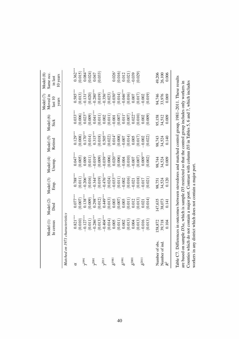
Mod

el(1

)In

cens

usM

odel

(2)

Die

dM

odel

(3)

Em

p.M

odel

(4)

Une

mp.

Mod

el(5

)R

etir

edM

odel

(6)

Sick

Mod

el(7

)M

oved

inla

st10

year

s

Mod

el(8

)Sa

me

occ.

inla

st10

year

s

Mat

ched

on19

71ch

arac

teri

stic

s

α0.

821∗∗∗

0.07

7∗∗∗

0.78

8∗∗∗

0.04

7∗∗∗

0.12

9∗∗∗

0.03

3∗∗∗

0.58

5∗∗∗

0.36

2∗∗∗

(0.0

10)

(0.0

07)

(0.0

11)

(0.0

05)

(0.0

08)

(0.0

06)

(0.0

13)

(0.0

15)

γ19

91−

0.12

7∗∗∗

0.13

8∗∗∗−

0.20

6∗∗∗

0.00

90.

170∗∗∗

0.02

3∗∗−

0.13

1∗∗∗

0.08

4∗∗∗

(0.0

11)

(0.0

09)

(0.0

16)

(0.0

11)

(0.0

14)

(0.0

09)

(0.0

20)

(0.0

24)

γ20

01−

0.28

6∗∗∗

0.29

8∗∗∗−

0.34

4∗∗∗−

0.01

9∗∗

0.31

5∗∗∗

0.04

1∗∗∗−

0.28

0∗∗∗

0.04

7(0.0

13)

(0.0

12)

(0.0

19)

(0.0

09)

(0.0

18)

(0.0

11)

(0.0

19)

(0.0

33)

γ20

11−

0.40

4∗∗∗

0.44

9∗∗∗−

0.47

6∗∗∗−

0.03

9∗∗∗

0.50

5∗∗∗

0.00

2−

0.35

6∗∗∗

(0.0

14)

(0.0

13)

(0.0

24)

(0.0

06)

(0.0

22)

(0.0

11)

(0.0

23)

δ19

810.

005

0.00

3−

0.03

3∗∗∗

0.02

0∗∗∗

0.01

4∗−

0.00

1−

0.03

0∗∗

0.02

6∗

(0.0

11)

(0.0

07)

(0.0

11)

(0.0

06)

(0.0

08)

(0.0

07)

(0.0

14)

(0.0

16)

δ19

910.

002

0.00

3−

0.00

2−

0.00

4−

0.00

70.

011∗

−0.

046∗∗∗

0.01

2(0.0

13)

(0.0

11)

(0.0

16)

(0.0

10)

(0.0

14)

(0.0

07)

(0.0

16)

(0.0

21)

δ20

010.

004

0.01

2−

0.02

1−

0.00

70.

005

0.02

2∗∗

0.00

7−

0.03

9(0.0

13)

(0.0

13)

(0.0

18)

(0.0

07)

(0.0

17)

(0.0

10)

(0.0

17)

(0.0

29)

δ20

11−

0.01

60.

021

−0.

017

0.00

9∗∗∗−

0.00

20.

002

−0.

002

(0.0

13)

(0.0

14)

(0.0

21)

(0.0

02)

(0.0

22)

(0.0

09)

(0.0

19)

Num

bero

fobs

.15

8,87

214

7,63

598

,751

98,7

4498

,743

95,1

5894

,746

49,2

06N

umbe

rofi

nd.

39,7

1838

,073

34,5

2434

,524

34,5

2434

,512

33,9

7626

,100

R2

0.10

40.

141

0.12

00.

009

0.14

00.

009

0.06

90.

006

Tabl

eC

7.D

iffer

ence

sin

outc

omes

betw

een

stev

edor

esan

dm

atch

edco

ntro

lgro

up,1

981–

2011

.The

sere

sults

are

base

don

sam

ple

D3a

,whi

chis

sam

ple

D3

rest

rict

edso

that

the

cont

rolg

roup

incl

udes

only

wor

kers

inC

ount

ies

whi

chdo

notc

onta

ina

maj

orpo

rt.C

ontr

astw

ithco

lum

nD

3in

Tabl

es5,

6an

d7,

whi

chin

clud

esw

orke

rsin

any

dist

rict

whi

chdo

esno

tcon

tain

am

ajor

port

.

40

Mod

el(1

)In

cens

usM

odel

(2)

Die

dM

odel

(3)

Em

p.M

odel

(4)

Une

mp.

Mod

el(5

)R

etir

edM

odel

(6)

Sick

Mod

el(7

)M

oved

inla

st10

year

s

Mod

el(8

)Sa

me

occ.

inla

st10

year

s

Mat

ched

on19

71ch

arac

teri

stic

s

α0.

831∗∗∗

0.07

9∗∗∗

0.76

8∗∗∗

0.05

6∗∗∗

0.13

9∗∗∗

0.03

4∗∗∗

0.56

2∗∗∗

0.37

8∗∗∗

(0.0

04)

(0.0

03)

(0.0

05)

(0.0

03)

(0.0

04)

(0.0

02)

(0.0

05)

(0.0

06)

γ19

91−

0.12

9∗∗∗

0.13

6∗∗∗−

0.18

2∗∗∗−

0.01

0∗∗∗

0.15

1∗∗∗

0.03

4∗∗∗−

0.15

1∗∗∗

0.07

1∗∗∗

(0.0

04)

(0.0

03)

(0.0

06)

(0.0

03)

(0.0

05)

(0.0

04)

(0.0

07)

(0.0

09)

γ20

01−

0.28

8∗∗∗

0.30

8∗∗∗−

0.32

7∗∗∗−

0.04

0∗∗∗

0.29

4∗∗∗

0.06

6∗∗∗−

0.25

6∗∗∗

0.00

4(0.0

05)

(0.0

05)

(0.0

08)

(0.0

03)

(0.0

07)

(0.0

05)

(0.0

08)

(0.0

12)

γ20

11−

0.42

8∗∗∗

0.46

7∗∗∗−

0.46

7∗∗∗−

0.04

5∗∗∗

0.48

9∗∗∗

0.01

1∗∗−

0.33

5∗∗∗

(0.0

05)

(0.0

05)

(0.0

08)

(0.0

03)

(0.0

09)

(0.0

04)

(0.0

08)

δ19

81−

0.00

50.

001

−0.

013∗∗

0.01

0∗∗∗

0.00

5−

0.00

2−

0.00

90.

010

(0.0

05)

(0.0

04)

(0.0

06)

(0.0

03)

(0.0

05)

(0.0

03)

(0.0

07)

(0.0

07)

δ19

91−

0.00

50.

004

−0.

005

0.00

6∗∗

0.00

2−

0.00

1−

0.00

30.

008

(0.0

06)

(0.0

05)

(0.0

07)

(0.0

03)

(0.0

07)

(0.0

04)

(0.0

07)

(0.0

10)

δ20

01−

0.00

3−

0.00

1−

0.01

8∗∗

0.00

5∗∗∗

0.01

6∗−

0.00

50.

006

−0.

012

(0.0

06)

(0.0

06)

(0.0

08)

(0.0

02)

(0.0

08)

(0.0

06)

(0.0

08)

(0.0

13)

δ20

11−

0.00

20.

001

−0.

007

0.00

6∗∗∗

0.00

6−

0.00

9∗0.

000

(0.0

06)

(0.0

07)

(0.0

09)

(0.0

02)

(0.0

09)

(0.0

04)

(0.0

09)

Num

bero

fobs

.24

2,02

422

4,74

714

9,73

214

9,72

214

9,72

014

4,38

514

3,79

974

,528

Num

bero

find

.60

,506

57,9

6452

,445

52,4

4552

,445

52,4

2651

,636

39,6

12R

20.

109

0.14

50.

116

0.01

00.

135

0.01

10.

063

0.00

5

Tabl

eC

8.D

iffer

ence

sin

outc

omes

betw

een

stev

edor

esan

dm

atch

edco

ntro

lgro

up,1

981–

2011

.The

sere

sults

are

base

don

sam

ple

D3b

,whi

chis

sam

ple

D3

rest

rict

edso

that

the

cont

rolg

roup

incl

udes

only

wor

kers

indi

stri

cts

whi

char

em

ore

than

20km

from

any

port

.Con

tras

twith

colu

mn

D3

inTa

bles

5,6

and

7,w

hich

incl

udes

wor

kers

inan

ydi

stri

ctw

hich

does

notc

onta

ina

maj

orpo

rt.

41

Off the waterfront: The long-run impact of technological ... · dependent on shipping for its...

Documents

Transcript of Off the waterfront: The long-run impact of technological ... · dependent on shipping for its...