17;~

II!

6

~Implications ofExpected Present ValueBudget Balance: Application toPostwar U.S. Data

~.~ by William ROBERDS~

1. Introduction

For time series on the U.S. government budget after World WarII, this paper implements the test described in Section 7 of Hansen,Sargent, and Roberds [henceforth HSR], which is Chapter 5 of thisbook. Recall that Section 7 modifies the setup of earlier sections in twoways. First, interest rates are allowed to be time invariant ex ante butnot ex post. In the notation of HSR, this requires that

(1.1) E (t5tI Jt-I) = t5

where Ct is the real one period interest rate and Jt-1 represents infor-mation available as of time t - 1. Second, measures of the debt stockare assumed to be in the econometrician's data set. In Section 2, Isummarize how these two assumptions lead to the model formulated inSection 7 of HSR. The model is then tested for postwar U.S. time serieson federal government debt and deficits net of interest.

The analysis below is closely related to the work in a number ofpapers examining the question of net present value budget balance usingpostwar U.S. fiscal data, most notably Hamilton and Flavin (1986).1It is also closely related to a number of papers that test expectationalmodels of the relationship between stock prices and dividends, as wellas that between long rates and short rates, e.g., Campbell and Shiller(1987) and Hansen and Sargent (1981e). Differences and similaritiesbetween these papers and the present analysis are noted below.

163

164 Testing Budget Balance

2. Implications of Expected Net Present ValueBudget Balance

As in HSR, let {St} be a stochastic process of net surpluses, i.e.,receipts minus expenditures net of interest. Let {kd be the stochasticprocess representing debt at the beginning of period t, denominatedin negative dollars when the government is borrowing money. Debtevolves according to the government budget constraint

(2.1) E (kt+1 I Jt-I) = (1 + 8) kt + E (St I J'-1) for t = 0, 1, ...

Replicating the analysis leading up to equation (2.8) of HSR yields thesolution for kt

(2.2)00

kt = ~ E ,XT+lE (St+T I Jt-1)':=0

which states that debt must be balanced by the discounted sum ofexpected future surpluses. Evidently restrictions imposed by (2.2) willbe weaker than those implied by equation (2.8) of HSR, which doesnot contain an expectations operator.2 Hence the impossibility result(Proposition 2) of HSR does not apply in the present case. To derivethe restrictions implied by (2.2), suppose that as in HSR, St is containedin an observable vector Yt, and that HSR assumptions Al (stationarity)and A2 (nonsingularity) hold. Let the equation corresponding to theappropriate J;owof the MAR for Yt be given by

(2.3) St = (1( L) Wt

where (1 is a one-sided lag polynomial and {Wt} is a martingale differ-ence sequence. Applying a prediction formula of Hansen and Sargent(1980) to (2.2) yields a unique one sided representation for {kt+d

(2.4) kt+l = Ii:(L)Wt where Ii:(z) = ,X[(1(,X) - (1(z)]j(z - ,X) .

Because Ii:(z) is one-sided, equation (2.4) translates directly into re-strictions on the moving average representation (henceforth, MAR) of{(kt+1, Y~)} in terms of {w,}. Recall that Wt represents the innovationto agents' information. So long as the dimension of Wt is greater thanthe dimension of Yt plus one (i.e., n + 1 in the notation of HSR), thecomposite process {(kt+l, Y~)} can be nonsingular. Stochastic nonsin-gularity occurs when the history of the process {Yt} generates a strictlysmaller information set than does the history of {Wt}. In this instance,

Testing Budget Balance 165

kt+l can reveal additional information about Wt, implying stochasticnonsingularity of {(kt+l' Y~)}. The analysis below assumes that suchnonsingularity will in fact hold.

The restrictions induced by equation (2.4) are easily tested usinga result obtained by Hansen and Sargent (1981e). This result, whichapplies to exact linear rational expectations models such as (2.4), im-plies that the restrictions given by (2.4) will always apply to the Woldmoving average representation for {(kt+l' Y~)}' Consequently one canreplace the polynomials Ii:and (1 in (2.4) with their estimable counter-parts 1\:+and (1+. The restrictions on 1\:+and (1+ may then be testedusing standard methods.

3. Application to U.S. Postwar Data

As an example of how model (2.2) can be applied to data, I esti-mated a simple version of this model for U.S. quarterly time series overthe period 1948QI-1986Q4. In this' application, the dimension of Yt istaken to be one, so that Yt = St. The real debt series (-kt) and thereal deficit net of interest series (-St) are constructed from NIA series.Both series account for the profits of the Federal Reserve System asrevenues. Details on the construction of the data series can be found

in Appendix A of Miller and Roberds (1987). The series are graphedin Figures 1 and 2.

1200

1100

6S60 70 7S 80 8S

Figure 1. Real Value of Interest Bearing U.S. Federal Debt 1948:1 to 1986:4(billions of 1982 donars)

900

800

700

600

soo

400SO SS

166 Testing Budget Balance

30

20

75 80 8565 7060

Figure 2. Net of Interest Surplus in U.S. Federal government budget,1948:1to 1986:4 (billions of 1982 dollars)

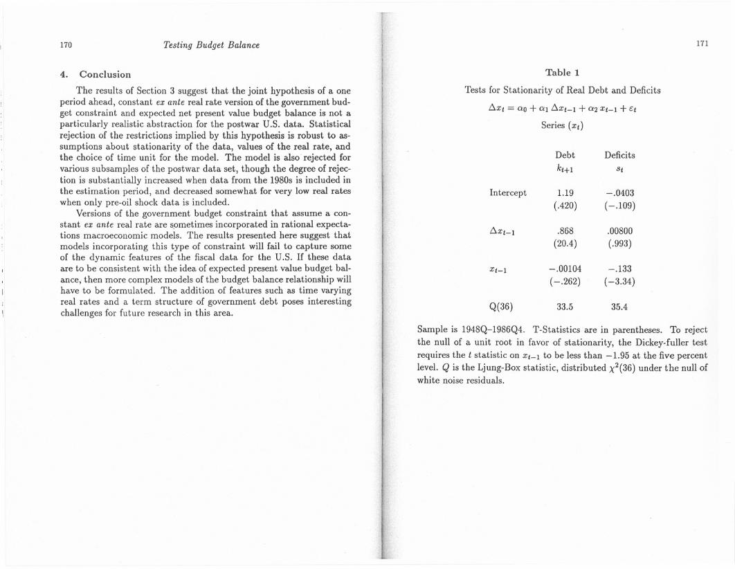
Given that the restrictions imposed by (2.4) require stationarityof St and hence kt, some pretesting for nonstationarity is appropriate.Results of standard Dickey-Fuller (henceforth DF) regressions are givenin Table 1.

Table 1 shows that the Dickey-Fuller test rejects the null of a unitroot for the debt series but not for deficit. These results constitute someprima facie evidence against the validity of the model of Section 2 forpostwar U.S. data. If real debt evolves according to equation (2.4), andreal deficits (surpluses) are stationary, then real debt cannot be non-stationary. Clearly, the budget cannot be balanced in any meaningful"expected present value" sense if debt diverges over time while deficitscontinue to fluctuate in a stationary fashion. On the other hand, it maybe the case that such pessimistic inferences are unwarranted, becauseof biases inherent in the DF test. Sims (1988), Sims and Uhlig (1990),DeJong et al. (1988) and others have questioned the applicability of DFand similar classical procedures for determining the presence of a unitroot. Specifically, many of the results in these papers suggest that theDF test suffers from low power against near-nonstationary alternatives,leading to a bias in favor of the unit root null.

As an alternative to standard DF tests of a unit root, the papersmentioned above employ Bayesian methods to obtain inferences con-

rTesting Budget Balance 167

cerning potential nonstationarity. In Table 2, some of these methods areused to analyze the real debt and deficit series. Following the approachof DeJong and Whiteman (1989 a,b) a sixth order AR model with aconstant term was fit to each series. Assuming a normal likelihoodfunction, and diffuse (normal-gamma) prior for the model parameters,Monte Carlo integration was used to obtain estimates of the posteriormean and standard deviation of the modulus of the largest root of theAR polynomial. These estimates are given in Table 2, along with theapproximate posterior probability that each of the largest roots is insidethe unit circle.

For both series, the Bayesian procedure places most of the posteriorprobability on stationarity. However, the posterior probability of non-stationarity is much higher (about 16%) for debt than for deficits (lessthan .1%). Sims' (1988) test of a unit root as a point null slightly favorsthe unit root over stationarity for debt, and'viCe versa for deficits. Both

. inferences, however, could be reversed by a relatively small change,inprior odds. On balance, the evidence presented in Table 2 suggests thatstationarity is the most likely inference for both series, while difference-stationarity is plausible in the case of debt but somewhat less plausiblefor deficits. Due to this ambiguity concerning the possible presence ofunit roots, two versions of the model were fit to the data. The firstwas the stationary model described in Section 2. The second modelassumes difference-stationarity of the deficit process.

To derive the differenced version of the model, rearrange the termsin equation (2.2) to obtain

00

Skt + St-1 = - L: AT E(Llst+T I Jt-1)T=O

which states that this period's expected deficit including interest pay-ments must be balanced by the discounted sum of expected changesin all future deficits. If {Llst} is taken to be stationary, then equation(3.1) implies that deficits including interest payments, i.e., {Akt} willbe stationary. Now assume that HSR assumptions Al (stationarity)and A2 (nonsingularity) apply to first differences of St. Let the MARfor Llst be given by .

(3.2) St = O"(L)Wt

where 0"is a one-sided lag polynomial and {Wt} is a martingale differ-ence sequence. Applying the Hansen-Sargent (1980a) prediction for-mula to (3.1) yields a unique one sided representation for {Skt+1 +stJ

(3.3) kt+1 = ,.(L)Wt here ,.(z) = [0"(-\)- O"(z)]j(z- -\) .

(3.1)

-10

-20

-30

.4050 55

168 Testing Budget Balance Testing Budget Balance 169

As in the stationary case,equation (3.3)can be directly translated intorestrictions on the MAR of {[(c5kt+l+St),~St]}. Thetermc5kt+l+ Strepresents the current period's expectation of the deficit net of interestat the end of next period, Le., E(~kt+l I Jt-I). Alternatively, thisterm is proportional to kt+I + c5-1st, which represents the discrepancybetween the value of debt and its expected net present value, assuminga constant ex ante real rate and that St follows a random walk. Similarterms appear in the price-dividend/term structure models analyzed byHansenand Sargent (1981e)and Campbell and Shiller (1987),which areformally identical to the difference stationary model analyzed above.

To implement the tests described above, a bivariate vector autore-gression with a constant term was fit to {kt+I, St} for the stationarymodel and {[(c5kt+l + St), ~St]} for the first differences model. Usingmethods described in Campbell and Shiller (1987), the restrictions im-plied by (2,4) and (3.3) were reduced to linear restrictions, and testedby means of likelihood ratio tests.3 Table 3 displays results for bothmodels, under various assumptions about lag lengths and real interestrates.

The results in Table 3 show that the constant ex ante real ratemodel can be rejected at essentially arbitrary significance levels by thepostwar U.S. data. Differencing seems to impact little on the signif-icance level of the test statistics. This strong rejection of the modelstands in sharp contrast to the findings of Hamilton and Flavin (1986),who conclude that equation (2.2) represents a useful approximation forthe postwar U.S. case. Some possible explanations for this discrepancyare considered below.

Hamilton and Flavin's (henceforth HF) study differs from the presentone in the following ways:

1. They use annual (fiscal year) data derived from the unified bud-get series, instead of quarterly data derived from the NIA series.

2. Their sample runs from 1960 through 1984, instead of 1948-1986.

3. They assume that the current surplus net of interest (St) is notGranger caused by debt (kt).

4. As a consequence of (3), they do not formally test the restric-tions implied by equation (2.4). Instead they present evidencethat expected changes in future surpluses account for a sub-stantial amount of the variation in real debt. In particular,they calculate the squared correlation between the real and im-plied debt series to be 0.53.

Of the differences listed above, item (3) represents the most seriousdistinction between the two studies. In assuming that debt does notGranger cause surpluses, HF's approach implies stochastic singula.rityof {(kt+l, St)} and eliminates the possibility of performing tests of crossequa.tion restrictions such as those reported in Table 3. This assump-tion is also strongly rejected by the data: standard tests (not reportedhere) of causality from debt to surpluses reject noncausality at the 1%significance level. In light of these considerations, the assumption ofnoncausality does not appear to be justified by the data.

To provide greater comparibility between my results and those inthe HF study, the application of the levels models tested in Ta.ble 3 wasmodified to more closely resemble that of the HF paper. The data serieswere modified by annualizing the quarterly data (averaging debt andsumming deficits) and restricting the data set to the years 1960-1984.Following HF, a constant ex ante real rate of 1.12 percent was assumed,and a constant term and 3 lags were included in the VAR equations.However, Granger noncausality of surpluses by debt was not assumeddue to considerations mentioned above. The estimation results for this

modified data set are displayed in Table 4. This table show that theresults obtainable with the annualized data set are comparable to thoseobtain~d in the HF study, in the sense that the debt series implied bythe model is highly correlated with the actual debt series. In fact, bydropping the unrealistic assumption that the surplus net of interest isnot caused by debt, sample correlations above .9 can be easily obtained.On the other hand, the cross equation restrictions implied by the modelare still strongly rejected by the modified data. These results do notqualitatively change when the sample period is expanded to the fulldata set (1948-86), or restricted to the years before the enactment ofthe Reagan tax cut (1948-80).

The fact that the model appears to be so consistently and stronglyrejected by the postwar U.S. data led me to experiment with a num-ber of different real interest rates and data subsamples, in order to seewhether the model represents a reasonable approximation for some sub-period of the postwar data set. The best fit was obtained by specifyingthe real rate to be very close to zero and restricting the (annual) dataset to the pre-oil shock period of 1948-73. For this experiment I wasable to obtain X2(7) test statistics of approximately 22. Though thisis still highly significant, applying the Schwarz correction for degreesof freedom yields values for the Schwarz criterion that are only slightlyunfavorable for the restricted model.

170 Testing Budget Balance

4. Conclusion

The results of Section 3 suggest that the joint hypothesis of a oneperiod ahead, constant ex ante real rate version of the government bud-get constraint and expected net present value budget balance is not aparticularly realistic abstraction for the postwar U.S. data. Statisticalrejection of the restrictions implied by this hypothesis is robust to as-sumptions about stationarity of the data, values of the real rate, andthe choice of time uni t for the model. The model is also' rejected forvarious subsamples of the postwar data set, though the degree of rejec-tion is substantially increased when data from the 1980s is included inthe estimation period, and decreased somewhat for very low real rateswhen only pre-oil shock data is included.

Versions of the government budget constraint that assume a con-stant ex ante real rate are spmetimes incorporated in rational expecta-tions macroeconomic models. The results presented here suggest thatmodels incorporating this type of constraint will fail to capture someof the dynamic features of the fiscal data for the U.S. If these dataare to be consistent with the idea of expected present value budget bal-ance, then more complex models of the budget balance relationship willhave to be formulated. The addition of features such as time varyingreal rates and a term structure of government debt poses interestingchallenges for future research in this area.

f 171

Table 1

Tests for Stationarity of Real Debt and Deficits

~Xt = 00 + 01 ~Xt-1 + 02 Xt-1 + C:t

Series (Xt)

Intercept

~Xt-1

Xt-1

Q(36)

Sample is 1948Q-1986Q4. T-Statistics are in parentheses. To reject

the null of a unit root in favor of stationarity, the Dickey-fuller testrequires the t statistic on Xt-1 to be less than-1.95 at the five percentlevel. Q is the Ljung-Box statistic, distributed X2(36) under the null ofwhite noise residuals.

Debt Deficits

kt+1 St

1.19 -.0403

(.420) (-.109)

.868 .00800

(20.4) (.993)

-.00104 -.133

(-.262) (-3.34)

33.5 35.4

172

St

Table 2

Posterior Distribution for Modulus of the LargestAR Root A

Xt = 0'0 +L:~=1O'jXt-l +e

Series (Xt)

Debt

kHl

Deficits

PosteriorMean

.9748 .8654

PosteriorSt. Deviation

.02602 .05748

Pr(A < 1) .8411 .9966

App. Log Oddsin favor of aunit root.

.7978 -.7873Note: Test statistics are distributed X2(2p+ 1) under the null, where pis the number of lags in the VAR model. Original sample is 1948Ql-1986Q4.

Sample is 1949Q3-1986Q4. Calculations are based on 10,000 Monte

Carlo replications. See DeJong and Whiteman (1989a) for a detaileddescription of the Monte Carlo technique.

. Approximate log posterior odds ratio of a unit root versus a stationary

alternative. Following suggestion of Sims (1988), the log of this ratio

is approximated as -log(posterior variance of 11.)-6.5, which assumes4 to 1 prior odds in favor of the stationary alternative.

173

Table 3

Likelihood Ratio Tests of (2.2) and (3.3)

Assumed Constant Ex Ante Real Rate (Annualized)

Lags in r = .2%% r=l% r=2%VAR

Levels Model

4 154 144 1518 165 156 164

Differences Model48 129 129 129

174

Table 4

Tests of Expected NPV Using Annual Data

SamplePeriod

1960-84 1948-86

LikelihoodRatio

[X2(7)]

34.6 76.4

r2 for Actual vs. ImpliedDebt Series

.901 .969

1948-80

40.8

.980

Note: tests assume a constant ex ante real interest rate of 1.12 percent.

f

>.,

-~

Testing Budget Balance 175

Notes

1. Other related papers are Wilcox (1989) and Shim (1984).

2. Inspection of equation (2.1) reveals that (2.1) is a weaker restrictionthan equation (2.1) of HSR. Yet a great deal of confusion exists asto whether it is necessary to assume constant real rates to obtain(2.2). Clearly, only a constant ex ante real rate need be assumed,since (2.2) follows from (2.1).

3. By linearizing the restrictions implied by (2.4), restrictions are ineffect being imposed on the AR rather than the MA representationof the joint process for debt and deficits. Alternatively, imposingrestrictions in this fashion amounts to imposing restrictions usingthe government budget constraint (2.1) instead of the present valuerelation (2.4). Also, the likelihood ratio tests of these restrictionsdepend crucially upon the stationarity of the debt process assumedin the derivation of (2.4). It should 'also be noted that the values ofthe likelihood ratio test statistics are invariant to the (invertible)transformations used to obtain these linear restrictions.

""

a