of “comparable” companies. firm’s own earnings. for” paper.pdfadjusted EBITDA multiples for...

Securities Litigation and Consulting Group, Inc. © 2011.

Rethinking the Comparable Companies Valuation Method1

Abstract: This paper studies a commonly used method of valuing

companies, the comparable companies method, also known as the method

of multiples. We use an intuitive graphical presentation to show why the

comparable companies method is arbitrary and imprecise. We then show

how valuations can be significantly improved using regression analysis.

Regression analysis is superior to the comparable companies method

because, by using more of the available data and imposing fewer

unreasonable assumptions, it is more accurate and can value more firms.

I. Introduction

The valuation of privately-held firms is a substantial and challenging problem.

One method of valuation often used in practice is called the comparable companies

method, also known as the method of multiples. In this method, the value of a firm is

estimated using a handful of “comparable” companies. Some measure of a value-to-

earnings ratio is calculated for each of the comparable companies. To estimate the firm’s

value, one simply multiplies the average of the ratio of the comparable firms by the

firm’s own earnings.

The comparable companies method of valuation is used in many different

contexts. In mergers and acquisitions, analysts on both sides of the transaction often

estimate the value of the target company using this method. It is also used in a variety of

litigation contexts.2 For instance, dissident shareholders may take legal action to dispute

the price proposed for their shares in a merger. Another example occurs when settling

disputes over economic damages and lost profits. The comparable companies method can

be used to estimate the value of the plaintiff’s firm “but-for” an alleged bad act.

1 © 2011 Securities Litigation and Consulting Group, Inc., 3998 Fair Ridge Drive, Suite 250, Fairfax, VA

22033. www.slcg.com. The primary authors are Paul Godek, Craig McCann, Dan Simundza and Carmen

Taveras. Dr. Godek can be reached at 703-246-9382 or [email protected], Dr. McCann can be reached

at 703-246-9381 or [email protected], Dr. Simundza can be reached at 703-539-6779 or

[email protected], and Dr. Taveras can be reached at 703-865-4021 or [email protected]. 2 See Weil, Wagner, and Frank (2001) for a more complete discussion.

http://www.slcg.com/

mailto:[email protected]




2 Rethinking Comparable Companies Method, First Draft.

The comparable companies method is also used when there is a taxable

transaction involving a business. For instance, a business owner might give a family

member shares in a private company as a gift or as an inheritance, and the value of the

business must be estimated to calculate the beneficiary’s gift or estate tax burden. Lastly,

in the context of marital dissolutions, any family businesses must be accurately valued in

order to reach a fair settlement.

In this paper, using real-world data and simple graphs, we examine the

arbitrariness and imprecision of the CCV method and suggest a demonstrably superior

alternative based on regression analysis. Using a simple empirical test we measure the

accuracy of these two valuation methods. We show that the method based on regression

analysis is superior to the comparable companies method because, by using more of the

available data and imposing fewer unreasonable assumptions, it is more accurate and can

value more firms. We value 250 public companies using these two methods and find that

regression analysis generates more accurate predictions for approximately 85% of the

firms. Moreover, we show that regression analysis can accurately value firms which the

comparable companies method cannot.

Our main criticisms of the comparable companies method can be conveyed

through a simple example. Presented with Figure 1, any student in a first-year,

undergraduate statistics course should be able to estimate the relationship between the Y-

variable plotted on the vertical axis and the X-variable plotted on the horizontal axis.

That same student is likely to plot a linear relationship using Ordinary Least Squares that

looks like the solid line in Figure 1 and warn you that, although this is the best she can do

given the data, you should not place much credence in the relationship because you only

gave her six observations. Now, if you instructed her to ignore the observation with the

negative X-value and to assume the relationship between Y and X has to be strictly

proportional, a good student would protest mightily that you now have only five

observations and that Y is clearly not proportional to X and so the resulting relationship

represented by the dashed line is nearly meaningless. In what follows, we explain that

what our first year statistics student knows is worthless passes for analysis under the

comparable companies approach to valuing companies.

Securities Litigation and Consulting Group, Inc. © 2011 . 3

Figure 1: Too Few Observations, Not Enough Freedom

II. Review of the Practitioner-Oriented Comparable Companies

Valuation Literature

The group of comparable companies typically consists of a handful of firms from

the same industry as the firm being valued. The market values of these peer group firms

are known either because they are publicly traded companies or were recently valued in a

market transaction.

The observed market value of the peer group firms used in the numerator of the

ratios can be measured by the market value of their common stock outstanding (equity

value) or by the market value of all their outstanding securities including debt (enterprise

value). The denominator in ratios using equity value is commonly net income or free

cash flow. In ratios using enterprise value, revenue, earnings before interest and taxes

(EBIT) or earnings before interest, taxes, depreciation and amortization (EBITDA) are

common. The comparable companies method implies that equity or enterprise value is a

simple multiple of the measure of earnings, revenues or assets used. Table 1 lists some

valuation multiples commonly referenced in the practitioner-oriented literature.3

3 Sources checked include: Stowe et al (2002), pp. 179-246; Ibbotson Associates (2004), pp. 25-31; Cornell

(1993), pp.56-98; Koller, Goedhart, and Wessels (2010), pp. 287-322; CFA® Program Curriculum (2009),

Volume 3 pp. 269-275; Damodaran (2006), pp. 255-324.

0

20

40

60

80

100

120

140

160

-10 0 10 20 30 40 50 X

Y


Table 1: Commonly Used Multiples

EBITDA

Value Enterprise

EBIT

Value Enterprise

Revenue

Value Enterprise

Assets of ValueBook

ValueEquity

FlowCash Free

ValueEquity

IncomeNet

ValueEquity

Equity multiples can be misleading if there is considerable variation in the amount

of financial leverage across the peer group firms and between the peer group firms and

the firm being valued, as they lead to different valuations for otherwise similar firms.4

Enterprise value multiples are preferable to equity value multiples if there is substantial

variation in financial leverage across the peer group firms and the firm being valued. If

the enterprise value is being estimated, the scaling variable should be a cash flow

available to both equity and debt – EBIT or EBITDA.

After the decision is made to use one or more of the multiples listed in Table 1

and the requisite data is collected, either some of the comparable firms or the target itself

may have a negative or zero-value for the variable in the denominator. For example, the

analyst may decide to value a firm based on enterprise value to EBITDA and equity to

net income ratios for eight publicly traded firms but learn that two of the eight

comparable firms have negative EBITDA and the subject firm has negative net income.

The practitioner literature suggests dropping the two comparable companies with

negative EBITDA values and abandoning the equity to net income multiple. 5

The

standard comparable companies approach thus severely limits the data and methods

available to an analyst resulting in unnecessarily imprecise and inaccurate estimates of

value.

4 For examples, see Koller, Goedhart, and Wessels (2010), p. 307, and Bader (2002), pp. 29-32. These

issues are related to the original insights of Modigliani and Miller that the value of a firm should, as a first

approximation, be independent of its capital structure. See Modigliani and Miller (1958), pp. 261-97, and

Miller (1977), pp. 261-75. 5 For examples see Koller, Goedhart, and Wessels (2010), p. 312, Exhibit 14.6, and Damodaran (2006), p.

260.


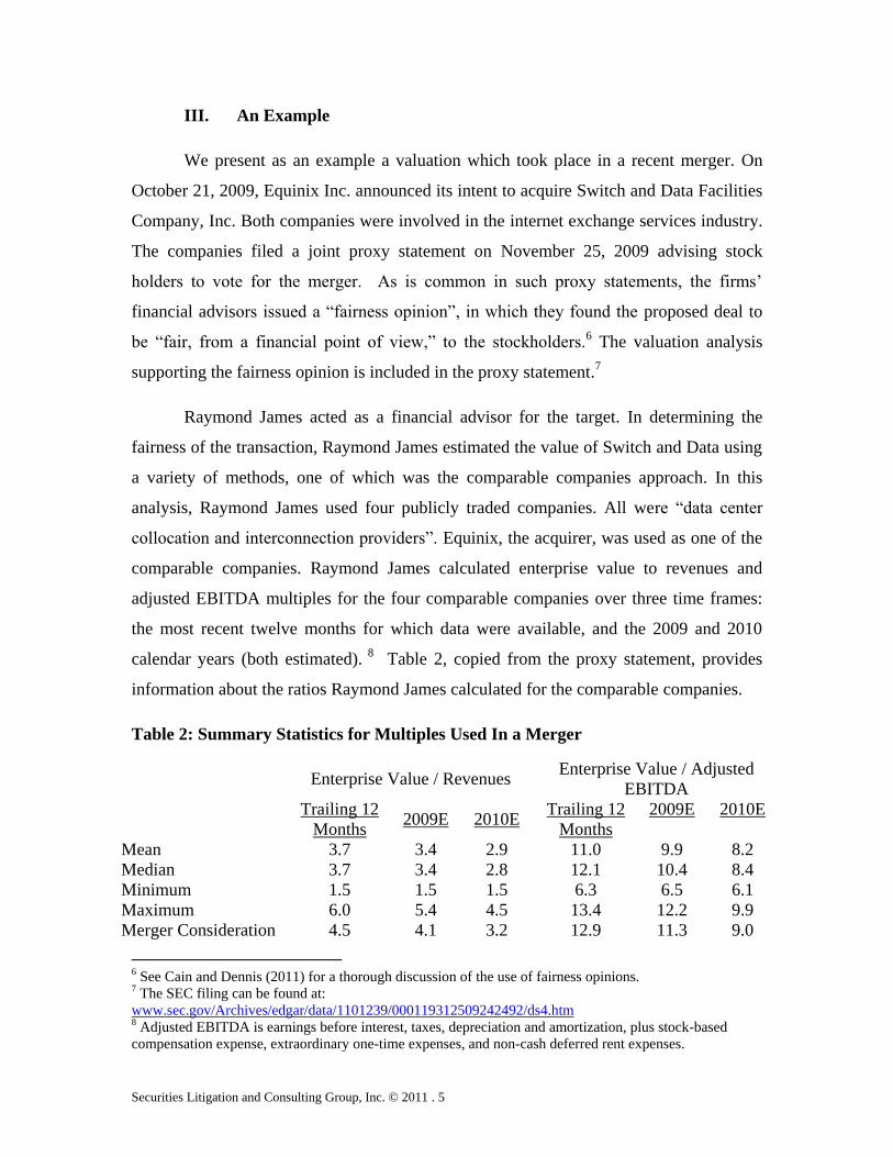
III. An Example

We present as an example a valuation which took place in a recent merger. On

October 21, 2009, Equinix Inc. announced its intent to acquire Switch and Data Facilities

Company, Inc. Both companies were involved in the internet exchange services industry.

The companies filed a joint proxy statement on November 25, 2009 advising stock

holders to vote for the merger. As is common in such proxy statements, the firms’

financial advisors issued a “fairness opinion”, in which they found the proposed deal to

be “fair, from a financial point of view,” to the stockholders.6 The valuation analysis

supporting the fairness opinion is included in the proxy statement.7

Raymond James acted as a financial advisor for the target. In determining the

fairness of the transaction, Raymond James estimated the value of Switch and Data using

a variety of methods, one of which was the comparable companies approach. In this

analysis, Raymond James used four publicly traded companies. All were “data center

collocation and interconnection providers”. Equinix, the acquirer, was used as one of the

comparable companies. Raymond James calculated enterprise value to revenues and

adjusted EBITDA multiples for the four comparable companies over three time frames:

the most recent twelve months for which data were available, and the 2009 and 2010

calendar years (both estimated). 8

Table 2, copied from the proxy statement, provides

information about the ratios Raymond James calculated for the comparable companies.

Table 2: Summary Statistics for Multiples Used In a Merger

Enterprise Value / Revenues

Enterprise Value / Adjusted

EBITDA

Trailing 12

Months 2009E 2010E

Trailing 12

Months

2009E 2010E

Mean 3.7 3.4 2.9 11.0 9.9 8.2

Median 3.7 3.4 2.8 12.1 10.4 8.4

Minimum 1.5 1.5 1.5 6.3 6.5 6.1

Maximum 6.0 5.4 4.5 13.4 12.2 9.9

Merger Consideration 4.5 4.1 3.2 12.9 11.3 9.0

6 See Cain and Dennis (2011) for a thorough discussion of the use of fairness opinions. 7 The SEC filing can be found at:

www.sec.gov/Archives/edgar/data/1101239/000119312509242492/ds4.htm 8 Adjusted EBITDA is earnings before interest, taxes, depreciation and amortization, plus stock-based

compensation expense, extraordinary one-time expenses, and non-cash deferred rent expenses.

http://www.sec.gov/Archives/edgar/data/1101239/000119312509242492/ds4.htm


The first four rows list summary statistics. The last row, titled Merger

Consideration, is included to help interpret these ratios in the context of the merger. The

terms of the merger gave Switch and Data shareholders the choice between 0.19409

shares of Equinix common stock or $19.06 per share for each share of Switch and Data

owned. The values in the last row are the multiples implied by the $19.06 value for shares

of Switch and Data common stock. For instance, the value of 4.5 in the first column of

the last row is found by first computing Switch and Data’s enterprise value under the

hypothesis that each share of common stock is worth $19.06, and then dividing by Switch

and Data’s actual revenue from the previous twelve months. The rest of the values in the

last row are computed in a similar manner.

We can also display the information contained in Table 2 graphically.9 Figure 2

plots enterprise value against revenue over the trailing twelve months for the comparable

companies (i.e. the data in the first column in Table 2).

Figure 2: Enterprise Value and Revenue for the Comparable Companies

9 The proxy statement provides summary statistics of the ratios, but not the underlying data. We used

Bloomberg to access the relevant data. Our multiples are slightly different than those reported in the proxy

statement.

$0

$500

$1,000

$1,500

$2,000

$2,500

$3,000

$3,500

$4,000

$4,500

$5,000

$0 $200 $400 $600 $800 $1,000

En

terp

rise

Va

lue

(Mil

lio

ns)

Revenue (Millions)


To represent the ratio of enterprise value to revenue graphically, we draw a line

from the origin (the 0,0 point on the graph) to each data point on the graph identified with

an X. The slope of a straight line is simply its “rise over run” so the slope of the line

connecting the origin and the company’s data point is equal to the ratio of the firm’s

enterprise value to revenue. These lines have been added to the graph in Figure 3.

Figure 3: Representing Multiples Graphically

The steepest line corresponds to the maximum multiple from Table 1 (6.0), while

the flattest line corresponds to the minimum (1.5). The dark solid line labeled “Average”

represents the mean multiple of the four comparable companies. The graph shows that the

comparable companies are actually quite disparate. This is one reason the CCV method

generates inaccurate predictions.

Using these multiples and estimates of revenue and adjusted EBITDA, Raymond

James computed the implied estimates of the equity price per share of Switch and Data.

These estimates are reported in Table 3.

$0

$500

$1,000

$1,500

$2,000

$2,500

$3,000

$3,500

$4,000

$4,500

$5,000

$0 $200 $400 $600 $800 $1,000

En

terp

rise

Va

lue

(Mil

lio

ns)

Revenue (Millions)


Table 3: Estimates of Switch and Data’s Value of Equity

Enterprise Value / Revenue

Enterprise Value / Adjusted

EBITDA

Trailing

12 Months 2009E 2010E

Trailing

12 Months

2009E 2010E

Mean $14.89 $15.29 $16.55 $15.43 $16.14 $16.88

Median $14.77 $14.90 $15.99 $17.57 $17.29 $17.40

Minimum $2.98 $4.06 $5.82 $6.57 $8.84 $11.35

Maximum $27.02 $27.33 $28.42 $20.00 $21.12 $21.39

Merger

Consideration

$19.06 $19.06 $19.06 $19.06 $19.06 $19.06

To compute the 14.89 value in the first column of the row titled “Mean”, Switch

and Data’s revenue over the previous twelve months is multiplied by the mean multiple

of 3.7, listed in Table 2, to get Switch and Data’s estimated enterprise value of $725

million.10

Subtracting debt, minority interest and preferred shares, and then adding cash,

gives an estimate of Switch and Data’s equity value. Dividing Switch and Data’s equity

value by the number of shares outstanding yields an estimate of the equity value per share

of $14.89.

Figure 4 illustrates this application of the comparable companies approach.

Switch and Data’s estimated enterprise value is the point on the “Average” line directly

above $195.8 million on the revenue axis.11

The range of estimates generated by the

comparable companies approach and reported in Table 3 is quite large and is reflected in

the dispersion of the dotted lines in Figure 2. Using the lowest valuation ratio gives a per

share equity value for Switch and Data of $2.98, while using the largest valuation ratio

gives a per share value of $27.02. Given the number of shares outstanding, this range of

multiple alone could have “justified” a transaction price ranging from $100 to $935

million. To put this range into perspective, the range itself is greater than the actual

transaction price ($670 million).

10 While information on Switch and Data’s revenue over the twelve months prior to the

merger is not publicly available, we estimate it at $195.8 million using data supplied in

the proxy statement. 11 Since we do not have access to the data Raymond James used, our multiple is slightly different than the

value of 3.7 reported in Table 2, and hence our estimated value is slightly lower.


Figure 4: Estimated Enterprise Value

IV. Methodology

In this section, we describe a simple test of the accuracy of the comparable

companies approach to valuation. We use Bloomberg to obtain financial data for 250

public firms in the three Standard Industry Classification (SIC) codes described in Table

4. We will value each of these firms, using other firms in the same industry as its

comparables, and compare the accuracy of the different methods.

Our analysis will use two multiples: Enterprise-Value-to-EBITDA, and

Enterprise-Value-to-Revenue. Enterprise value is calculated as of December 31, 2010.

EBITDA and Revenue are measured over the 2010 calendar year. Since fiscal years can

vary by firm, we collected quarterly data and aggregated the EBITDA and revenue data

so that all firms are measured over the same time period.12

We discarded 19 firms whose

fiscal quarters do not align with the calendar quarters.

We define two samples for each multiple: the firms with positive multiples (the

“Positive” sample), and all firms (the “Full Dataset” sample). The comparable companies

12 Because of earnings revisions and corrections, the sum of the quarterly measures does not always equal

the annual measures. Due to the firms’ different fiscal years, it is not possible to use the updated annual

measures for all firms. Our qualitative results do not change when using revised annual earnings where

possible (i.e. the firms whose fiscal year ends on 12/31/2010.)

$0

$500

$1,000

$1,500

$2,000

$2,500

$3,000

$3,500

$4,000

$4,500

$5,000

$0 $200 $400 $600 $800 $1,000

En

terp

rise

Va

lue

(Mil

lio

ns)

Revenue (Millions)


method is only used on the Positive sample, while the regression method is used on both

samples. Table 4 provides information about the different samples we use by industry.

Table 4: Description of Industries and Samples

EV/EBITDA EV/Revenue

Positive

Sample

Full Dataset

Sample

Positive

Sample

Full Dataset

Sample

Pharmaceutical Preps (2834) 72 219 185 229

Perfumes & Cosmetics (2844) 7 11 12 12

Household Audio & Video (3651) 6 8 9 9

While all of firms within the same SIC code are in the same industry, they may

nevertheless not be truly “comparable”. For instance, in the pharmaceutical industry,

long-established, multi-billion dollar firms like Pfizer and Johnson & Johnson should not

be used to value young, small firms who have little revenue and who derive most of their

value from potential future success. Therefore, in the Pharmaceutical industry, we limit

the group of comparable firms to be those with similar enterprise values to the firm being

valued. The results we present below use the next 10 larger firms, and the next 10 smaller

firms (for a total of 20), as the group of comparable companies.13

The Comparable Companies Method

The comparable companies estimates are computed in the same manner as

described earlier in this paper. For each firm in the sample, we compute the Enterprise-

Value-to-EBITDA and Enterprise-Value-to-Revenue ratios for the comparable

companies, average these ratios, and multiply the average peer company ratio by either

the subject firm’s EBITDA or Revenue .

The Regression Method

The original motivation for this paper came from an observation that the

comparable companies method is in fact quite similar to running a regression on an

extremely small sample of comparable firms, with the regression constant constrained to

equal zero. Since there is no compelling reason that enterprise value must be directly

13 We experimented with different size groups and found no substantive change in the qualitative results.


proportional to EBITDA or Revenue, we relax this constraint in our regression analysis.

We model enterprise value as a linear function of the earnings variable:

where is enterprise value, is either EBITDA or Revenue, α and β are parameters

to be estimated, and ε is the error term. We follow Liu, Nissim, and Thomas (2002) and

scale both sides by enterprise value. This is done to correct for Heteroskedasticity, and, as

explained in Baker and Ruback (1999), is likely to give more precise estimates. The

equation we estimate is:

. We estimate this equation using

ordinary least squares, which chooses values for α and β that minimize the sum of the

squared differences between the actual and predicted enterprise values. The group of

comparable firms is formed in the same way as in the comparable companies estimates.

The estimate of enterprise value is computed as where

is the

target firm’s predicted enterprise value, is the value of the target’s scaling variable,

is the estimate of the constant, and is the estimate of the slope coefficient.14,15

Comparing the Comparable Companies and Regression Methods

To measure accuracy, we compute the absolute percentage error of each estimate.

The absolute percentage error is defined as the absolute value of the difference between

the estimated value and the true value, divided by the true value.

Before stating our results, it is useful to see how the two estimation techniques

differ graphically. We will show how the comparable companies and regression analysis

methods estimate the value of Astex Pharmaceuticals, Inc. For expository purposes, the

group of comparable companies is limited to five firms of similar value from the same

SIC code (2834). This example was chosen from our dataset because it nicely illustrates

the problems with the comparable companies method and shows how the regression

method can improve the valuation. Figure 5 plots enterprise value and EBITDA for the

five comparable companies.

14 A similar model omitting the constant was also estimated. As expected, this model, which effectively

restricts the constant to be zero, performed worse than the unconstrained model. 15Extending the model to incorporate more than one measure of earnings as an explanatory variable does

not improve estimates. The problem is that the earnings variables are highly correlated, which leads to

“multicollinearity” in the explanatory variables. As explained in Greene (2003), the variance of the

estimated slope coefficients becomes very large when the explanatory variables are highly correlated.

When this is the case, the predicted values become very inaccurate.


Figure 5: Enterprise Value and EBITDA for the Comparable Companies

The enterprise-value-to-EBITDA multiples for these five firms can be represented

graphically by drawing a line from the origin to the data point for each firm. These

multiples, along with the average, are shown in Figure 6.

Figure 6: Representing Multiples Graphically

$0

$20

$40

$60

$80

$100

$120

$140

$160

$0 $5 $10 $15 $20 $25 $30 $35 $40 $45

En

terp

rise

Va

lue

(Mil

lio

ns)

EBITDA (Millions)

$0

$20

$40

$60

$80

$100

$120

$140

$160

$0 $5 $10 $15 $20 $25 $30 $35 $40 $45

En

terp

rise

Va

lue

(Mil

lio

ns)

EBITDA (Millions)


Astex’s approximately $110 million estimated enterprise value, computed by

multiplying the mean of the comparable companies’ multiples by the Astex’s $16.4

million EBITDA, is illustrated in Figure 7.

Figure 7: Graphical Representation of the CCV Estimate

Some of the practitioner-oriented literature suggests using the median of the

multiples in addition to, and sometimes instead of, the mean. To use the median multiple

graphically, we would simply use the firm with the median slope to predict the target’s

value instead of drawing a new line with the average (mean) slope.

In Figure 8 we plot the predicted enterprise value against the observed enterprise

value. The prediction error is the vertical distance between the two points. In order to turn

this into a percentage error, we would simply divide the prediction error by the observed

enterprise value of the firm. In this case, the predicted value is $108.8 million, while the

observed enterprise value of Astex Pharmaceuticals is $42.9 million. This corresponds to

a percentage error of more than 150%. If we use the median multiple, the estimated

enterprise value is $105.2 million, giving a percentage error of 145.3%.

$0

$20

$40

$60

$80

$100

$120

$140

$160

$0 $5 $10 $15 $20 $25 $30 $35 $40 $45

En

terp

rise

Va

lue

(Mil

lio

ns)

EBITDA (Millions)


Figure 8: CCV Prediction Error

Regression analysis, on the other hand, fits a line to the data in order to minimize

the sum of the squared prediction errors. The prediction line for the regression for the

valuation of Astex is shown in Figure 9. To compute the estimated value, we multiply

Astex’s $16.4 million EBITDA by the estimated 1.19 slope coefficient and add the

estimated 44.25 constant. The predicted value and error are also shown in Figure 9.

Figure 9: Regression Analysis Predicted Values and Prediction Error

Predicted Value

Observed Value

Pre

dic

tion E

rror

$0

$20

$40

$60

$80

$100

$120

$140

$160

$0 $5 $10 $15 $20 $25 $30 $35 $40 $45

En

terp

rise

Va

lue

(Mil

lio

ns)

EBITDA (Millions)

Predicted Value

Observed Value

$0

$20

$40

$60

$80

$100

$120

$140

$160

$0 $10 $20 $30 $40 $50

En

terp

rise

Va

lue

(Mil

lio

ns)

EBITDA (Millions)


The estimate obtained from regression analysis is $63.8 million, which

corresponds to a prediction error of 48.7%. This is much lower than the comparable

companies estimates percentage error of over 150%.

V. Results

In this section we present the results of our empirical analysis. There are three

ways in which regression analysis is superior to the comparable companies method. First,

regression analysis is more accurate when it is constrained to use the same data as the

comparable companies method. Second, it is able to take advantage of more data than the

comparable companies method, and its estimates improve when using this data. Third,

regression analysis can value firms which the comparable companies method cannot.

Table 5 provides summary statistics of the absolute percentage errors obtained

from our different estimation methods. Three estimation techniques are used in this table:

the comparable companies method with both the mean and median multiple, and

regression analysis. All valuations in this table are on firms from the Positive sample,

using only firms from the Positive sample as comparables. The table is split into two

parts because results are reported when both EBITDA and revenue are used as

explanatory variables.

Table 5: Absolute Percentage Errors of Comparable Companies and Regression

Estimates

EBITDA as the Explanatory Variable

Estimation Method Absolute Percentage Error

Mean Median

CCV – Mean 389.3% 107.0%

CCV – Median 102.1% 64.3%

Regression 55.5% 39.7%

Revenue as the Explanatory Variable

Estimation Method Absolute Percentage Error

Mean Median

CCV – Mean 11,641.8% 1,016.4%

CCV – Median 11,217.7% 957.5%

Regression 31.7% 9.0%


The first two rows of Table 5 show that the median multiple performs much

better than the mean multiple as an estimator in the comparable companies method. This

is because the mean can easily be skewed by one or two large values, while the median is

less susceptible to this problem.

The third row in Table 5 reports the results of the regression analysis estimates.

Comparing this row to the first two rows in the table provides a direct comparison of the

comparable companies and regression analysis methods of valuation. The same firms are

valued, using the same group of comparables, for each method. The mean and median

absolute percentage errors are smallest when using the regression analysis method. This

shows that the regression method generates, on average, more accurate estimates than the

comparable companies method. As further evidence, we found that the estimate from

regression analysis was better than the comparable companies estimate for more than

84% of the firms.

The regression estimates are much better because the regression technique does

not impose as many restrictions on the data as the comparable companies method. In

particular, value need not be directly proportional to the scaling variable in the regression

model. While the comparable companies method effectively imposes this constraint, the

regression method does not. In addition, the Ordinary Least Squares algorithm chooses

the parameters to minimize the sum of squared errors in the group of comparables. The

comparable companies method, in contrast, simply uses the mean or median of the

comparable firms’ ratios. This renders the comparable companies estimates more

susceptible to outliers.

Another advantage of the regression analysis method of valuation is that it can

make use of more data than the comparable companies method. Returning to our earlier

example of valuing Astex Pharmaceuticals, Figure 10 shows why the comparable

companies method does not typically include firms with negative multiples in its

analysis.


Figure 10: The Comparable Companies with Negative Multiples

This graph is identical to Figure 4 except a firm with negative EBITDA has been

added to the group of comparable companies. The two firms with EBITDA near zero in

the graph provide approximately the same information: in particular, firms can have a

positive enterprise value even with very low EBITDA. The comparable companies

method would typically discard the observation on the firm with the negative EBITDA.

This is because its multiple would be a very large negative number. In contrast, the

“nearby” firm with the slightly larger (and positive) EBITDA would have a very large

positive multiple. So even though these firms provide very similar information, the

comparable companies method would treat them very differently.

Regression analysis, on the other hand, can easily incorporate this additional

observation. If the firms are otherwise comparable, it is wasteful to throw out useful

information. The regression method therefore allows the analyst to take advantage of

more data than the comparable companies method. Figure 11 shows how the predicted

values of the regression change as the additional observation is taken into account.

$0

$20

$40

$60

$80

$100

$120

$140

$160

-$10 $0 $10 $20 $30 $40 $50

En

terp

rise

Va

lue

(Mil

lio

ns)

EBITDA (Millions)


Figure 11: Regression Analysis Predicted Values with Negative Multiples

The solid line is the original prediction line, estimated without the firm with

negative EBITDA. The dashed line is the new prediction line after taking into account all

relevant data. In this case, the predicted value of Astex, which has an EBITDA of $16.4

million, decreases, and the estimate moves closer to the true value.

The summary statistics in Table 6 show that the valuation can be improved by

incorporating all available information.

Table 6: Absolute Percentage Errors When Including All Information

EBITDA as the Explanatory Variable

Estimation Method Sample

Valued

Comparables

Sample Absolute Percentage Error

Mean Median

Regression Positive Positive 55.5% 39.7%

Regression Positive Full Dataset 27.3% 10.7%

Regression Full Dataset Full Dataset 50.8% 7.4%

Revenue as the Explanatory Variable

Estimation Method Sample

Valued

Comparables

Sample Absolute Percentage Error

Mean Median

$0

$20

$40

$60

$80

$100

$120

$140

$160

-$5 $5 $15 $25 $35 $45

En

terp

rise

Va

lue

(Mil

lio

ns)

EBITDA (Millions)


Regression Positive Positive 31.7% 9.0%

Regression Positive Full Dataset 31.3% 7.1%

Regression Full Dataset Full Dataset 32.4% 7.4%

The third row of Table 5 is reproduced here as the first row of Table 6 for ease

of comparison. Comparing the first two rows in Table 6 shows that valuation accuracy

improves when more information is included in the estimation process. The sample of

firms being valued is the same for these two rows (the Positive sample). The difference

between these rows is in which firms are included in the group of comparable companies:

in the second row, the comparable firms might have negative earnings, while in the first

row all comparable firms must have positive earnings.16

Since the average absolute

percentage errors are smaller in the second row of Table 6, using all available data

improves the valuation’s accuracy.

The estimates in the third row of Table 6 come from valuing all of the firms in

our database, including those with negative earnings variables. The mean and median

absolute percentage errors are approximately equal to the corresponding values in the

second row, and do not differ in any systematic way. The regression method can be used

to accurately value firms which the comparable companies method cannot.

These results show that the regression analysis method of valuation is superior

to the comparable companies method for three reasons. First, regression analysis is more

accurate when it is constrained to use the same data as the comparable companies

method. Second, it is able to take advantage of more data than the comparable companies

method, and its estimates improve when this data is used. Third, it is able to accurately

value firms which the comparable companies method cannot.

VI. Conclusion

This paper studied the Comparable Companies Valuation method as it is

commonly used in practice. We presented a simple graphical description of the algorithm

underlying the comparable companies method. These graphs show intuitively why the

16 In the context of our graphical analysis the group of comparables for estimations in the second row might

look like Figure 10, while the group of comparables for estimations in the first row must look like Figure 5.


this method generates poor predictions of value. It is a very rudimentary technique

without rigorous foundation.

We then showed that an alternative prediction methodology using regression

analysis performs much better than the comparable companies method. The estimates

using regression analysis were shown to be much closer to the true value when using the

same set of information as the comparable companies method. Additionally, regression

analysis is able to take advantage of useful information contained in observations on

firms with negative multiples. Including this information in the sample improves the

estimates. Since the computational cost of using regression analysis is only slightly

higher than the comparable companies method, we argue that practitioners should forego

the comparable companies method in favor of using regression analysis.

References

Bader, L., “Valuing Companies, Valuing Pension Plans,” Contingencies,

September/October 2002.

Baker, M. and Rubak R. S., “Estimating Industry Multiples,” Working Paper, 1999.

Cain, M. and Dennis, D., “Information Production by Investment Banks: Evidence From

Fairness Opinions,” Working Paper, 2011.

CFA® Program Curriculum, Corporate Finance Level II, Pearson Custom Publishing,

Boston, 2009.

Cornell, B., Corporate Valuation, Irwin, 1993.

Damodaran, A., Damodaran on Valuation: Security Analysis for Investment and

Corporate Finance, Second Edition, Wiley Finance, 2006.

Greene, W., Econometric Analysis, Fifth Edition, Prentice Hall, 2003.

Ibbotson Associates, Cost of Capital 2004 Yearbook, Ibbotson Associates, Chicago,

2004.

Koller, T., Goedhart, M., and Wessels, D., Valuation: Measuring and Managing the

Value of Companies, McKinsey & Company, 5th Edition, John Wiley and Sons, 2010.

Liu, J., Nissim D., and Thomas, J., “Equity Valuation Using Multiples,” Journal of

Accounting Research, Vol. 40, No. 1, 2002.


Miller, M.H., “Debt and Taxes,” Journal of Finance, Vol. 32, No. 2, May, 1977.

Modigliani, F., and Miller, M.H., “The Cost of Capital, Corporation Finance and the

Theory of Investment,” American Economic Review, June 1958.

Stowe, J., Robinson T., Pinto, J, and McLeavey, D. Analysis of Equity Investments:

Valuation, Association for Investment Management and Research, 2002.

Weil, R., Wagner, M., and Frank, P. Litigation Services Handbook: The Role of the

Financial Expert, Third Edition, John Wiley & Sons, 2001.

of “comparable” companies. firm’s own earnings. for” paper.pdfadjusted EBITDA multiples for...

Documents

Transcript of of “comparable” companies. firm’s own earnings. for” paper.pdfadjusted EBITDA multiples for...