OF A GRAPHICS BASED TWO-ATTEIBUTE … 276 DEVELOPMENT OF A GRAPHICS BASED TWO-ATTEIBUTE UTILITY 1/3...

0-RIO? 276 DEVELOPMENT OF A GRAPHICS BASED TWO-ATTEIBUTE UTILITY 1/3ASSESSMENT PROGRAM W..(U) AIR FORCE INST OF TECHWRIGHT-PRTTERSON AF9 OH E H MANNER DEC 96

LNCLRSSIFIED AFIT/CI/NR-87--flTF/O 12/4 NL

mEohhhmhohhhEEEhElhEmhEmhEEE

-r 1.0 - ~

"2th~iU. L3,.E2

AU

- e- w w a a .. w a - a a w a ~ wU&

iNC -ASS 11- 11ECURITY CLASSIFICATION OF THIS PAGE (W1hon Dae. 1Entered), 9'

REPORT DOCUMENTATION PAGE READ__________________

*REPORT NUMBER 2. GOVT ACCESSION NO. 3. RECIPIENT'S CATALOG NUMBER

cAFIT/CI/NR 87- 73T /4. TITLE (and Subtitle) 5. TYPE OF REPORT 6 PERIOD COVERED

Development Of A Graphics Based Two-Attribute THESIS/i~UY~XNNUtility Assessment Program With Application 6. PERFORMING 014G. REPORT NUMBERTo Mission Planning

'AUTHOR(&) B. CONTRACT OR GRANT NUMBER(&)

(0 Eleonore H. Wanner

PERFORMING ORGANIZATION NAME AND ADDRESS 10. PROGRAM ELEMENT. PrOJECT, TASK

I% Rensselaer Polytechnic Institute00_ I. CONTROLLING OFFICE NAME AND ADDRESS 12.cemb0erT DAT

AFIT/NR 183mt- 18WPAFB Oil 45433-6583 I3. NUMBER OF PAGES

14. MONITORING AGENCY NAME & AOORESSI different fromt Conutrolling Office) 15. SECURITY CLASS. (of thin report)

UNCLASSIFIEDISs. DECLASSIFICATION. DOWNGRADING

SCHEDULE

IS. DISTRIBUTION STATEMENT (of this Report)

APPROVED FOR PUBLIC RELEASE; DISTRIBUTION UNLIMITED D T IC

IS. SUPPLEMENTARY NOTES W

APPROVED FOR PUBLIC RELEASE: lAW AFR 190-1 417Dean for Research a!

Professional DevelolpmentAFIT/NR

19. KEY WORDS (Continue on reverse side It neceary end Identify by block number)

20. AB3STRACT (Continue on reverse side It necessary and identify by block number)

ATTACH ED.1

DD I JA 7 1473 EDITION OF I NOV 65 IS OBSOLETE

SECURITY CLASSIFICATION OF THIS PAGE ("oun Date Entered)

9-7.0 4wO /6

3

DEVELOPMENT OF A GRAPHICS BASED TWO-ATTRIBUTE UTILITYASSESSMENT PROGRAM

WITH APPLICATION TO MISSION PLANNING

by

Eleonore H. Wanner

A Project Submitted to the Graduate

Faculty of Rensselaer Polytechnic Institute

in Partial Fulfillment of the

Requirements for the Degree of

MASTER OF SCIENCE

r 6r

F). t

Approved: New Y

Dr. James M. TienThesis Advisor

Rensselaer Polytechnic InstituteTroy, New York

December 1986

~Na

CONTENTS

Page

LIST OF FIGURES ........................................... iv

FOREWORD .................................................. ix

ABSTRACT ................................................... x

1. INTRODUCTION ........................................... 1

2. MULTI-ATTRIBUTE UTILITY THEORY ......................... 4

2.1 Terminology and Assumptions ........................ 42.2 Utility Assessment Methods ......................... 7

2.2.1 Ranking Methods ............................ 82.2.2 Category Methods ........................... 92.2.3 Direct Methods ............................. 92.2.4 Indifference Methods ........................ 92.2.5 Gamble Methods ............................ 10

2.3 Utility Independence Properties .................. 13

2.3.1 Mutual Utility Independence ............... 142.3.2 Additive Independence ...................... 152.3.3 Utility Independence in One Direction ..... 162.3.4 No Utility Independence ................... 16

2.4 Utility Function Determination .................... 17

2.4.1 Curve Fitting Approach .................... 172.4.2 Pre-Specified Form ......................... 18

3. A TWO-ATTRIBUTE UTILITY GRAPHICS PROGRAM .............. 22

3.1 Software and Hardware Specifications ............. 223.2 Example Session .................................. 23

3.2.1 Additive and Mutual UtilityIndependence .............................. 23

3.2.2 Utility Independence in One Direction ..... 543.2.3 No Utility Independence ................... 54

4. APPLICATION TO MISSION PLANNING ........................ 69

4.1 Problem Discussion ............................... 694.2 Five Step Assessment Procedure ................... 70

ii

4.2.1 Introduce Terminology and Ideas............ 704.2.2 Utility Assessment for Mission

Planner 1.................................... 71

4.2.3 Utility Assessment for MissionPlanner 2................................... 95

4.2.4 Comments and Critiques..................... 138

5. CONCLUSIONS............................................ 139

5.1 Extensions and Areas for Further Research ........1395.2 Concluding Remarks................................ 140

REFERENCES............................................. 142

APPENDIX Program Listing............................. 143

LIST OF FIGURES

Page

Figure 2.1 General Equations for Common Utility Curves.. .21

Figure 3.1 Program Introduction .......................... 24

Figure 3.2 Attribute Information ......................... 25

Figure 3.3 Lottery Directions ............................ 26

Figure 3.4 Lottery for Time at Moneymax .................. 27

Figure 3.5 Lottery for Money at Timemax .................. 28

Figure 3.6 Possible Inconsistency Indicated .............. 30

Figure 3.7 Previous Responses for Time C.E.'s ............ 31

Figure 3.8 Lottery Specifying Mutual UtilityIndependence .................................. 32

Figure 3.9 Lottery Specifying Additive Independence ...... 33

Figure 3.10 Mutual Utility Independence Indicated ......... 14

Figure 3.11 Additive Independence Indicated ............... 35

Figure 3.12 C.E. for Time Marginal Utility CurveDetermination ................................. 37

Figure 3.13 C.E. for Money Marginal Utility CurveDetermination ................................ 38

Figure 3.14 Program Inability to Assess Utility ........... 39

Figure 3.15 Finding Scaling Relationship .................. 41

Figure 3.16 Indifference Point Selection .................. 43

Figure 3.17 Representation of Viewpoints .................. 44

Figure 3.18 Viewpoints Offered ............................ 45

Figure 3.19 Viewpoint 1 (Example Session) ................. 46




iv

Figure 3.23 Viewpoint 5 (Example Session).................50




Figure 3.27 Utility Independence One Way Indicated ........ 55

Figure 3.28 C.E. for Money Marginal Utility CurveDetermination ................................. 56

Figure 3.29 C.E. for Time Marginal Utility CurveDetermination (at Moneysin) ................... 57

Figure 3.30 C.F. for Time Marginal Utility CurveDetermination (at Moneymax) .................... 58

Figure 3.31 No Utility Independence Indicated ............. 59

Figure 3.32 Decomposition of Ranges Chosen ................ 61

Figure 3.33 Direct Assessment Chosen ....................... 62

Figure 3.34 Direct Assessment Points 1-6 .................. 63

Figure 3.35 Direct Assessment Points 7-12 ................. 64

Figure 3.36 Direct Assessment Points 13-18 ................ 65




Figure 4.1 Attribute Information ......................... 72

Figure 4.2 Lottery for Pa at Pdain (MP 1) ................ 73

Figure 4.3 Lottery for Pa at Pd.so (MP 1) ................ 74

Figure 4.4 Lottery for Pd at Pamax (MP 1) ................ 75

Figure 4.5 Lottery for Pa at Pd.25 (MP 1) ................ 76

Figure 4.6 Lottery for Pd at Pa.so (MP 1) ................ 77

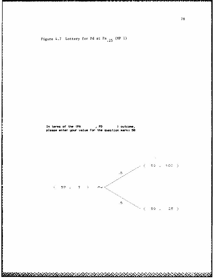
Figure 4.7 Lottery for Pd at Pa.25 (MP 1) ................ 78

V

Figure 4.8 Lottery for Pa at Pdmax (MP 1) ................ 79

Figure 4.9 Lottery for Pd at Pasin (MP 1) ................ 80

Figure 4.10 Lottery for Pa at Pd.75 (MP 1) ................ 81

Figure 4.11 Lottery for Pd at Pa.7s (MP 1) ................ 82

Figure 4.12 Utility Independence One Way Indicated(MP 1) ........................................ 83

Figure 4.13 C.E. for Pd Marginal Utility CurveDetermination (MP 1) .......................... 84

Figure 4.14 C.E. for Pa Marginal Utility CurveDetermination (at Pd.in) (MP 1) ............... 85

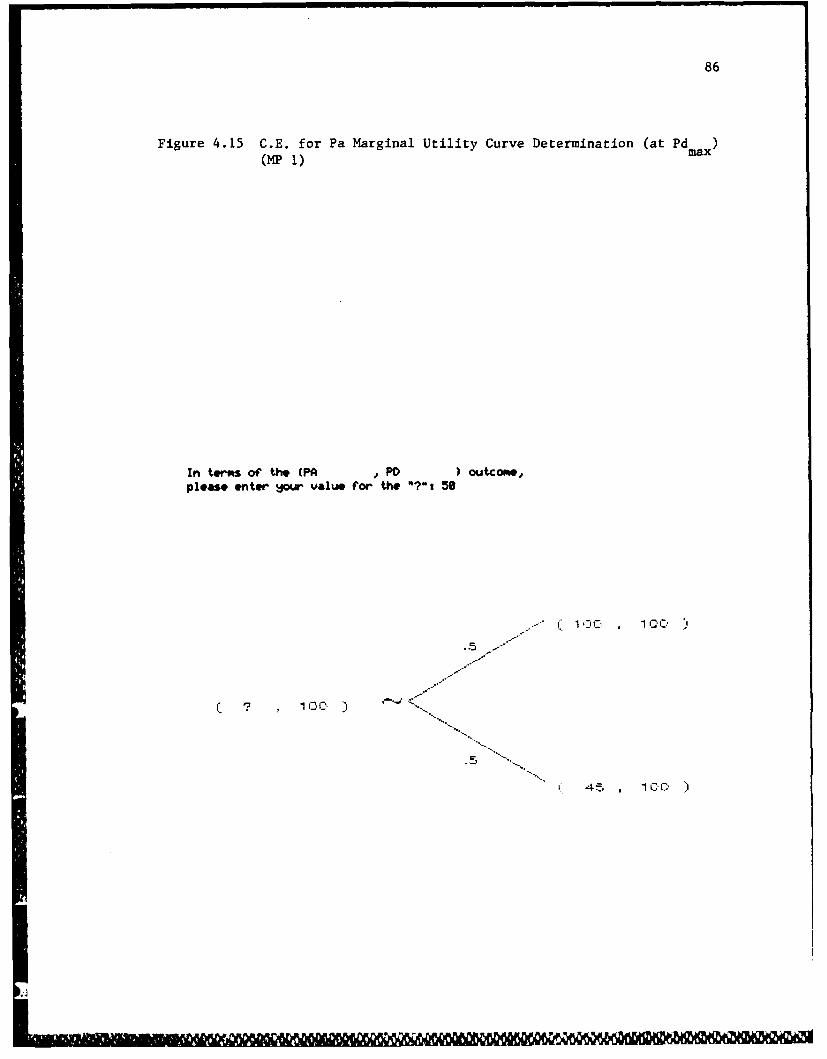
Figure 4.15 C.E. for Pa Marginal Utility CurveDetermination (at Pdsax) (MP 1) ............... 86

Figure 4.16 Viewpoint 1 (MP 1) ............................ 87








Figure 4.24 Attribute Information (lst try, MP 2) ......... 96

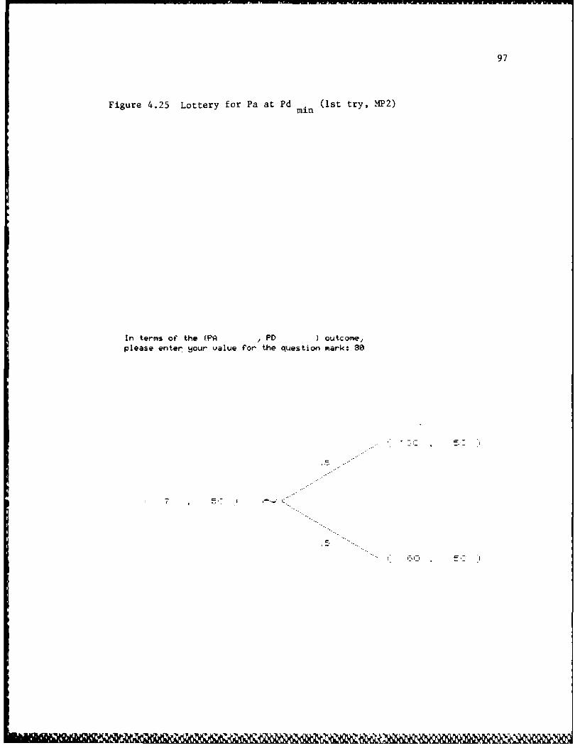
Figure 4.25 Lottery for Pa at Pdlin (lat try, MP 2) ....... 97

Figure 4.26 Lottery for Pa at Pd.5o (lst try, MP 2) ....... 98

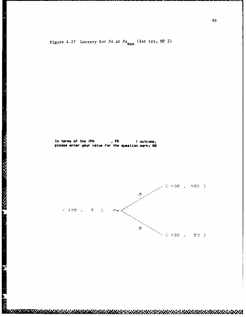
Figure 4.27 Lottery for Pd at Pamax (list try, MP 2) ....... 99

Figure 4.28 Lottery for Pa at Pd.25 (lat try, MP 2) ...... 100

Figure 4.29 Lottery for Pd at Pa so (lIst try, MP 2) ...... 101

Figure 4.30 Lottery for Pd at Pa.2s (lIt try, MP 2) ...... 102

Figure 4.31 Lottery for Pa at Pdsax (lat try, MP 2) ...... 103

vi I

Figure 4.32 Lottery for Pd at Paman (1st try, MP 2) .......104

Figure 4.33 Lottery for Pa at Pd.75 (1st try, MP 2) ...... 105

Figure 4.34 Lottery for Pd at Pa.75 (lst try, MP 2) ...... 106

Figure 4.35 Possible Inconsistency Indicated(1st try, MP 2) .............................. 107

Figure 4.36 Previous Responses for Pd C.E.'s(1st try, MP 2) .............................. 108

Figure 4.37 No Utility Independence Indicated(1st try, MP 2) .............................. 109

Figure 4.38 Decomposition of Ranges Chosen(Ist try, MP 2) .............................. 110

Figure 4.39 Previous Responses for Pa C.E.'s(1st try, MP 2) .............................. 111

Figure 4.40 Previous Responses for Pd C.E.'s(Ist try, MP 2) .............................. 112

Figure 4.41 Decomposition of Ranges Rechosen(1st try, MP 2) .............................. 113

Figure 4.42 Attribute Information (2nd try, MP 2) ........ 115

Figure 4.43 Lottery for Pa at Pdmin (2nd try, MP 2) ...... 116

Figure 4.44 Lottery for Pa at Pd.so (2nd try, MP 2) ...... 117

Figure 4.45 Lottery for Pd at Pamax (2nd try, MP 2) ...... 118

Figure 4.46 Lottery for Pa at Pd.2s (2nd try, MP 2) ...... 119

Figure 4.47 Lottery for Pd at Pa.so (2nd try, MP 2) ...... 120

Figure 4.48 Lottery for Pd at Pa.2s (2nd try, MP 2) ...... 121

Figure 4.49 Lottery for Pa at Pdmax (2nd try, MP 2) ...... 122

Figure 4.50 Lottery for Pd at Pamin (2nd try, MP 2) ...... 123

Figure 4.51 Lottery for Pa at Pd.7s (2nd try, MP 2) ...... 124

Figure 4.52 Lottery for Pd at Pa.7s (2nd try, MP 2) ...... 125

Figure 4.53 Utility Independence One Way Indicated(2nd try, MP 2) .............................. 126

vii

Figure 4.54 C.E. for Pd Marginal Utility Curve Determi-

nation (at Pasin) (2nd try, MP 2) ............ 127

Figure 4.55 C.E. for Pa Marginal Utility .CurveDetermination (2nd try, MP 2) ................ 128

Figure 4.56 C.E. for Pd Marginal Utility Curve Determi-nation (at Pasax) (2nd try, MP 2) ............ 129

Figure 4.57 Viewpoint 1 (MP 2) ........................... 130


Figure 4.59 Viewpoint 3 (NP 2) ........................... 132




Figure 4.63 Viewpoint 7 (Mi 2) ........................... 136


vii-i

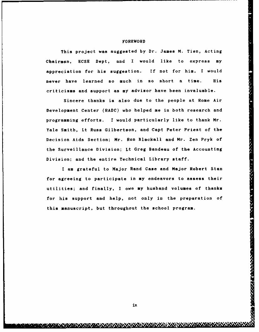
FOREWORD

This project was suggested by Dr. James M. Tien, Acting

Chairman, ECSE Dept, and I would like to express my

appreciation for his suggestion. If not for him, I would

never have learned so much in so short a time. His

criticisms and support as my advisor have been invaluable.

Sincere thanks is also due to the people at Rome Air

Development Center (RADC) who helped me in both research and

programming efforts. I would particularly like to thank Mr.

Yale Smith, Lt Russ Gilbertson, and Capt Peter Priest of the

Decision Aids Section; Mr. Ron Blackall and Mr. Zen Pryk of

the Surveillance Division; Lt Greg Bandeau of the Accounting

Division; and the entire Technical Library staff.

I am grateful to Major Rand Case and Major Robert Stan

for agreeing to participate in my endeavors to assess their

utilities; and finally, I owe my husband volumes of thanks

for his support and help, not only in the preparation of

this manuscript, but throughout the school program.

ixI

v ABSTRACT

A multi-attribute utility assessment-program is

developed which can handle consequences composed of two

attributes. It handles four particular cases of utility

independence properties: additive independence, mutual

utility independence, utility independence in one direction,

and no independence properties. A two-attribute consequence

space was chosen particularly for the ability to represent

the. multi-attribute utility function graphically in three

dimensions, from one of eight possible viewpoints. The

utilities of two Air Force mission planners were assessed to

determine the feasibility of using probability of arrival

and probability of target destruction as factors for mission

success. Based on the results, it appears as though multi-

attribute utility theory would be a definite help to Air

Force mission planning.

887 10 20 16

1

1. INTRODUCTION

Utility theory is a relatively new methodology for

decision making. Relatively new, that is, when compared to

probability theory from which it gained its foundation. The

basic tenets of utility theory have been around for some

fifty years, and it has been applied to a number of various

decision making problems. In many cases, it has been

grouped with other techniques for decision making under the

general heading of decision analysis.

. - Utility theory provides the means for characterizing a

decision maker's preferences over the range of some

attribute.-, Usually these preference values are represented

on a scale from 0 to 1. The ideas behind utility theory

have been extended to decision making problems in which more

than one attribute is used to characterize possible

alternatives, and this extension is termed multi-attribute

utility theory. , )

Stated simply, multi-attribute utility theory attempts

to produce a map of a decision maker's preference values

(utility) for various alternatives of a problem in a

systematic fashion. These alternatives are generally

represented by more than one attribute (if only one

attribute is used, simple utility theory, and not multi-

attribute utility theory, may be used). This map, or

utility function can then help the decision maker in

2

determining the utility of other potential outcomes of the

problem.

It is not an easy task for a decision maker to make

choices between alternatives characterized by many

attributes, or when the attribute values vary only slightly

between alternatives. However, depending on the utility

independence properties existing between attributes, it may

be possible to decompose the problem into the assessment of

utility functions for individual attribute values, which can

later be combined in an appropriate fashion. After

combining the parts, the overall utility function for

different possible alternatives can be used to choose the

best possible outcome by maximizing the expected utility.

It has been shown that by choosing the alternative which

produces the greatest expected utility, consistent decision

making is upheld. (Keeney 1976, p. 131)

The advantages of utility theory and multi-attribute

utility follow directly from their implementations. First,

they provide a structured framework for a decision maker to

operate under, and decompose a problem into manageable

subproblems. They also provide quantitative maps of a

decision maker's qualitative preferences, thereby lending

objectivity to solutions which might otherwise have been

totally subjective in nature. Finally, these theories can

be used to compare non-similar items.

LM.

3

After explaining the terminology and assumptions used

in multi-attribute utility theory, we will describe a

computer program we developed to handle problems whose

alternatives can be characterized by two attributes. Though

simple in form, its potential usefulness is demonstrated by

its application to a decision making task in tactical Air

Force mission planning.

4

2. MULTI-ATTRIBUTE UTILITY THEORY

Multi-attribute utility theory is quite powerful when

properly used. It can provide an extremely structured

framework for solving difficult choice problems involving

many attributes. In order to exploit its usefullness, an

understanding of the terminology and methodology behind it

is necessary.

.2. emnogy andAss!umpt ions

The terminology used in this peper is consistent with

that of Keeney and Raiffa in their book titled, Decisions

w.i t.h_ Multi ple 0b jec tives: f'referen-ces adVa Tradeoff~s

(1976). Assumptions are taken from the class notes of Dr.

James M. Tien. The explanations are fairly cursory since we

are not interested in proving the theory, merely in

introducing the concepts which are used later in the

computer program.

In decision making, it is frequently the case that

preferences are expressed concerning various outcomes. In

cases where there is no preference between outcomes,

indifference expresses this relation. A statement of the

form:

A>B

is read as A is preferred to B. Similarly,

A - B

5

is read as A is indifferent to B. These relations are

transitive.

A common representation of a choice in utility theory

is called a lottery, and it has the form:

Al

p

Ai-

A2

where p is the probability of consequence Ai and (1 - p) is

the probability of consequence A2. Indifferent lotteries

allow simplifying compound lotteries into a simple lottery:

Al

Pi Ai P1+P2PS Ai

Li P2 - L2

P2 A2 P3+P2P6 A2

Each consequence, Ai, is indifferent to some lottery

involving the most preferred (A*) and least preferred (Ao)

consequence. That is, there exists a Q such that:

Ai -[Q±Ai, (O)A2, O(A3),...,(1 - Qi)An]

Ai is defined as the certainty equivalent of lottery Ai,

since it can be interpreted as the selling price of a

lottery, given that you own it. In any lottery, the

6

consequence Ai, may be replaced by Ai without altering the

preference of that lottery:

[P1A1,P2A2,...,PiAi,...PnAn] [P1A1,P2A2, .. ,PiAi,...PnAn].

Both outcomes above are indifferent to:

[OAi, (1-Q)An],

where

Q = PIQi + P2Q2 + P3Q3:.. .+ PnQn,

and Qi 1 and Qn = 0. We can then say, for any two

lotteries, L and L' described as:

L = [QAi,(l-Q)An] L' = [Q'Ai, (l-Q)'An]

that L .) L' iff Q > Q'. Since Ai can be substituted for the

lottery, Ai t Aj iff Qi > Qj. Since we want the utility of

Ai to be greater than the utility of Aj, we let:

U(Ai) = Qi.

Now, for any lottery, L, the utility is:

n

U(L) = Q 'Z PiQi.

Since utilities are indicators of preference, not

absolute measurements, they are generally normalized to the

range 0 to 1. This equates to a utility of 0 for the least

preferred alternative (Ao) and a utility of I for the most

preferred alternative (A*). It is also often assumed that

7

monotonicity (the function increases or decreases in one

direction) is characteristic of utility functions.

Increasing monotonicity is usually the case for

attributes like money, happiness, beauty, etc., where more

is generally better. Negative attributes such as expense,

pollution, and crime, on the other hand, can ordinarily be

characterized by monotonically decreasing functions. Keeney

(1976) shows that transformation between monotonically

increasing and monotonically decreasing functions is

possible simply by changing the attributes being measured.

For instance, response time measured in minutes has a

decreasing utility function (shorter response times are

better), but it can be changed to minutes saved in response

time, where the more minutes saved, the better. (Keeney

1976, p. 141)

This brief overview of terms and assumptions used in

multi-attribute utility theory is sufficient to allow the

reader to follow the material in the next section, which

covers assessment procedures for determining preferences. A

deeper treatment of these topics can be found in the Keeney

and Raiffa text mentioned previously.

2.2 Utilit y Assesssen.t

One of the more critical areas of multi-attribute

utility theory is obtaining information from a decision

maker to produce his utility function. Some decision makers

8

are unfamiliar or uncomfortable with the ideas of utility

theory or perhaps even probability. Some may exhibit

inconsistency in their decision making processes without

being aware of it. It is therefore imperative that methods

exist to phrase the problem in terms meaningful to the

decision maker.

According to Johnson and Huber (1977), common

methodologies which have been used can be grouped into five

mutually exclusive categories: ranking methods, category

methods, direct methods, gamble methods, and indifference

methods. (Johnson 1977, pp. 312 - 315) A general

description of each method is given below, based on their

assessment of the methods.

2.2.1 Ranking Methods

Ranking methods are intuitive to many decision makers.

Given a number of alternatives, the decision maker assigns

an order to them such that the least preferred alternative

is ranked lowest, and the most preferred alternative is

highest. This method works best when the alternatives are

few in number. It is difficult to apply to alternatives

composed of more than one attribute. Because the levels of

each attribute may vary, it is not always easy to assign a

preference in multi-attribute problems.

1111 I

9

2.2.2 Category Methods

These methods only allow approximations of worth since

alternative preference values are restricted to pre-

specified ranges or categories. While less exact than

direct methods (see 2.2.3), it is more likely easier on the

decision maker to group alternatives in this manner.

2.2.3 Direct Methods

Direct methods have the decision maker assign worths

(or utilities) directly to the alternatives. This is an

extremely difficult procedure when the alternatives are

characterized by more than one attribute. If it were not,

decision makers would need no help in determining which

alternative to choose.

2.2.4 Indifference Methods

These methods are can be viewed as extending gamble

methods (see 2.2.5) to the multi-attribute case, without

risk. They require choosing a level of an attribute to make

a certain indifference relation hold. For example, the

decision maker is asked, "What level of dollars will make

you indifferent to the outcomes below?", where the outcomes

are expressed in terms of the ordered pair (dollars, hours):

( ? , 24 hours) ' ( $25 , 50 hours)

This technique is employed in the computer program to

determine scaling constants between the two attributes.

10

2.2.5 Gamble Methods

These assessment methods require a decision maker to

either assign probability values to a lottery so as to

equate its worth with a certain given outcome, or given a

lottery with fixed probabilities, determining a certainty

equivalent for the lottery. Since these methods are also

the ones employed by the multi-attribute utility program

developed, they are considered in more detail below.

As an example of the first type, with variable

probabilities, suppose a decision maker is offered a choice

between $30 and the following lottery (with dollars as the

attribute measure):

$100

P

$30

-p

$0

He must then choose a value for p such that the indifference

relation is valid. If this value is, say, 0.6, then for

consistency, this value for p must mean that the utility of

receiving $30 for certain is equal to a 0.6 chance at $100

and a 0.4 chance of receiving $0:

U($30) = 0.6($100) + 0.4($0)

.. p pp * p

11

Since U($100) is 1 and U($O) is 0, the utility of $30 is

obviously 0.6. Continuing in this fashion, the utilities of

various consequences can be assessed.

This type of gamble is extremely similar to, but not as

easy on the decision maker as the second type, keeping the

value of p fixed. To illustrate, suppose a decision maker

is offered a lottery between receiving $100 with probability

p, and probability (1 - p) of receiving $0. To make the

decision easiest, the value for p is fixed at 0.5. This

way, a decision maker can look at the lottery as a fifty-

fifty chance between $100 and $0:

$100

0.5

0.5

$0

He is then asked what amount of dollars he would have to

receive for certain to make him indifferent to the lottery

(i,e., willing to "sell" it). Perhaps he would give up the

lottery for $25. Using the formula for utility

determination:

U($25) = (0.5)U($100) + (0.5)U($0)

U($25) = (0.5) (1) + (0.5) (0) = 0.5

To continue, the next lottery offered could be:

p. v

12

$25

p

$0

If the decision maker indicates $5 would be his certainty

equivalent, the utility of $5 would be:

U($5) = (0.5)U($25) + (0.5)U($0)

U($5) = (0.5) 0.5 + (0.5) (0) = 0.25

Once more:

$100

p

$ ?~--

$25

If he answered $55, his utility would be:

U($55) = (0.5)U($100) + (0.5)U($25)

U($55) (0.5) 1 + (0.5) 0.5 = 0.75

Eventually, after enough trials, sufficient data points

would have been collected to develop the utility curve.

The utility curve is rarely exactly smooth or regular

due to possible slight inconsistencies. The shape of the

utility curves tells us something about the decision maker.

If the curve falls along the expected value line (the

decision maker has specified his certainty equivalent to lie

exactly midway between the extremes offered), then he is

I' W '# V 9 qN '

13

exhibiting risk neutrality. If the curve falls above the

expected value line, he is risk averse; below it, he is risk

prone. These characterizations change between decision

makers and even for the same decision maker, depending on

their current asset positions and the ranges of the

attributes.

By structuring the assessment procedure in this

fashion, the decision maker has a better chance of

expressing his utility in a consistent manner. If certain

utility independence properties hold (discussed in the next

section), this method of assessing utility can be extended

to the multi-attribute case.

2.3 Utility Independence Properties

If it can be established that certain strong utility

independence properties exist between attributes, the

process of assessing a multi-attribute utility function is

greatly simplified. This is because marginal utility curves

for each single attribute can be combined in ways consistent

with the utility independence properties, and the assessment

procedure can be done for the attributes individually. The

four possible combinations of utility independence

properties are called: mutual utility independence,

additive independence, utility independence in one

direction, and no utility independence. Again, proofs of

these properties can be found in Keeney and Raiffa's

14

Decision MakingwtMutpeOecis (1976). The intent

here is to summarize the information as it applies to the

computer program developed. This is also why the discussion

is limited to the two attribute case; each property can

however, be extended to problems whose consequences can be

characterized by more than two attributes.

2.3.1 .. MutualUtilityIndependenc.e

This form of utility independence is valid if the

utility values for one of the attributes stay constant over

the entire range of the other's values. For example, if the

following lottery were offered (with z representing a

specific value for the second attribute):

(100, z

0.5(?,z)

0.5

(0,z)

then no matter what z level is specified, the value for the

first attribute would not change. This implies that the

first attribute is utility independent of the second. It

would also have to be valid in the reverse case (i.e., that

for any specific value for the first attribute, the value

for the second attribute would remain constant) for the

attributes to be mutually utility independent. When this

property holds, it becomes possible to combine the utilities

15

of the attributes to develop the overall utility function.

If y is the first attribute and z is the second, then:

U(y,z) = kyUv(y) + kzUz(z) + KvzUy(y)Uz(z),

where the k constants are used to maintain consistent

scaling.

2.3.2 Additive Independence

Additive Independence is the strongest form of utility

independence. It is also probably the least likely

relationship existing between attributes. Additive

independence in the two attribute case specifically entails

that preference values for one attribute are constant over

the entire range of the second attribute and vice versa

(mutually utility independent). In addition, the decision

maker must be indifferent to the following two lotteries

(with y as the first attribute and z as the second and

specific values of either are indicated by subscripts):

y3 , Z3 y3 , Z4

0.5 0.5

0. 0.

y4 , Z4 y4, Z3

It is also a condition that (y3, Z3) not be indifferent to

either (y3, Z4) or (y4, Z3). When these conditions are met,

it is possible to combine the utilities of the attributes in

the following manner:

U(y,z) = kyUv(y) + kzUz(z)

.V

16

where the k's again represent scaling factors.

2.3.3 Utility Independence in One Direction

It may be possible, in the two attribute case, for one

attribute (y), to be utility independent of the other (z),

but (z), may not be utility independent of (y). If this is

true, it is said that the attributes are utility independent

in the y direction. The direction of utility independence

may vary, that is if z is utility independent of y, the

attributes are utility independent in the z direction.

(Note that if y is utility independent of z and z is utility

independent of y, then mutual utility independence holds).

If the attributes are such that z is utility independent of

y, then:

U(y,z) = U(y,zo)[l - U(yo,z)] + U(y,zi)U(yo,z),

and for y utility independent of z:

U(y,z) = U(yo,z)[l - U(y,zo)] + U(yi,z)U(y,zo).

These formulas also provide close approximations when

neither attribute is utility independent of the other.

(Keeney 1976, p. 253)

2 .3.4 ............ No utility .ndependence

It may be possible that none of the previously discussed

strong utility independence properties hold. In other

words, none of the previously mentioned properties can be

exploited to easily assess a decision maker's utility

104

17

function. The implications here are more complex than in

the other cases. In the worst situation, a decision maker

has to resort to assigning utilities directly to various

outcomes, and the process in painful, difficult and time

consuming. The gamble method used throughout the computer

program offers little support to a decision maker if no

utility independence properties hold and direct assessment

must be used. However, there is a possibility the

attributes can be transformed into other attributes which

may exhibit some strong utility independence properties. it

may also be possible to decompose the attributes over a

subset of their ranges to get the same result. At least, in

the latter case, direct assessment of utility may only have

to be done for fewer outcomes.

2.4 Utility Function Determination

After determining which utility independence properties

hold, the decision maker's utility over various outcomes is

obtained by assessing the appropriate utility or marginal

utility curves for the attributes and combining them

according to the formulas provided previously. The utility

function itself can be obtained in two ways.

2. 4.-11 .Cu rve Fitting Approach

Once a decision maker has provided sufficient data points,

a curve can be fit through these points by various curve

I18

fitting algorithms. Traditionally, because of time and

difficulty and the ability to exploit properties of

consistency and monotonicity of the utility functions, this

approach has not received wide-spread use. Instead, what is

more common is pre-specification of the form of the utility

function.

2.4.2 Pre-Specified Form

A good discussion of this technique comes from

Spetzler (1968) (who credits Pratt 1965, pp. 4-16), he shows

that " a mathematical form of the utility function is

assumed prior to plotting of the data. The fit of this form

is then tested." (Spetzler 1968, p. 284) Obviously, for a

program to consider all possible forms of utility functions

is unreasonable and disadvantages of this approach include

having no reasonable match for the data points. According

to Spetzler (1968), another disadvantage is prejudgement of

behavior patterns, but he says this can be overcome by

varying the form of the function and increasing the degrees

of freedom.

Spetzler (1968) also reiterates Pratt's (1965) findings

that in choosing utility forms, certain theoretical

considerations give indications of form as follows:

Let U(x) = utility value of x over the range inconsideration.

r(x) = -U"(x)/U'(x) = measure of local risk aversionam shown by Pratt. Then, if the followinghold:

19

1) r(x) > 0,

2) the form should be continuous and twicedifferentiable, and

3) r(x) should be constant or monotonicallydecreasing i.e., r'(x) < 0 over the rangeof x, (Spetzler 1968, p. 290)

then several common utility function forms can be used.

Common Utility Function Forms.

As multi-attribute utility theory has been applied to

various decision analytic tasks -- nuclear power plant site

selection (Keeney 1975), utility company power system

engineering evaluation (Johnson 1977), etc -- various curves

have been found to be representative of a decision maker's

utility function. These functions are contained in Figure

2.1 and taken from Bolinger (1978), Stimpson (1981), and

Keeney (1976).

These curves can represent several decision making

patterns, indicating risk neutrality, risk aversion

(constant or decreasing) and risk proneness. By assessing a

decision maker's preferences for various levels of

attributes, one of the pre-specified curves which best

matches his curve can be used as an approximation of utility

function. The amount of error allowed in fitting these pre-

specified curves needs to be chosen by trading off the time

to find which specific form of a curve best matches the

decision maker's data, and how closely each of the specific

curves match. The choice of error allowed should not be so

q!

20

restrictive as to preclude a match, and because of this,

consideration must be given to decision making

inconsistencies.

Now that some of the underlying theory for multi-

attribute utility assessment has been discussed, the next

section discusses a computer graphics program which

implements the two-attribute utility case.

L11.

21

General Equations for Common Utility Curves

U(x) =bo + bix

U(x) = bo + bi x

U(x) =bo + biX2

U(x) = bo + bilnx

U(x) = bo + biex

U(x) = bo + bix + b2X 3

U(x) =bo + bi(-e-cx)

U(x) = bo + bl(-e-ax - be-cx)

U(x) = bo - b 1e-c x

U(x) = log(x + b)

Figure 2.1 General Equations for Common Utility Curves

22

3. A TWO-ATTRIBUTE UTILITY GRAPHICS PROGRAM

This section covers the implementation details of the

utility graphics program. It also provides a detailed

example session which steps the reader through the utility

assessment process performed by the program, providing

representative figures from a computer monitor screen.

3.1 Software and Hardware Specifications

The two-attribute utility program developed to runs on

a VAX 11/780 under the VMS operating system. It is written

in Pascal, but makes routine use of external procedures for

graphics programming. These external procedures belong to a

graphics package developed by Precision Visuals, Inc.,

called DI-3000 software (the extended version of DI-3000

software is required to run the program). The program also

uses a sub-package of the DI-3000 software called the

Contouring Package. The graphics terminal used to run the

program on is the Tektronix 4105, with a Tektronix 4695 hard

copy jet printer attached.

The program is designed to interactively query the

decision maker for the attributes of the alternatives, their

ranges, and their units of measure. From there, it presents

lotteries for the decision maker to give certainty

equivalents to, so that the utility independence properties

of the attributes can be determined. Depending on which

utility independence properties hold, appropriate questions

are asked to develop utility functions for the individual

11 16 J

23

attributes, which are then combined to form the overall

utility function. It is then presented graphically to the

user from eight possible viewpoints. Examples of a sample

session are now presented.

3.2 Example Session

In this example session, suppose a decision maker is

faced with a choice of receiving leisure time or money next

week. His attributes characterizing the consequences would

be time for the first attribute , measured in hours; and

money for the second attribute, measured in dollars. The

range of time he is offered is from 0 to 100 hours, and the

range of money he is offered ranges from $200 to $300. The

program is used to assess his utility for all possible

(hours, dollars) combinations so that if offered a specific

outcome, his preference would be evident.

3.2.1 Additive and Mutual Utility Independence

To start with, the program introduces itself and

explains its function (fig. 3.1). It then asks the decision

maker for the problem specifics (fig. 3.2). Then, it

presents the decision maker with ten lotteries (five for

each attribute), at the quartile points of the other

attribute's range (fig. 3.3 - 3.5). Based on the decision

maker's responses, one of the four utility independence

properties would hold. This is determined by comparing all

24

Figure 3.1 Program Introduction

This program is a generic multi-attribute utility theory

based methodology for assisting a decision maker. From inter-acting with the decision maker, it will determine the decision

maker's utility function over two user specified attributes.

From there, it will present the utility function graphicallj,

at the angle of rotation desired b4 the decision maker.

Please enter any character followed bj a return to continue:

j -1 1

25

Figure 3.2 Attribute Information

Please enter jcur first attribute. if the attribute is over

10 characters Ion-A, please ibbretviate it to be 10 *hsrocters.

attribute name?: TIM E

W4hat units is this attribute measured in? : HCURS

Please enter the least and most preferred values this attr~ibutec:n be -- (to the nearest whole numberi.

1l?&.t prefierred: 0m~ost preferred: 100

Please enter jour second attribute. A ain, please insure it

does not exceed 10 characters in lenlth.

attribute nar'*: MONEY

What unit3 is thi3 attribute m.easured in': COCLLARS

Please enter the least and m~ost preferred values this attributecan have -- (to the nearest w~hole number).

least preferred: NO0m~ojt preferred: 200

Lw % %A AX.106A O Iw

-11 iQ M I I 111

26

Figure 3.3 Lottery Directions

You will now be shown a series of lotteries for which joum~ust 4nter kjour certaintyj equivalents:

Hit anI Ikej followed bg return to continue:

~I

27

Figure 3.4 Lottery for Time at Money

In terms of the (HOURS , DOLLARS ) outcome,please enter your value for the question mark: 38

..- ." "" '" "" -,-,: ' I'.

I 7

C

. . . . .

28

Figure 3.5 Lottery for Money at Time

In terms of the (HOURS /DOLLARS 3outcome,please enter sour value for the question mark: 236

1 DI

1 '.'':' . -

rI

I 1 DC 2'2C

29

the responses for the time attribute certainty equivalents

with each other and all the responses for the money

certainty equivalents with each other.

When giving responses to the lotteries, it is possible

that the decision maker can be slightly inconsistent. if

the program detects that all responses for a particular

attribute fall within 5% of the average value for the

responses, it makes a consistency check before assigning any

utility independence properties. It queries the decision

maker to see if perhaps a single value could replace the

responses (fig. 3.6 - 3.7). The previous responses are

shown so that the decision maker can then leave them as is,

or change the attribute values in question to a common one.

Once this choice has been made, utility independence

properties are determined.

If all the time attribute utility values are equal to

each other and all the dollar attribute utility values are

equal to each other, then at least, mutual utility

independence holds, and a choice between two lotteries is

offered (fig. 3.8 - 3.9). Depending on the decision maker's

response (choice 1, or either of 2 or 3), a distinction is

made between additive or mutual utility independence (fig.

3.10 and 3.11). Remember that additive independence exists

if mutual utility independence exists and the decision maker

indicates indifference between the two lotteries (i.e.,

choice 1).

LM~~~. M-. M M M M 0 PN & , n 1k :,

30

Figure 3.6 Possible Inconsistency Indicated

In term~s of the (HOURS , D~OLLARS ) outcome, sincegour responses for TIME all fall within 5 percent of the average,please carefullg reconsider your previous answers. You willneed to determine if the attribute values should be changed to acomm~on value, and if so) which one. (NEXT SCREEN)]

Hit any k.eg followed by return to continue:

31

Figure 3.7 Previous Responses for Time C.E.'s

[ 30, 200) - (0.5( 100, 200) 0.5( 0, 200)]

( 30, 250) - [0.5( 10, 250) 0.5( 0, 250)]

( 29, 225) - (0.5( 18, 225) ; 0.5( 0, 225)]

( 30, 300) - [0.5( 100, 300) ; 0.5( 0, 300)]

( 30, 275) - [0.5( 100, 2753) 0.5( 0, 275)]

Please enter the number corresponding to uour choice.1) Change previous answers to a common one.2) Leave answers as is.

Choice: IWhat value would !ou like to change it to?: 30

32

Figure 3.8 Lottery Specifying Mutual Utility Independence

With respect to the lotteries below, in terms of the(HOURS , DOLLARS ) outcome, please indicatewhich statement corresponds to yjour feelings about this lottery:1) I am indifferent between the lotteries.2) 1 prefer the lotter on the left.3) I prefer the lotter on the right.Choice: 3

5. -C

,.+ ,//+'"

33

Figure 3.9 Lottery Specifying Additive Independence

With respect to the lotteries below, in terms of the(HOURS , DOLLARS ) outcome, please indicatewhich statement corresponds to your feelings about this lottery:1) I am indifferent between the lotteries.2) I prefer the lottery on the left.3) I prefer the lottery on the right.Choice: I

17. 1i -

Z CD , C..J -

- - tW

34

Figure 3.10 Mutual Utility Independence Indicated

Since your responses indicate that theattributes are mutually utility independent,your utility function can easily be developed by assessingthe marginal utility curve for each attribute. To do this,you will be shown additional lotteries for which qou mustenter your certainty equivalents.

Hit any key followed by return to continue:

-. V 9

35

Figure 3.11 Additive Independence Indicated

Since your responses indicate that theattributes are additive independent,your utility function can easily be developed by assessingthe marginal utility curve for each attribute. To do this,you will be shown additional lotteries for which ou mustenter your certainty equivalents.


36

The distinction between additive and mutual uti lity

independence is important, because it dictates the form of

the utility function used. However, marginal utilities of

the two attributes are used in both cases, so the procedures

for determining each attribute's individual utility curve

and associated scaling constants are the same.

In this program, only one pre-specified form of utility

function is used for simplicity. It is also a flexible,

commonly used function. (Sheridan 1977, p. 392) This

function is of the form:

U(x) = b(l - e-~cx).

This form requires only a single response from the decision

maker to develop the utility function for time (fig. 3.12)

and a single response to develop the utility function for

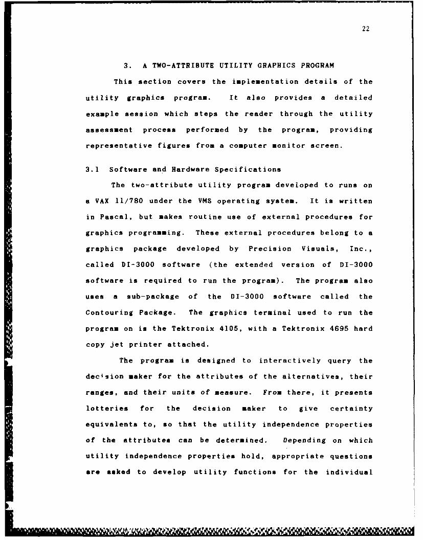
m oney (fig. 3.13). It is also a fairly realistic function

to apply except in cases where the decision maker's

certainty equivalents lie too close to the most and least

preferred consequence. If this is the case, the terative

optimization procedure for finding values for the b and c

variables does not converge to the specified maximum error

allowed by the program (.0001 units) within a reasonable

time (35 iterations), and the decision maker is informed

that his utility can not be assessed by the utility program

(fig. 3.14).

37

Figure 3.12 C.E. for Time Marginal Utility Curve Determination

Please enter your certainty equivalent for the "?": 30

Idt -.

I l-' I

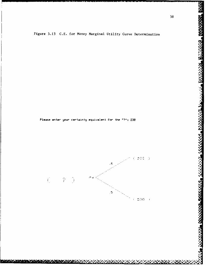
Figure 3.13 G.E. for Money Marginal Utility Curve Determination 3

U,

Jh

Please enter ylour certainty equivalent for the "2": 238 p'

'p

I'

op h

",'A

rv

S-

39

Figure 3.14 Program Inability to Assess Utility

The prespecifid curve used to approximate gour utilitycurve doesn't match gour values well enough to be used asan accurate representation. Urfortunateld, this programcan't be used to assess Uour utility. SORRY!

Hit a"~j ke followed b return to exit back to system level.

LowiQ&2r

40

If, on the other hand, the form can be used for each

attributes utility curve, it becomes necessary to determine

their scaling constants. One necessary condition is that

kv + kz + kyz = 1.

Here, kv is the scaling constant for the first attribute

(generically termed y) and kz is the scaling constant for

the second attribute (generically termed z). In the

additive independence case, kvz is 0 so that

ky + kz = 1.

We need to put kz in terms of ky or kv in terms of kz

to remove one unknown in the equation. This is done by

asking the decision maker to specify a preferred outcome,

either the (most preferred of attribute y, least preferred

of attribute z) or the (least preferred of attribute y, most

preferred of attribute z). Depending on the decision

maker's choice, if the first outcome is preferred, a value

for attribute y is sought to complete the indifference

relation. (fig. 3.15) (If the second outcome were

preferred, a -alue for attribute z would be sought, and if

the decision maker were indifferent between the two, the

utility values would already be available).

From this indifference value, it is possible to

establish the relationship between ky and kz (see Keeney

1976, pp. 278 - 281 for details), such as kz = .28kv or ky =

.36kz, etc. Finally, the last unknown must be solved for.

ell .A

41

Figure 3.15 Finding Scaling Relationship

In terms of the (HOURS , DOLLARS 3 outcome,Please enter sour preference.

166, 20) or ( 6, 300)

1) I prefer the outcome on the left.2) I prefer the outcome on the right.3) I am indifferent between outcomes.Choice: I

What amount of HOURS would make sou indifferent tothe outcomes below?

( ? , 200) , 300)amount of HOURS : 50

4

.... .

%t

42

This requires the decision maker to specify an outcome such

that it has a utility of 0.5.

The process of choosing this outcome is not handled

very elegantly in this program. Many possible combinations

of the two attributes exist which form a surface whose

utility value is 0.5. Ideally, a convergence technique to

help the decision maker focus on a particular outcome is

preferable. However, as it stands now, the decision maker

is faced with a direct assessment problem (fig. 3.16). This

results in a solution from the following equations (if, for

example, ky were .36kz):

ky = .36kz,

kvz = 1 - .36kz - kz, and

0.5 .36kz(Uy) + kz(Uz) + (I - .36kz - kz)(Uv)(Uz).

Since Uv and Uz are known because of their utility curves,

the only unknown is kz. Once kz is found, kv is found, and

then kvz. Keep in mind here that if additive independence

holds, kyz = 0.

Now the program fills an array with utility values for

possible outcomes of attribute y and z, and asks the

decision maker from which viewpoint he prefers to see the

utility graph (fig. 3.17 - 3.18). Then, depending on the

response, it draws one of eight graphs (here reflecting the

results of the example session answers for the mutual

utility independent case) (fig. 3.19 - 3.26). The other

possibilities for utility independence is utility

pq

43

Figure 3.16 Indiference Point Selection

In terms of the (HOURS , DOLLARS ) outcome,what values of HOURS (7) and DOLLARS (#)will make jou indifferent between the c.e. and the lottery?Value of HOURS : 38Value of DOLLARS 230

%.'.....

44

Figure 3.17 Representation of Viewpoints

This picture represents the viewpoints from which youcan look at your utility function.1)front 3)right 5 back 7) left2)front-riqht 4)back-right 6)back-left 8)front-leftHit the S Copyj key to 3et a hard copy of the picture.Hit any key followed by return to continue:

UTILITY

9' 5 4

-7 3

DOLLARS

* /i-- --- - ---

I

HOURSk --- - --- - - -

a45

Figure 3.18 Viewpoints Offered

V

Please indicate sour choice of viewpoint for the utilit graph.I)front 3)right 5)back 7)left2)front-right 4Jback-right 6)back-left S)front-left 9)quitchoice:

J '6

46

Figure 3.19 Viewpoint 1 (Example Session)

I

' 'IPOS

HOURS

47


48


. OWa

t 040

NDOLLARS

N * 911111 111) 11111 : 11

49


50


34. 00

11.

DOW

51

Figure ~ ~ ~ ~ ~ ~ 30 3.4VewonIO(xml Ssin

I

7.000


.il

FWWA

52


7. CO

S.000/

DL LAR S

53

Fiue3.26 Viewpoint 8 (Example Sessionl)

1

54

inc'ependence in one direction (either direction), or no

utility independence for the attributes.

3.2.2 Utility Independence in One Direction

If the responses for only one of the two attributes are

all equivalent (say for dollars) then the utility program

informs the decision maker (fig. 3.27) and obtains the

values necessary to develop the three marginal utility

curves (fig. 3.28 - 3.30). These curves are then combined

in the manner previously indicated (section 2.3.3) for

attributes utility independent in one direction. If none of

the previously mentioned properties exist, the fourth case,

of no utility independence between attributes, is chosen.

3.2.3 No Utility Independence

This case is indicated by non-equivalence of the

certainty equivalents obtained by asking the first ten

lotteries. Keeney (1976), however, has indicated it may be

possible to avoid taking a direct assessment approach

immediately by either transforming the problem attributes

into ones which do exhibit a form of utility independence,

or by decomposing the attribute ranges into subsets overI

which utility independence properties hold (fig. 3.31).

(Keeney 1976)1

If the decision maker chooses the first option, he is

expected to provide the transformed attributes and rerun the

%

55

Figure 3.27 Utility Independence One Way Indicated

Since your responses indicate that DOLLARS areutility independent of HOURSyour utility function can easily be assessed by developingthree marginal utility curves for the attributes. To do this,you will be shown additional lotteries for which ou mustenter your certainty equivalents.


56

Figure 3.28 C.E. for Money Marginal Utility Curve Determination

In terms of the (HOURS / DOLLARS ) outcome,please enter sour value for the "?": 230

3.--

Z 0 -- C.,

57

Figure 3.29 G.E. for Time Marginal Utility Curve Determination

(at Money min)

In terms of the (HOIJRS ,DOLLARS )outcome,please enter sjour value for the "':36

? 21:G1. 4..

Z ( t7.I. I

qkt

58

Figure 3.30 C.E. for Time Marginal Utility Curve Determination(at Moneymax )

In terms of the (HOURS / DOLLARS 3 outcome,please enter sour value for the "?": 70

-- 1 "

I , , I C

I-

V I,

Figure 3.31 No Utility Independence Indicated

Since your responses indicate that the attributes are not at allutility independent, there are three possible approaches toassessing utility values for the attributes. The first approachrequires you to rerun the utility program using transformedattributes which may exhibit utility independence. The secondapproach requires decomposing the attribute ranges andthen assessing the utilit function over these decomposedranges, which may be utility independent. Further guidance onthis option is provided when Vou choose it. Finally, thelast approach requires you to indicate your utilities directlyfor different combinations of attributes. Since this is themost difficult option to perform, it is recommended you tryone of the other two if possible.

Please indicate which option you want.1) Use transformed attributes.2) Decompose the attribute ranges.

3) Direct assessment.Choice: 2

--..- -.- rmww u

60

program (the program automatically restarts). If he chooses

to decompose the ranges, an explanatory paragraph gives an

example of how to do this (fig. 3.32) and he is offered a

chance to view his previous responses to the initial ten

lotteries (the answers are of the same form as those

presented during the consistency check). The utility

program is then restarted. Should the decision maker choose

the direct assessment option, he is warned about its

difficulty and told how to proceed (fig. 3.33). After that,

he is shown thirty six consequences over the attribute

ranges for which he must give his utility directly (fig.

3.34 - 3.39). In both the utility independent in one

direction and no utility independence cases, the same

viewpoints and graphs of the utility function are offered.

To show the applicability of even a simple two-

attribute utility program to a prototypical problem, we were

assisted by two Air Force officers from the 24th Air

Division, Griffiss AFB. They allowed us to assess their

utilities for tactical mission planning outcomes and the

sessions are recorded in the next section.

61

Figure 3.32 Decomposition of Ranges Chosen

Decomposing the attribute ranges should be done if thereis indication of utilitg independence over a subset of the range.This is indicated bg having a constant certaintg equivalent foran attribute even when the other attribute's value varies. Forexample, if your certainty equivalent for attribute one (rangingfrom, sag, 0 to 100) is always constant (sag, 60) over a subrange(sag, less than 350) of attribute two (ranging from, say, 200 to400), then a good place to subset the range would be from 200 to350 and 350 to 400. This wag, over the 200 to 350 range, someutilitV independence properties will hold.

Would you like to see your original answers again?1) yes2) noChoice: 2

Please indicate which operation you want to perform.1) Return to options menu.2) Perform the analysis over a subset of ranges.Choice: I

62

Figure 3.33 Direct Assessment Chosen

This procedure is difficult to perform because it is te-dious, and you must have a good feel for your preferences. Youwill be asked to assign a number from 0 to 1.0 to a variety ofoutcomes. Please think carefull about your choices.

Hit any key followed bj return to continue:

- .i

63

Figure 3.34 Direct Assessment Points 1-6

Based on the scale below, please enter the number tIou feelindicates the worth of the followtn5 Outcomes. The numberentered mat be real or integer between and including 0through I.e.

(TIME , MONEY

0, 28) s 8.82, 200) : 8.15

48, 20) 8 8.368, 20J : 8.480, 200) , 8.4510e, 201; 0.5

O.S I.0SI II IIHHII

64


(TIME MOHY

2, 22) a 0.340, 220) 0.456, 2-.0) s 6.45

60, 220) a0.5580, 22) 8 6.6ISO, 220) 6.65

I II II II I

65


(TIME ,MONlEY

0, 240) 0 .329, 240) 0 .4540, 240) 0 .660, 240) 0 .789, 248) 8 .75

160, 240) 8 .8

IN4I Iv I

al~inlr.N'

66


(TIME , MONEY8, 260) 0 .4

20, 260) 2 0.5540, 260) 0 0.7

60, 260) 8.8as, 260 : 8.85

18, 268) 0 0.9

0 1.0

67

Figrue 3.38 Direct Assessment Points 25-30

(TIME M FONEY8, 28) 0.45

29, 28) s 0.640, 2W6) 0 8.7566, 290) : 6.858o, 289) 0 6.91o, 280) 0 8.95

0 0.6 .I I II I I I I

I" I

68


(TIME ,MONlEY

6, 306) t 0.528, 360) t 6.65

40, 300) t 60.868, 306) 0 .9Be, 36) 6.95too, 306) a1.6

69

4. APPLICATION TO MISSION PLANNING

This section describes an attempt to determine the

utility graphs of two Air Force mission planners. The

process is described via figures of the computer screen

taken during the utility assessment session. A f ive step

approach is followed, in conjuction with running the

program, to perform the utility assessment.

4.1 Problem Discussion

The idea for applying the utility program to mission

planning arose from some research work being done for Rome

Air Development Center (RADC) at Griffiss AFB. There, in

the Decision Aids Section, a decision aid is being developed

to determine mission success based on a mission's

probability of arrival (Pa) to a target, and its probability

of destruction (Pd) of the target. The Pd for a mission is

readily available from the Joint Munitions Effectiveness

Manual, but the Pa is a fairly subjective assessment arrived

at from intelligence estimates of enemy threat. Since the

problem was characterized in this fashion, we decided it was

an ideal one for the utility program.

The two officers whose utilities were assessed were

Major Rand Case and Major Robert Stan. Both men had prior

experience in the mission planning area and are currently

assigned to the 24th Air Division, Live Exercise Division at

70

Griffiss AFB. To assess their utilities, the f ive step

process outlined by Keeney (Keeney 1976, p. 261) was used.

4.2 Five Step Assessment Procedure

This proceduro gives a systematic approach for assessing

utility, but there is no guarantee that following it results

in a correctly assessed utility function. the chances of

having a correctly assessed function increase if an

experienced analyst elicits the information from the

decision maker r the decision maker i s sufficiently

informed and comfortable with the ideas behind multi-

attribute utility theory. Since both officers were somewhat

familiar with the concept, and the computer program provided

the format to follow, the author hopes that my inexperience

as an analyst did not totally prejudice the process.

Following the five step process, we proceeded as follows.

4.2.1 Introduce Terminology and Ideas

Both officers were present at this part. We stressed

that it was not the kind of a problem where either of their

preferences were right or wrong, merely an indication of how

they felt about the problem at hand. We then asked if it

was reasonable to characterize tite problem of assigning

missions as being dependent on the two attributes Pa and Pd.

Both men felt it could be broken down into consequences of

this nature, but that while Pd was easily obtainable, Pa was

PS

V r r V wr r W

71

still a fairly ethereal concept. Bath agreed, however, that

if Pa could be determined, it would indicate, along with Pd,

the mission' s worth.

Since both men were familiar with the concept of

utility, we only had to familiarize them with the specific

terminology of the computer program as outlined in section

2.1. We also ran through an example session of the program

so they could see how it operated. We then asked Major Stan

to sit aside while we worked with Major Case.

4.2.2 Utility Assessment for Mission Planner I

To find the ranges of Pa and Pd over which to assess r6

his utility, we asked him if there were some value of Pa and

Pd below which he would never assign a mission. He said it

depended on the mission, and we asked him to think of a

specific type. He said fire suppression. His determination

was that no mission should be sent without at least a 45%

chance of arriving and a 25% chance of destroying the target

(fig 4.1). This meant the consequence -- in terms of (Pa,

Pd) -- for the least preferred was (45, 25) and most

preferred was (100, 100). The next step was performed byIthe utility program.Identify Relevant Independence Assumptions.

Major Case answered the initial ten lotteries (fig. 4.2

- 4.11). During this process, both he and Major Stan had

some problems. Initially, both officers wanted to enter the

72

Figure 4.1 Attribute Information

Please enter !our first attribute. If the attribute is over10 characters long, please abbreviate it to be 10 characters.

attribute name: PARRIVE

What units is this attribute measured in?: PA

Please enter the least and most preferred values this attributecan be -- (to the nearest whole number).

least preferred: 45most preferred: 108

Please enter sour second attribute. Again, please insure itdoes not exceed 18 characters in length.

attribute name: PDESTROY

What units is this attribute measured in?: PD

Please enter the least and most preferred values this attributecan have -- (to the nearest whole number).


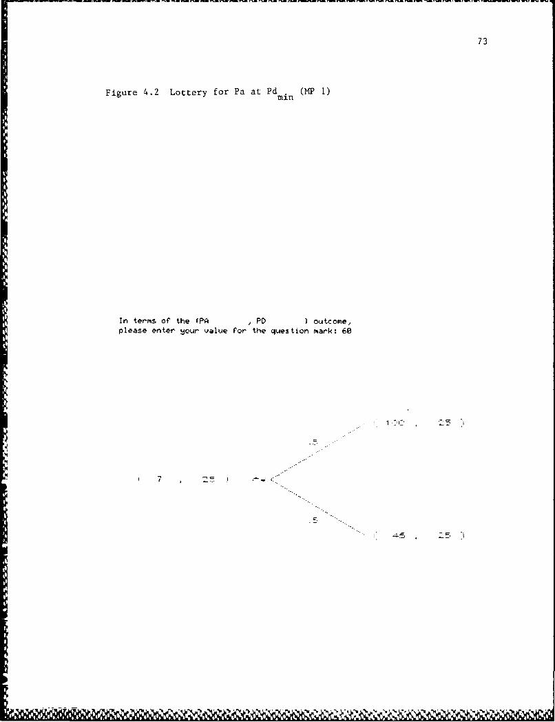
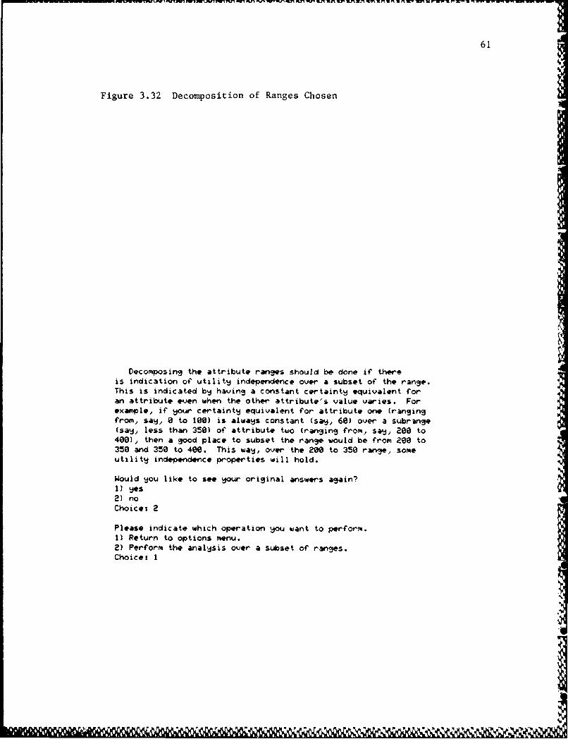
73

Figure 4.2 Lottery for Pa at Pdmin (MP 1)

In terms of the (PA / PD ) outcome,please enter your value for the question mark: 60

Z754=*1.

'4 7 ...

I--5..

74

Figure 4.3 Lottery for Pa at Pd (MP l)

In terms of the (PA , PD ) outcome,please enter !lour value for the question mark: 75

" 1, i fi1"

..-

... 5--'

75

Figure 4.4 Lottery for Pd at Pa mx(MP 1)

In terms of the (PA ,PD ) outcome,please enter !lour value for the question mark: 5S

17c

76

Figure 4.5 Lottery for Pa at Pd 2 5 (MP 1) I

In terms of the (PA , PD ) outcome,please enter sour value for the question mark: 55

. 1 ,-D 0 44

44 ) -

. 45 44 )

m

77

Figure 4.6 Lottery for Pd at Pa 5 0 (MP 1)

In terms of the (PA , PD ) outcome,please enter Wour value for the question mark: 50

I" 73 1 '0:

-7.3

(I 73 Z57

V 73, 25

Vt

78

Figure 4.7 Lottery for Pd at Pa (MP 1).25

In terms of the (PA , PD ) outcome,please enter !jour value for the question mark: 50

C C

I+ I

I

U.*~ p b.-YC S%. .- ,N

79

Figure 4.8 Lottery for Pa at Pd (MP 1)max

In terms of the (PA PD 3 outcome,please enter Vow value for the question mark: 69

C- 1

7 , 1i"Q ? ") -:: ..

"-,....

--,.

80

Figure 4.9 Lottery for Pd at Pa min (MP 1)

In terms of the (PA , PD 3 outcome,please enter sour value for the question mark: 50

45 1 C.

.,--

.5,

i" 45 25

81

Figure 4.10 Lottery for Pa at Pd 7 5 (MP 1)

In terms of the (PA , PD 3 outcome,please enter !jour value for the question mark: 79

,-5

.,--A

e -O V. 1

W "X...X

nwrw, mw Rn. w n iMm.l -Mn an.7lrp PM n w'w3.u N U w'u -W, M N r

82

Figure 4.11 Lottery for Pd at Pa (MP 1).75

V

In terms of the (PA , PD ) outcome,please enter gour value for the question mark: 50

o. C-"C.

.. S

°•S.

I .-C -I -

p

82

least preferred alternative as the certainty equivalent,

because they said they'd already indicated it was the

minimum acceptable amount. We had to reemphasize the nature

of the lottery being offered. We told them the worst they

could do was get the least preferred alternative, so how

much more would they have to get for certain before they

were willing to give up a 50% shot at the most preferred

alternative. Stated this way, they quickly realized the

intent of -he lottery. Major Case's data indicated that Pd

was utility independent of Pa (fig. 4.12).

Assess Conditional Utility Functions and Obtain Scaling

Constants.

Three points were elicited to develop the conditional

functions and scale the utility values (fig. 4.13 - 4.15).

After this, the eight different views of the utility graph

were plotted for him to see (fig. 4.16 - 4.23).'

Consistency Checking.

Major Case felt more comfortable being able to express

his preferences in words (as did Major Stan). He was

uncomfortable with some of his answers to the lotteries, but

was fairly confident the graphs showed his intentions to

give values for Pd without being influenced by Pa. Specific

comments on the technique by Major Case are included in

section 4.2.4.

-e .-e - .% .rt VrrF' *.- ***

83

Figure 4.12 Utility Independence One Way Indicated (MP 1)

Since Vour responses indicate that PD areutilitV independent of PAsour utilitV function can easilV be assessed bj developingthree targinal utilitq curves for the attributes. To do this,tou will be shown additional lotteries for which 5ou mustenter gour certainty equivalents.

Hit anj ke followed bj return to continue:

84

Figure 4.13 C.E. for Pd Marginal Utility Curve Determination (MP 1)

In terks of the (PA , PD ) outcome,please enter Vour value for the "7": 50

I' 4Z

* .-

O-iL97 276 DEVELOPMENT OF A GRAPHICS BASED TWO-ATTRIBUTE UTILITY 2/2ASSESSMENT PROGRAM W..(U) AIR FORCE INST OF TECHWRIGHT-PAITTERSON AFS OH E H MANNER DEC 96

UNCLASSIFIEDAFIT/CI/ NR-8-73? F/O 12/4 NL

mohEohhhEmoEEIEohhohhEEmhhEIEohmhmhhmhohEIsmmhhhohEEEmhsmmhmhohhhhEEmhhmhhhhhhhhmu

Wk.

0 I-k

w~~~ ,w .. 4 - w~

85

Figure 4.14 C.E. for Pa Marginal Utility Curve Determination (at Pd min )

(MP 1)

In terms of the (PA - PD ) outcopw,pleas enter sour value for the ?s: 75

5

86

Figure 4.15 C.E. for Pa Marginal Utility Curve Determination (at Pd max )(MPL )

In terms of the (PA , PD ) out:ome,please enter sour value for the s?": 50

? 1 , 1 c

' , 1-4'5 ,'1CC:

II _. -

- . ..

87

Figure 4.16 Viewpoinat 1 (MP 1)

88

Figure 4.17 Viewpoint 2 (MP 1)

10.

2.

7.

a

1.1

89


It.

.

a.

ta

P.

90


91


PD

92

Figure 4.21 Viewpoint 6 (B1

. 00

. W

93


MOOc

0.000

pe OCp

94


95

4.2.3 Utility Assessment for Mission Planner 2

Major Stan felt uncomfortable with the idea of setting

limits for Pa and Pd without knowing the specific mission,

as well. We asked him to think in terms of a specific

mission type as well, which made him feel better. His least

preferred consequences in terms of (Pa, Pd) was (60, 50) and

most preferred was (100, 100), (fig. 4.24).

Identify Relevant Independence Assumptions.

Major Stan's answers to the first ten lotteries (fig.

4.25 - 4.34) showed a possible inconsistency in his

certainty equivalents for Pd (fig. 4.35). When asked by the

program if this was intentional after being shown his

responses for the attribute certainty equivalents, he felt

it was; since at higher values of Pa his feelings about Pd

changed (fig. 4.16). This resulted in no utility

independence properties being present for the attributes

(fig 4.37). He chose to try to decompose the attributes,

and after viewing his original responses (fig. 4.38 - 4.40)

saw that Pa remained constant over all lower values of Pd

and only went down once the most preferred consequence of Pd

was reached. So, he indicated he'd like to perform the

analysis over a subset of the ranges (fig. 4.41).

This time, his consequence space for Pd changed. The

least preferred outcome remained constant, but he felt that

his preferences for Pa would only remain constant while Pd

was 90% or less. Therefore, his utility was assessed over

96

Figure 4.24 Attribute Information (1st try, MP 2)

Please enter !our first attribute. If the attribute is over

10 characters long, please abbreviate it to be 10 characters.

attribute name: PARRIUE

What units is this attribute measured in?: PA


least preferredt 60most preferred: 10e

Please enter Vour second attribute. Again, please insure itdoes not exceed 10 characters in length.



Plese enter the least and most preferred values this attributecan have -- (to the nearest whole number).


97

Figure 4.25 Lottery for Pa at Pd min (1st try, MP2)

In terms of the (PA , PD 3 outcome)please enter your value for the question mark: 80

,INN

"'.

I" 'I tI .I'

98

Figure 4.26 Lottery for Pa at Pd (1st try, MP 2).50

I n terms of the (PA ,PID )outcom,pleas" enter sjou value for the question mark: eO

* 75

99

Figure 4.27 Lottery for Pd at Pamax (1st try, MP 2)

In term of the (PA , PO 3 outcomep,please enter VoUr value for the question mark: 98

.. C " .DF....-

100

Figure 4.28 Lottery for Pa at Pd (Ist try, MP 2).25

In tors of the (PA , PD ) outcome,please enter our value for the question mark: 86

C...

Ik

101

Figure 4.29 Lottery for Pd at Pa (1st try, MP 2).50

1In temts of the (PA ,PD outcome,plea". enter Vour value for the question marks so

I C.C.

102

Figure 4.30 Lottery for Pd at Pa 2 (1st try, mP 2)

In terms of the (PA ,PO outcome,pleas* entr Vour value for the question marks 95

I 7iII-

7 1:1

103

Figure 4.31 Lottery for Pa at Pd mx(1st try, MP 2)

In terms of the (PA ,PD ) cutca"O,pleas. nter Vour value for the question marks 79

I D 1,1''0

gl5~

104

Figure 4.32 Lottery for Pd at Pami (Ist try, MP 2)ImiI

In terms of the (PA ,PD )outcome,please enter Vour value for the question marks 95

t:1 17

105

Figure 4.33 Lottery for Pa at Pd (1st try, MP 2).75

In terms of the (PA ,PO 3outcome,please enter gour value for the question marks 66

I 1~ ~ E-9

106

Figure 4.34 Lottery for Pd at Pa.75 (1st try, MP 2)

In terms of the (PA , PD 3 outcome,please enter Vow value for the question mark: 88

,._41J..

.5- "'" "" ".

7-

IN .'_

107

Figure 4.35 Possible Inconsistency Indicated (1st try, MP 2)

In terms of the (PA PD ) outcome, sinceVow responses for POESTROY all fall within 5 percent of the averaje,please carefull reconsider Uour previous answers. You willneed to determine if the attribute values should be changed to acomon value, and if so, which one. (NEXT SCREEN)

Hit " kevj followed bd return to continuea

108

Figure 4.36 Previous Responses for Pd C.E.'s (1st try, MP 2)

166, 88) ES.5( 166, 1I6) }0.5( 186, 50)]

80, 8) EO.5( 80, 106) 0.5( 80, 58)3

78, 95) E9C.5( 70, 186) e .5( 70, 50)]

60, 95) E8.5( 60, 1663 0.5( 60, 50)2

96, 8) E9.5( 96, 160) 0.5( 90, 56)3

Plea"e enter the, nuvm-e corresponding to gour choice.1) Change pe ious ansers to a comon one.2) Leav, answers as is.

Choices 2

~ %>

109

Figure 4.37 No Utility Independence Indicated (1st try, MP 2)

Since Vour responses indicate that the attributes are not at allutilitV independent, there e three possible approaches toassessing utilitV values for the attributes. The first approachrequires Vou to re-u the utilitq prog an using transformedattributes which ma exhibit utilit independence. The secondapproach requires decomposing the attribute ranges andthen assessing the utilitV function over these decomposedranges, which ma" be utilitV independent. Further guidance onthis option is provided Wh Wou choose it. FinallV, thelast approach requires Wou to indicate Vour utilities directljfor different combinations of attributes. Since this is themost difficult option to perform, it is recommended Vou trVone of the other two if possible.

Please indicate which option Wou want.1) Use transformed attributes.2) Dtcompose the attribute ranges.3) Direct assessment.Choice: 2

110

Figure 4.38 Decomposition of Ranges Chosen (1st try, MP 2)

Decomposing the attribute ranges should be done if thereis indication of utility independence over a subset of the range.This is indicated by having a constant certainty equivalent foran attribute even when the other attribute's value varies. Forexample, if your certainty equivalent for attribute one (rangingfrom, sa4, 0 to 100) is always constant (say, 60) over a subrange(sag, less than 30) of attribute two (ranging from, saj, 200 to400), then a good place to subset the range would be from 200 to350 and 350 to 400. This way, over the 200 to 350 range, someutility independence properties will hold.

Would you like to see your original answers again>1) yes2) noChoice: I

111

Figure 4.39 Previous Responses for Pa C.E.'s (Ist try, MP 2)

These are the choices made for PARRIUEb var-jing PDESTROY in terms of the

(PA , PD ) outcome:

30, SO) C0.5( le0. 50) 0 0.5( 60. 50)3

80, 75) C0.5( 100, 75) 0.5( 60, 75)]

80, 63) ~0.5( 100, 63) ; 0.5( 60, 63)]

70, 100) [0.5( 100, 100) 0 0.5( 60, 100))

C 80, 88) C0.5( 100, 88) ; 0.5( 60, 88)]

Hit anj keg followed by return to continue:

112

Figure 4.40 Previous Responses for Pd C.E.'s (ist try, MP 2)

These are the choices made for PDESTROYbj var-in3 PARRIVE in terms of the(PA , PD ) outcome:

80, 88) ~8.5( 88, 100) 0.5( 80, 58)]

70, 95) C~ .5( 78, 100) 0 0.5( 70, 50)]

60, 95) C0.5( 60, 100) 0 0.5( 60, 50)]

9, 88) C0.5( 90, 108) 0 0.5( 90, 50)]

Hit ang key followed bV return to continue:

113

Figure 4.41 Decomposition of Ranges Rechosen (1st try, MP 2)

Please indicate which operation jou want to perform.1) Return to options menu.2) Perform the anal,4sis over a subset of ranges.Choi0ce: 2

114

this lesser range (fig. 4.42). Now his responses to the ten

lotteries (fig. 4.43 - 4.52) indicated that Pa was utility

independent of Pd (fig. 4.53).

Assess Condi t ion al Utility Functions and Obtain Scaling

Constants.

After answering the questions used to build the

conditional utility curves (fig. 4.54 - 4.56), his graphs

were presented for him to see (fig. 4.57 - 4.64). He was

curious about how they could be used in an actual problem.

We explained how they could be compared between mission

planners and actual mission success to see which was the

best representation of utility, or how they could be

continually reassessed over time, depending on changing

conditions, and the progression of a decision maker's

preferences over time could be traced. Finally, the graph

represents information which will tell a decision maker

immediately if he prefers an outcome of (70, 80) or (75,

75).

Consistency Checking.

Major Stan felt good about the program's ability to

reflect his preferences. However, it was difficult to ask

specific questions about preferring particular outcomes

which were close together on the utility graph because of a

perspective distortion. This is a major critique item in

the next section.

115

Figure 4.42 Attribute Information (2nd try, MP 2)

Please enter Sour first attribute. If the attribute is over10 characters long, please abbreviate it to be 10 charcters.

attribute name: PARRIUE

What units is this attribute measured in' : PA



Please enter jour second attribute. Again, please insure itdoes not exceed 10 characters in length.



Please enter the least and most preferred values this attributecan have -- (to the nearest whole number).

least preferred: 50most preferred: 90Hit ang ke followed bq return to continue:

q

116

Figure 4.43 Lottery for Pa at Pdmin (2nd try, MP 2)

In terms of the (PA / PD ) outco",please enter Sour value for the question mark: 80

.......... . .. . .. . . . . . . . . . .

.7 !. - I ,- ' :"

....

.5 a,

117

Figure 4.44 Lottery for Pa at Pdmin (2nd try, MP 2)

In tr"s of the (PA PD ) outcoye,pleas enter sour value or the question ark: SO

-r 0

"-,S

1 18

Figure 4.45 Lottery for Pd at Pa mx(2nd try, MP 2)

I n torms of the (PA ,PO outcome,pleas. entr Vo..r value for the question~ tarks 78

I. 1 :IzI7

119

Figure 4.46 Lottery for Pa at Pd (2nd try, MP 2).25

1In trin of the (PA ,PD otoepleas. ente~r Ijow value for the question mark: 86

F-7 I

p. ~ pOf

120

Figure 4.47 Lottery for Pd at Pa 5 0 (2nd try, MP 2)

In term of the (PA P 3 outcome,pleas enter g value for the question mark: 78

V% .-"

121

Figure 4.48 Lottery for Pd at Pa.2 5 (2nd try, MP 2)

In terms of the (PA , PO outcome,please enter or value f#or the question parkg 88

7 T

.. I-

122

Figure 4.49 Lottery for Pa at Pd max (2nd try, MP 2) :

In term of the (PA ,PD u otc one,please enter' gour value for the question mark. 8@

, ~: i:4

123

Figure 4.50 Lottery f or Pd at Pa mn(2nd try, MP 2)

1In torsos of the (PA PD P outcome,pleas. enter gou value for the question mark 95

2 Q

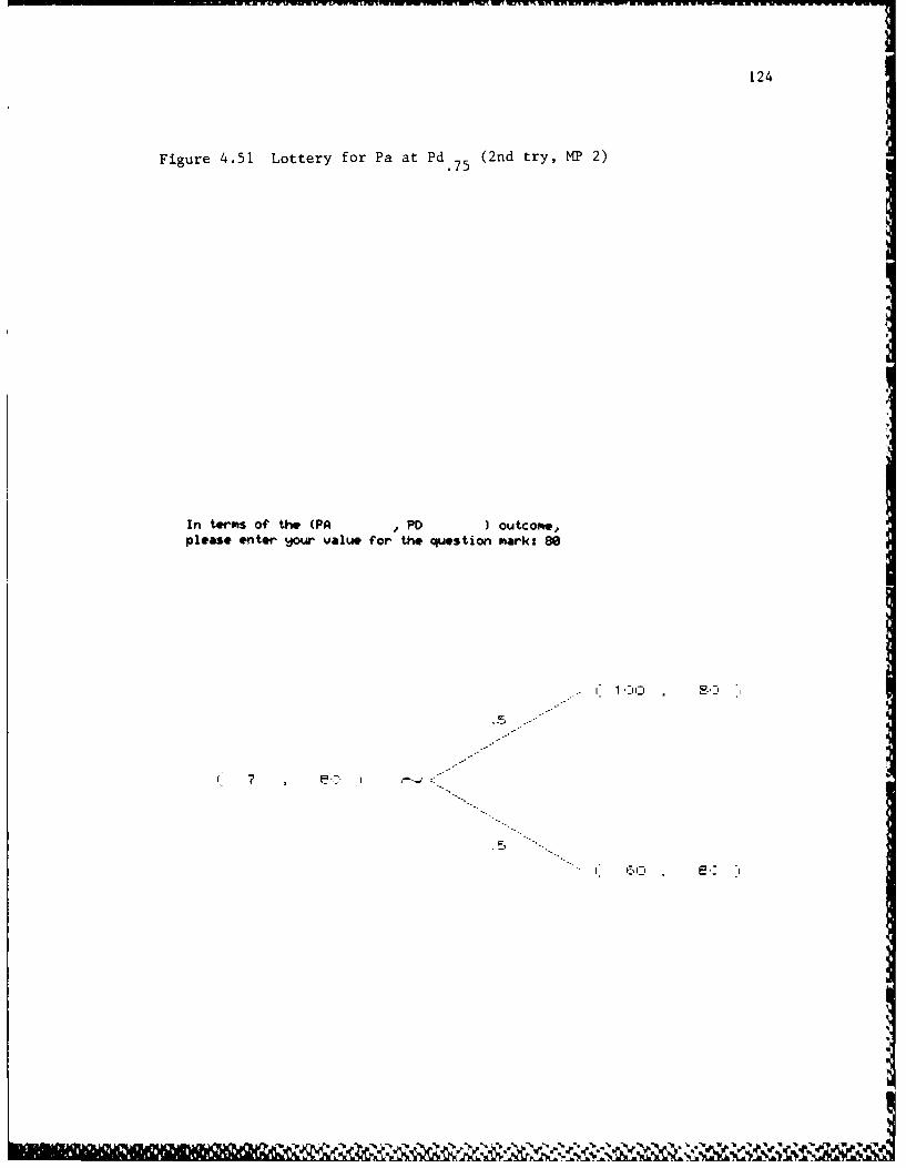
124

Figure 4.51 Lottery for Pa at Pd (2nd try, MP 2).75

In terms of the (PA , PD I outcome,please enter 9our value for the question mark: 8

. 1::. 2:

i. c-:"

7U

.. .. 5

6w-.

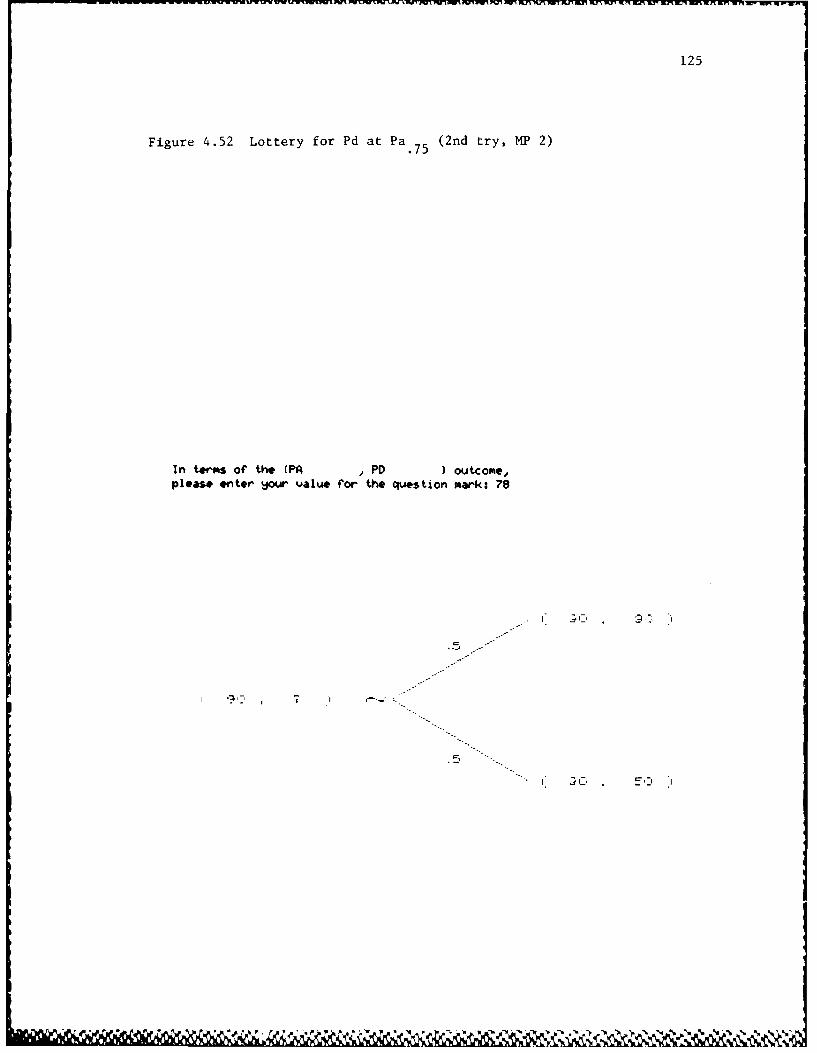
125

Figure 4.52 Lottery for Pd at Pa (2nd try, MP 2).75

In terms of the (PA , PD ) outcome,please enter jour value for the question mark: 78

I-"L

5,: I

126

Figure 4.53 Utility Independence One Way Indicated (2nd try, MP 2)

Since 4our responses indicate that PA areutilit4 independent of PD •Vour utilitt function can easild be assessed b developingthree marginal utilit4 curves for the attributes. To do this,4jou will be shown additional lotteries for which dou mustenter !Jor certaintV equivalents.

Hit anj ke followed b4 return to continue:

127

Figure 4.54 C.E. for Pd Marginal Utility Curve Determination (at Pamin)

(2nd try, MP 2)

In terms of the (PA , PD ) outcome,please enter !our value for the 8?":s0

I1 A o+- 5. I

(C V 0 ~ ~w . - go%--

-o.I

128

Figure 4.55 C.E. for Pa Marginal Utility Curve Determination (2nd try,MP 2)

In terms of the (PA , PO ) outcome,please enter sour value for the "?*: 80

.-" r ."L,_ D , =,- I j

"%",..° ..

15,

• , , . , . , . . . .. % € , % - , , , - " -?

129

Figure 4.56 G.E. for Pd Marginal Utility Curve Determination (at Pa ma)(2nd try, MP 2) a

In terms of the (PA ,PD) outcome,pleas. enter !jow~ value for the ~?z55

I ILI, ,

130

Figure 4.57 Viewpoint 1. (MP 2)

PA

11 5Si t11:111k a i

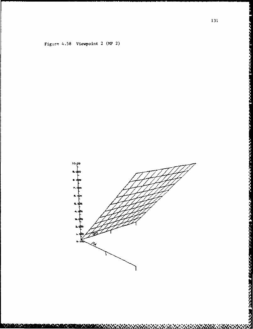
131


S.a

U.

7-

156

132

Figure 4.59 Viewpoint 3 (MP' 2)

I fk IRO

PA

133


AA

134


X 3..,

ro_ : "' .\- \" -am

7. 00C

AL 0-

IL

rk

,'%' ~ ~ ~ I PM4..' j ~

P% t%%%r

135


10. C*

a. od

7. coo

amo

%OGV

136


9. 001)

QCoo

&c.

.'F d

137


lei

f.A -P I$

138

4.2.4 Comments and Critiques

Both officers were impressed with the potential of

multi-attribute utility theory. Major Case, in particular,

had previously worked at trying to elicit preferences from

Tactical Air Force personnel, and was appreciative of the

structure the program lent to the process.

They both were concerned, however, over the

subjectiveness of the Pa attribute. An accurate model to

estimate Pa would have to be developed before reliance could

be placed on using it as an attribute.

Both officers commented on how they preferred a

technique which was representative of an individual's

preferences. It seems some expert systems are being

developed which are not powerful enough to assess situations

as well as humans, so nobody agrees with them. Multi-

attribute utility theory is flexible enough to be used in

these instances since rather than tell a decision maker what

to do, it merely maps his preferences for him.

The biggest problem, however, was one of information

portrayal. If, for example, the graphs had been presented

on a touch screen, it would have been possible to map pointsI

on the graph back to a specific utility. As it is now,

perspective effects make it difficult to find actual utility

value points.

% %Z% %

139

5. CONCLUSION

During the development of, and application of, the

utility assessment graphics program, a number of areas were

uncovered which need modification or expansion. Even so, we

feel the program has merit as a tool for practical problems

of choice involving only two attributes.

5.1 Extensions and Areas for Further Research

Based on our experience in developing and applying the

two-attribute utility program, the following areas are those

further work is needed.

The first extension is more of a modification. During

the course of the project, we grew increasingly frustrated

by the lack of flexibility of the DI-3000 graphics package

(in particular with the contouring package). Because the

specific application it was designed for was terrain

contouring, it was difficult to accomplish many things a

more generalized graphics package would provide. Also, as

mentioned earlier, hardware which allows user interaction

(suct as a touch screen, mouse, or joystick) for finding

utility values would prevent the perspective distortion

effects.

As for the program itself, its major areas of

additional work required are in the incorporation of more

pre-specified utility functions and consistency checking. A

consistency check for decision makers forced to use the

140

direct assessment option is desperately needed since the

process is so difficult to perform. A consistency checking

routine after the program is completed would be a nice

feature also. Since we mentioned the difficulty of direct

assessment, we shall reiterate the need for a procedure

which helps the decision maker focus in on the two-attribute

certainty equivalents that are required for scaling the

attributes.

There are also problems with the scale of the utility

axis on the utility graphs. They range from 0 to 10 instead

of from 0 to 1. This was due to the automatic labeling

function of the Contouring Package. Any future work should

insure the axis is labeled according to the 0 to 1 scale.

As a final extension, we would recommend the

incorporation of fuzzy attributes into the consequences.

Particularly in the case of mission planning, the use of a

fuzzy number for Pa is much more realistic. Good articles

on the topic of fuzzy decision analysis are (Litchfield

1976) and (Tong 1979).

5.2 Concluding Remarks

By now the benefits of multi-attribute utility theory,

even limited to the two-attribute case, are evident. The

ability to break a problem down into smaller ones has long

been advocated as a way of making it easier to solve (i.e.,

divide and conquer). In the same way, the use of this

141

methodology to develop a decision maker's utility is made

simpler by the exploitation of the four possible utility

independence properties. As is shown by the application of

even the simple program developed here to a real world

problem, multi-attribute utility theory forces a decision

maker to view a problem in the structured, consistent

fashion necessary to help him achieve a set of consequences

and their respective utilities. Once he has these

utilities, to make the best decision, he has only to

maximize expected utility to determine which alternatives to

choose.

In regard to what this project has meant to the author;

it has been a progression towards a fuller understanding of

the range and depth of utility theory This project has

deepened her perception of the field of decision analysis in

general, and has been a natural extension to her previous

work in the Decision Aids Section of RADC. As an Air Force

officer, being able to see the results of applying the

utility assessment graphics program to a real world problem

has been rewarding and the knowledge gained from this

experience can be used in future assignments. Finally, from

a computer systems standpoint, the ability to learn a new

editor and operating system (VAX 11/780), as well as using a

graphics package with which no previous experience was had,

has given the author an advantage in her next assignment

since their use will be required.

..* j -. ~,- ~ ~.f l

142

REFERENCES

Bolinger, J.J., Ghose, P., Sosinski, J.H., and Esser,W.F. 1978. Decision Analysis Utilizing MultiAttribute Utility Theory in Engineering Evaluations.IEEE Trans PAS. Vol 97 No 4:1245-1253.

Howard, R.A. 1968. The Foundations of Decision Analysis.IEEE Trans SSC. Vol 4 No 3:211-219.

Johnson, E.M. and Huber, G.P. 1977. The Technology ofUtility Assessment. IEEE Trans SMC. Vol 7 No 5:311-325.

Keeney, R.L. and Nair, K. 1975. Decision Analysis for theSiting of Nuclear Power Plants - The Relevance of MultiAttribute Utility Theory. Proc IEEE. Vol 63 No 3:494-501.

Keeney, R.L. and Raiffa H. 1976. Decisions with MultipleObjectives: Preferences and Value Tradeoffs. New York:John Wiley and Sons.

Litchfield, J.W., Hansen, J.V., and Beck, L.C. 1976. AResearch and Development Model Incorporating UtilityTheory and Measurement of Social Values. IEEE TransSMC. p. 400-410.

Sheridan, T.B. and Sicherman, A. 1977. IEEE Trans SMC. Vol 7No 5:392-394.

Spetzler, C.S. 1968. The Development of a Corporate RiskPolicy for Capital Investment Decisions. IEEE TransSSC. Vol 4 No 3:279-300.

Stimpson, W. 1981. MADAM: Multiple Attribute DecisionAnalysis Model, Vol I and II. Master's Thesis. AirForce Institute of Technology, WPAFB, OH. AD-AlIl 104and 105.

Tong, R.M. and Bonissone, P.P. 1979. Linguistic DecisionAnalysis Using Fuzzy Sets. Memorandum No UCB/ERLM79/72. Electronics Research Laboratory, College ofEngineering, University of California, Berkeley.

Worth, D.W. 1968. A Tutorial Introduction to DecisionTheory. IEEE Trans SSC. Vol 4 No 3:200-210.

143

APPENDIX

Program Listing

144

Programn draw(input, output);

label1restart;

canstattsize - 10;wrdsize - 40;stsize - 4;

tyjpeattribute - packed arrayll..attsize3 of char;wordstr -packed arra4Cl..wrdsiz@3 of char;parraj packed arrayCl:.itsize) of char;sarraqj varyjingCstsiz*J of char;range -integer;

lotrecord -record

attrib attributespas rangesans ranges

end;tarrai arrauj~l. . IO of lotrecordigtable =packed arrauil..11. 1.. 11J of real;worldarraj - packed arraujCl. . 3 of real;jstarray - arrauil. . 2 of integers

i :integer;attributel, attribute2 :attribute;minimumi. miniumum2, mauimumi. maximum2 :range;lottable :tarraizdellen. zratmin.ydellen. yratmin,udellen, sratmin. yb. zb. ujc, zc :real;widmin. wIdmax. eyje, at. zaxsbeg,zaxsend. sdoltik, idellab. idelbas.zdelpin, tskpval. yassbeg.yaxsend, ydoltik, yd*llab. ydelbas,ydolpln, Vskpval. xaxsbegoxaxsend, ideltik, idellab. xdelbas.xdelpin, zskpval worldarrajziabjst. ylabjst. alabjst :jstarrayiznminor, zlablfg, ynminor. ylablfg.xnminor. %lablfg integer;goon :boolean;rerun -option :integersattiscale. att2scalo attribute;

i These procedures are external to this program. They are written in 1,

< Fortran, and resident in the D13000 Software Graphics Package under 1,< VAX/VMS. )-

procedure JHSTRG(%stdoscr wstrg :wordstr); euterniprocedure JFONT~i :integer); extern;procedure JJVSTi j integer); *sternsprocedure JSIZE(x~y real); extern;procedure JOPEN) extern;procedure JROPEN(i :integer); @%terns

145

procedure JRCLOS(i : integer); extern;procedure JFRAME; ext ern;procedure JCOLOR(i integer); extern;procedure JLSTYL(i integer); extern;procedure JLWIDE(i integer); extern;procedure JCLOSE; externprocedure JBEQIN; extern;procedure JDINIT(i integpr); extern;procedure JDEVON(i integer); extern;procedure JVSPAC(w. i.y, z real); extern;procedure JVPORT(w,x.y,z real); extern;procedure JWINDO(w. x,y, z real); extern;procedure JMOVE(x,y : real); externiprocedure J3MOVE(x, y, z real); extern;procedure JPLANE(x.y,z real); extern;procedure JBASE(x,y, z real); extern;procedure JDRAW(x,y real); extern;

procedure JPAUSE(i integer); extern;procedure JSSINI; extern;procedure JSSPRO(m, n, e, a : worldarray); extern;procedure JSSAXS(m. n : worldarrag; z : real; a : integer; a worldarray;

y real; b integer; h : jstarray;p, q, r, s worldarray); extern;

procedure JSSMI(g gtable; 1, j, k : integer; m, n, o, p real;q integer; r : real); extern;

procedure JDEVOF(i integer); extern;procedure JDEND(L integer); externprocedure JEND; extern;

{ This is a macro to clear text from the dialog area )

procedure HOMEMN.CLEAR; extern;

(C INITGRAPHICS initializes the graphics devices used. a)

procedure INITGRAPHICS;begin

JBE I NjJDINIT(I )iJDEVO0N (1) ;

JVSPAC(-l.O. 1.0. -0.7, 0.7);JVPORT(-l.0. 1.0, -0. 7. 0. 7);JWINDO(O.O. 100.0, 0.0, 70.0);

end; (INITQRAPHICSI

-C **)W

(C ENDORAPHICS deactivates the graphics devices. 0.(C }

146

procedure ENDORAPHICS;beg in

JDEYOF(l)sJDEND (1);JEND;

end;

i* PUTVAL writes vall and va12 in the position determined by x and y. *)(* Values are surrounded by parentheses and separated by a comma. *)

{*************************-************************a**********************

procedure PUTVAL(x, y : real; vail, val2 parray);begin

,MOVE(X, ')i

JHSTRG(%stdescr '(');JMOVE(x + 1.0, y);HSTRG(%stdescr vall);

JMOVE(x + 11.0, y);JHSTRG(%stdescr ', ');JMOVE(x + 13.0. y);,JHSTRG(%stdescr val2);JMOVE(x + 23.0. y)iJHSTRG(%stdescr ")');

end; {PUTVAL)

(* PUTIVAL puts vall in place surrounded by parentheses, and val2 in a *)(* different place, also surrounded by parentheses. a)

procedure PUTlVAL(x, y : real; vall, val2 parray);begin

JMOVE(x, y);JHSTRG(%stdescr '(');JMOVE(x + 1.0. y);JHSTRG(.stdescr vall)iJMOVE(x + 11.0. y);JHSTRG(%stdescr ') ')JMOVE(0, y - 30.0)1JHSTRG(%stdescr '(')jJMOVE(x + 1.0. y - 30.0)1JHSTRO(%stdescr val2),JMOVE(x + 11.0, y - 30.0)1JHSTRG(%stdescr ')')i

end; (PUTIVAL)

(* CONVERT performs the conversion necessary to change an integer into a *)(9 string equivalent which can be printed by the JHSTRG procedure. *)(a .)

147

procedure CONVERT(intger integer; var turd parray);var

tamp *arrayi;begin

temp :~DEC(intger. stsize, 1); (DEC is a prodeclared pascal functijonj)turd :tamp;

end; (CONVERT)

(WRITEADOVAL prints the lottery values needed byj CHECKADDIND to deter- 5

(mine whether additive independence holds.

procedure WRITEADOVAI. maxl. min2, max2 integer; xpee. ypos real);var

smaxl, smax2,smini, smin2 :parray;

beginCONVERT(mazl, smaxi);CONVERT(mini, smint);CONVERT~max2, smax2);CONVERT(min2, smin2);PUTVAL(xpos, ypos, smaxi. smax2);PUTVALIxos ypos - 30.0. sminl. smin2);PUTVAL(xpos + 40.0. ypos. smaxl, smin2);PUTVAL(xpos + 40.0. ypos -30.0, sminl, smax2);

end; (WRITEADDVAL)

(a ETSTRING gets the particular values needed for lotteries in a varying a(aarray format. a

procedure GETSTRING(attl :attribute; minl, maxl. min2. max2 :range;var i :integer; var sl. s2, s3, s4, s5, s6 :sarreqst : tarray);

beginif tCI3. attrib - attl thenbeg in

ci : DEC(maxl, stsize, 1);s2 :DEC~t~i3.pos, stsite. 1);s3 :-DEC(minl, stsize. 1);%4- DEC(tCil.pos, stsire, 1);$5 :m ? 'is6 D EC(tCiJ. pos. stsize, I)

endelsebegin .

sl :DEC~tlI3. pos, stsize, 1);s2 :DEC~max2, stsie 1);13: DEC~tEi3.pos. stsize, 1)i14 :D EC(min2, stsize, 1);s5 :a DEC(t~fJ. pos. stsize, 1);

jjI

148

s6 : ? ? .,and;

end; {QETSTRING)

<. SETUP draws a lottery frame with .5's on it, but prints no values nor C)

(* reads the c.e.

procedure SETUP;var

strg : wordstribegin

JCOLOR(6);JSIZE(2.0, 2.0);4JUST(2, 2);JMOVE(65.0, 45. 0);JDRAW(40.0. 30.0);JDRAW(65.0. 15. 0);JJUST(1. 2);JMOVE(50.0. 40.0);JHSTRG(%stdescr ' 5');JJUST(1. 3);JMaVE(50.O, 20. 0);JHSTRQ(%stdescr '. 5');

JMaVE(35.0. 32.0);JSIZE(4.0, 4.0);JHSTRQ(%stdescr '1');

JSIZE(2.0, 2.0);end; (SETUP)

* DRAWLOT adds appropriate values to the lottery drawn by SETUP. The C)

(* c. e. 's are used to help determine independence properties. e)-C*

procedure DRAWiLOT(attl, att2 attribute; mini, mail, min2, max2 range;var index integer; tab : tarray);

varstrgl, strg2,strg3. strg4, strg5. strg : sarray;sl, s2 : parray;dummychar : char;x, y : real;

beginSETUP;GETSTRING(attl, mini, mail, min2, max2, index, strgl, strg2,

strg3. strg4, strgS, strg6, tab);JJUST(1, 2)jsI :- strg3;s2 :a strg4sPUTVAL(67.0, 15. 0, s1, s2);

sl .. strgS;s2 - strg6;

IU *q V 4.- "..

149

PUTVAL(5.0, 30. 0, sl, s2);

si strglis2 : strg2.PUTVAL(67.0. 45.0. %1, s2);

end; (DRAWLOT)

(* LOTTERIES has DRAWLOT present the lotteries, and it reads in the cer- *I

(* tainty equivalents For them into an arrayJ. .)

procedure LOTTERIES(attl, att2 attribute; minl, maxl, min2, max2-: range;var lottab tarray);

vara, i : integer;dummychar : char;

beginHOME_NCLEAR;for i :- 1 to 10 do

writeln;writeln(' You will now be shown a series of lotteries For which you');writeln('must enter your certainty equivalents: ');For i :- 1 to 5 do

writeln;write('Hit any keyj followed byj return to continue: ');

read ln(dummychar);HOMENCLEARINITGRAPHICS;a :- 0;for i 1 to 10 dobegin

a : a + 1;JOPEN;DRAWLOT(attl0 att2, minl, max1, min2, max2, a, lottab);JCLOSE;writeln('In terms of the (',attlscale.', ',att2scale, ') outcome,');write('please enter your value For the question mark: ');readln(lottablil. ans);JFRAAEiHOMEN_CLEAR;

end;

end; (LOTTERIES)

<* WELCOME is a short introductory paragraph to the program. *)

procedure WELCOME;

vari : integer;

dummychar : char;

4'%

150

beginHOME_N_CLEAR;for i :- I to 8 do

writeln;writeln(' This program is a generic multi-attribute utility theory');writeln('based methodology for assisting a decision maker. From inter-');writeln('acting with the decision maker, it will determine the decision');writeln('maker''s utility function over two user specified attributes. ');writeln( 'From there, it will present the utility function graphically, );writeln('at tte angle of rotation desired by the decision maker. ');for i :- I to 10 do

writeln;write('Please enter any character followed by a return to continue: ');read ln(dummjchar);HOMEN_CLEAR;

end; (WELCOME)

(* ATTRIBUTES asks the decision maker for his attributes and their *}{*ranges. *

procedure ATTRIBUTES(var attl,att2 : attribute; var minl, maxl, min2, max2range);

vari : integer;dummychar : char;

beginfor i :- I to 3 do

writelnwriteln(' Please enter your first attribute. If the attribute is over');writeln('lO characters long, please abbreviate it to be 10 characters. ');writelnwrite('attribute name: ');readln(attl);for i :- 1 to 2 do

writeln;write('What units is this attribute measured in?: ');readin~attlscale);for i :- 1 to 2 dowriteln;

writeln(' Please enter the least and most preferred values this attribute');writeln('can be -- (to the nearest whole number). ');writeln;write('least preferred: ')iread (mini);write('most preferred: ');readln(maxl)ifor i :- 1 to 2 do

writeln;writoln(' Please enter your second attribute. Again, please insure it');writeln('does not exceed 10 characters in length. ')swriteln;write('attribute name: ');readln(att2);for i :- I to 2 dowriteln;

151

writo('What units is this attribute measured in?: 1);readln(att2scale);fort i-I to 2 dowri taln;

writeln(' Please enter the- least and most preferred values this attribute');writeln('can have -- (to the nearest whole number). ');write in;write(least preferred-- ')iread (min2);write('most preferred:')read ln(inax2);writeC'IHit anyj keyj followed by~ return to continue: ');

read ln(dumamjchar);end; (ATTRIBUTES)

(a DEYTADLE builds a table of values for each attribute at (min. .25. .5. *3)(.75. and max) values.

procedure DEVTADLE~attI* att2 attribute; mini, maxl, min2. max2 :range;var table :tarraj);

beg intableCllattrib :- attl; (For example, tabletl2 will be used to add)tableC3. pos :- min2; (values to a lottery~ assessing the c. e. of)

(attribute 1 at attribute 2's minimum value)tablo[23.attrib :- atti;tabl*C23.pos :- ROUND((max2 - mmn2)/2 + min2);tableE33.attrib :- att2;tabieC33. pas :- mail;tabloE43.attrib :- attl;[email protected] :- ROUND((max2 - min2)/4 + min2);tabloECS.attrib :- att2jtableC53.pos :- ROUND((maxi - mini)/2 + mini);[email protected] :- att2;[email protected] :- ROUND(Cmaxl - minl)/4 + mini),tabl*C73.attrib :- atti;tableE73. pos :- max2;tabl*CS3. attrib :- att2.ltab l#CSJ.pos :- mini;tableC9.attrib :- atti;tablet9J.pos :- ROUND((Cmax2 -min2)/4) C3 + min2);tableCiO3.attrib :- att21tableEi03.pos :- ROUND((maxl -minl)/4) *3 + minli

end; (DEVTABLE],

(LOTFRAM1E is a generic procedure for drawing lottery angles. 0

procedure LOTFRAME(xcord. ycord, idlsp, ydisp :real);begin

JM'OVE(icord, ycord);JDRAW(xcord - xdisp. Ijcord - dlsp)iJDRAb(xcord, ycord - (ydisp a2))1

end; (LOTFRAMEI

152

* CHECKADDIND is used to present additional lotteries to determine if >

(* the additive independence property holds once mutual utility indepen- *>

{. dence has been determined. *)

C**C*************C***C**************************--***C******C*****

procedure CHECKADDIND(tab : tarray; ar addindep boolean);var

x, y : real;

choice : integer;aniwer, answer2 varying[33 of char;

beginJFRAME;HOMEN_CLEAR;JOPEN;JSIZE(2.0. 2.0);JCOLOR(6);LOTFRAME(20.0. 45.0, 15-0, 15.0);LOTFRAME(60.0, 45.0, 15:0, 15.0);JJUST(1, 1);x : 6.0;y : 37.0;

repeatrepeat

JMOVE(x, y);HSTRG(%stdescr '.5');

x :- x + 40.0;until x > 60.0;xU 6.0;y y - 14.0;JJUST(, 3);

until q < 23.0;x 21.0;y 45.0;

WRITEADDVAL(minimuml, maximum1, minimum2, maximum2, x, y);JCLOSE;writeln('With respect to the lotteries below, in terms of the');

writeln('(',attlscale, ', ',att2scale, ') outcome, please indicate '); h

writeln('which statement corresponds to your feelings about this lottery: ').

writeln('1) I am indifferent between the lotteries. ');

writeln('2) I prefer the lottery on the left. ');writeln('3) I prefer the lottery on the right. ');write('Choice: ');readln(choice)i

if choice - I thenaddindep : true

elseaddindep f false;

HOME_N_CLEARiJFRAME;

nd; CHECKADDIND)

153

I* UTIL finds the values of c and b which fit a utility function to the *>

0 decision maker's utility •>

procedure UTIL(maxt, cot real, var b, c real; sign integer);'aP

dumetchar char;

1, j, loop integerirmax, rimn,valnw real,continue booleane

oegin

c 0 5.S 0o;continue - true,reax . 1,rmin - O;while continue dobegin

valnw = 2 a (1.0 - EXP(sign a cmt * c)) - (1.0 - EXP(sign •maxt • c));if ABS(valnw) < 0.0001 then

begincontinue = false;b = I 0/(l 0 - EXP(sign a c * maxt));

endelse

begin

I i + 1);if i > 35 then pbegin

continue :- false;j - 1

end;if valnw > 0 then

rmal Celse

rein = C;c .- (rmax + rain)/2.0;

end;end;

C - c a sign;if j - I thenbegin

HOIE_N _CLEAR;for loop :- I to 5 do

writelnswriteln(' The prespecified curve used to approximate your utility');

writeln('curve doesn''t match your values well enough to be used as');

writeln('an accurate representation, Unfortunately, this program');writeln('can''t be used to assess your utility. SORRY!');

for loop :- 1 to 5 dowritelni

writeln('Hit any key followed by return to exit back to system level. ');readln(dummychar)iHALT;

end;end, (UTIL)

,--

154

(SCALE assesses the user's preferences between outcomes to determine a(the values for ky, kz, and kyz in the mnutuallyj independent and addi- a

(a* tive cases. In the additive case. kuji is automatically zero. a(a a

procedure SCALE(mode char; ymax, ijmin. zmax, zmin :integer; attl.&tt2 attribute;var kyj, kz, kyz: real; scaleyj, scalez, zb. yjb.zc, yc :real);

Vari, choice. yval,zval, yval2. zval2 :integer;symax, sijmin, szmax, szmin :parrayj;k, eql, eq2a, eq2b, eq3- eq4, tempk :real;

beginHOMIENCLEAR;for T :- 1 to 5 do

writein;writaln('In terms of the ('attiscale, '. ',att2scale.') outcome, ');writeln('Please enter yjour preference. ')jwrite in;writeln( ' ('. jmax. ', I, zmin, ') or C jymin. ', '. zmax. ') ;writein;writeln('1) I prefer the outcome on the left. ;writaln('2) I prefer the outcome on the right. ');writeln('3) I am indifferent between outcomes. ');writoC'Choice: )readln( choice);for £ :- I to 5 do

writein;if ((choice - 1) or (choice -3)) thenbegin J

writeln('What amount of '.attiscale. ' would make you indifferent to')writeln('the outcomes below?');wr i t en;writeln('( 7 ' zin. ') y'~min. ' .zmax '

write('amount of ',attiscale, ': ';-

adreadln(yjval);

alsobeg in

writeln('What amount of ',att2scale.' would make you indifferent to')writeln('the outcomes below?')iwrite in;writeln( 'C'. min. ', ? ) and C'. jmax *, '. zmin. ') ');write('amount of ',att2scale,': ')jread inCzval);

end;

HOME_ _C LEAR ILOTFRAME65.0, 45.0. 25.0. 15.0)iJJUST(1. 2);JMOVECS.O. 40.0);

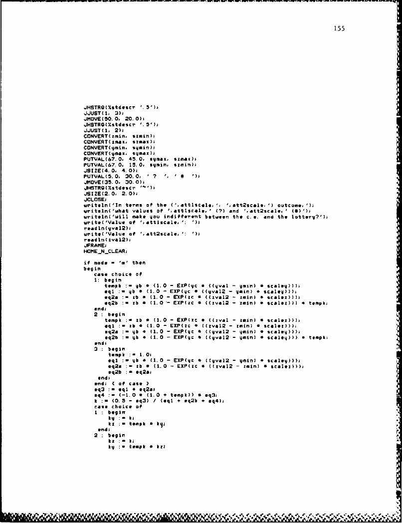
155

JHSTRG(%stdescr '. 5')1~JJUST(1. 3)jJMOVE(5O. 0. 20. 0)1JHSTRG(%stdescr '.5')1JJUST(I. 2)aCONVERT~zmin, szmin)iCONVERT(zmax, szmax);CONVERT(ymnn symin)iCONVERT(ymax, syJmax);PUTYAL(67.0. 45.0, sqjmax, szmax);PUTVAL(67.0. 15.0. sijmin, szim);JSIZE(4. 0. 4. 0);PUTVAL(5.0, 30.0, # ,' )

JA'IVE(35.0, 30.0);JISTR(%stdescr -')jJSIZE(2.0. 2.0);JCLOSE;writeln('Zn terms of the C',attlscale,', ',att2scale.') outcome,');writaln( 'what values of ',attlscal. ( ?) and ',att2scale.1 (*'wrjteln( 'will make yjou indifferent between the ce. and the lottery?');write('Value of ',attlscale ':')

read ln(ijval2);write('Value of '.att2scale, ':')read ln( zva 12);JFRAflE;140MEj4....LEAR;

if mode - 'in' thenbeg in

case choice of1: begin

tempk :- yb * (1.0 - EXP(ijc *((yyal - ymin) * scaleuj)));eqi : b *(1.0 - EXP(yc *((yval2 - min) s* aa))eq2a : b *(1.0 - EXP(zc *((zval2 - zmin) * scalez)));eq2b : b *(1.0- EXP(zc *((zval2 - zmin) * scalez))) *tempk;

end;2 :begin

tompk :- zb *(1.0 - EXP(zc *((zval - zmin) * scalez)));eqI z b C(1.0 - EXPOzC ((zval2 - mi) *scalem)));

eq2a : yb *(1.0 - EXP~yc *((yva12 - ymin) * scaleij)))eq2b : b a(1.0 - EXP(yc *((yval2 - ymin) * scaleyj))) *tempk;

and;3 :begin

tempk :- 1.0;eqi : yb *(1.0 - EXP(yc *((ijval2 - yjmin) * scaletj)));eq2a z b *(1.0 - EXP(zc *((zval2 - mi) *scalezm

eq2b : q2a;end;

end; (of case Ieq3 : qi * eq2a;eq4 :-(-1.0 * (1.0 + tempk)) *eq3;

k :- (0.5 - eq3) /(eqi + eq2b +~ eq4);case choice ofI :begin

km tempk k*end;

2 begin

ky tompk *kzI

156

end;3 : begin

k : k;kz : I, k.

end;end; -Cof case]-kqz : 1 .0- (kq + kz);

endelsebegin

eqI :- yb * (1.0 - EXP(qc * ((4val2 - min) e scale)));

eq2a : zb * (1.0 - EXP(zc * ((zval2 zmin) 4 scalez)));

if eqI - eq2a then

elseky 0.5

k: (0.5 - eq2a)/(eql - eq2a);

kz : 1.0 - ky;kqz : 0.0;

end;end; (SCALE)

(* UTILITY assumes a particular utility function, and determines the uti- )

- litiy of the input value-(of an attribute). C)

function UTILITY(val, b, c, scale : real; maximum, minimum integer):reol;

beginif val - 0 then

UTILITY :- 0else

if val - maximum thenUTILITY : 1.0

elseUTILITY : b * (1.0 - EXP(c C ((val - minimum) * scale)));

end; <UTILITY)

(* FILLARRAYS initializes the world coordinates' maximums and minimums. C)

(C It also locates the center of the mesh surface to be drawn (at array). >

procedure FILLARRAYS;var

I : integer;begin

for i :- I to 3 dobegin

~ '1 - r

157

wldminCi] : 0.0;wldmaxCi3 : 10.0;atci] "- 5.0;

end;end; {FILLARRAYS)

(* GETVIEW offers the user the choice of eight different viewpoints for C)

(* examining the mesh surface.

****CC**************C*********************C*****--**********

procedure GETVIEW(var choose : integer);begin

HOME N CLEAR;writeln('Please indicate your choice of viewpoint for the utility graph. ');writeln('l)front 3)right 5)back 7)left');

writeln('2)front-right 4)back-right 6)back-left 8)front-left 9)quit');write( 'choice: ');

readln(choose);end; (GETVIEW)

***e****--***************************.**********--************

(* ZAXSINIT initializes values needed to draw the z axis for the mesh *)

fC face. (for greater detail, see a DI-3000 Contouring User's Manual. ) *)

(C***C***C***********--**C********C**********C**************

procedure ZAXSINIT(var beg, endpt. tik : worldarray; var jst jstarray;var lab. skp : worldarray);

beginbegCl] : 0.0; (axis beginning)beg[2] : 0.0;begC3] : 0.0;endptCl3 :' 0.0; (axis ending)endptC2] : 0.0;endptC3] , 10.0;tik[1] :0 .5; (length and direction of tic marks)

tikC2] : 0.0;tikC3] : 0.01jst[1] : 3; (justification of tic marks and labels)

jst[2] :- 2;labEl3 : 0.71labC2] :- 0.0;

labC3] - 0.0;9kpCl] -20.0; (value to skip when adding tic marks - in)skpC2] * 20.0; (this case, none. }

skpC33 : 20.0;

end; (ZAXSINIT)

{* YAXSINIT performs the same function for the y axis as ZAXSINIT does C)

%N

158

< for the z axis. a)

procedure YAXSINIT(var beg, mndpt. tik : worldarray; vat jst jstarray;vat lab, bas, pln. skp worldarray; number integer);

begin

begCl] := 0.0;beg123 " 0.0;beg[33 : 0.0;endptC13 : 0.0;if number - 0 then

endptE23 : 10.0else

endpt121 : 5.0;endptC33 :- 0.0;

tikCl1 : 0.0;tikC23 : 0.0;tikC33 : -0.5;jstE13 : 2;jstC23 : 3;labC13 : 0.0;labC23 U 0.0;labC33 :- -0.7;basC13 : 1.0;bas[2] : 0.0;basC3] :- 0.0;plnCl3 : 0.0;pinC23 : 1 .0;plnC33 : 0.0;skpClJ : 0.0;skpC23 U 0.0;

skpC33 : 0.0;end; {YAXSINIT)

(a XAXSINIT performs the same Function For the x axis as ZAXSINIT does 4)

(* for the z axis. a)

procedure XAXSXNIT(var beg! endpt, tik : worldarray; vat jst jstarraq;var lab, bas. pin, skp warldarraj; number integer);

beginbegC13 : 0.0;

begC23 :, 0.0;begC3] : 0.0;if number - 0 then

endptC1] : 10.0else

endptC13 : 5.0;endptE23 : 0.0;endptC33 : 0.0;tikClJ :- 0.0;tik(23 : 0.0;tikC33 - -0. 5;jst[l3 : 2;jstC23 : 3j

labCl] : 0.01

159

labC2J : 0.0;labE33 -0.7;basEl3 :1.0;basE22 0.0;basE33 0.0;plnElJ 0.0;plnC23 1. 0;pln[3J : 0.0;skpEl3 0.0;skpC23 0.0;skpC:33 0.0;

end; -(XAXSINITI

(PLOTGRAPH draws the 3-D mash surface based on the user's choice of *-C* view. It also draws axe% for the mash surface. *Y

procedure PLOTGRAPH(choic-: integer; grid :gtab 1*; num: integer);var

i, j :integer;g :gtable;

beginfor i :- 1 to 11 do

for j :- 1 to 11 dog~i. j3 :- gridi, j3 * 10i (scales utility)-

(from I to 10)(for greater visibility]

(sets the viewpoint the user has specified>case choice of1 begin

@y&Cl3 U5.01

euieC23 -20.0;eqjeC33 U15.0;

zdelbasE13 tUzdalbasC2J : 0;zdelbasC33 Di0idelpln~l2 : 0zdwlplnE23 : 0zd~lplnC33 1;

end;2 begin

euje11i 30.0;euieC23 -20.0;

zdelbasC12 1;zdelbasC23 :1;zdalbasC33 : 0zdelplnCl3 :a 01idelplnC23 :- 01idolplnC33 i- I

end;5 begin

160

eyoeC13 5.0;e*eC23 30.0;eyeC33 15.0;zdelbasClJ :- -1;1zdelbasC23 0;zdelbasC33 0;zdelplnCl3 0;zdolplnC23 0;zdelplnC33 1;

end;8 begin

*qjeCl2 -20.0;oeje23 -20. 0;eijeC3 3 15.0;zdelbasClJ: 1zdalbasC23 1zdelbasC33 0;zdolplnE13 0;zdelplnC23 0;zdelplnC3] 1;

and;3 begin

eqeC13 30.0;eyjeC23 5.0;eyoeC33 15.0;zdolbasrl3 01zdelbasE23 : 1zdolbasE33 0;zdolplnC1I3 0;zdelplnC23 0;zdalplnC3J 1;

end;4 begin

ayE1e3 30.0;eyoeC23 30.0;weEC33 15.0;zdolbasE13 :- -1;E

zdalbasC33 U 0zdelplnCI3 0;zdelplnC23 0;zdalplnC33 ls1

end;7 begin

eyoC23 5.0;eqjeC33 15.0;

zdolbaC23 -1;zdelbasC33 : 0zdelplnElJ Os0zdelplnC2J : 0;zdoiplnC33 : 1

end;6 begin

eC13 -200;OeojeC23 30.OioejEC33 15.0;zdelbauCI] 1zdolbaeC23 1

161

zdelbasC33 :m 0zd*IpInEI3 0;zdelplnC2] 0; OzdolplnC33 1;.

end;end; (of case)ENDORAPHICS;if nun - 1 then

for0 -1 to 2 doeyje~i3 :- eyoli3/2;

JBEGIN;JDINIT( 1);JOE VON (1)5~JSS INI.JSSPRO(wlduin. widmat, eye., at);ZAXSINIT~zaxsbeg. zaxtend, ideltik, zlabjst. zdellab. zskpval);YAXSINIT(yassbeg, yaxsend. yd..ltik. ylabjst. ydollab, ydelbas, ydelpln,

yskpval. nun)iXAXSINIT(zaxsbeg, zaxsend, ideltik. slabjst. idellab. idelba, zdolpin.

xskpval, num);JOPENjJSSAXS(saxsbag. zaxsend. 1.0. 2. zdeltik. 0.5. 3. zlabjst,

zd*Llab, zdelbas, zdelpin, tskpval);JSSAXS(yaxsbeg, yaxsend. 5.0. 1. ydeltik, 0. 5. 0, ylab jst.

ydellab, ydelbas. ydelpln. yskpval);~JSSAXS(xazsbag, zaxsend. 5.0. 1. xdeltik. 0.5. 0. xiabjst.

xdollab. idelbas, xdelpin, iskpval);JCLOSE;

if nun - 0 then.JSSMI(g, 11, 11, It. 0. 0. 0. 0. 0. 0. 0.-0, -3. 1.0)

JSSMI(g. It, 6. 6. 0. 0. 0. 0. 0. 0. 0 0, -3. 1. 0);JOPEN;JSIZE(0.5, 0.5);if nun - 0 thencase choice of

1: beginJPLANE(0.0. 1.0. 0.5);J3MOVE(2.0, 0.0. 0.0);JHSTRQ(Xmtdescr attlscale);J3MOVE(-1.0. 9.0. 0.0)1JHSTRG(Xmtdoscr att2scale);and;

2: beginJPLANE(-1.0. 1.0. 0.5);J3MOVE(2.0. 0.0. 0.0);JHSTRO(Zstdoscr attlicale);JBASE(0.0. 1.0. 0.0);J3MOVE(0.0. 2.0. 0.0)1JHSTRG(%stdoscr &tt2scale);JBASE(1 0. 0.0. 0.0);and;

3. beginJPLANEC-1.0, 0.0, 0.5);JBASE(0- 0, 1. 0, 0.0O);J3MOVE(9.0. -1.0. 0.0);JHSTRG(%stdoscr mttlscalv),

162

J3MOVE(.0 0 2 0, 0.0);JHSTRQtstdttcr &tt2scale);JBASE(1.. 0. 0, 0. 0);end;

4: beginNJPLANE(-1.0. -1.0; 0.5)i

J3PIOVE(2.0. 0.0. 0.0);J.JUST(3, 1);,HSTRG(%hstdoscr attlscolo)iJJUSTC1, 1);JBASE(O. 0. 1. 0. 0. 0).J3lMaVE(0.0. 2.0. 0.0);,MSTRGCXstdescr att2scale);JDASE(1 0. 0.0. 0.0)1and;

5: beginJPLANE(0.0. -1.0. 0.5)jJ3tIOVE(2.0. 0.0. 0.0). e

JBASEC-1.0. 0.0. 0.0)1JJUST(3, 1);JHSTRG(%stdoscr attlscale)iJJUST(1. 1);J3MtVE(3. 0. 9 0. 0. 0);JHSTRQCVstdoscr att2scale);JBASE(1. 0. 0. 0, 0. 0);end;

6: beginJPLANE (1. 0. -1.0. 0. 5).jJASE(-1.0. 0.0. 0.0)1JJUST(3, 1);J3MOVE(2.0. 0.0. 0.0)1JHSTRG(%stdescr attlscale);JBASE-(0 0. -1.0. 0.0)1J3MOVE(0.0. 2.0. 0.0)1,.MSTRG(%stdoscr att2scale),JJUST(l. 1),JBASE(I.0. 0.0. 0.0O).end.

7: beginJPLANECI.0. 0.0. 0.5).JBASE(0.0. -1.0. 0.0),

J3r10VE(9.0. -3.0. 0.0).JHSTROC'Lstdoscr atti ecalo).J3MOVE(0 0. 2.0, 0.0).JH'STR(%stdeecr att2scale)iJJUST(1. 1).JBASE(1.0. 0 0. 0. 0). dend)

U: beginJPLAME(1.0. 1.0. 0.5)1J3MOVE(2.0, 0.0. 0.0),JHSTRG(Vstdoscr attlscale),

163

JBASE(0.0. -1.0. 0.0)jJJUST(3, 1)iJ3tIOVE(0.0, 2.0. 0.0).JHSTRG(%Stdescr att2scale);JJUST(1. 1);JBASE( 1.O. 0. 0, 0. 0);and;

end < castalsocase choice of

1: beginJPLANE (0.0, 1. 0, 0. 5);J3?OVE(1.0. 0.0. 0.0).JHSTRG(Xstdescr attiscale);J3MOVE(-0.5. 4.0, 0.0);JHSTRGCXstdoscr att2scale);end;

2: beginJPLANE(- 1. 0. 1. 0. 0. 5);J3MOVE(i.0. 0.0. 0.0);,MSTRG(VXstdoscr attiscale);JDASE (0. 0. 1. 0, 0. 0).j~J3M0VE(0.0. 1.0. 0.0);JHSTRGCstdescr a&tt2scale);JDASE(I. 0. 0. 0. 0. 01;and;

3: begin,PLANE(-1.0, 0.0. 0.5)1JDASE(0.0, 1.0. 0.0);J3MOVE(4.5. -0.5,. 0.0);JIISTrG(%stdoscr attlscale);J3MOVE(0.0. 1.0. 0.0)1JHSTRG(Ystdoscr att2scale);JBASE(1.0, 0.0, 0.0);endi

4: beginJPLANE(-1.0. -1.0. 0.5);JDASE(-1.0. 0.0. 0.0);J3MaVE(1.0. 0.0. 0.0)1JJUST(3, 1);J'STRQ(%Stdoscr attiscale);,JJUST(1. 1);JDASE(0.0. 1.0, 0.0);J3MOVE(0.0, 1.0. 0.0);J14STR(%stdescr att2scale);JOASE(1.0. 0.0. 0.0)1end;

5: beginJPLANE(0.0, -1.0. 0.5)jJ3P9OVE(1.0, 0.0. 0.0);t

JBASEC-1 .O 0.0. 0.0);JJUST(3. 1)iJHSTRGtStdoscr att iscale);JJUST(1, 1);

* 4N,%

-L'. CA 10W %.*V~.~ ~ .

164

J3MOVE(1.5. 4.5. 0.0);JHSTRGCstdoscr att2scale);~JBASE(1.0. 0.0. 0.0);end;

6 :*bginJPLANE(1.0 -1.0, 0.5);JDASE(-1.0. 0.0. 0.0);J.JUST(3, 1);J3MOYE(1.0, 0.0. 0.0).JHSTRGC%stdoscr attiscale);

J3tiOVEC0.0, 1.0. 0.0);JHSTRO(%stdoscr att2scale);JJUST(1. 1);JBASE( 1. 0. 0. 0. 0. 0);

nd;7: begin

JPLANE(1.0. 0.0. 0.5);JBASE(0.0. -1.0. 0.0);J.JUSTC3. 1);J3MOVE(4.5. -1.5, 0.0).JHSTRG(%stdoscr attiscale);J3MOVE(.0, 1.0. 0.0);JHSTRG(%stdoscr att2scale);JJUST(l. 1);

ow' JBASE(1.0. 0.0, 0.0);end;

% 8: begin% JPLANE(1.0 1.0. 0.5);

J3MOVECI.0 0.0. 0.0);JHSTRGCstdoscr attiscalt);JDASE(0.0, -1.0. 0.0);

* JJUST(3, 1);J3MOVE(.0, 1.0. 0.0);JHSTRG(%stdescr att2scale);J.JUST(1, 1);JBASE(I.0, 0.0. 0.0);and;

end; Ccase

,JCLOSE;end; (PLOTGRAPH>

(4 OXPIC is a representation of the different viewpoints from which the *)(*user can see his utility1 function. 4

procedure DOXPIC;var

dummychar : charibeg in

JOP EN a

----- ----- -~ --- ----- MUM -wW W W W W

165

JCOLOR ( I)JLWIDE(32767);JLSTYL (0);,JSIZE(2.0, 2.0)o~JMOVEC50.0. 56.0);JHSTRG(%stdoscr 'UTILITY');,JMaVE(53.0. 55.0)i,JDRAW(53. 0, 38. 0);JLSTYL (3);JORAW(53. , 18. 0);JDRAW(70.0, 18.0);JMOYE(53.0, 19.0);,JDRAW(58. 0, 26. 0);.JLSTYL (0).JPIOVE (70. 0, 19. 0);JDRAW(90. 0, 18. 0);JMOVE(82.0, 19.0);JHSTRGC%stds~r attlscale);JtIOVEC58.0. 26.0);JDRAWC64.0. 33.0);JPIOVE(66.0. 33.0);JHSTRG(%stdoscr att2scalt);JLWIDE( 16393);JCOLOR(6);JLSTYL (3);JtOVE(30.0. 10.0);JDRAW(30. 0. 30.0);JDRAW(45.0, 45. 0);

* JDRAW(75. 0. 45. 0);lsJDRAWC6O.0. 30. 0);1

JDRAkJ(60.0. 10. 0);JDRAW(75.0. 25.0)1JDRAW(45.0, 25.0);JDRAW(30. 0. 10. 0);JDRAW(60. 0. 10. 0);JPIOVE(75. 0. 25. 0);JDRAW(75.0, 45.0);JPIOVE(45.0, 45.0);JDRAW(45.0. 25.0);JMOVE(30.0. 30.0);JDRAW(60. 0. 30. 0);JLSTYL(0);JMOVE(45.0, 30.0);JSIZE(3.0. 3.0);JCOLOR(5);

9, JHSTRG(%stdoscr '1');JMOVE(60.0. 30.0);JHrSTRG(%stdoscr '2');JPIOVE(68.O. 38.0);JHSTRQ(%stdoscr '3');JPIOYE(75.0, 45.0)hJHSTRG(%stdoscr '4');JMOVE(60.0. 45.0);JISTRG(%stdoscr '5');JMOVE(45.0. 45.0);JISTRG(%stdoscr '6');JMOVE(38.0. 38.0)hJMSTRO(%stdoscr '7');JMOVE(30.0. 30.0);JMSTRQ(%stdoscr '8');

V

166

JCLOSE;writeln('This picture represents the viewpoints from which you');

writeln('can look at your utility function. ');writeln('l)#ront 3)right 5)back 7)left');writeln('2)front-right 4)back-right 6)back-left 8)front-left');writeln('Hit the S Copy key to get a hard copy of the picture. ');

write('Hit any key followed by return to continue: ');

readln(dummychar);nd; (BOXPIC)

(* FILLGRID fills an array with appropriate utility values based on the 4)

(4 given attribute values (y and z).

procedure FILLGRID(var grid : gtable; ky, kz, kyz, ycon, zcon, zb0 yb, zc,y€ : real);

vary, z, valy, valz : integer;

begin

for y :- 0 to 10 dofor z :- 0 to 10 dobegin

valy : ROUND((y/ycon) + minimuml);valz :- ROUND((z/zcon) + minimum2);grid[y + 1, z + 13 :- ky * UTILITY(val, yb, jc. ycon, maximum1,

minimuml)+ kz * UTILITY(valz, zb, zc, zcon, maaimum2,

minimum2)

+ kid * UTILITY(vaI, yb, yc, ycon, maximuml,

minimuml)

* UTILITY(valz, zb, ic, icon. maximum2, minimum2);

if gridCy + 1,z + 13 > 1.0 then (4 this check clips utility *)gridCy + 1,z + 1] :- 1.0 (4 values between 0 and *>

elseif grid[y + 1, z + 13 < 0.0 then

grid[l + 1,z + 13 :- 0.0;

end;end; (FILLORIDI

***********44*44*4444************4***********4**********4***4*****44*****

{* MUTORADD is used to gather additional data for developing the utility *)

(4 curve with UTIL once it's been determined that mutual utility indepen- 4)

(4 dence or additive independence holds. 4)

procedure MUTORADD(mode : char; tab tarray; var by, cy, cz, bz, cony ,

conz : real);var

continue . boolean,dummchar char;

r~n.~.'V'WVUlJ.. vw , U, ,1 n .f S 9 J fnnlnp,, Ita

167

ijaid. zm2d,ymaat, Zmaxt. cm.yt, cmzt :real;1, j, cm,. cmz, pick,yflag, zflag, ly. 1z, gnum integer;

smaz I ' mini. smin2, sma%2 parray;gridtabl * table;ki, k2, k3 .real;

beg inIfor i :- 1 to 15 do

iItel niwrxteln('Since your responses indicate that the');if mode - 'in' then

writaln('attributes are mutually utility independent,')else

writeln('attrjbutes are additive independent, ');

writoln('your utility function can easily be developed by assessing');writaln('the marginal utility curve for each attribute. To do this. ');writeln('you will be shown additional lotteries for which you must');aritoln('enter your certainty equivalents. ')i

for 1 :- I to 5 dowritel1 n.

write('Hit any key followed by return to continue:')read ln Cdummychar); ik

HOMENCLEAR;XJPEN;CONYERT~maximuml, smaxl);CONVERT(maximum2, smax2);CONYERT(ininimuml, sminl); W

CONVERT(minimun2, smin2);SETUP;IPUTIVAL(67.O. 45.0. smazi, sminl);JMOVE(5.0. 30.0);JSIZE(4.0, 4.0);JHSTRG(%stdescr 'C ? )')j.JSIZE(2. 0, 2. 0);JCLOSEi

write('Please enter your certainty equivalent for the '1?": ');

readinC cny );IJFRARE;SETUP;PUTIVAL(67.0, 45.0, smax2, smin2);JMOVE(5.0, 30.0);JSIZE(4.0, 4.0);

JHSTRG(%stdescr '( ? )')iI

write('Please enter your certainty equivalent for the "' )

read ln(cmz);JFRAME;cony :10. 0/(maximuil - minimuml)iconz 10. 0/(maxlimum2 - minimum2)i

:wax (maximumi - iinimuml) * cony;zmaxt : maximum2 - minimum2) * conz;cmyt :(cmy - minimuml-) *cony;cinit :(cmi - ininimuni2) acon:;ymid :(maximuml minimuml)/2;

I&~'J%.. -.. 7

168

zmid :- (magimum2 - minimum2)/2;yfiag :1;

if cmj < ymid thenjflag : -- 1;

if cmz < zinid thenzflag : -- 1;

if qflag > 0 thenUTIL(rjmaxt, cmijt, bq, cq, 1)

UTIL(ijmaxt, cmyt, byp cy, -1);if iflag > 0 then

UTIL~zmaxt. cmzt, bri cr. 1)

UTIL(zmaxt. cmzt, bz. cz, -1);SCALE(mode, maximumi. minimuml. maximum2, minimum2, attributel, attribute2,

hi. k2, k3, cony,. conz, bz, byj, zc, ijc)iFILLGRlD(gridtable, hi. k2, k3, cony,. conz, bz, by, zc. ijc);gnum :-0continue :- true,FILLARRAYS;HOMENCLEAR;%

HOME_N_ CLEAR;JFRAM'Eiwhile continue dobeg in

GETVIEW(pick);if pick <> 9 thenbegin

PLOTGRAPH(pick, gridtable, gnum);HOMEN_ CLEAR;

andelse

continue :- false;end;

*nd; <MUTORADDI

(ONEWAY fills the mesh surface arrayj grid in the case where the attri- *3.

btsatutilityj independent in one direction only. *

procedure ONEWAY~b _I. b 2. b_3, c 1. c 2. c 3. con_1. con 2 real;var grid g table; direction char);

vary, z: integer;valy, valz integer;

beg infor y :- 0 to 10 dobeg in

valy~ ROUND(C(j/con_2) + minimuml);for z :-0 to 10 dobeg in

valz :- ROUND((z/con_1) + minimum2)iif direction - 'z' th~en

gridEy + 1, z + 13: UTILITY(valyj. bR c_2. con_2, maximuml, z

4- W " r r J.dr."

169

minimum!) 4(I - UTILITY(valz. b 1I, c 1.conI. maximum2, minimum2)) + UTILITY(vahj.b 3, c_3. con_-2. maximuml, minimumi) *UTFILITY(valz, b_1. cil, con..1. maximum2,minimum2)

also

gridEj + 1, z + 13 UTILITY(valz, bi., ci. con 1. maximum2,minimum2) * (I - UTILITY~valy, b-2, c-2.con_2. maximumi. minimumi)) + UTILITY(valz,UTILlTY(valy, b_. c_2, con_.2, maximuml,minimum!);

end;end;

end; (ONEWAY)-

(~UTINDIWAY guides the pr ocess for drawing the mash surface when only *<* one of the attributes is utility independent of the other.

procedure UTINDIWAY(dir :char);var

continue :boolean;sinaxl smax2, smini, smin2 :parray;dummychar :char;ymid, zinid.bi. b2, b3, cl. c2, c3,conl, con2.cinit. cm2t, cm3t,maxit, max2t. max3t :real;pick,11. 12, 13.cml. cm2, c.3,flagi. flag2. flag3 :integer;gridtabl* gtable;dumscal*_A. duinscaleB :attribute;

beg inif dir - q' thenbegin

dumscale-A :attiscale;

edumscaleB :att2scale)

beginduinscaleA :att2scale;duiscaleI attiscale;

end;

HOME_NM_CLEAR;

for i :- 1 to 15 doIwritein('Since yjour responses indicate that ',duinscaleA.' are ')iwrlteln('utility independent of ',dumscale _B,'.');writoln('your utility function can easily be assessed by developing');writoin('three marginal utility curves for the attributes. To do this.,');

170

Writaln('Ijou will be shown additional lotteries for which yjou must');writoln('enter your certaintyj equivalents. ');

for i :- I to 5 dowr ite in;

write('Hjt anyj keyj followed byj return to continue: 1);read ln(dummychar);HOMEJJNCLEAR;JOPEN;CONVERT(maximuml, smazi);CONVERT~maximum2, smax2);CONVERT(minimumi. smini);CONVERT(minimum2, smin2);SETUP;PUTVAL(67.0. 45.0. smini, smax2);PUTVAL(5.0, 30.0, smini. ? ');PUTVAL(67.0. 15.0. sminl, smin2);JCLOSE;writeln('In terms of the ('.attIscale, '. ',att2scale. ') outcome.,,);write('please enter yjour value for the "?: )iif dir - 'z' then

readln(cml)else

read ln(cm2);HOME_N_CLEAR;JFRAME;

JOP EN;SETUPiPUTVAL(67.0, 45.0. smaxi, smin2);PUTVAL(5.0. 30.0, ? ', smin2);PUTVAL(67.0, 15.0, smini, smin2);JCLOSE;writeln('In terms of the C',attlscale. ', ',att2scale. ') outcome.,');write('please enter yJour' valu* for the ,?n: )

if dir -'z' thenree dinCc m2)

*ls*read ln(cml);

HOME_N_ CLEAR;JFRAMEi

JOPEN;SETUP;if dir - 'r' thenbeg in

PUTVAL(67.0. 45.0, smaxi, smax2);PUTVAL(5.0, 30.0, ? 7 , smax2);PUTVALC67.0. 15.0. sminl, smax2);

and*lSObeg in

PUTVAL(67.0. 45.0, emai, smai2);PUTVALCS.0, 30.0. smaxi. I ? ');PUTVAL(67.0. 15.0. smail. smin2);

end.~JCLOSEiwriteln('In terms of the ('attlocale. ', '.att2scale,') outcome,');write('please enter your value for the "7":')read in Ccm3);

1.71

HOME_N_CLEAR;JFRAME;

coni 10.0/(maximum2 - minimum2);con2 :10. 0/(maximuml - minimum!);

maxIt :(maximum2 - minimum2) * conl;max2t :(maximum! - minimum!) * con2;

if dir -'z' thenbegin

max3t U(maximum! - minimuml) * con2.cmlt U(cm! - mjnimum2) a cont;cm2t U(cm2 - minimum!) * con2;cm3t :(cm3 - minimum!) * con2;

andalsobegin

max3t U(maximum2 - minimum2) * con!;cmit :(cm! - miniwuml) * con2;cm2t :(cm2 - minimum2) a coni;cm3t :(cin3 - minjmum2) * con!.

end;

ijmid :(maximum! - minimumt)/2;zmid :(maximum2 - minimum2)/2;

flag! 1;flag2 : 1flag3 :1;

if cml < zmid thenflag! :- -1;

if cm2 < ymid thenflag2 :- -1;

if cm3 < ijmid thenflag3 :- -1i

if flag! > 0 thenUTIL(maxlt. cm~t, bi. cl, 1)

UTIL(maxlt, cm~t. bi. cl, -1);

if flag2 > 0 thenUTIL(max2t, cm2t, b2, c2, 1)

elseUTIL(max2t, cm2t, b2.# C2, '-1);

if flag3 > 0 thenUTIL(max3t. cm3t, b3; c3, 1)

elsoUTIL(max3t. cm3t, b3, C3, -1);

ONEWAY(bl. b2, b3. cl, c2, c3, con!, con2, gridtable, dir),FILLARRAYSHO)MENCL EAR;BOXPIC;H0MEN...LEARj

172

JFRAMEicortinue :- true;while continue dobegin

GETVIEW(pick);if pick <> 9 thenbegin

PLOTGRAPH(pick, gridtable. 0);HOME. _N_CLEARi

endelse

continue :- false;end;

end; CUTINDIWAYI

(* BOTHDEP guides the process for drawing the mesh surface when neither *)

C* attribute in utility independent of the other.

procedure BOTHDEP(var option : integer);var

i : integer;begin

HOME N CLEAR;for i :- I to 5 do

writeln;writeln('Since your responses indicate that the attributes are not at all');

writeln('utility independent, there are three possible approaches to ')i

writeln('assessing utility values for the attributes. The first approach');writeln('requires you to rerun the utility program using transformed');

writeln('attributes which may exhibit utility independence. The second');writeln('approach requires decomposing the attribute ranges and');

writeln('then assessing the utility function over these decomposed');writeln('ranges. which may be utility independent. Further guidance on');

writeln('this option is provided when you choose it. Finally, the ');writeln('last approach requires you to indicate your utilities directly ');

writeln('for different combinations of attributes. Since this is the '),

writeln('most difficult option to perform, it is recommended you try '),

writeln('one of the other two if possible. ');for I :- 1 to 5 do

writeln;writeln('Please indicate which option you want. ');

writeln('l) Use transformed attributes. ');writeln('2) Decompose the attribute ranges. ');writeln('3) Direct assessment. ');write('Choice: ');readln(option);HOME_N_CLEAR;

end; {BOTHDEP)

<* WRITEVALUES finds the correct values and prints them in the appropri- *)

(* ate position for the 5 lotteries shown to the decision maker in DRAW- *)

~ - ? e?. 01

173

(* CHECK.

procedure WRITEVALUES(C : chars x, q real; pos, ans, max, minparrayq);

varvell, vai2 : parraq;

beginif c - '' thenbegin

val : max;va2 : pos;

endelsebegin

vail : pos;vaiZ a max;

end;PUTVAL(x, y, vall, vai2);

if c s '' thenbegin

vail : ens;vai2 : pos;

endelsebegin

vail : pos;val2 : ans;

end;PUTVAL(x - 7.0 , - 10.0, vail, val2);

if c = 'y' thenbegin

vall :m in;val2 : pos;

endelsebegin

vail : po;val2 m sin;

end;PUTVAL(x, y - 20.0. vall, vae2);

vnd; (WRITEVALUES)

(4*4**44444*****444*44*4*444*4**** *4*4*}

(4 DRAWCHECK shows the decision maker his previous answers For c. e. 's to *)(4 help remedy possible inconsistencies.

(444444444****444444**444*44444**4*4*444*44**4*********4*)

procedur~e DRAWCHECK(ch :chars; table :terray);

1, vail, vai2, vei3, vai4,

vaiS, post. pos2, pas3, pos4,

I/1

174

po%5. ans, pot. max, min integer;X, y real;spas, sans. sinax smin :parray;

beg inif ch - ',j' thenbeg in

vail tabl*Cilans;posi tabieClJ.pos;val2 UtabloC23. antspas2 UtabloC23. pas;val3 :tabl@C43. ans;pos3 UtabloC43. possv&14 UtableC73.ans;

pos4 UtabloC73. passval5 tableC93.ans;pas5 tabl*EC9.pa,;max :tab loC33. pasimin: tableCS3. pass

write('(C'.vall:4. ', ',posi:4. ') CO.5 SC'max: 4, p a 'ps1: 4. '

writeln( '0.SC'. min: 4. ', '. posi: 4,writolnswrit@('(',val2:4, ', ',pos2:4,' 1 CO. S(',maz:4, '. '.pos2:4,. i

writeliwarit('(',val3:4. ', .,pos3.4.) ' * C. S('.max 4. '. '.pas3:4. ') ;wrsi tIn ( '. 5( '.min: 4,' .ps3: 4. ;writelnswrite('( ',val14:4. p aps4:4. r rc 5Cmax: 4, p pas4: 4, ;

wit. Inswrite('( , val5: 4, '. pos5: 4, CO. 5('.max:4, ''pos5: 4. 1;;

wri talniandelsebegin

vail tableC33. anespail UtabloC33. passvaI2 UtabloC53. ans;pas2 tabieCSJ. possval3 :-tabloC63.aonsspas3 :-tab leCd2. poe;val4 :-tabloCS3. ansppas4 -tab1839. passval5 table(103. ans;posS : tabl@ClOI. possmax :-tabloC73. passmin tablvCl). passwrite( (C', posl: 4. ', ', val1: 4.' CO. 5('ps. 4,' msa x: 4.')swriteln( 0.5SC ,posl:4 , ' ' ,min: 4. '

write in;writ@('('.pas2:4,. '.val2:4. ') - CO. SC'.pos2: 4.. ',max:4, 'writoln( 10. N ',pos2: 4,' 'min: 4'2)

write( '(C', pa,3: 4,. 'val3: 4, ) CO. SC'. pas3: 4. '.'max: 4.writeln('O.5('.pas3:4.', ',min:4, ')3')jwrite inswriteC 'C 'pos4:4. ', ',val4:4, ') ICO.5SC'.pos4:4., '.max:4. ') swriteln 'O. 5(', pas4 4. 1, ,min: 4. )3')1

175

wr ito In;s

write(lnC( .ps5: .pasS: 4 4' .sum: 4. '5 4, max 4,

wrijteins

end;

ends (DRAWCHECK>

(EXPLAIN explains how to decompose a user's ranges so the properties of *a)(4* utility independence mayj be used. It also offers the user a chance to *)(review his previous answers to lotteries, *)

procedure EXPLAIN(var continue boolean);var

i :integer;c: integer;dummejchar :char;

beg infor i :- 1 to 5 do

wr itel nwriteln(' Decomposing the attribute ranges should be done if there'),writeln('is indication of utilityj independence over a subset of the range. ');writoln('This is indicated byj having a constant certaintyj equivalent for ')swriteln('an attribute even when the other attribute''s value varies. For ');writeln('example, if your certainty equivalent far attribut* one (ranging');writeln('from, say, 0 to 100) is always constant (say, 60) over a subrange');writaln('Csay, less than 350) of attribute two (ranging from, say,. 200 to');writeln('400). then a good place to subset the range would be from 200 to');writoln('350 and 350 to 400. This way, over the 200 to 350 range, some');writaln('utilitj independence properties will hold. ');writeln;

writeln('Would yjou like to see your original answers again? 1);wrlteln( 11) yes');wrltaln('2) no');write('Choice; )read ln(c )sif c -1I thenbegin

HOME_N_ CLEAR;writeln('These are the choices made eor '.attributel);wrlteln('by varying ',attribute2, ' in terms of the');writeln('C'.attlscale,'. ',att2scale,') outcome: )wr itein;DRAWCHECK('y'. lottable)iWrite('Hit any keid followed bid return to continue: ')sreadln(dummychar )sHOME_N_CLEAR;wrltaln('Thest are the choices made $or ',attribut&2);wrlteln('by varying ',attrlbutel, ' in terms of the');writoln('(',attlscale,', '.att2scale,') outcome:')writelniDRAWCI4ECK('z', lottable)sWrlto('Hit any keyd followed bid return to continue: ')i

readln(dummdchar )s

176

HOMEJN_CLEARend;writeln;wr iteln;writeln('Please indicate which operation you want to perform. ');

writeln('l) Return to options menu. ');writeln('2) Perform the analusis over a subset of ranges. ');

write('Choice: );readln(i);if i - I then

continue : false

elsecontinue : true;

end; (EXPLAIN)

4 DRAWSCALE draws the scale for the user to look at while assigning uti- *}4 lity values to the outcomes.

***4***4***-*4********4**********4*******-****4***t********

procedure DRAWSCALE;var

i integer;a, x, y . real.c char;

beginJMOVE(10.0, 20.0);JDRAW(90.0, 20.0);JMOVE(IO.O, 25.0);

JHSTR(%stdescr '0');JMOVE(48. 0. 25. 0);

JHSTRG(%stdescr '0. 5'),JMOVE(85., 25.0);JHSTRG(%stdescr '1.0');

x : 10.0;y 23.0;repeat

JMOVE(x, q )JDRAW(x, y - 6.0);

x : x + 8.01until x - 98.0;

end; (DRAWSCALE)

***.44******44*******4***** ****4*444*****************4***4*44**

(- PRESENT presents a user with 36 different outcomes to assign utility 4)

(- values to.

4-44*f e**eee**4*e**e***t*****44e*********e****************4*4*t***

procedure PRESENTvar

gnum, pick,i, %, q. %step, jstep : integer;ivalues, yvalues : arrayjO..52 of integer;

0I

177

continue :boolean;

neginxstep :TRUNC((maximuml - minimuml)/5);ystep :TRUNC((maximum2 - minimum2)/5);zvalu@sl03 minimumiyvaluesC0J minimum2,-xvaluesClJ3 0;jvaluescl] 0;for i :- I to 5 dobegin

xvalues~i3 := valuesti - 1U + xstep;yvaluesCi3 y vdIuesCi - 12 + jstepi

end;INITGRAPHICS;JROPEN(1);~JCOLOR (4);~JFONT (3).,JSIZE(2.0. 2.0);JMOVE(50.0, 35.0);

4 DRAWSCALE;4 JRCLOS(1);

HOMENCLEAR;for i := I to 5 do

write in;wrjtaln('Based on the scale below, pleate enter the number .you feel');writeln('lndicates the worth of the following outcomes. The number ');

writeln('entered may bereal or integer between and including 0 ;writoln('through 1.0. ');for ± :- I to 3 do

writelifor y :- 0 to 5 dobeg in

writeln('(',attribute1,', ',attribute2, ')').for x :- 0 to 5 dobeg in

* write('(',xvalues~x3,', '.jvaluestjJ.')r *eadlIn~utilityx + 1, yj + 13); (save for mesh surface)

end;HOME N C LEAR;

end;ENDORAPHICS;gnu.. :- 1;continue : - true;for i :- I to 3 dobegin

wldmin ij 3 0. 0;wldmat~ij 5.0;atri3 :- 2.5;

* end;atC31 :- 5.0;wldmaxC33 :- 10,0;INITORAPHXCSiHOMENCLEAR.

HOMENCLEAR;

JFRAMIE;while continue dobeg in

-

a - s ~- . rW r IIF-7 J WUW WW W'AW'1WV 7 IIIY MM SrrrW . W ,- . .

178

QETVIEW(pick);if pick 40 9 thenbegin

PLOTQRAPH(pick, utility, gnum);HOME_NCLEAR;

endelse

continue :- falseiend;

end; {PRESENT)

{*-***********44.4****************************************************}

(* DIRECTASSESS introduces the direct assessment procedure.

* ***********************************************************************

procedure DIRECTASSESS;var

i : integer;dummychar : char;

begin

HOME_N_CLEAR;for i :- 1 to 5 do

writeln;

writeln(' This procedure is difficult to perform because it is te-');

writeln('dious, and you must have a good feel for your preferences. You');writeln('will be asked to assign a number from 0 to 1.0 to a variety of');writeln('outcomes. Please think carefullq about your choices. ');

for i :- I to 5 dowriteln;

write('Hit any key followed by return to continue: ');readn(dummychr);PRESENT;

end; (DIRECTASSESS}

<* TREND is used to uncover inconsistencies in a decision maker's re-

(* sponses. Possible inconsistencies are perceived to exist when all re-

{* sponses are close to, but not the same as, each other 5>

ftjction TREND(v, w, x, y, z : integer):boolean;

constpoint5 " 0.05;

vartotal, avg, fiveper : integer

beginTREND : true;total v + w + I + y + Z;avg :- ROUND(total/5)s

179 -

fiveper : ROUND((avg * pointS));if ((ABS(v - avg) < fiveper) and (ABS(w - avg) < fiveper) and

(ABS(z - avg) < fiveper) and (ABS(j - avg) < fiveper) and

(ABS(z - avg) < fiveper)) thenTREND :- false;

end; (TREND)

****411****4***********11***********14***********1414******1*********14-*1************41

(* CONSISCHECK reconfirms a decision maker's c. e. 's if inconsistencies *}

(4 are indicated. The decision maker may change the c.e. 's to a common *P<* value if desired, or, in the case of a trend, they may be left as is. *}

procedure CONSISCHECK(c : char;var choyse integer;var tab tarray);var

dummychar : char;val, i : integer;dumatt, dumscale : attribute;

beginif c - ' ' thenbegin

dumatt :- attributel;dumscale :- attlscale;

endelsebegin

dumatt :- attribute2;dumscale :- att2scal*;

end;HOMEN_CLEAR;for i :- 1 to 5 do

writeln;writeln(' In terms of the (',attlscale, ', ',att2scale, ') outcome, since ');write('Vour responses for ',dumatt, ' all fall within ');

writeln('5 percent of the average, ');

writeln('please carefully reconsider your previous answers. You will');writeln('need to determine if the attribute values should be changed to a')iwriteln('common value, and if so, which one. (NEXT SCREEN)');for i :- 1 to 10 do

writeln;write('Hit any key followed by return to continue: ');readln(dummychar);HOMEN_CLEAR;

DRAWCHECK(c, tab);writeln('Please enter the number corresponding to your choice. );

writeln(' 1) Change previous answers to a common one. ');writeln(' 2) Leave answers as is. ');write('Choice: '),

readln(chojse)i

if choyse - I thenbegin

write('What value would you like to change it to?: ');readln(val)Iif c - ,y, thenbegin

tabiti ans - val;tab[2].ans - val,tabC43 ans - vale

% % %-V

% %

N.~ ~ ~ ~ ~ ~ ~ ~ ~ ~ ~ ~~~~~~WW flW J J59U YXYM9.- M'.rMr, ' . ~P ~ ,.., ~ u, w% WrjW- WU WNT Nil Nil wWW wWu Nb W4Wv UNlR

1 80

tab[73. ans val;tab[93. ans vali

endelsebegin

tabE31. an. vafltabC53. an. val,tab[61. an. valDtabCS3. ans valitabClO). ans =val;

and;endi

and; CCONSISCHECK)

{ASSESSIND assesses which independence properties hold.

procedure ASSESSIND(var t :tarrarj);var

choice :integer;way : char;r~utindz., z _utind _r, addind, mutind boolean;scalerj. scalez :real;

beginr~utindj : false;xzutindr :-y false;mutind :false;

addind :false;if C(t~l3. an. - tE23.ans) and (tE43. an. - tC73. ins) and

(tC9].ans - t[13.ans) and (t[43.ans - ttlJ.ans)) thenVutind_z :- true;

if ((tC3]. ans -tE5J. ens) and (t[63. an. - tCS2. an.) and(t[lOJ. ans =tC33. an.) and (tC&J. an. tC33. ans) ) then

z _utindri :- true;

if not y utind z thenbeg in

if not TREND(ttl). ans. tE23. an.. t[43. ans tC71. an. tC93. an.)then

CONSISCHECK('rj'. choice, t);if choice - I then

rjutnd..z :- true;end;if not z _utind~y thenbegin

if not TREND(tC31.ans, tE53.ans, tE63.ans, tCB).ans, t[1O3 ans)then

CONSISCHECK('z', choice, t);if choice - I then

zutind.. :- truerend;if (rjutlnd _z and zutind~jj) thenbeg in

ASSESSMENT PROGRAM .. (U) AIR FORCE INST OF TECHRGHT-PATTERSO AFD OH E H WANNER DEC 86

UNCLASSIFIE AFTCI/NR-8-3 F/G 12/4 NLEu.

1.0 _ALA &L a32,-hA"&

~ mm..

181

mutind :- truesCI4ECKADDIND(t. addind)i

endsaif addind then

MUTORADD( 'a'. t, yb. ye. xc, zb, scaleys scalez)else

if mutind thenMUTORADD('m'. t. yb. yc. zc. ib, scaley. scale&)

elseif y~utindzt or zutindy thenbegin

If yutInd.. thenway : y'

alsoway :- 'i;

UTINDi WAY (way )iendelse

9OTHDEP (rerunoqption )sENDGRAP4ICSa

ends (ASSESSIND)

iMAIN PROGRAM)-

beginWELCOME;rerun..option :- 51 (rerun option of 5 means first time through),

restart: (label for place to return when restarting)if rerunoption - 2 then (it will if decomposition of ranges is needed),

EXPLAXN( go..on )if (gaoon) or (rerunoption - 1) or (rerunoption - 5) then

(either decomposition has been explained and the user wishes to continue(goon is true), or the user wants to use different attributes)(Crtrunoption is 1). or this is the first time through (rerun_.option)(c is 5).

beginATTRIDUTES(attributei. attribute2, minimumi. maximumi. minimum2. maximum2)aDEVTADLE(attributei. attribute2. minimumi, maximumi. minimum2, mauimum2,

lottable).LOTTERIES(attributels attribut*2, minimumi, maximuml, minimum2, maziaum2,

lottable);ASSESSIND( lottab Is),

(ASSESSIND will determine the independence properties. If none are I<present, the user will be asked if he wants to redo the program. If)<so, rerunopption will be either I or 2.

if (rerunoption a 1) or (rerunoption - 2) thengoto restarts

andelseif not go-on thenbegin

UOTHDEP(rerunoption)iif (rerunoption - 1) or (rerunoption - 2) then

goto restarts

182

andii# rerunapption -3 then

DIRECTASSESS;eind.

183

SDTTL HOMENCLEARESC - 27

HOME_.NCLR BYTE ESC.BYTE 37.BYTE 33.BYTE 49

.BYTE ESC

.ASCII 'Cli If'

.BYTE ESC

.ASCII 'roi'

.BYTE ESC

.BYTE 37

.BYTE 33

.BYTE 48

PSECT NONSHARED-DATA LONG, NOEXE, PICIOCHAN *LONG 0

TT *ASCID ITT'1083 BLKQ 1

PSECT CODE LONG, PICENTRY NOIIENMCLEAR.-M<1R2. R3.R4 R5. Rb R7. R. R9, RIO>

$ASSIGNS CHIAN - KOCHAN, DEVNAM - TT$QIOWS. CHAN - IOCHAN. -

FUNC - sloe lIRITEVULK. -

09 - I08.-PI - HM__L,P2 - *1. -P4 - #0

$DASSGN.S CHAN - IGOCHANRET*END

Mb

L-w-l.-M' . - -qw -,- .M -- A ew- - -w - -IF W qrJ4 vtV-

OF A GRAPHICS BASED TWO-ATTEIBUTE … 276 DEVELOPMENT OF A GRAPHICS BASED TWO-ATTEIBUTE UTILITY 1/3...

Documents

Transcript of OF A GRAPHICS BASED TWO-ATTEIBUTE … 276 DEVELOPMENT OF A GRAPHICS BASED TWO-ATTEIBUTE UTILITY 1/3...