Компьютерные,шахматы ... · Go AlphaZero AG0 3-day 31 – 19 AG0 3-day AlphaZero...

Компьютерные шахматы, компьютерное го и нейронные сети

А.С. Трушечкин

Конференция «Декабрьские чтения»

Новосибирск 22 декабря 2017 г.

•  Октябрь 2015: победа AlphaGo (Google DeepMind, Лондон) в матче против трёхкратного чемпиона Европы Фань Хуэя (5:0)

•  Март 2016: победа программы AlphaGo в матче по го против одного из сильнейших гоистов мира Ли Седоля (4:1)

•  Январь 2017: «таинственный игрок» Master на онлайн-‐площадках: 60 побед из 60 против сильнейших игроков мира

•  Май 2017: победа в матче против сильнейшего гоиста мира Кэ Цзе (3:0) и в партии против объединенной команды лучших китайских профессиональных игроков в го

•  Октябрь 2017: полностью самообучаемая программа AlphaGo Zero превзошла все предыдущие версии

•  1997: победа компьютера DeepBlue (IBM) в матче по шахматам против Гарри Каспарова (3,5:2,5)

•  Декабрь 2017: программа игры в шахматы AlphaZero поле 4 часа обучения победила одну из сильнейших программ Stockfish (64:36), которая, в свою очередь, превосходила сильнейших шахматистов-‐людей.

Game White Black Win Draw Loss

Chess AlphaZero Stockfish 25 25 0Stockfish AlphaZero 3 47 0

Shogi AlphaZero Elmo 43 2 5Elmo AlphaZero 47 0 3

Go AlphaZero AG0 3-day 31 – 19AG0 3-day AlphaZero 29 – 21

Table 1: Tournament evaluation of AlphaZero in chess, shogi, and Go, as games won, drawnor lost from AlphaZero’s perspective, in 100 game matches against Stockfish, Elmo, and thepreviously published AlphaGo Zero after 3 days of training. Each program was given 1 minuteof thinking time per move.

strongest skill level using 64 threads and a hash size of 1GB. AlphaZero convincingly defeatedall opponents, losing zero games to Stockfish and eight games to Elmo (see Supplementary Ma-terial for several example games), as well as defeating the previous version of AlphaGo Zero(see Table 1).

We also analysed the relative performance of AlphaZero’s MCTS search compared to thestate-of-the-art alpha-beta search engines used by Stockfish and Elmo. AlphaZero searches just80 thousand positions per second in chess and 40 thousand in shogi, compared to 70 millionfor Stockfish and 35 million for Elmo. AlphaZero compensates for the lower number of evalu-ations by using its deep neural network to focus much more selectively on the most promisingvariations – arguably a more “human-like” approach to search, as originally proposed by Shan-non (27). Figure 2 shows the scalability of each player with respect to thinking time, measuredon an Elo scale, relative to Stockfish or Elmo with 40ms thinking time. AlphaZero’s MCTSscaled more effectively with thinking time than either Stockfish or Elmo, calling into questionthe widely held belief (4, 11) that alpha-beta search is inherently superior in these domains.3

Finally, we analysed the chess knowledge discovered by AlphaZero. Table 2 analyses themost common human openings (those played more than 100,000 times in an online databaseof human chess games (1)). Each of these openings is independently discovered and playedfrequently by AlphaZero during self-play training. When starting from each human opening,AlphaZero convincingly defeated Stockfish, suggesting that it has indeed mastered a wide spec-trum of chess play.

The game of chess represented the pinnacle of AI research over several decades. State-of-the-art programs are based on powerful engines that search many millions of positions, leverag-ing handcrafted domain expertise and sophisticated domain adaptations. AlphaZero is a genericreinforcement learning algorithm – originally devised for the game of Go – that achieved su-perior results within a few hours, searching a thousand times fewer positions, given no domain

3The prevalence of draws in high-level chess tends to compress the Elo scale, compared to shogi or Go.

5

A10: English Opening D06: Queens Gambit8rmblkans7opopopop60Z0Z0Z0Z5Z0Z0Z0Z040ZPZ0Z0Z3Z0Z0Z0Z02PO0OPOPO1SNAQJBMR

a b c d e f g h

8rmblkans7opo0opop60Z0Z0Z0Z5Z0ZpZ0Z040ZPO0Z0Z3Z0Z0Z0Z02PO0ZPOPO1SNAQJBMR

a b c d e f g h

w 20/30/0, b 8/40/2 1...e5 g3 d5 cxd5 Nf6 Bg2 Nxd5 Nf3 w 16/34/0, b 1/47/2 2...c6 Nc3 Nf6 Nf3 a6 g3 c4 a4

A46: Queens Pawn Game E00: Queens Pawn Game8rmblka0s7opopopop60Z0Z0m0Z5Z0Z0Z0Z040Z0O0Z0Z3Z0Z0ZNZ02POPZPOPO1SNAQJBZR

a b c d e f g h

8rmblka0s7opopZpop60Z0Zpm0Z5Z0Z0Z0Z040ZPO0Z0Z3Z0Z0Z0Z02PO0ZPOPO1SNAQJBMR

a b c d e f g h

w 24/26/0, b 3/47/0 2...d5 c4 e6 Nc3 Be7 Bf4 O-O e3 w 17/33/0, b 5/44/1 3.Nf3 d5 Nc3 Bb4 Bg5 h6 Qa4 Nc6

E61: Kings Indian Defence C00: French Defence8rmblka0s7opopopZp60Z0Z0mpZ5Z0Z0Z0Z040ZPO0Z0Z3Z0M0Z0Z02PO0ZPOPO1S0AQJBMR

a b c d e f g h

8rmblkans7opo0Zpop60Z0ZpZ0Z5Z0ZpZ0Z040Z0OPZ0Z3Z0Z0Z0Z02POPZ0OPO1SNAQJBMR

a b c d e f g h

w 16/34/0, b 0/48/2 3...d5 cxd5 Nxd5 e4 Nxc3 bxc3 Bg7 Be3 w 39/11/0, b 4/46/0 3.Nc3 Nf6 e5 Nd7 f4 c5 Nf3 Be7

B50: Sicilian Defence B30: Sicilian Defence8rmblkans7opZ0opop60Z0o0Z0Z5Z0o0Z0Z040Z0ZPZ0Z3Z0Z0ZNZ02POPO0OPO1SNAQJBZR

a b c d e f g h

8rZblkans7opZpopop60ZnZ0Z0Z5Z0o0Z0Z040Z0ZPZ0Z3Z0Z0ZNZ02POPO0OPO1SNAQJBZR

a b c d e f g h

w 17/32/1, b 4/43/3 3.d4 cxd4 Nxd4 Nf6 Nc3 a6 f3 e5 w 11/39/0, b 3/46/1 3.Bb5 e6 O-O Ne7 Re1 a6 Bf1 d5

B40: Sicilian Defence C60: Ruy Lopez (Spanish Opening)8rmblkans7opZpZpop60Z0ZpZ0Z5Z0o0Z0Z040Z0ZPZ0Z3Z0Z0ZNZ02POPO0OPO1SNAQJBZR

a b c d e f g h

8rZblkans7ZpopZpop6pZnZ0Z0Z5ZBZ0o0Z040Z0ZPZ0Z3Z0Z0ZNZ02POPO0OPO1SNAQJ0ZR

a b c d e f g h

w 17/31/2, b 3/40/7 3.d4 cxd4 Nxd4 Nc6 Nc3 Qc7 Be3 a6 w 27/22/1, b 6/44/0 4.Ba4 Be7 O-O Nf6 Re1 b5 Bb3 O-O

B10: Caro-Kann Defence A05: Reti Opening8rmblkans7opZpopop60ZpZ0Z0Z5Z0Z0Z0Z040Z0ZPZ0Z3Z0Z0Z0Z02POPO0OPO1SNAQJBMR

a b c d e f g h

8rmblka0s7opopopop60Z0Z0m0Z5Z0Z0Z0Z040Z0Z0Z0Z3Z0Z0ZNZ02POPOPOPO1SNAQJBZR

a b c d e f g h

w 25/25/0, b 4/45/1 2.d4 d5 e5 Bf5 Nf3 e6 Be2 a6 w 13/36/1, b 7/43/0 2.c4 e6 d4 d5 Nc3 Be7 Bf4 O-O

Total games: w 242/353/5, b 48/533/19 Overall percentage: w 40.3/58.8/0.8, b 8.0/88.8/3.2

Table 2: Analysis of the 12 most popular human openings (played more than 100,000 timesin an online database (1)). Each opening is labelled by its ECO code and common name. Theplot shows the proportion of self-play training games in which AlphaZero played each opening,against training time. We also report the win/draw/loss results of 100 game AlphaZero vs.Stockfish matches starting from each opening, as either white (w) or black (b), from AlphaZero’sperspective. Finally, the principal variation (PV) of AlphaZero is provided from each opening.

6

Расчёт vs Интуиция

Александр Динерштейн, 7-‐кратный чемпион Европы по го: «Для меня это остаётся большим вопросом – как будет действовать программа, если с первых же ходов свернуть с дебютных справочников. На пустой доске вариантов столько, что никаким методом Монте-‐Карло их не просчитать. В этом го выгодно отличается от шахмат. В шахматах всё давно изучено на глубину 20-‐30 ходов, а в го, при желании, уже первым ходом можно создать позицию, которая не встречалась в истории профессионального го. Программе придётся играть самостоятельно, а не вытаскивать варианты из базы знаний. Посмотрим, сможет ли она это сделать. Я в этом сильно сомневаюсь и ставлю на Ли Седоля».

Стоя на плечах гигантов… •  Первая программа игры в го – 1960

•  Непосредственно перед AlphaGo: программы на уровне мастеров-‐любителей

•  Но был большой разрыв в силе игры с профессионалами

•  А. Динерштейн: «Я был уверен, что у нас есть хотя бы 10 лет в запасе. Ещё пару месяцев назад мы играли с программами на форе в четыре камня – это примерно как фора в ладью в шахматах. И тут – бац! – и сразу Ли Седоль повержен».

Шашки, шахматы, го – это игры со следующими свойствами:

•  С полной информацией •  Антагонистические (с нулевой суммой) •  Конечные

Дерево игры 4

2 -‐3 4

2 5 -‐2 -‐3 5 4

0 2 3 5 -‐4 -‐2 -‐5 -‐3 -‐1 4 5 1

MAX

MAX

MIN

•  Число всевозможных партий ≈ bd o b – средний коэффициент ветвления (число возможных ходов в фиксированной позиции)

o d – средняя глубина дерева (длина игры) •  Шахматы: b≈35, d≈80, bd ≈ 10124

•  Го: b≈250, d≈150, bd ≈ 10544 •  Число атомов во Вселенной: 1080

Вариативность шахмат и го

Альфа-‐бета-‐отсечение 4

2 ≤-‐2 4

2 ≥3 -‐2 ≥5 4

0 2 3 -‐4 -‐2 -‐1 4 5

MAX

MAX

MIN

Применение альфа-‐бета-‐отсечения •  Итак, каждая вершина (состояние игры) s имеет свою ценность v*(s) – выигрыш одного из игроков при оптимальной игре обоих

•  Рассчитать на несколько ходов и вычислить оценку v (s) ценности терминальных позиций – Пример в шахматах: оценка материала (пешка – 1 очко, конь и слон – по 3 очка и т.д.)

–  В DeepBlue – сложная экспертная формула оценки позиции (8000 параметров)

•  Итеративное углубление –  В DeepBlue: углубление на от 6 до 16, в отдельных случаях – до 40 уровней

•  Проблема: в го, помимо большего объёма перебора, сложно формализовать качество позиции

Машинное обучение

«Область исследований, изучающая возможность компьютеров обучаться без непосредственного программирования» (Артур Сэмюэль)

В.Н. Вапник, А.Я. Червоненкис, Ю.И. Журавлёв

Нейронные сети

При большом количестве слоёв – «проклятие размерности»

Нейронные сети глубокого обучения (deep learning), с середины 2000-‐х

Устройство AlphaGo Zero •  Анализ дерева методом Монте-‐Карло: рассматривать не всё дерево, а только перспективные ходы.

•  Перспективные с точки зрения нейронной сети

•  Оценка позиции также дается нейронной сетью

•  Более глубокое рассмотрение перспективных вариантов

Метод Монте-‐Карло для поиска в дереве

•  Дерево формируется итеративно •  Начальное дерево – текущая позиция •  На каждой i-‐й итерации дерево проходится от корня до некоторого листа, который затем разветвляется.

•  Нейронная сеть выполняет оценки априорного качества каждого нового хода 0≤P≤1 и оценку ценности –1≤V≤1 каждого нового листа

(V = 1 – 100% выигрыш, V = –1 – 100% проигрыш).

ARTICLE RESEARCH

1 9 O C T O B E R 2 0 1 7 | V O L 5 5 0 | N A T U R E | 3 5 5

repeatedly in a policy iteration procedure22,23: the neural network’s parameters are updated to make the move probabilities and value (p, v) = fθ(s) more closely match the improved search probabilities and self-play winner (π, z); these new parameters are used in the next iteration of self-play to make the search even stronger. Figure 1 illustrates the self-play training pipeline.

The MCTS uses the neural network fθ to guide its simulations (see Fig. 2). Each edge (s, a) in the search tree stores a prior probability P(s, a), a visit count N(s, a), and an action value Q(s, a). Each simulation starts from the root state and iteratively selects moves that maximize

an upper confidence bound Q(s, a) + U(s, a), where U(s, a) ∝ P(s, a) / (1 + N(s, a)) (refs 12, 24), until a leaf node s′ is encountered. This leaf position is expanded and evaluated only once by the network to gene-rate both prior probabilities and evaluation, (P(s′ , ·),V(s′ )) = fθ(s′ ). Each edge (s, a) traversed in the simulation is updated to increment its visit count N(s, a), and to update its action value to the mean evaluation over these simulations, = / ∑ ′| →′ ′Q s a N s a V s( , ) 1 ( , ) ( )s s a s, where s, a→ s′ indicates that a simulation eventually reached s′ after taking move a from position s.

MCTS may be viewed as a self-play algorithm that, given neural network parameters θ and a root position s, computes a vector of search probabilities recommending moves to play, π = αθ(s), proportional to the exponentiated visit count for each move, πa ∝ N(s, a)1/τ, where τ is a temperature parameter.

The neural network is trained by a self-play reinforcement learning algorithm that uses MCTS to play each move. First, the neural network is initialized to random weights θ0. At each subsequent iteration i ≥ 1, games of self-play are generated (Fig. 1a). At each time-step t, an MCTS search π α= θ − s( )t ti 1 is executed using the previous iteration of neural network θ −f

i 1 and a move is played by sampling the search probabilities

πt. A game terminates at step T when both players pass, when the search value drops below a resignation threshold or when the game exceeds a maximum length; the game is then scored to give a final reward of rT ∈ {− 1,+ 1} (see Methods for details). The data for each time-step t is stored as (st, πt, zt), where zt = ± rT is the game winner from the perspective of the current player at step t. In parallel (Fig. 1b), new network parameters θi are trained from data (s, π, z) sampled uniformly among all time-steps of the last iteration(s) of self-play. The neural network = θp v f s( , ) ( )

i is adjusted to minimize the error between

the predicted value v and the self-play winner z, and to maximize the similarity of the neural network move probabilities p to the search probabilities π. Specifically, the parameters θ are adjusted by gradient descent on a loss function l that sums over the mean-squared error and cross-entropy losses, respectively:

π θ= = − − +θp pv f s l z v c( , ) ( ) and ( ) log (1)2 T 2

where c is a parameter controlling the level of L2 weight regularization (to prevent overfitting).

Empirical analysis of AlphaGo Zero trainingWe applied our reinforcement learning pipeline to train our program AlphaGo Zero. Training started from completely random behaviour and continued without human intervention for approximately three days.

Over the course of training, 4.9 million games of self-play were gen-erated, using 1,600 simulations for each MCTS, which corresponds to approximately 0.4 s thinking time per move. Parameters were updated

Self-play

Neural network training

a

b

s1 s2 s3 sTa1 ~ S1 a2 ~ S2 at ~ St

zS3S2S1

s1 s2 s3

fT fT fT

z

S3S2S1

p1 v1 p2 v2 p3 v3

Figure 1 | Self-play reinforcement learning in AlphaGo Zero. a, The program plays a game s1, ..., sT against itself. In each position st, an MCTS αθ is executed (see Fig. 2) using the latest neural network fθ. Moves are selected according to the search probabilities computed by the MCTS, at ∼ πt. The terminal position sT is scored according to the rules of the game to compute the game winner z. b, Neural network training in AlphaGo Zero. The neural network takes the raw board position st as its input, passes it through many convolutional layers with parameters θ, and outputs both a vector pt, representing a probability distribution over moves, and a scalar value vt, representing the probability of the current player winning in position st. The neural network parameters θ are updated to maximize the similarity of the policy vector pt to the search probabilities πt, and to minimize the error between the predicted winner vt and the game winner z (see equation (1)). The new parameters are used in the next iteration of self-play as in a.

Repeat

Select Expand and evaluate Backup Play

Q + U Q + Umax

Q + U Q + Umax

VP P

P P

V V V

Q Q

V

QQ

VVP P

(p,v) = fT

DT

S

a b c d

Figure 2 | MCTS in AlphaGo Zero. a, Each simulation traverses the tree by selecting the edge with maximum action value Q, plus an upper confidence bound U that depends on a stored prior probability P and visit count N for that edge (which is incremented once traversed). b, The leaf node is expanded and the associated position s is evaluated by the neural network (P(s, ·),V(s)) = fθ(s); the vector of P values are stored in

the outgoing edges from s. c, Action value Q is updated to track the mean of all evaluations V in the subtree below that action. d, Once the search is complete, search probabilities π are returned, proportional to N1/τ, where N is the visit count of each move from the root state and τ is a parameter controlling temperature.

© 2017 Macmillan Publishers Limited, part of Springer Nature. All rights reserved.


Пусть cделано n итераций. В результате сформировано некоторое дерево. Каждое ребро (s,a) хранит переменные: •  Априорная вероятность P(s,a) (от нейросети – «насколько данный ход априори перспективен»)

•  Счётчик посещений N(s,a) •  Среднее качество Q(s,a) = сумма V при прохождениях через ребро (s,a)/N(s,a)

ARTICLE RESEARCH















Self-play


a

b

s1 s2 s3 sTa1 ~ S1 a2 ~ S2 at ~ St

zS3S2S1

s1 s2 s3

fT fT fT

z

S3S2S1

p1 v1 p2 v2 p3 v3


Repeat


Q + U Q + Umax

Q + U Q + Umax

VP P

P P

V V V

Q Q

V

QQ

VVP P

(p,v) = fT

DT

S

a b c d





•  Правило прохода по дереву: следующий ход из позиции st выбирается по правилу

•  Разветвление: как только доходим до листа, он разветвляется и подсчитываются априорные вероятности cледующих ходов

Среднее качество Бонус

ARTICLE RESEARCH















Self-play


a

b

s1 s2 s3 sTa1 ~ S1 a2 ~ S2 at ~ St

zS3S2S1

s1 s2 s3

fT fT fT

z

S3S2S1

p1 v1 p2 v2 p3 v3


Repeat


Q + U Q + Umax

Q + U Q + Umax

VP P

P P

V V V

Q Q

V

QQ

VVP P

(p,v) = fT

DT

S

a b c d





1)  Выбор пути до листовой вершины 2)  Оценивание листовой вершины 3)  Обратное распространение 4)  Разветвление и вычисление априорных

вероятностей следующих ходов После всех итераций выбирается случайный ход согласно распределению πa ~ N(S,a)1/τ (τ – температура)

ARTICLE RESEARCH















Self-play


a

b

s1 s2 s3 sTa1 ~ S1 a2 ~ S2 at ~ St

zS3S2S1

s1 s2 s3

fT fT fT

z

S3S2S1

p1 v1 p2 v2 p3 v3


Repeat


Q + U Q + Umax

Q + U Q + Umax

VP P

P P

V V V

Q Q

V

QQ

VVP P

(p,v) = fT

DT

S

a b c d





Для хорошей работы метода необходима хорошо обученная нейронная сеть: •  Хорошая функция априорной вероятности P(s,a) для начального отбора ходов-‐кандидатов

•  Хорошая функция оценивания V(s)

ARTICLE RESEARCH















Self-play


a

b

s1 s2 s3 sTa1 ~ S1 a2 ~ S2 at ~ St

zS3S2S1

s1 s2 s3

fT fT fT

z

S3S2S1

p1 v1 p2 v2 p3 v3


Repeat


Q + U Q + Umax

Q + U Q + Umax

VP P

P P

V V V

Q Q

V

QQ

VVP P

(p,v) = fT

DT

S

a b c d




Применения метода Монте-‐Карло для поиска в дереве

•  Игры •  Планирование •  Составление расписаний •  Задача удовлетворения ограничений (выполнимость булевых функций, раскраска графа, раскраска карты)

Нейронная сеть AlphaGo Zero •  Вход: характеристика позиции – 17 двоичных матриц (карт признаков) размерности 19х19 (доска го) – история 8 последних своих ходов, 8 последних ходов противника и карта признака «сейчас ходят черные или белые»?

•  Выход: априорные вероятности всех ходов из заданной позиции P(s,a) и её оценка V(s)

•  Задача: P(s,a) должно как можно лучше аппроксимировать распределение вероятностей πa , выдаваемое методом М-‐К, а V(s) – результат игры по М-‐К.

Нейронная сеть AlphaGo Zero

•  Минимизация функционала (θ – веса сети):

Итерационный процесс ARTICLE RESEARCH















Self-play


a

b

s1 s2 s3 sTa1 ~ S1 a2 ~ S2 at ~ St

zS3S2S1

s1 s2 s3

fT fT fT

z

S3S2S1

p1 v1 p2 v2 p3 v3


Repeat


Q + U Q + Umax

Q + U Q + Umax

VP P

P P

V V V

Q Q

V

QQ

VVP P

(p,v) = fT

DT

S

a b c d




Обучение •  Первые 3 дня: 4,9 млн. игр, 1600 симуляций Монте-‐Карло для каждого хода

•  Обновление параметров нейросети: каждые 700 000 мини-‐партий по 2048 позиций

•  36 часов: превзойдён уровень AlphaGo Lee (которая обучалась несколько месяцев)

•  72 часа: победа 100:0 над AlphaGo Lee •  40 дней: 29 млн. игр. •  21 день: превзойдён уровень AlphaGo Master

•  40 дней: победа 89:11 над AlphaGo Master

Stockfish анализировала 70 млн. позиций в сек. AlphaZero – 80 тыс. «AlphaZero компенсирует меньшее число анализируемых позиций тем, что с помощью нейронных сетей глубокого обучения концентрируется на наиболее перспективных вариантах. Пожалуй, это более «человекоподобный» подход к поиску, что предлагал ранее К. Шеннон».

Особенно удивительно •  Необычные дебюты в го •  Программа AlphaZero сама нашла многие известные дебюты, в том числе те, которые находятся на передовом крае современной шахматной теории и даже за его пределами

AlphaZero vs «ПИОНЕР» М.М. Ботвинника

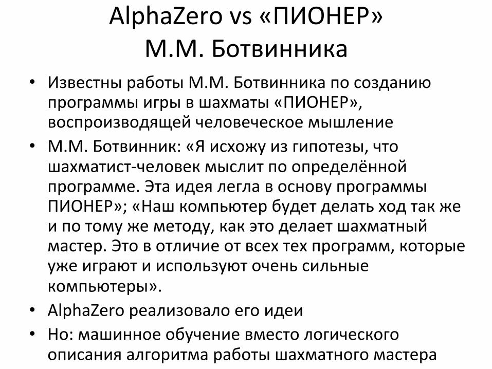
•  Известны работы М.М. Ботвинника по созданию программы игры в шахматы «ПИОНЕР», воспроизводящей человеческое мышление

•  М.М. Ботвинник: «Я исхожу из гипотезы, что шахматист-‐человек мыслит по определённой программе. Эта идея легла в основу программы ПИОНЕР»; «Наш компьютер будет делать ход так же и по тому же методу, как это делает шахматный мастер. Это в отличие от всех тех программ, которые уже играют и используют очень сильные компьютеры».

•  AlphaZero реализовало его идеи •  Но: машинное обучение вместо логического описания алгоритма работы шахматного мастера

Что дальше? •  Человек обучается на много меньшем числе игр

•  Можно ли эти технологии перенести за пределы игр, «в реальный мир»?

•  Достоинство AlphaGo: алгоритмы довольно общие, особенности игры го почти не используются

•  Объявлено об изучении сворачивания белка с потенциальными применениями в фармакологии

Заключение

Новизна подхода AlphaGo и AlphaZero заключается в совмещении 1)  методов машинного обучение (нейронных

сети глубокого обучения) и 2)  традиционных методов информатики

(метода Монте-‐Карло для поиска на дереве).

1 0 -1

1 0 -1

1 0 -1

Convolve with Threshold

Convolutional Neural Network

Input Layer

Output Layer

slide by Abi-Roozgard

Свёрточные нейронные сети

Фильтр: вычленение элементов

1 0 -1

1 0 -1

1 0 -1

Convolve with Threshold

Convolutional Neural Network

Input Layer

Output Layer

slide by Abi-Roozgard

Свёрточные нейронные сети

Многослойная сеть: выход одного слоя – вход следующего Обучение – подбор Коэффициентов wkl и b для каждого фильтра и слоя

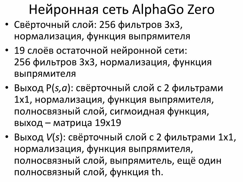
Нейронная сеть AlphaGo Zero •  Свёрточный слой: 256 фильтров 3х3, нормализация, функция выпрямителя

•  19 слоёв остаточной нейронной сети: 256 фильтров 3х3, нормализация, функция выпрямителя

•  Выход P(s,a): свёрточный слой с 2 фильтрами 1х1, нормализация, функция выпрямителя, полносвязный слой, сигмоидная функция, выход – матрица 19х19

•  Выход V(s): свёрточный слой с 2 фильтрами 1х1, нормализация, функция выпрямителя, полносвязный слой, выпрямитель, ещё один полносвязный слой, функция th.

Компьютерные,шахматы ... · Go AlphaZero AG0 3-day 31 – 19 AG0 3-day AlphaZero...

Documents

Transcript of Компьютерные,шахматы ... · Go AlphaZero AG0 3-day 31 – 19 AG0 3-day AlphaZero...