Oded Maler - NYU Computer Science
31
Continuous Systems Verification Oded Maler CNRS - VERIMAG Grenoble, France Amir Pnueli Memorial Symposium 2010
Transcript of Oded Maler - NYU Computer Science

Continuous Systems Verification
Oded Maler
CNRS - VERIMAGGrenoble, France
Amir Pnueli Memorial Symposium 2010

Introduction
I According to Manna and Pnueli, a verification framework hasthree ingredients:
I A system model: a formalism for describing the designedsystem (automata, transition systems, programs)
I A specification language: a formalism for describing thedesired properties of the system. In other words a criterion forclassifying event sequences as good or bad
I A verification technique: a method to show that (some/all)behaviors generated by the system are acceptable according tothe specification

Introduction
I In this talk we focus on:I System models which are continuous dynamical systems
defined by differential equations,I algorithmic verification against simple properties
I Initial motivation: real-time, embedded, cyber-physical andother buzzwordful systems where computers control aphysical environment
I Additional collected motivations: new techniques in appliedmathematics, verification of analog circuits, analyzingbiochemical reactions
I We use the latter domain for motivation but the concepts andalgorithms are rather generic

Summary
I We propose a computer-aided methodology to help analyzingcertain biological models
I Domain of applicability: biochemical reactions modeled asdifferential equations
I State variables denote concentrations
I We propose reachability computation, a kind of set-basedsimulation, that may replace uncountably-many simulations
I The continuous analogue of algorithmic verification(model-checking), emerged from more than a decade ofresearch on hybrid systems

Outline
I Under-determined dynamical models and their biologicalrelevance
I Continuous dynamical systems and abstract reahcability
I Effective representation of sets and concrete algorithms forlinear systems
I Treating nonlinear systems via hybridization
I Dynamic hybridization: idea and preliminary results
I Conclusions
I Appendix

Dynamical Models with Nondeterminism
I Dynamical system: state space X and a rule x ′ = f (x , v)
I The next state is a function of the current state and someexternal influence (or unknown parameters) v ∈ V
I In discrete domains: a transition system with input (alphabet)
I System becomes nondeterministic if input is projected away
I Given initial state, many possible evolutions (“runs”)
I Simulation: picking one input and generating one behavior
I Symbolic verification: magically computing all runs inparallel
I Reachability computation: adapting these ideas to systemsdefined by differential equations or hybrid automata(differential equations with mode switching)

Why Bother?
I Differential models of biochemical reactions are very imprecisefor many reasons:
I They are obtained by measuring populations, not individuals
I Kinetic parameters are based on isolated experiments notalways under same conditions
I Etc.
I It is nice to match an experimentally-observed behavior by adeterministic model, but can we do better?
I After all, biological systems are supposed to be robust undervariations in environmental conditions and parameters
I Showing that all trajectories corresponding to a range ofparameters and external disturbances exhibit the samequalitative behavior is a much stronger potentialcontribution

Preliminary Definitions and Notations
I A time domain T = R+, state space X ⊆ Rn, input spaceV ⊆ Rm
I Trajectory: partial function ξ : T → X , Input signal:ζ : T → V both defined over an interval [0, r ] ⊂ T
I A continuous dynamical system S = (X ,V , f )
I Trajectory ξ with endpoints x and x ′ is the response of S toinput signal ζ if
I ξ is the solution of x = f (x , v) for initial condition x and
v(·) = ζ, denoted by xζ/ξ−→ x ′
I R(x , ζ, t) = {x ′} denote the fact that x ′ is reachable from x
by ζ within t time, that is, xζ/ξ−→ x ′ and |ζ| = |ξ| = t
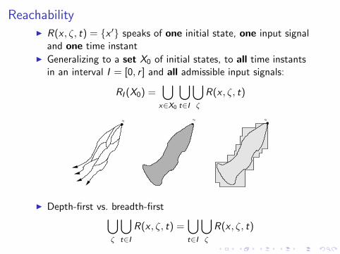
ReachabilityI R(x , ζ, t) = {x ′} speaks of one initial state, one input signal
and one time instantI Generalizing to a set X0 of initial states, to all time instants
in an interval I = [0, r ] and all admissible input signals:
RI (X0) =⋃
x∈X0
⋃t∈I
⋃ζ
R(x , ζ, t)
x0x0x0
I Depth-first vs. breadth-first⋃ζ
⋃t∈I
R(x , ζ, t) =⋃t∈I
⋃ζ
R(x , ζ, t)
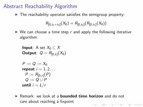
Abstract Reachability Algorithm
I The reachability operator satisfies the semigroup property:
R[0,t1+t2](X0) = R[0,t2](R[0,t1](X0))
I We can choose a time step r and apply the following iterativealgorithm:
Input: A set X0 ⊂ XOutput: Q = R[0,L](X0)
P := Q := X0
repeat i = 1, 2 . . .P := R[0,r ](P)Q := Q ∪ P
until i = L/r
I Remark: we look at a bounded time horizon and do notcare about reaching a fixpoint

From Abstract to Concrete Algorithms
I The algorithm performs operations on subsets of Rn which,mathematically speaking, can be weird objects
I Like any computational geometry we restrict ourselves toclasses of subsets (boxes, polytopes, ellipsoids, zonotopes)having nice properties:
I Finite syntactic representation
I Effective decision procedure for membership
I Closure (or approximate closure) under the reachabilityoperator
I In this talk we use convex polytopes and their finite unions

Convex Polytopes
I Halfspace: all points x satisfying a linear inequality a · x ≤ b
I Convex polyhedron: intersection of finitely many halfspaces;Polytope: bounded convex polyhedron
I Convex combination of a set of points {x1, . . . , xl} is anyx = λ1x1 + · · ·+ λlxl such that
∑li=1 λi = 1
I The convex hull conv(P) of a set P of points is the set of allconvex combinations of elements in P
I Polytope representations:I Vertices: a polytope P admits a finite minimal set P
(vertices) such that P = conv(P).I Inequalities: a polytope P admits a canonical set of
halfspaces/inequalities such that P =∧k
i=1 ai · x ≤ bi

Autonomous (Closed, Deterministic) Linear Systems
I Systems defined by linear differential equations of the formx = Ax for a matrix A are the most well-studied
I There is a standard technique to fix a time step r and work indiscrete time, a recurrence equation of the form xi+1 = Axi
I The image of a set P by the linear transformation A isAP = {Ax : x ∈ P} (one-step successors)
I It is easy to compute, for example, for polytopes representedby vertices:P = conv({x1, . . . , xl}) ⇒ AP = conv({Ax1, . . . ,Axl})
v1
v2
v4
v5
v6
v3
P
v ′4 = Av4
v ′5 = Av5
v ′6 = Av6
v ′1 = Av1
AP
v ′3 = Av3
v ′2 = Av2

Algorithm 1: Discrete-Time Linear Reachability
I Input: A set X0 ⊂ X represented as conv(P0)
I Output: Q = R[0..L](X0) represented as a list
{conv(P0), . . . , conv(PL)}
P := Q := P0
repeat i = 1, 2 . . .P := APQ := Q ∪ P
until i = L
I Assuming |P0| = m0, the complexity of the algorithm isO(m0LM(n)) where M(n) is the complexity of matrix-vectormultiplication in n dimensions: ∼ O(n3)
I Can be applied to other representations of objects closedunder linear transformations

Linear Systems with Input (Minkowski Sum Approach)
I Systems define by xi+1 = Axi + vi where the vi ’s range over abounded convex set V
I The one-step successor of P is defined as
P ′ = {Ax + v : x ∈ P, v ∈ V } = AP ⊕ V
I Minkowski sum A⊕ B = {a + b : a ∈ A ∧ b ∈ b}I Same algorithm can be applied but the Minkowski sum
increases the number of vertices/facets in every step
P ⊕ V
P
V

Alternative: Face Lifting
I Over-approximating the reachable set while keeping itscomplexity more or less fixed
I Assume P represented as intersection of halfspaces
I For each halfspace H i : aix ≤ bi , let v i ∈ V be the inputvector which pushes it in the “outermost” way
I Apply Ax + Bv i to H i and the intersection of the pushedhalfspaces over-approximates AP ⊕ V
P ′ ⊃ P ⊕ V
PV
I The enemy of the people is the wrapping effect:over-approximation errors accumulate every step
Linear State of the Art (Minkowski Approach)
I New algorithmics by C. Le Guernic and A. Girard
I Efficient computations: linear transformation applied to afixed number of points in each iteration
I No accumulation of over-approximation errors
I Initially used zonotopes, a class of sets closed under bothlinear operations and Minkowski sum; Can be applied to any“lazy” representation of the sequence of the computed sets
I Based on the observation that two consecutive sets
Pk = AkP0 ⊕ Ak−1V ⊕ Ak−2V ⊕ . . .⊕ VPk+1 = Ak+1P0 ⊕ AkV ⊕ Ak−1V ⊕ . . .⊕ V
share a lot of terms
I Can compute within few minutes 1000 reachability steps forlinear systems with 200 (!) state variables

Linear State of the Art (Optimization Approach)
I Recent result by T. Dang and R. Testylier
I Observation: over-approximation error on sharp corners canbe significantly reduced by adding redundant constraints
I Moreover, the extra constraint can be added in the rightplace and orientation, after the over-approximating setintersects the bad set
I A kind of dynamic approximation refinementI No need to move between constraint and vertex
representations
I A prototype can easily handle 100 dimensions

Linear Reachability: Some Credits
I Algorithmic analysis of hybrid systems started with tools likeKronos and HyTech for timed automata and “linear” hybridautomata: HenzingerSifakisYovine,HenzingerHoWongtoi
I Very simple continuous dynamics, summarized in ACH+95
I Verifying differential equations: Greenstreet96
I Reachability for linear differential equations and hybridsystems: ChutinanKrogh99, AsarinBournezDangMaler00(polytopes) KurzhanskiVaraiya00, BotchkarevTripakis00(ellipsoids), MitchellTomlin00 (level sets)
I Pushing faces and treating inputs: DangMaler98, Varaiya98
I Using zonotopes: Girard05
I New algorithmic schemes LeGuernic Girard06-09,DangTestylier10

The Nonlinear Challenge
I Ok, bravo, but linear systems were studied to death byeverybody
I Real interesting models, biological included, are nonlinear
I What about systems of the form xi+1 = f (xi , ui ) or evensimply xi+1 = f (xi ) where f is an arbitrary continuousfunction, say a polynomial ?
I Nonlinear maps do not preserve convexity
I You can make small time steps, use a local linearapproximation and bloat the obtained set to be safe
I This approach will either accumulate large errors or requirevery expensive computation in every step of the main loop
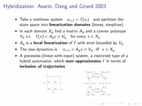
Hybridization: Asarin, Dang and Girard 2003
I Take a nonlinear system xi+1 = f (xi ) and partition thestate space into linearization domains (boxes, simplices)
I In each domain Xq find a matrix Aq and a convex polytopeVq s.t. f (x) ∈ Aqx ⊕ Vq for every x ∈ Xq
I Aq is a local linearization of f with error bounded by Vq
I The new dynamics is xi+1 ∈ Aqx ⊕ Vq iff x ∈ Xq
I A piecewise-(linear-with-input) system, a restricted type of ahybrid automaton, which over-approximates f in terms ofinclusion of trajectories
10
1101
00
x2 ≥ d2x2 ≤ d2x2 ≤ d2
x1 ≥ d1
x1 ≤ d1
x1 ≥ d1
x1 ≤ d1
x ∈ A00 · x ⊕ V00 x ∈ A10 · x ⊕ V10
x ∈ A01 · x ⊕ V01 x ∈ A11 · x ⊕ V11
x2 ≥ d2
d1
x1X10X00
X01 X11d2
x2

Hybridization (cont.)
10
1101
00
x2 ≥ d2x2 ≤ d2x2 ≤ d2
x1 ≥ d1
x1 ≤ d1
x1 ≥ d1
x1 ≤ d1
x ∈ A00 · x ⊕ V00 x ∈ A10 · x ⊕ V10
x ∈ A01 · x ⊕ V01 x ∈ A11 · x ⊕ V11
x2 ≥ d2
d1
x1X10X00
X01 X11d2
x2
I In the hybrid automaton, x evolves according to the lineardynamics Aqx ⊕ Vq as long as it remains in Xq
I Reaching the boundary between Xq and Xq′ , it takes atransition to q′ and evolves according to Aq′x ⊕ Vq′
I Linearization and error are recomputed only while crossingdomain boundaries, not in every step
I Approximation quality can be tuned by controlling the size oflinearization domains

Hybrid Reachability
10
1101
00
x2 ≥ d2x2 ≤ d2x2 ≤ d2
x1 ≥ d1
x1 ≤ d1
x1 ≥ d1
x1 ≤ d1
x ∈ A00 · x ⊕ V00 x ∈ A10 · x ⊕ V10
x ∈ A01 · x ⊕ V01 x ∈ A11 · x ⊕ V11
x2 ≥ d2
d1
x1X10X00
X01 X11d2
x2
I Compute in one domain a sequences of sets using lineartechniques until a set intersects with a boundary
I Take the intersection as initial set in the next domain andapply linear reachability with the corresponding linearization
(a) (b)
A1 A2

Between Theory and Practice
I First problem: intersection may be spread over many steps:
(c)(b)(a)
I Either explosion or union of intersections, error accumulation
I Major problem: a set may leave a box via many facets:
(a) (b)
I Consequently, static hybridization is practically impossiblebeyond 3 dimensions
I Set splitting is an artifact of the fixed grid that we violentlyimposed on Space

The Solution: Dynamic Hybridization
I A dynamic hybridization scheme not based on a fixed grid
I In this scheme we do not need intersection at all and weallow the linearization domains to overlap
I When we leave a domain, we backtrack one step and define anew linearization domain around the previous set andcontinue with the new linearized dynamics from there
PiPi
P0P0
B
(a)
B
(b)
B′
I And it works!

Example: E. Coli Lac Operon
Ra = τ − µ ∗ Ra − k2RaOf + k−2(χ− Of )− k3RaI2i + k8RiG
2
Of = −k2raOf + k−2(χ− Of )
E = νk4Of − k7E
M = νk4Of − k6M
Ii = −2k3RaI2i + 2k−3F1 + k5IrM − k−5IiM − k9IiE
G = −2k8RiG2 + 2k−8Ra + k9IiE
I We can also do a 9-dim highly-nonlinear aging model, and amodel of an angiogenesis pathway (14-dim polynomial DE)

Conclusions
I Disclaimer: we do not bring any new biological insight onany concrete system at this point
I Our goal is to develop tools, as general-purpose as possible,that can aid in the analysis of many non-trivial systems
I Problem specificity cannot be avoided of course: it willcome up at the particular modeling and exploration phases
I Methodological aspects of the use of such tools in thebiological context should be worked out
I Work in progress: optimizing the choice of size andorientation of the linearizarization domains
I Current version is still a prototype, based on the oldalgorithmics for linear systems, hence we are optimistic aboutgoing to even higher dimensions

Commercial I: SpaceEx
I Coming soon: SpaceEx the state space explorer (G. Frehse)
I A tool platform for developing hybrid verification tools
I Two tools will be released in 2010: PHAVer 2.0 for linearhybrid automata and a tool for piecewise-lineardifferential equations using support function representation
I Web interface

And What About Temporal Logic?
I The logic STL (signal temporal logic), an extension of thereal-time logic MITL with numerical predicates
I Example: a water-level controller for a nuclear plant shouldmaintain a controlled variable y around a fixed level despiteexternal disturbances x
I We want y to stay always in the interval [−30, 30] except,possibly, for an initialization period of duration 300
I If, due to disturbances, y goes outside the interval [−0.5, 0.5],it should return to it within 150 time units and stay there forat least 20 time units
I The property is expressed as
�[300,2500]((|y | ≤ 30)∧((|y | > 0.5)⇒ ♦[0,150]�[0,20](|y | ≤ 0.5)))

Commercial II: AMT
I The Analog Monitoring Tool (D. Nickovic) is available fordownload

Thank You