spe 492-34 1st pgs page 1

1

The Geological Society of AmericaSpecial Paper 492

2012

Oceanography and Google Earth: Observing ocean processes with time animations and student-built ocean drifters

Alfred Hochstaedter*Earth Science Department, Monterey Peninsula College, 980 Fremont Street, Monterey, California 93940, USA

Deidre SullivanMarine Advanced Technology Education (MATE) Center, Monterey Peninsula College, 980 Fremont Street,

Monterey, California 93940, USA

ABSTRACT

Google Earth provides an easily accessible platform for students to view anima-tions of oceanographic processes created by merging satellite, buoy, and student-built ocean-drifter data. The power of Google Earth is that many oceanographic proper-ties can be displayed simultaneously over time such as atmospheric pressure, winds, surface currents, and sea-surface temperature. Lessons created from these activities address many of the principal outcomes of an introductory oceanography course, including the ability to analyze the interrelationship of ocean processes and under-stand how modern oceanography relies on technology to observe and measure the state of the oceans. In the classroom, the time-animation effort is paired with a drifter project where students build and release Global Positioning System–equipped drift-ers and watch their movement via satellite over the Internet. Because students see, touch, and feel the drifter in the classroom as they build and decorate it, they develop an inherent interest in its fate. Following the movement of the drifter fosters student interest in related oceanographic processes, many of which can be animated in Google Earth for the same time period, providing easy comparisons. The satellite data used in these animations are accessed through the National Oceanic and Atmospheric Admin-istration (NOAA) Southwest Fisheries Science Center’s ERDDAP (Environmental Research Division’s Data Access Program) data server and displayed in Google Earth using keyhole markup language (KML) scripts. Satellite products are downloaded as .png image fi les and displayed as a series of image overlays to create time animations. Python scripts automate the process of generating KML scripts.

*ahochstaedter@mpc.edu

Hochstaedter, A., and Sullivan, D., 2012, Oceanography and Google Earth: Observing ocean processes with time animations and student-built ocean drifters, in Whitmeyer, S.J., Bailey, J.E., De Paor, D.G., and Ornduff, T., eds., Google Earth and Virtual Visualizations in Geoscience Education and Research: Geological Society of America Special Paper 492, p. 1–XXX, doi:10.1130/2012.2492(34). For permission to copy, contact editing@geosociety.org. © 2012 The Geological Society of America. All rights reserved.

2 Hochstaedter and Sullivan

spe 492-34 1st pgs page 2

INTRODUCTION

Oceanography Today

Studying earth systems and how they are interconnected has become a central theme in science starting in the 1970s with the Gaia hypothesis (Lovelock, 1979). The earth system is so inter-connected that being able to fully understand and predict any part of it depends on integrating measurements and observations from many disciplines over a wide range of spatial and tempo-ral scales (Rayner, 2010). Twenty-fi rst century oceanography, as with many fi elds in science, has migrated from that of discrete sampling (such as observations made from a ship at a particu-lar time and place) to continuous sampling made from fl oating buoys, autonomous underwater vehicles, and cabled underwa-ter observatories augmented with remotely sensed data from satellites (Spinrad, 2006; Lubchenco, 2010). Ocean observing systems such as the U.S. Integrated Ocean Observing System (IOOS) and the international Global Ocean Observing System (GOOS) are coming of age to understand ocean processes and address issues of global concern just as accurate weather fore-casts are dependent upon globally integrated measurements and observations of the atmosphere and oceans delivered on a con-sistent and timely basis.

The realization that it is the interconnection of earth system processes that is the dominant theme, and that these processes constantly undergo changes spatially and on seasonal, yearly, and decadal timescales, has prompted a shift in the way the oceans are studied, described, taught, and ultimately perceived.

Monitoring programs, such as IOOS and GOOS, have produced enormous quantities of data, much of which is avail-able for public download over the Internet. Like never before, students, as well as the general public, are able to access and evaluate the data used to support or argue against scientifi c ideas as well as policy decisions, such as the placement of marine pro-tected areas, climate change policy, oil-spill mitigation and fi sh-ing regulations. In addition, students can use these data to test hypotheses or make predictions during their own inquiry-based learning experiences. There are so many sources of large quanti-ties of data that new organizations have been developed to coor-dinate and encourage the dissemination of these new sources of information. IOOS has been referred to as a “social network of organizations and people” that fosters the effi cient and effective connection of ocean data and information to a large network of interested parties (U.S. IOOS Offi ce, 2010).

The changes under way in the ocean sciences are represen-tative of changes occurring in nearly every branch of science and technology. The ability to visualize complex interactions is a requirement across the science, technology, engineering, and mathematics (STEM) fi elds from earth sciences to materials sciences to engineering. In all of these fi elds, workplace skills require new employees to be able to fi nd relevant information and data, acquire it many times via download, manipulate it, and visualize it in useful and fl exible ways. The ability to investigate

ocean processes using real-time data is becoming an essential skill in today’s workplace.

Challenges that impair these efforts include the diffi culty of downloading data from a wide variety of Internet portals and the lack of visceral experience that students have with important oceanographic properties such as atmospheric pressure, nutrient concentrations, or changes in sea-surface temperature. Although much data are readily available, the methods to download and the formats of the downloaded data are extremely variable. For many students, just downloading the data and seeing it in the right for-mat becomes the primary task rather than learning something from the data itself.

The Opportunity—Student-Built Drifters and Visualizations using Google Earth Time Animations

To address these challenges the Marine Advanced Technol-ogy Education (MATE) Center has developed a two-pronged approach designed for introductory oceanography courses. Many of these students lack a tangible understanding of the scientifi c process, or previous experiences with ocean currents or changes in ocean properties over time or space. For many students, ocean-ography will be their only collegiate-level science course.

First, in an effort to give students direct exposure to ocean technology that enables much of modern oceanography, we have the students participate in the construction of relatively simple, ocean drifters equipped with Global Positioning System (GPS) transponders (i.e., two-way communications that can send and receive geographic position information). Once deployed, stu-dents can watch the movement of the drifter in real-time over the Internet. The notion of students watching the motion of an object that they helped build, decorate, and launch that is now in the ocean, helps spur interest in additional ocean characteristics that are changing on the same timescales that the drifter is observing.

The second part to our approach is downloading oceano-graphic data—sea-surface temperature, chlorophyll, sea-surface height, winds, and atmospheric pressure collected from satellites and oceanic buoys—and then displaying them in Google Earth for the same temporal and geographic extent as the drifter in the water. Google Earth lends itself to these tasks because of its familiarity to students, ease of use, and ability to create anima-tions of changes over time.

The MATE ocean drifter project enables students to be involved in the collection of oceanographic data that is also of interest to local scientists. Through collaborations with research institutions, government agencies, and non-profi t organiza-tions, students can feel a part of an ongoing scientifi c study and instructors can reap the benefi ts of collaboration with science colleagues. Such collaborations enable the instructors, teachers, and educators to more fully understand the science behind the scientifi c study. These drifters have been deployed by colleges and universities to help support studies addressing: harmful algal blooms; the transport of fi sh, clam, lobster, and crab larvae; the movement of oil during the Deep Horizon spill; the movement of

Oceanography and Google Earth 3

spe 492-34 1st pgs page 3

trash in rivers during fl ood stage; currents for tidal power; the dis-persion of power plant effl uent; and surface circulation and circu-lation model validation. These efforts often inspire the instructor to be more enthusiastic and share their passion for science with the students.

The Impact

In this paper, we describe our efforts in building drifters, equipping them with GPS transponders, following their move-ment over the Internet, and creating Keyhole Markup Lan-guage (KML) scripts to display associated oceanographic data in Google Earth in animated formats. The result of these efforts is an effective method to teach the science of complex ocean systems. Students see data rather than generalized textbook dia-grams and gain an appreciation of the complexity and variability of ocean processes from the experience. These efforts emphasize the reliance of modern ocean science on technology and open the doors of opportunity for collaboration between ocean scientists and educators.

STUDENT-BUILT DRIFTERS

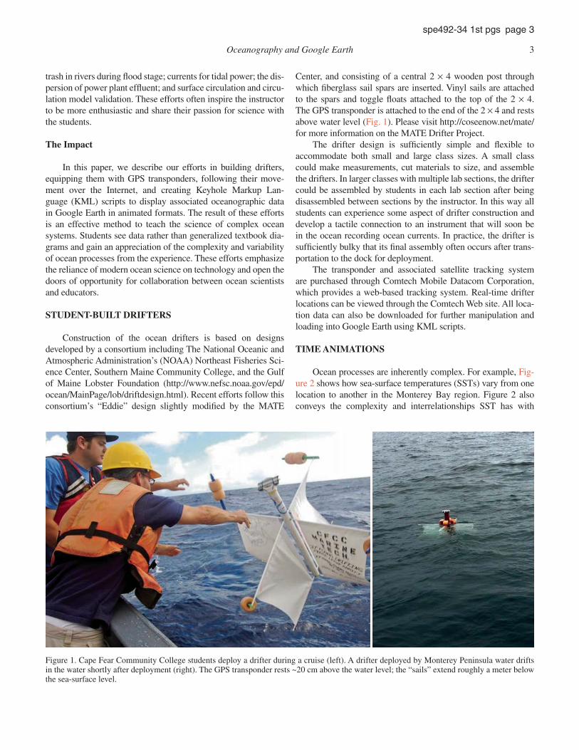
Construction of the ocean drifters is based on designs developed by a consortium including The National Oceanic and Atmospheric Administration’s (NOAA) Northeast Fisheries Sci-ence Center, Southern Maine Community College, and the Gulf of Maine Lobster Foundation (http://www.nefsc.noaa.gov/epd/ocean/MainPage/lob/driftdesign.html). Recent efforts follow this consortium’s “Eddie” design slightly modifi ed by the MATE

Center, and consisting of a central 2 × 4 wooden post through which fi berglass sail spars are inserted. Vinyl sails are attached to the spars and toggle fl oats attached to the top of the 2 × 4. The GPS transponder is attached to the end of the 2 × 4 and rests above water level (Fig. 1). Please visit http://coseenow.net/mate/ for more information on the MATE Drifter Project.

The drifter design is suffi ciently simple and fl exible to accommodate both small and large class sizes. A small class could make measurements, cut materials to size, and assemble the drifters. In larger classes with multiple lab sections, the drifter could be assembled by students in each lab section after being disassembled between sections by the instructor. In this way all students can experience some aspect of drifter construction and develop a tactile connection to an instrument that will soon be in the ocean recording ocean currents. In practice, the drifter is suffi ciently bulky that its fi nal assembly often occurs after trans-portation to the dock for deployment.

The transponder and associated satellite tracking system are purchased through Comtech Mobile Datacom Corporation, which provides a web-based tracking system. Real-time drifter locations can be viewed through the Comtech Web site. All loca-tion data can also be downloaded for further manipulation and loading into Google Earth using KML scripts.

TIME ANIMATIONS

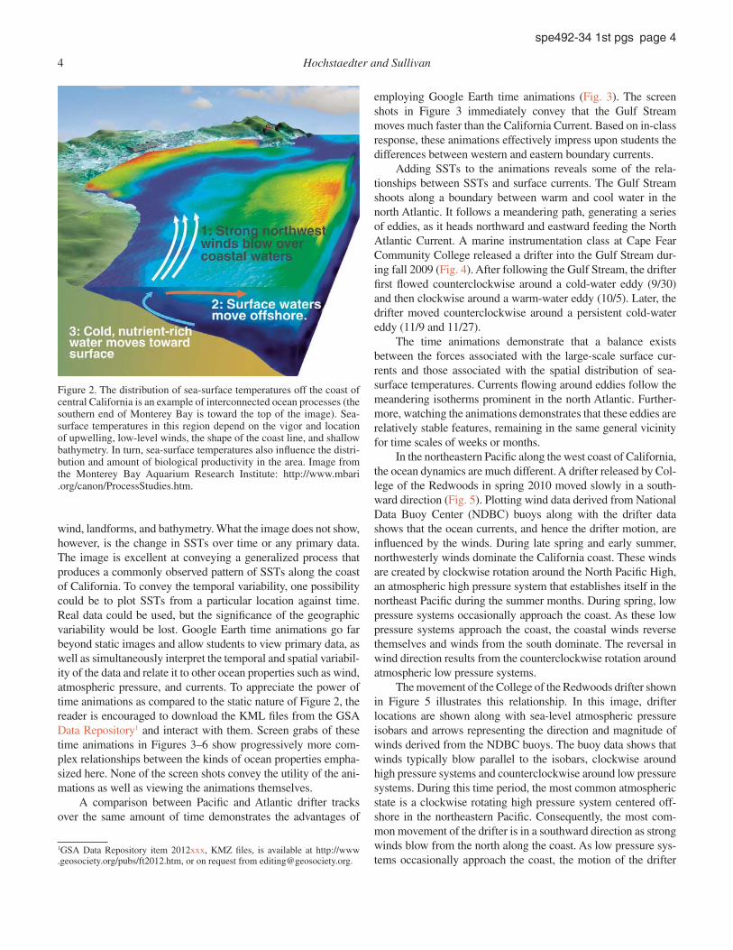
Ocean processes are inherently complex. For example, Fig-ure 2 shows how sea-surface temperatures (SSTs) vary from one location to another in the Monterey Bay region. Figure 2 also conveys the complexity and interrelationships SST has with

Figure 1. Cape Fear Community College students deploy a drifter during a cruise (left). A drifter deployed by Monterey Peninsula water drifts in the water shortly after deployment (right). The GPS transponder rests ~20 cm above the water level; the “sails” extend roughly a meter below the sea-surface level.

4 Hochstaedter and Sullivan

spe 492-34 1st pgs page 4

wind, landforms, and bathymetry. What the image does not show, however, is the change in SSTs over time or any primary data. The image is excellent at conveying a generalized process that produces a commonly observed pattern of SSTs along the coast of California. To convey the temporal variability, one possibility could be to plot SSTs from a particular location against time. Real data could be used, but the signifi cance of the geographic variability would be lost. Google Earth time animations go far beyond static images and allow students to view primary data, as well as simultaneously interpret the temporal and spatial variabil-ity of the data and relate it to other ocean properties such as wind, atmospheric pressure, and currents. To appreciate the power of time animations as compared to the static nature of Figure 2, the reader is encouraged to download the KML fi les from the GSA Data Repository1 and interact with them. Screen grabs of these time animations in Figures 3–6 show progressively more com-plex relationships between the kinds of ocean properties empha-sized here. None of the screen shots convey the utility of the ani-mations as well as viewing the animations themselves.

A comparison between Pacifi c and Atlantic drifter tracks over the same amount of time demonstrates the advantages of

Figure 2. The distribution of sea-surface temperatures off the coast of central California is an example of interconnected ocean processes (the southern end of Monterey Bay is toward the top of the image). Sea-surface temperatures in this region depend on the vigor and location of upwelling, low-level winds, the shape of the coast line, and shallow bathymetry. In turn, sea-surface temperatures also infl uence the distri-bution and amount of biological productivity in the area. Image from the Monterey Bay Aquarium Research Institute: http://www.mbari.org/canon/ProcessStudies.htm.

employing Google Earth time animations (Fig. 3). The screen shots in Figure 3 immediately convey that the Gulf Stream moves much faster than the California Current. Based on in-class response, these animations effectively impress upon students the differences between western and eastern boundary currents.

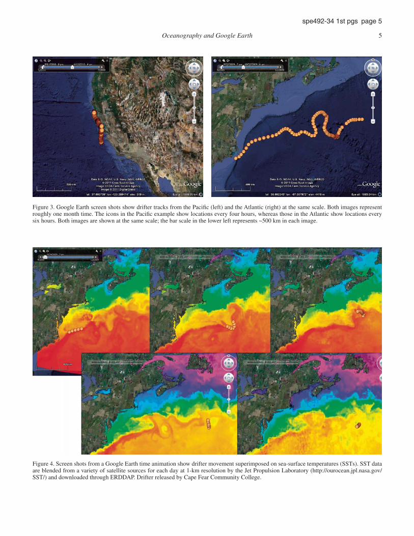
Adding SSTs to the animations reveals some of the rela-tionships between SSTs and surface currents. The Gulf Stream shoots along a boundary between warm and cool water in the north Atlantic. It follows a meandering path, generating a series of eddies, as it heads northward and eastward feeding the North Atlantic Current. A marine instrumentation class at Cape Fear Community College released a drifter into the Gulf Stream dur-ing fall 2009 (Fig. 4). After following the Gulf Stream, the drifter fi rst fl owed counterclockwise around a cold-water eddy (9/30) and then clockwise around a warm-water eddy (10/5). Later, the drifter moved counterclockwise around a persistent cold-water eddy (11/9 and 11/27).

The time animations demonstrate that a balance exists between the forces associated with the large-scale surface cur-rents and those associated with the spatial distribution of sea-surface temperatures. Currents fl owing around eddies follow the meandering isotherms prominent in the north Atlantic. Further-more, watching the animations demonstrates that these eddies are relatively stable features, remaining in the same general vicinity for time scales of weeks or months.

In the northeastern Pacifi c along the west coast of California, the ocean dynamics are much different. A drifter released by Col-lege of the Redwoods in spring 2010 moved slowly in a south-ward direction (Fig. 5). Plotting wind data derived from National Data Buoy Center (NDBC) buoys along with the drifter data shows that the ocean currents, and hence the drifter motion, are infl uenced by the winds. During late spring and early summer, northwesterly winds dominate the California coast. These winds are created by clockwise rotation around the North Pacifi c High, an atmospheric high pressure system that establishes itself in the northeast Pacifi c during the summer months. During spring, low pressure systems occasionally approach the coast. As these low pressure systems approach the coast, the coastal winds reverse themselves and winds from the south dominate. The reversal in wind direction results from the counterclockwise rotation around atmospheric low pressure systems.

The movement of the College of the Redwoods drifter shown in Figure 5 illustrates this relationship. In this image, drifter locations are shown along with sea-level atmospheric pressure isobars and arrows representing the direction and magnitude of winds derived from the NDBC buoys. The buoy data shows that winds typically blow parallel to the isobars, clockwise around high pressure systems and counterclockwise around low pressure systems. During this time period, the most common atmospheric state is a clockwise rotating high pressure system centered off-shore in the northeastern Pacifi c. Consequently, the most com-mon movement of the drifter is in a southward direction as strong winds blow from the north along the coast. As low pressure sys-tems occasionally approach the coast, the motion of the drifter

1GSA Data Repository item 2012xxx, KMZ fi les, is available at http://www.geosociety.org/pubs/ft2012.htm, or on request from editing@geosociety.org.

Oceanography and Google Earth 5

spe 492-34 1st pgs page 5

Figure 3. Google Earth screen shots show drifter tracks from the Pacifi c (left) and the Atlantic (right) at the same scale. Both images represent roughly one month time. The icons in the Pacifi c example show locations every four hours, whereas those in the Atlantic show locations every six hours. Both images are shown at the same scale; the bar scale in the lower left represents ~500 km in each image.

Figure 4. Screen shots from a Google Earth time animation show drifter movement superimposed on sea-surface temperatures (SSTs). SST data are blended from a variety of satellite sources for each day at 1-km resolution by the Jet Propulsion Laboratory (http://ourocean.jpl.nasa.gov/SST/) and downloaded through ERDDAP. Drifter released by Cape Fear Community College.

6 Hochstaedter and Sullivan

spe 492-34 1st pgs page 6

Oceanography and Google Earth 7

spe 492-34 1st pgs page 7

slows dramatically or even reverses, moving slowly toward the north. As the low pressure system exits and high pressure once again dominates the region offshore California, the drifter contin-ues its southward movement.

Spring conditions in the northeast Pacifi c offshore of Cali-fornia are characterized by coastal upwelling. This process is shown schematically in Figure 2, and with satellite- and buoy-derived data in Figure 6. Three different parameters are shown in Figure 6: isobars of atmospheric pressure at sea-level, wind direction and magnitude at three NDBC buoys, and SSTs. Whereas the screen shot shown in Figure 6 is a snapshot in time, the time animation available in the GSA Data Repository [see footnote 1] shows how all of these parameters continuously change with time. During the North American spring and sum-mer, clockwise rotation around the high pressure system in the northeastern Pacifi c results in winds from the northwest along

Figure 5. A series of Google Earth screen shots show the relationship between atmospheric pressure (colored isobars), wind direction and magnitude (colored arrows), and drifter motion (circular icons, with most recent location on top). In A and C, high-pressure systems are most prominent off of the California coast. Air rotating clockwise around the high-pressure systems caused wind to blow from northwest to southeast during these time periods. As a result, the drifter moved with ocean currents in a southeastward direction. In B, a low-pressure system entered the region off of the California coast. Counterclock-wise fl ow around the low-pressure system caused a wind relaxation event in which winds blew weakly from south to north. As a result, the drifter stopped moving in a southeastward direction and remained relatively stationary during this time period.

the coast of North America. At any particular point in time, loca-tions where the isobars are closer together, the pressure gradient force is greater, resulting in stronger winds (compare the wind arrows off the coast of California to those off of the Columbia River in Fig. 6). Surface waters respond to the northwest winds as well as the Coriolis effect. The resulting Ekman transport causes near-surface water to fl ow in an off-shore direction. Upwelling is the replacement of this warmer near-surface water by colder, and more nutrient-rich, deep water. Upwelling causes the colder water to appear at the surface near the coast, as seen in Figure 6.

DOWNLOADING OCEANOGRAPHIC DATA FOR THE TIME ANIMATIONS

Most of the oceanographic data used in the animations shown here is downloaded from the ERDDAP (Environmental Research Division’s Data Access Program) data server main-tained by NOAA’s Southwest Fisheries Science Center (http://coastwatch.pfeg.noaa.gov/erddap/index.html). ERDDAP allows the user to specify the format of the downloaded data, as well as both the temporal and geographic extent of the downloaded data. The ERDDAP server re-serves data from a large variety of sources, including a variety of satellite products and the NDBC buoys. Currently hundreds of different data sets are available.

A key aspect of the ERDDAP portal is that data is retrievable in a variety of formats, making it easy to load into Google Earth. These formats include transparent .png image fi les which can be “draped” over the topography or sea surface as image overlays, and ASCII (American Standard Code for Information Inter-change) grids, which can be manipulated further and displayed as

Figure 6. Sea-surface temperatures (SSTs), sea-level atmospheric isobars, and wind arrows show conditions favor-able for upwelling along the California coast in June 2010. Upwelling indicated by the dark blue and purple along the central coast. In response to northwest winds created by an offshore atmo-spheric high, Ekman transport moves near-surface water away from the coast. This near-surface water is replaced by colder water from deeper levels. Thus, the cool SSTs along the coast are a re-sult of the upwelling. Drifter locations removed for clarity. This is the process shown schematically in Figure 2.

8 Hochstaedter and Sullivan

spe 492-34 1st pgs page 8

paths (polylines) or icons. Most importantly, all of the formatting variables controlling the appearance of the downloaded image (color scales, geographic boundaries, time information, etc.) are contained directly within the URL (uniform resource locator) used to download the data. This URL coding within the ERD-DAP system enables the automation of data downloading. With a predictable, systematic system of communicating the format-ting variables through the URL, simple scripts can be developed using Python, MATLAB, or similar languages, to download a series of data images, save them on a hard disk or server, and write KML scripts to load them into Google Earth in the correct chronological order, thus creating a time animation.

An easy way to download a chronologic series of data from the ERDDAP site and save the individual fi les on a local hard disk is to use the cURL utility, a command-line tool for transfer-ring data using the URL syntax (http://curl.haxx.se/). cURL is open-source software and is free to download. More information on the specifi c cURL commands to use, as well as alternative techniques, are given on ERDDAP’s documentation page (http://coastwatch.pfeg.noaa.gov/erddap/griddap/documentation.html).

CREATING KML SCRIPTS TO CONTROL THE TIME ANIMATIONS

In this section we briefl y describe portions of the KML scripts that are used to create these animations. These examples are intended to illustrate the technique and inspire new anima-tion ideas for those creating animations for beginning students or those providing instruction in KML itself to more advanced Earth and ocean science students. A full description of KML is beyond the scope of this paper. For a more detailed description of KML and descriptions of its use, see Wernecke (2009). Full KML scripts for the animations described in this paper are avail-able in the GSA Data Repository.

KML Basics

In the KML scripts, drifter locations are shown by point data, or icons. The buoy-derived wind data are also point data shown by icons. In the KML vernacular, icons, or point data, are loaded using the <Placemark> element. The yellow pushpin commonly seen in many Google Earth images is a familiar example of a <Placemark>. All of the other data, including SSTs, sea surface heights (SSHs), high-frequency radar current data, and chloro-phyll data, are shown using .png image fi les downloaded from the ERDDAP web portal. The .png image fi les are loaded using the <GroundOverlay> element. A <GroundOverlay> is an image draped over the basic satellite and seafl oor imagery native to Google Earth. The .png images are downloaded from the ERD-DAP web portal and saved to a local hard disk. The KML script then references these locally stored .png fi les.

The <Placemark> and <GroundOverlay> elements are the most important building blocks of the KML scripts that create the animations. Both <Placemark> and <GroundOverlay> are

derived from the <Feature> element, and thus contain similar child elements. This means that, like any <Feature> element, both <Placemark> and <GroundOverlay> can contain child elements that defi ne things like their <name>, <Style>, <description>, and, most importantly for animations, <TimeSpan>.

<Timespan> is a critical element in creating animations because it defi nes the dates and times for which the <Placemark> (i.e., icon) and <GroundOverlay> (i.e., .png images) should be visible to the viewer. The <Timespan> element has two child ele-ments: <begin> and <end>, each of which contain a “dateTime” value. The values contained by the <begin> and <end> elements document when to begin and end showing a <Placemark> or <GroundOverlay>.

The <TimeSpan> element has the following format:

<TimeSpan> <begin>dateTime</begin> <end>dateTime</end></TimeSpan>

The dateTime value within the <begin> and <end> elements specifi es a date ± time in UTC (Coordinated Universal Time). The dateTime has the following format:

yyyy-mm-ddThh:mm:ss

where:• yyyy is a four-digit value that specifi es the year (e.g., 2011).• mm is a two-digit value that specifi es the month between

01 and 12 (e.g., 08 for August).• dd is a two-digit value that specifi es the day of the month

between 01 and 31 (e.g., 03 for the third day of the month).• T is the separator between the date and the time.• hh is a two-digit value for hours between 00 and 24.• mm is a two-digit value for minutes between 00 and 60.• ss is a two-digit value for seconds between 00 and 60.

An SST Animation Example

An example of KML script for displaying the .png fi les fol-lows (Table 1). Each <GroundOverlay> element contains sev-eral child elements. In the order shown in the KML script, these include <name> which defi nes the name of the <GroundOver-lay> as seen in the list view on the left-hand side of the Google Earth screen, <TimeSpan> which defi nes the date and time the <GroundOverlay> is visible as described above, <Icon> which contains the child element <href> which tells Google Earth which .png fi le and the location of the fi le to associate with this particular <GroundOverlay>, and <LatLonBox> which contains child elements that defi ne location and spatial extent over which Google Earth should display the .png image fi le.

The <GroundOverlay> element is repeated for each .png fi le that needs to be displayed to create the animation. For the SST data used in these examples, a single image is produced for

Oceanography and Google Earth 9

spe 492-34 1st pgs page 9

each day. Therefore, the <TimeSpan> element describes a 24-h window for display and a different <GroundOverlay> element is inserted into the KML script for each day of the animation. Each <GroundOverlay> element contains a <name> element. The value contained within each of these <name> elements is a date—the date that the SST data was collected. Thus, this <name> element helps the viewer identify when the data shown in each .png image was collected.

A Drifter Track Example

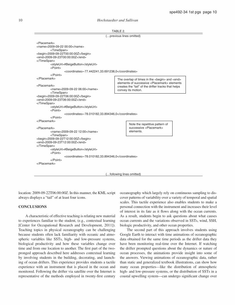
An example of a KML script for displaying drifter loca-tions as point data within a <Placemark> element follows (Table 2). Each <Placemark> element contains several child elements. As with the <GroundOverlay> element described above, these child elements include the <name> and <TimeSpan> elements which behave similarly for <Placemark>. In addition, the <Place-mark> element also contains two additional child elements. The

<styleUrl> element contains a reference to a description of the style for the icon that is defi ned elsewhere in the KML script. This style contains a reference to a .png fi le to be used as an icon, the color and size of the icon, and other attributes defi ning what the icon should look like to the Google Earth viewer. The <Point> element contains a <coordinates> element that defi nes the location to display the icon with coordinates in the order of longitude, latitude, and altitude.

The <Placemark> element is repeated for each drifter loca-tion that is part of the animation. For the drifter data used in these examples, the <TimeSpan> element is manipulated so that the drifter track always has a “tail” of a few previous drifter loca-tions. This “tail” helps the viewer’s eye visualize the motion of the drifter. This “tail” is accomplished by giving each drifter location an <end> time that is after the <begin> time of the next drifter location. For example, in the KML script shown in the box, the <end> time of the fi rst drifter location is 2009-09-23T00:00:00Z, which is 18 h after the <begin> time of the second drifter

TABLE 1.

<?xml version="1.0" encoding="UTF-8"?> <kml xmlns="http://www.opengis.net/kml/2.2" xmlns:gx="http://www.google.com/kml/ext/2.2" xmlns:kml="http://www.opengis.net/kml/2.2" xmlns:atom="http://www.w3.org/2005/Atom"> <Document> <name>EastPac SST Data and Legend</name> <Folder> <name>SST Data</name> <GroundOverlay> <name>2011-07-05 Data</name> <TimeSpan> <begin>2011-07-05T00:00:00</begin> <end>2011-07-06T00:00:00</end> </TimeSpan> <Icon> <href>C:/Folder/EastPacSST-2011-07-05.png </href> </Icon> <LatLonBox> <north>48.005 </north> <south>23.005 </south> <east>-115.995 </east> <west>-139.995 </west> </LatLonBox> </GroundOverlay> <GroundOverlay> <name>2011-07-06 Data</name> <TimeSpan> <begin>2011-07-06T00:00:00</begin> <end>2011-07-07T00:00:00</end> </TimeSpan> <Icon> <href>C:/Folder/EastPacSST-2011-07-06.png </href> </Icon> <LatLonBox> <north>48.005 </north> <south>23.005 </south> <east>-115.995 </east> <west>-139.995 </west> </LatLonBox> </GroundOverlay> (…following lines omitted)

Note relationship between the values in <name>, <begin>, <end>, and the .png file in <ref>.

End of the first <GroundOverlay> and beginning of the second <GroundOverlay>.

Note the repetitive pattern.

10 Hochstaedter and Sullivan

spe 492-34 1st pgs page 10

location: 2009-09-22T06:00:00Z. In this manner, the KML script always displays a “tail” of at least four icons.

CONCLUSIONS

A characteristic of effective teaching is relating new material to experiences familiar to the student, (e.g., contextual learning [Center for Occupational Research and Development, 2011]). Teaching topics in physical oceanography can be challenging because students often lack familiarity with oceanic and atmo-spheric variables like SSTs, high- and low-pressure systems, biological productivity and how these variables change over time and from one location to another. The fi rst part of the two-pronged approach described here addresses contextual learning by involving students in the building, decorating, and launch-ing of ocean drifters. This experience provides students a tactile experience with an instrument that is placed in the ocean and monitored. Following the drifter via satellite over the Internet is representative of the methods employed in twenty-fi rst century

oceanography which largely rely on continuous sampling to dis-cover patterns of variability over a variety of temporal and spatial scales. This tactile experience also enables students to make a personal connection with the instrument and increases their level of interest in its fate as it fl ows along with the ocean currents. As a result, students begin to ask questions about what causes ocean currents and the variations observed in SSTs, wind, SSH, biologic productivity, and other ocean properties.

The second part of this approach involves students using Google Earth to interact with time animations of oceanographic data obtained for the same time periods as the drifter data they have been monitoring real-time over the Internet. If watching the drifter prompted questions about the dynamics or nature of ocean processes, the animations provide insight into some of the answers. Viewing animations of oceanographic data, rather than static and generalized textbook illustrations, can show how many ocean properties—like the distribution of atmospheric high- and low-pressure systems, or the distribution of SSTs in a coastal upwelling system—can undergo signifi cant change over

TABLE 2.

(…previous lines omitted) <Placemark> <name>2009-09-22 00:00</name> <TimeSpan> <begin>2009-09-22T00:00:00Z</begin> <end>2009-09-23T00:00:00Z</end> </TimeSpan> <styleUrl>#BeigeButton</styleUrl> <Point> <coordinates>-77.442241,33.691238,0</coordinates> </Point> </Placemark> <Placemark> <name>2009-09-22 06:00</name> <TimeSpan> <begin>2009-09-22T06:00:00Z</begin> <end>2009-09-23T06:00:00Z</end> </TimeSpan> <styleUrl>#BeigeButton</styleUrl> <Point> <coordinates>-78.010182,33.894346,0</coordinates> </Point> </Placemark> <Placemark> <name>2009-09-22 12:00</name> <TimeSpan> <begin>2009-09-22T12:00:00Z</begin> <end>2009-09-23T12:00:00Z</end> </TimeSpan> <styleUrl>#BeigeButton</styleUrl> <Point> <coordinates>-78.010182,33.894346,0</coordinates> </Point> </Placemark> (…following lines omitted)

The overlap of times in the <begin> and <end> elements of successive <Placemark> elements creates the “tail” of the drifter tracks that helps convey its motion.

Note the repetitive pattern of successive <Placemark> elements.

Oceanography and Google Earth 11

spe 492-34 1st pgs page 11

a number of days, but that clear patterns emerge over a longer time frame. Furthermore, the natural variation in these processes can reveal interconnections in a more instinctive and profound manner than static drawings. The realization that ocean processes are interconnected is an important learning outcome in many introductory oceanography courses.

It is diffi cult to describe the utility of time animations using only images of screen grabs on the printed page. We urge read-ers to download the animations from the repository and interact with them for themselves. Only in this way will readers experi-ence the utility of seeing many oceanographic variables changing together. Google Earth has been integral to our efforts because of its ease of use, broad distribution, and convenience of sharing animations using KML fi les.

ACKNOWLEDGMENTS

This project was funded in part by the National Science Foun-dation’s Advanced Technology Education Program (DUE #0703197), the Division of Ocean Science’s Centers for Ocean Science Education Excellence (OCE #0731046), and the Mon-terey Peninsula College Foundation. We would like to acknowl-edge the help and guidance of a number of individuals who have made this project possible: James Manning at the NOAA Northeast Fisheries Science Center; Bob Simons, Lynn Dewitt, Cara Wilson and Dave Foley in the Environmental Research

Division at the NOAA Southwest Fisheries Science Center; and Sage Lichtenwalner with COSEE NOW (Centers for Ocean Sciences Education Excellence Networked Ocean World) at Rutgers University. Leslie Rosenfeld reviewed the manuscript and helped us clarify the presentation of the physics of ocean circulation. Two anonymous reviewers improved the quality of the manuscript.

REFERENCES CITED

Center for Occupational Research and Development (CORD), http://www.cord.org/contextual-learning-defi nition/ (accessed 30 August 2011).

Lovelock, J., 1979, Gaia: A New Look at Life on Earth: USA, Oxford Univer-sity Press, 176 p.

Lubchenco, J., 2010, Ocean observations: Essential for good stewardship: Marine Technology Society Journal, v. 44, no. 6, p. 6–9, doi:10.4031/MTSJ.44.6.23.

Rayner, R., 2010, The U.S. Integrated Ocean Observing System in a global context: Marine Technology Society Journal, v. 44, no. 6, p. 26–31, doi:10.4031/MTSJ.44.6.1.

Spinrad, R.W., 2006, The evolution and revolution of ocean science and tech-nology: Marine Technology Society Journal, v. 40, no. 2, p. 134–135, doi:10.4031/002533206787353312.

Wernecke, J., 2009, The KML Handbook Geographic Visualization for the Web: Boston, Massachusetts, Pearson Education, Inc., 339 p.

U.S. IOOS Offi ce, 2010, http://www.ioos.gov/library/us_ioos_blueprint_ver1.pdf (accessed 30 August 2011).

MANUSCRIPT ACCEPTED BY THE SOCIETY 16 APRIL 2012

Printed in the USA