1

Ocean Surface Gravity Waves and Climate Modeling

Yalin Fan1,2, and Stephen M. Griffies2 1Program in Atmospheric and Oceanic Sciences, Princeton University, Princeton, NJ

2Geophysical Fluid Dynamics Laboratory / NOAA, Princeton, NJ email: yalin.fan.ctr@nrlssc.navy.mil

1. Introduction

Climate modeling, to a great extent, is based on simulating air-sea interactions. However, the small-scale interactions and related phenomena, such as the wind generated ocean surface gravity waves (OSGW) are sub-grid processes for climate models. OSGWs play a significant role in many physical processes at the air-sea interface (i.e. momentum, heat, and gas exchanges), and are believed to be the primary cause of mixing in the upper-ocean through wave breaking and the generation of Langmuir Circulation (see, for example, Li et al 1995 and Babanin et al 2009). Recognizing the potential importance of upper ocean waves for climate, in particular through impacts on the ocean mixed layer, recent parameterization development has focused on modifications to existing ocean mixing schemes with the aim to incorporate the effects from surface ocean waves. The present paper considers how three of the proposed modifications impact on the ocean climate in a coupled climate model.

The ocean mixed layer plays an important role in climate. The transfer of mass, momentum, and energy across the mixed layer provides the source of almost all interior ocean motions, and the thickness of the mixed layer determines the heat content and mechanical inertia of the layer that directly interacts with the atmosphere. The mid-latitude storm regions of both hemispheres are known regions of extreme ocean surface waves (Fan et al 2012, 2013), which may be a primary factor in generating deep mixed layers in these regions, affecting sea surface temperatures (SSTs), and contributing to the transport and mixing of trace gases. The Southern Ocean is a region of particular importance for surface ocean waves, where high winds during all seasons and infinite fetch provide unique conditions for extreme ocean waves and strong Langmuir turbulence.

Delworth et al (2006) noted a positive sea surface temperature (SST) bias at the Southern Ocean when evaluating the GFDL coupled model CM2.1, and attributed this warm bias partially to a positive shortwave radiation bias in the atmosphere. Dunne et al (2012a) also noted a similar SST warm bias in the Southern Ocean when evaluating the GFDL earth system model ESM2M, and attribute this bias to the similarity between ESM2M and CM2.1. However, the NCAR/CCSM4 model has a negative bias in surface radiative forcing and cold bias in SST in the Southern Ocean (Weijer et al, 2012, Bates et al 2012). Even so, the oceanic mixed-layers are also biased shallow in both the GFDL and NCAR climate models (Bates et al 2012, Dunne et al 2012a, 2012b). This common bias suggests that the underlying problem is at least partially related to ocean processes, such as mixing, rather than just surface radiative forcing.

We have developed a fully coupled atmosphere-ocean-wave global climate simulation model at NOAA/GFDL by incorporating WAVEWATCH III, the operational

2

wave model developed and used at NCEP, into the GFDL earth system model CM2M (based on ESM2M but without interactive biogeochemistry) (Figure 1). Langmuir turbulence effects have been implemented in this coupled system based on the parameterization of McWilliams and Sullivan (2000) and Smyth et al (2002). Furthermore, the non-breaking wave effect proposed by Qiao et al (2004) was also implemented in this coupled system.

The aim of this paper is to assess the effect of parameterized Langmuir turbulence and non-breaking wave effects on global climate simulations. We do so within the framework of ``present-day’’ 1990 radiatively forced simulations following the procedure of Delworth (2006).

Our results are presented in four sections. We describe the coupled atmosphere-ocean-wave model in section 2; simulation results are analyzed in section 3; summary and discussion are given in section 4, and closing remarks are given in section 5.

Figure 1. Schematic diagram of the atmosphere-ocean-wave coupled model. The arrows indicate the prognostic variables that are passed between the model components. In the diagram, zo, zq, and zh, are momentum, latent heat, and sensible heat roughness lengths; Tair, Tice, and Tland are air, ice, and land temperatures at the surface; τair is the wind stress; P is the sea level pressure; SST is sea surface temperature; and u, v are ocean current velocity in the longitude and latitude direction. 2. Methodology

A schematic diagram of the coupled atmosphere-ocean-wave model developed in this study is shown in Figure 1. This coupled model utilizes the physical components (atmosphere, land, ice, and ocean) of the NOAA/GFDL earth system model, CM2M, and the NOAA/NCEP surface gravity wave model, WAVEWATCH III (Tolman 1998). Salient details of CM2M are given in Appendix A. More information can be obtained from Dunne et al (2012a) and the NOAA/GFDL earth system models documents

ICEMODEL

LANDMODEL

OCEAN SURFACE WAVE MODEL, WAVEWATCH III

GLOBAL ATMOSPHERIC CIRCULATION MODEL

GLOBAL OCEAN MODEL, MOM4

TairPrecipitation Humidity

HeatFluxes Radiation

TiceAlbedo zo zh zq

IceCoverage

TlandAlbedo zo zh zq

Wind Tair

zo

zo

Fan et al 2012

WindWave age

SST, u, v, Water DepthLangmuir Turbulence

SSTAlbedo zo zh zq

airPPrecip.RadiationIce River

3

(http://www.gfdl.noaa.gov/earth-system-model). The coupled system utilizes the surface gravity wave model, WAVEWATCH III

(WWIII), developed and used operationally at NOAA/NCEP (Tolman 1998). We configure the wave model with a horizontal grid spacing of 2.5° longitude by 2° latitude corresponding to the atmospheric model. The surface wave spectrum is discretized using 24 directions and 40 intrinsic (relative) frequencies extending from 0.0285 to 1.1726 Hz, with a logarithmic increment of f(n+1) = 1.1f(n) , where f(n) is the nth frequency. This relatively fine spectral resolution is computationally expensive, but gives more accurate estimates of global wind sea and swells compared with low spectra resolution configurations like the ERA40 wave reanalysis (see Fan et al 2012 for more discussion).

2.1 Langmuir Turbulence Parameterization The dynamical origin of Langmuir Circulation is understood as wind-driven shear

instability in combination with surface wave influences related to their mean Lagrangian motion, called Stokes drift. The prevailing theoretical interpretation of Langmuir cells is derived by Craik & Leibovich (1976), where they introduced the effect of waves on Eulerian mean flow into the Navier-Stokes equation through a “vortex force” expressed as (where u is the current velocity and us is the Stokes drift velocity). Large Eddy Simulation (LES) studies (McWilliams et al 1997, Skyllingstad et al 2000, and Sullivan et al. 2007) found that the maximum entrainment flux into the mixed layer increases by a factor of two to five when including the vortex force. The ocean component of CM2M uses the K-profile parameterization (KPP) (Large et al 1994) to parameterize ocean surface boundary layer turbulence. We consider two means for parameterizing Langmuir turbulence as proposed in the literature and implemented through modifications to KPP. Each scheme is tested in CM2M and compared to the control case without a Langmuir turbulence parameterization.

a. McWilliams and Sullivan (2000) Parameterization McWilliams and Sullivan (2000) proposed a generalization of KPP to account for

both mixed-layer depth changes and nonlocal mixing by Langmuir Circulation. They modified the turbulent velocity scale relevant to mixing rate in the KPP scheme by multiplying by a Langmuir enhancement factor Flt:

Flt = 1+LwLa2!

!

"#$

%&

1!

(1)

where, !" = !∗!! is the Langmuir number, !∗ is the standard friction velocity

determined by the boundary momentum stress, Us is the magnitude of the surface Stokes drift velocity calculated by the wave model, and Lw and α are constants. We follow McWilliams & Sullivan (2000) by setting Lw = 0.2 and α = 0.5. The corresponding coefficient for the non-local flux, ! = −℘!

!! !!!

, is set to ℘! = 1.08. Hereafter, we will refer to this parameterization as MS2000. Note that Flt equals to 1.0 in the control case.

b. Smyth et al (2002) Parameterization When using the MS2000 parameterization to study a westerly wind burst event in the tropical Pacific, Smyth et al (2002) found that the reduction in daytime warming is

!

us " # " u

4

insufficient to reproduce their LES results quantitatively, while the application of MS2000 during nocturnal convection causes unrealistically rapid mixing throughout the mixed layer. Hence, they proposed to include a stratification effect to the MS2000 parameterization of Langmuir enhancement by changing the constant Lw in equation (1) to a function of u* and the convective velocity scale w*

Lw u*,w*( ) = Lw0u*3

u*3 + 0.6w*

3

!

"#

$

%&

l

(2)

This modification enhances the effect of Langmuir cells in stable conditions (positive buoyancy forcing) and reduces it in convective conditions (negative buoyancy forcing).

2.2 Non-breaking wave parameterization Qiao et al (2004) proposed a wave-induced vertical kinematic viscosity / diffusivity through integration of the wave spectrum

BV = lw2 !""z

! 2E k!( )exp 2kz( )dk

!

k!##

$

%&

'

()

12

(3)

where, lw is defined as the mixing length with lw2 =! E k

!( )

k!!! exp 2kz( )dk

! (4)

in which E is the wave number spectrum, k is wave number, z is water depth, and ω is the wave frequency. α is a user tunable coefficient, which is set to be 1 in this study following Qiao et al (2004). The physical basis for this parameterization is that the mixing length of the wave-induced turbulence is proportional to the range of the wave particle displacement, and the vertical eddy diffusivity is a function of the mixing length and the vertical shear of the wave orbital velocity.

2.3 Coupling The component models pass fluxes across their interfaces using an exchange grid

system. The exchange grid enforces energy, mass, and tracer conservation on the fluxes passed between the component models. Both the atmospheric model and wave model have a time step of 30 minutes, whereas the ocean model has a two hour time step. Every 30 minutes, the atmosphere model exchanges fluxes with the land, ice, and wave model, and the ice model passes ice coverage to the wave model. The coupling between the component models and the ocean model occurs at 2-h intervals, which couples the diurnal cycles of the atmosphere and ocean components.

2.4 Experiments, Initialization and Forcing Four sets of experiments are conducted in this study. The original CM2M is used

in the Control experiment; the coupled atmosphere-ocean-wave model with MS2000 Langmuir turbulence parameterization is used in Exp1; the coupled atmosphere-ocean-wave model with Smyth et al (2002) Langmuir turbulence parameterization is used in Exp2; and the coupled atmosphere-ocean-wave model with Qiao et al (2004) parameterization is used in Exp3.

To initialize the model, the atmosphere and land initial conditions are taken from the end of a 17-yr run of the atmosphere–land model that uses observed time-varying

5

SSTs and sea ice over the period 1982–98. A 1-year spin-up was performed for the ocean component of the coupled model starting from observed climatological conditions with the ocean initially at rest. The ocean model is forced with heat and water fluxes from an integration of the atmosphere model described above, along with observed wind stress. The wave model was also spin up through a 1-year simulation starting from a calm sea, and forced with observed wind stress. Outputs from the end of the 1-year spin ups are taken as the initial condition for the coupled run. The sea ice initial conditions are taken from the end of year 10 of a preliminary coupled integration with the same model.

For all integrations, aerosol and trace gas concentrations, insolation, and distribution of land cover types are taken to represent 1990 values and do not vary from one year to the next. The specific values used for well-mixed greenhouse gases and solar irradiance are listed in Table 1 in Delworth et al (2006). Three-dimensional distributions of natural aerosols from sea salt and dust are also prescribed, and there are no aerosols from volcanic sources. The control experiment and Exp2 are run for 500 years, while Exp1 and Exp3 are run for 200 years. The time means presented in section 3 are from model year 101 to 200 as in Delworth et al (2006), with the exception of the ideal age, where years 181–200 are used. 3. Model Results 3.1 Global Perspective

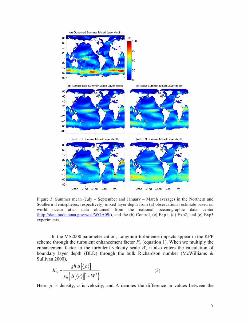
The 100-year mean (from model year 101 to 200) differences in the simulation verses Reynolds observed SST [obtained from the International Research Institute / Lamont-Doherty Earth Observatory Climate Data Library http://iridl.ldeo.columbia.edu/SOURCES/.IGOSS/.nmc/.Reyn_SmithOIv2/] are shown in Figure 2. Model summer and winter mean mixed layer depth (MLD) verses observational MLD [observational estimate are based on world ocean atlas data obtained from the national oceanographic data center (http://data.nodc.noaa.gov/woa/WOA09/)] are given in Figure 3 and 4. Both the observational and model MLD are calculated as the depth at which potential density (referenced to surface) changes by 0.125 kg m-3 from its surface values.

The main SST discrepancy between the model results and observations exists in the middle to high latitude regions, with a significant SST cold bias in the northern hemisphere and SST warm bias in the southern hemisphere. The cold biases are related to both an equatorward shift of the westerlies and extensive low cloudiness, and low values of shortwave radiation incident upon the surface (Delworth et al 2006). Neither of these biases are the focus of our study here. The SST warm biases found in the Southern Ocean are partially due to a positive shortwave radiation bias in the atmosphere model (Delworth et al 2006). We also suspect that the shallow summer MLD bias (Figure 3b) may in part be related to the lack of parameterized mixing associated with surface ocean gravity waves.

6

Figure 2. Maps of errors in simulation of annual-mean SST (°C) for the (a) Control, (b) Exp1, (c) Exp2, and (d) Exp3 experiments. The errors are computed as model minus observations, where the observations are from the Reynolds SST data [obtained from the International Research Institute / Lamont-Doherty Earth Observatory Climate Data Library http://iridl.ldeo.columbia.edu/SOURCES/.IGOSS/.nmc/.Reyn_SmithOIv2/]. The numbers under the panels give the SST root mean square error for the globe, the southern hemisphere (90S – 30S), the equatorial region (30S – 30N), and the northern hemisphere (30N – 90N).

a. Exp1: MS2000 Parameterization By implementing the MS2000 parameterization (Exp1), we anticipate deepening

the summer mixed layer depth and thus affecting the SST warm bias in the Southern ocean. Unfortunately, we see a larger SST bias globally in Exp1, with the SST root mean square error (RMSE) of 1.69 oC in Expt 1 verses 1.24 oC in the control experiment (Figure 2b). To better characterize the biases, we separate the globe into three zonal regions and calculate the RMSE for each region: Northern Hemisphere – 30oN to 90 oN; equator – 30oS to 30oN; and Southern Hemisphere – 30oS to 90 oS. The largest SST error increase in Exp1 is found in the northern hemisphere with 0.72 oC increase in RMSE, and the lowest increase is in the Southern Ocean with 0.06 oC increase in RMSE.

Strong deepening of the winter MLD was observed in Exp1 (Figure 4c). The MLD becomes especially deeper than observations in the mid-latitude storm track region. On the other hand, deepening of the summer MLD is negligible in both hemispheres (Figure 3c), thus leading to minimal impact on the warm SST bias in the Southern Ocean. These results suggest that too much turbulent mixing is introduced by the MS2000 parameterization during winter, yet not enough turbulent mixing in the summer.

7

Figure 3. Summer mean (July – September and January – March averages in the Northern and Southern Hemispheres, respectively) mixed layer depth from (a) observational estimate based on world ocean atlas data obtained from the national oceanographic data center (http://data.nodc.noaa.gov/woa/WOA09/), and the (b) Control, (c) Exp1, (d) Exp2, and (e) Exp3 experiments.

In the MS2000 parameterization, Langmuir turbulence impacts appear in the KPP

scheme through the turbulent enhancement factor Flt (equation 1). When we multiply the enhancement factor to the turbulent velocity scale W, it also enters the calculation of boundary layer depth (BLD) through the bulk Richardson number (McWilliams & Sullivan 2000),

Rib =gh ! !"# $%

!0 ! u"# $%2+W 2( )

(3)

Here, ρ is density, u is velocity, and Δ denotes the difference in values between the

8

surface and depth h, and the BLD is equal to the smallest value of h at which this Richardson number equals a critical value. Thus, a larger turbulent velocity scale (W) increases the BLD, whereas increases in stratification limit the deepening. Since the stratification is weak during the winter, enhancement of W will efficiently deepen the mixed layer. In the contrast, during the summer, the relatively strong stratification will restrain the deepening effect by the enhanced W.

Figure 4. Winter mean (January – March and July – September averages in the Northern and Southern Hemispheres, respectively) mixed layer depth from (a) observational estimate based on world ocean atlas data obtained from the national oceanographic data center (http://data.nodc.noaa.gov/woa/WOA09/), and the (b) Control, (c) Exp1, (d) Exp2, and (e) Exp3 experiments.

b. Exp2: Smyth et al (2002) Parameterization Smyth et al (2002) used the MS2000 scheme to study the upper ocean response to a westerly windburst in the equatorial Pacific. They found that the reduction in daytime warming is insufficient to reproduce the LES results quantitatively, while the application

9

of the MS2000 parameterization during nocturnal convection causes unrealistically rapid mixing throughout the mixed layer. Their finding is analogues to what we see in Exp1, where the MS2000 scheme generates too much mixing in the winter time and too little mixing in the summer. Smyth et al (2002) adjusted the MS2000 parameterization by adding the stratification effect. Instead of using Lw in equation (1) as a constant, they changed it to a function of friction velocity u* and the convective velocity scale w* (equation 2). Through their modification, the turbulent enhancement will be restrained under weak stratification conditions and magnified under strong stratification conditions.

By replacing the MS2000 parameterizations with the Smyth et al (2002) parameterization in Exp2, we find that the SST bias in CM2M is improved globally (Figure 2c) with a RMSE of 1.18 oC (verses 1.24 oC in the control). The major improvement is found in the Southern Ocean with a reduction of 0.21 oC in RMSE, while changes in the equatorial and northern hemisphere regions are small (± 0.05 oC). The reduction in Southern Ocean SST warm bias is associated with a deeper summer MLD simulated in Exp2 (Figure 3d) as compared to the control experiment (Figure 3b). Notice the Southern Ocean summer MLD in Exp2 is also deeper than Exp1, indicating the improvement for our model by using the Smyth et al (2002) parameterization verses MS2000.

The winter MLD in Exp2 (Figure 4d) is more reasonable compared with observations, including more mode and intermediate water formation in the Southern Ocean. Strong MLD deepening is observed in the Labrador Sea at comparable magnitude to the observations. And most interestingly, reduction of MLD is observed in the Weddell Sea and Ross Sea. CM2M produces unrealistically strong convection in these regions and thus generates very deep mixed layer of more than 2000 meters. The CCSM4 model also shows overly too deep MLD in the Weddell Sea (Figure 19, Danabasoglu et al 2012). Apparently, with the Langmuir turbulence parameterization, we are able to simulate more realistic MLD in these regions. We return to these features in later in this section.

Despite the improvement particularly in the Southern Ocean, the simulated summer MLD remains shallower than observations, and the SST remains too warm. We suggest here three possible reasons for the remaining bias. One reason could be due to the low resolution used in the atmosphere model, in which the strength of mid-latitude storms are underestimated – the highest wind speed resolved by our model is 26 m s-1, while the mid-latitude storms very often have wind speed exceeding 30 m s-1 (NCEP wind reanalysis http://nomad3.ncep.noaa.gov/ncp_data). A low bias in wind speed leads in turn to a low wind stress and smaller amplitude surface gravity waves. Thus, in the mid-latitude region, we have a low bias in both the wind stress and turbulent enhancement from Stokes drift, which results in lower turbulent mixing and a warmer SST. A related problem could be that more wave characteristics need to be taken into consideration in parameterizing the Langmuir turbulent effect, besides just the Langmuir number and stratification that we used. In particular, we suggest that the misalignment between the Stokes drift and wind (Van Roekel et al 2012), and the penetration depth of Stokes drift (Sullivan et al 2012) may be important for more accurately parameterizing Langmuir effects. Finally, the Southern Ocean SST warm bias may be dominated in our climate model by the positive shortwave radiation bias in the atmosphere model, particularly in the summer MLD and SST

10

c. Exp3: Qiao et al (2004) Parameterization Qiao et al (2004) used a different approach to parameterize the ocean surface

gravity wave induced turbulent mixing in the upper ocean. They proposed an adjustment to the vertical diffusivity and viscosity through integration of the wave spectrum. The physical idea is that the wave orbital velocity should enter the calculation of Reynolds stress. There is hence no clear separation between the Qiao et al (2004) approach and the MS2000 and Smyth et al (2002) approach, as the Stokes drift is the net residual of wave orbital motion. What makes Qiao et al (2004) a very different approach is that their parameterized adjustment solely depends on the wave characteristics and does not care where the boundary layer is located. This approach is compelling, as surface ocean gravity waves are not affected by ocean stratification.

Exp3 exhibits a reduction of 0.19 oC in RMSE relative to the control experiment in the Southern Ocean using the Qiao et al (2004) parameterization. However, the SST bias is increased elsewhere and globally (Figure 2d). The reduction in the SST warm bias in the Southern Ocean is mainly due to deepening of the summer MLD (Figure 3e) compared to the control (Figure 3b). Notice the Southern Ocean summer MLD in Exp3 is deeper than both Exp1 and Exp2. However, in the winter, there is minimal improvement in the MLD (Figure 4e). Instead, the MLD simulated in the Labrador Sea is even shallower than the control experiment. Even though the MLD in the Ross Sea is improved, the improvement in the Weddell Sea is very limited.

3.2 High Latitudes with the Smyth et al (2002) Scheme Over all, we consider the Smyth et al (2002) parameterization to give the most

compelling improvements for our climate simulations. Although these improvements are likely model dependent, it is instructive to more fully characterize some of the changes associated with the Exp2 using this scheme, with a focus on selected high latitude regions. As we will see, it is both the effects from increased vertical mixing arising from the parameterized Langmuir turbulence and lateral transport that leads to certain of the more intriguing, and sizable, impacts from this scheme.

a. Labrador Sea We start by considering the impacts in the Labrador Sea, where the control

experiment is found to underestimate the winter MLD. By adding extra turbulent mixing through the Langmuir turbulent parameterization in Exp2, the winter MLD was greatly deepened from the southern mouth of the Labrador Sea all the way to its northern end (Figure 4d). In doing so, the simulation produces a Labrador Sea MLD that is closer to observations. In particular, the maximum MLD increased from less than 500 meters to more than 2000 meters at some locations.

Labrador Sea is one of a few major open ocean deep convection sites in the world’s ocean (Marshall and Schott 1999). The precondition in the northern hemisphere autumn (October to December) is a very important factor for deep convection in the winter (January to March). The mean Langmuir turbulent enhancement factor, Flt (equations 1 and 2), ranges from 1.4 at the northern end of the Labrador Sea to about 2 at the mouth in the autumn (Figure 5a). The sea ice extents are quite similar between the control experiment and Exp2, and more northward compared with the observations. To gain more understanding of the differences between the Control and Exp2, we examine

11

the ocean state along a transect of the Labrador Sea indicated by the white line in Figure 5a.

Figure 5. Labrador Sea seasonal mean Langmuir turbulence enhancement factor Flt (determined by equation 1 and 2) in Exp2 for boreal (a) autumn and (d) winter. The thin black line, thick black line and gray line indicate ice extent (ice concentration greater than 15%) for the control experiment, Exp2, and observations respectively. Autumn mean vertical eddy diffusivity for (b) the control experiment and (c) Exp2 along the transect defined by the white line in (a). Winter mean vertical eddy diffusivity for (e) the control experiment and (f) Exp2 along the transect defined by the white line in (d). In (b), (c), (e) and (f), the white/black line represent boundary /mixed layer depth, and the gray bar on the top indicate model ice extent.

The vertical eddy diffusivity (Kλ) in the control experiment is relatively small along the transect (Figure 5b) during autumn, with shallow turbulent boundary layer depth (BLD) and MLD (~50 to 60 meters). This weak turbulent mixing cannot break the

12

strong stratification created in the summer due to surface warming. As a result, a thick cold layer lies between the warmer mixed layer and the thermocline (Figure 6a). The strong temperature barrier creates a strong stratification in the surface water column (Figure 6b), and makes it very hard for deep convection to occur in the winter.

Figure 6. Autumn mean (a) potential temperature, (b) potential density, and (c) winter mean potential density for the control experiment in the Labrador Sea. Autumn mean (d) potential temperature, (e) potential density, and (f) winter mean potential density for Exp2. In (c) and (f), the gray bar on the top indicate model ice extent.

In Exp2, due to the strong turbulent mixing caused by the Smyth et al (2002) Langmuir parameterization, the vertical eddy diffusivity (Kλ) is much stronger (Figure 5c) than the Control, resulting in a doubling of the BLD and MLD. The strong turbulent mixing efficiently mixes warmer thermocline water into the surface layer from the

(a) Control Potential Temperature, OND

50 52 54 56 58 60 62500

400

300

200

100

0(d) Exp2 Potential Temperature, OND

50 52 54 56 58 60 62

(oC)

0

1

2

3

4

5

6

(b) Control 0, OND

27.75

27.7

27.6

27.5

50 52 54 56 58 60 62500

400

300

200

100

0(e) Exp2 0, OND

27.75

27.7 27.6

27.5

50 52 54 56 58 60 6227

27.2

27.4

27.6

27.8

28

Latitude

(c) Control 0, JFM

27.7527.7

27.6

50 52 54 56 58 60 621500

1200

900

600

300

0

Latitude

(f) Exp2 0, JFM

27.75

27.6

50 52 54 56 58 60 6227

27.2

27.4

27.6

27.8

28

13

thermocline below. The enhanced vertical mixing reduces stratification and increases the horizontal density gradient, which leads to enhanced lateral transport that mixes the surrounding North Atlantic Water into the Labrador Sea. In particular, to the southeast of the Labrador Sea, the northwestern loop of the North Atlantic Current transports warm water past the exit of the Labrador Sea. These warm waters are transported into the Labrador Sea by the enhanced lateral transport from the mesoscale eddy parameterization. As a result, we see a warmer surface layer, and the strong cold barrier is gone (Figure 6d). Much weaker stratification is created at the surface and the weakly stratified warm interior water is brought closer to the surface (Figure 6e). This is a favorable precondition for deep convection to occur.

During the northern hemisphere winter (JFM), Flt is about the same magnitude as in the autumn. We see up to two times enhancement in the Labrador Sea in the ice free regions (Figure 5d). The ice extent in Exp2 (thick black line in Figure 5d) is closer to observations, while the ice extends more southeast in the control experiment and covers almost the entire Labrador Sea (thin black line in Figure 5d). The sea ice is transported into the Labrador Sea either by the Labrador currents, or through the Denmark Strait by the East Greenland Current. Since the surface temperature at the mouth of the Labrador Sea is much warmer in Exp2 (Figure 6d), the sea ice transported towards the Labrador Sea by the East Greenland Current melts before entering the Labrador Sea.

Since the ice extends all the way to the mouth of the Labrador Sea in the control experiment, there is no interaction between the strong winter storms and the Labrador Sea water, and thus, no momentum flux into the ocean in the ice covered region. Due to the strong surface stratification formed in the autumn, buoyancy loss due to ice formation in this region is not strong enough to erode the stratification and trigger deep convection. Therefore, the mixing activity beneath the ice is very low (i.e. the magnitude of Kλ is very small) (Figure 5e). Mixing at the mouth of the Labrador Sea is stronger compared to autumn due to strong winter storms. We can see weak deep convection penetrates to ~2000m depth. However, the deep convection is not strong enough to overcome the strong stratification built up in the autumn (Figure 6c). As a result, the mixed layer depth deepening is limited to only 200 to 300 meters, which is shallower than observations.

In Exp2, the ice extent is pushed into the northern end of the Labrador Sea, and the enhanced mixing create a weaker surface stratification in the autumn. When winter sets in, vigorous buoyancy loss due to surface cooling further erodes the near surface stratification, thus exposing the weakly stratified water mass beneath. Unlike the control case, this region is ice free, thus exposing the ocean to strong winter storms. The enhanced mixing further reduces stratification. Then the subsequent cooling events initiate deep convection, in which a substantial part of the fluid column overturns and distributes the dense surface water in the vertical. We can see very large eddy diffusivity from the surface all the way to almost 3000 meters depth (Figure 5f). The largest eddy diffusivity is found between 500 and 1000 m, and is ten times larger than the control experiment. As a result of the deep convection, the deep layer outcrops at the surface with very weak stratification beneath it (Figure 6f). The BLD has deepened to ~1300m, and the MLD has deepened to > 2500m. In contrast, for the control case, the stratification is largely maintained throughout winter.

The enhanced deep convection in the Labrador Sea in Exp 2 leads to ~1.5 Sv of increase in Atlantic Meridional Overturning Circulation (AMOC) compared with the

14

control experiment (not shown). AMOC carries warm upper waters into northern latitudes and returns cold deep waters across the Equator. Its large heat transport has a substantial influence on climate. Deep convection and bottom water formation in the Labrador Sea is an important factor influencing the strength of the AMOC (Delworth et al 2008). In Exp2, the heat transport is increased by around 10-20% in the middle to high latitudes of the Atlantic compared with the control experiment (not shown).

Figure 7. Southern Ocean seasonal mean Langmuir turbulence enhancement factor Flt (determined by equation 1 and 2) in Exp2 for (a) autumn and (d) winter. The thin black line, thick black line and gray line indicate ice extent (ice concentration greater than 15%) for the control experiment, Exp2, and observations respectively. Autumn mean vertical eddy diffusivity for (b) the control experiment and (c) Exp2 along the transect defined by the white line in (a). Winter mean vertical eddy diffusivity for (e) the control experiment and (f) Exp2 along the transect defined by the white line in (d). In (b), (c), (e) and (f), the white/black line represent boundary /mixed layer depth, and the gray bar on the top indicates model ice extent.

(a) Flt in AMJ

200 150 100 50 080

70

60

50

40(d) Flt in JAS

200 150 100 50 080

70

60

50

40

1

1.2

1.4

1.6

1.8

2

2.2

(b) Control K along transect in AMJ

70 65 60 55 50 45200

100

0

70 65 60 55 50 455000

4000

3000

2000

1000

(c) Exp2 K along transect in AMJ

70 65 60 55 50 45200

100

0

70 65 60 55 50 455000

4000

3000

2000

1000

(e) Control K along transect in JAS

70 65 60 55 50 45200

100

0(m2 / s)

0

0.05

0.1

0.15

0.2

0.25

70 65 60 55 50 455000

4000

3000

2000

1000

(f) Exp2 K along transect in JAS

70 65 60 55 50 45200

100

0(m2 / s)

0

0.05

0.1

0.15

0.2

0.25

70 65 60 55 50 455000

4000

3000

2000

1000

15

b. Weddell Sea The Control experiment produces unrealistically strong convection in the Ross

Sea and Weddell Sea regions, and generates a very deep mixed layer of more than 2000 meters in the winter (Figure 4b). CCSM4 also shows the same very deep mixed layer in the Weddell Sea (Figure 19, Danabasoglu et al 2012). After applying the Smyth et al (2002) Langmuir turbulence parameterization in Exp2, the MLD is reduced in both seas for our simulations (Figure 4d).

Figure 8. Weddell Sea initial condition of (a) salinity, and (b) potential density along the transect defined in Figure 5. Winter mean (c) salinity, and (d) potential density for the control experiment. Winter mean (e) salinity, and (f) potential density for Exp2. In (c) to (f), the white/black line represent boundary /mixed layer depth, and the gray bar on the top indicates model ice extent.

The mean Langmuir turbulent enhancement factor, Flt, shows similar magnitude in the Weddell and Ross Seas as found in the Labrador Sea, for both the austral autumn

16

(AMJ) and winter (JAS) (Figure 7 a, d). The Southern Ocean sea ice extent in the Control and Exp2 are very close to each other in the autumn, and virtually the same in the austral winter. The model sea ice growth is slower than observations for both seasons. To understand the mechanism for MLD reduction in the Ross Sea and Weddell Sea, we examine certain of the ocean responses along a transect in the Weddell Sea indicated by the white line in Figure 7 a and d.

In the Weddell Sea, the water column is well stratified with depth (Figure 8b). The water to the south of 55oS is under sea ice during most of the year and thus much colder and saltier than the water north of it. The salinity and temperature contrast are especially large in the top 100 meters. Furthermore, the water is up to 1 psu saltier (Figure 8a) and more than 6oC colder than the water north of 55oS (not shown). Deep convection is triggered by the thermobaric effect, which arises from the pressure dependence of the thermal expansion coefficient, with Gill (1973) and Killworth (1979) first recognizing the role of the thermobaric effect in their calculations/models of hydrostatic stability in the Weddell Sea.

Along the Weddell Sea transect, the distribution of vertical eddy diffusivity (Kλ) does not change much with season (Figure 7). Deep mixing occurs beneath the mixed layer year round for both the control experiment and Exp2. Ideal age (the age since water was last at the surface) is one way of looking at differences in ventilation. Figure 9 presents the ideal age of the two simulations averaged between model year 181 to 200. The Control experiment shows strong deep ventilation occurring to the south of 55 oS, and penetrating all the way to more than 4000 meters deep, while Exp2 only shows weak ventilation in the top 1000 meters or so. One possible reason for enhanced ventilation in the control experiment could be that there is not enough lateral tansport to draw stratified water into the ventilated region from the periphery and stabilize it after winter has passed.

The strong year round deep ventilation in the Control experiment creates a well mixed deep layer beneath the boundary layer (Figure 8c, d), which hardly varies with seasons (not shown). Deep ventilation is much weaker in Exp2 and unable to fully mix the deep layer like the Control experiment, yet it reduces stratification in the water column (Figure 8f) compared to the initial condition (Figure 8b). Stratification of the water column beneath the boundary layer also hardly changes with season (not shown). Thus, it is the seasonal variation in the boundary layer that determines the MLD in both experiments.

As sea ice melts in the summer, the surface water becomes fresher and is warmed to about 4oC. The BLD and MLD become their shallowest during the year (~ 50 m), but the water beneath remains cold and thus creates a thermal barrier between the top layer and the ocean interior (not shown). In Exp2, the enhanced Langmuir turbulent mixing efficiently mixes more cold water into the boundary layer from below, which also increases the north-south lateral density gradient in the upper ocean. The increased density gradient leads to enhanced baroclinicity and an associated increased lateral transport through parameterized mesoscale eddies that mixes fresher water from the periphery north of the ice boundary into the boundary layer. These processes create a deeper, colder and fresher boundary / mixed layer compared with the Control experiment (not shown).

17

Figure 9. Autumn 20 year mean (model year 181 – 200) age for (a) the control experiment and (b) Exp2 along the Weddell Sea transect defined in Figure 6a. Winter 20 year mean age for (c) the control experiment and (d) Exp2 along the Weddell Sea transect. The gray bar on the top indicate model ice extent.

Sea ice starts to grow back in the autumn. The enhanced Langmuir turbulent mixing (Figure 7c) together with enhanced lateral transport continues to mix more cold water from beneath and fresh water from the periphery into the boundary layer, and keeps the boundary layer deeper, colder and fresher compared to the Control experiment (not shown). When winter sets in, vigorous ice formation reduces the surface stratification by making the surface water colder and saltier. In Exp2, intense winter storms together with large surface waves create strong turbulent mixing in the water column (Figure 7f), which is about three times the turbulent mixing than the Control experiment (Figure 7e). This strong turbulent mixing together with enhanced lateral transport efficiently mixes fresher water into the boundary layer from the periphery and keeps the surface stratification strong (Figure 8e and f). Due to the strong saline stratification build up on the surface, deep convection is greatly inhibited in Exp2, and is thus much weaker than the Control experiment (Figure 7e, 7f). Owing to the strong surface stratification and week convection, stratification is maintained beneath the mixed layer in Exp2 (Figure 8f).

For the Control experiment, the turbulent mixing and lateral transport are weaker compared to Exp2 in all seasons. As a result, the surface water is saltier and warmer in the summer. When sea ice starts to grow back in the autumn, the surface water becomes saltier due to ice formation. The weak turbulent mixing and lateral transport cannot mix enough fresher water from the periphery and the saline stratification becomes even

(a) Control Age in AMJ

70 65 60 55 50 455000

4000

3000

2000

1000

0(b) Exp2 Age in AMJ

70 65 60 55 50 455000

4000

3000

2000

1000

0

(c) Control Age in JAS

70 65 60 55 50 455000

4000

3000

2000

1000

0(d) Exp2 Age in JAS

70 65 60 55 50 455000

4000

3000

2000

1000

0

Age (year)

10 40 70 100 130 160 190

18

weaker. When winter sets in, vigorous ice formation further reduces the surface saline stratification and triggers strong deep convection, while the weak turbulent mixing and lateral transport cannot mix enough fresher water from the periphery, in contrast to Exp2. Thus, the surface stratification is further reduced and matches with the interior water to produce a very deep mixed layer as diagnosed by the MLD criteria (potential density changes by 0.125 kg m-3 from its surface values). As a result, even though the BLD is deeper in Exp2, the MLD depth is much deeper in the Control experiment. 4. Summary and Discussions In this study, the effect on simulated global climate from parameterized mixing associated with surface ocean gravity waves is assessed through modification to the K-profile ocean boundary layer parameterization (Large et al 1994). Our tool for this assessment is a fully coupled atmosphere-ocean-wave global climate model. In this coupled system, WAVEWATCH III, the operational wave model developed and used at NCEP, is incorporated into the GFDL climate model CM2M. Two Langmuir turbulence parameterizations and one non-breaking wave parameterization are evaluated using the fully coupled system.

For our simulations, the McWilliams & Sullivan (2000) Langmuir parameterization produced too much turbulent mixing during winter, yet not enough turbulent mixing in the summer. In their scheme the Langmuir turbulence effect is brought into KPP through an enhancement factor (Flt) that multiplies the turbulent velocity scale W. Thus, Flt also enters the calculation of boundary layer depth (BLD) through the bulk Richardson number. A larger W, as from Langmuir turbulence, works to increase the BLD, while stratification works to limit the deepening. Since the stratification is weak during winter, enhancement of W deepens the mixed layer. In contrast, during summer the stronger stratification will restrain the deepening effect from their scheme.

The Smyth et al (2002) parameterization includes stratification impacts to the McWilliams & Sullivan (2000) parameterization so that the turbulent enhancement is restrained under weak stratification conditions and magnified under strong stratification conditions. By using the Smyth et al (2002) parameterization, our simulated SST bias is improved globally compared with the original CM2M results (the root mean square error is improve by 6%). The largest improvement is found in the Southern Ocean and is associated with a deeper summer MLD (the root mean square error is improved by 15%), although the model simulated summer MLD is still shallower than observations.

Although the Smyth et al (2002) scheme reduced the Southern Ocean biases in SST and MLD, we suggest that other biases or limitations may need to be addressed in our simulations to further reduce the biases. One important reason could be that due to the low resolution used in the atmosphere model, the intensity of mid-latitude storms is underestimated, which in turn lead to smaller (height and length) surface ocean waves. Thus, in the mid-latitude region, we a have low bias in both the wind stress and turbulent enhancement due to Stokes drift, which in turn result in lower turbulent mixing and warmer SST. This result points to the intimate relation between parameterized surface ocean gravity wave mixing and the atmospheric model simulation. Relatedly, we could be encountering limitations of the Langmuir mixing parameterizations considered here, in

19

which more wave characteristics may need to be taken into consideration, besides the Langmuir number and stratification, such as the misalignment between the Stokes drift and wind (Van Roekel et al 2012), and the penetration depth of Stokes drift (Sullivan et al 2012). Another possibility for the remaining shallow MLD bias may be related to the positive shortwave radiation bias in the atmosphere model in the Southern Ocean (Delworth et al 2006). Qiao et al (2004) argue that the wave orbital velocity should enter the calculation of Reynolds stress. They proposed an adjustment to the vertical diffusivity / viscosity through integration of the wave spectrum. What makes Qiao et al (2004) a very different approach is that their parameterized adjustment solely depends on the wave characteristics and does not care about the boundary layer. Their parameterization provides the strongest summer MLD deepening in the Southern Ocean among the three experiments, but the effects are very weak elsewhere and during the winter. Since the Stokes drift is the net residual of wave orbital motion, there is no clear separation between the Qiao et al (2004) approach and the MS2000 and Smyth et al (2002) approach, so these schemes should not be applied together.

With the Smyth et al (2002) parameterization, strong MLD deepening is observed in the Labrador Sea bringing the simulated MLD to a comparable magnitude to the observations. And surprisingly, reduction of MLD is found in the Weddell Sea and Ross Sea, also bringing simulations into better agreements with observations. Through analyzing the model behavior at the Labrador Sea and the Weddell Sea separately, we found that even though the Langmuir turbulence parameterization is applied to enhance the vertical mixing in the KPP scheme, the coupling with enhanced lateral transport is the key for improving MLD simulations. Our results suggest that the enhanced vertical mixing creates lateral variations in the temperature and salinity fields, which lead to enhanced lateral transport. Through enhanced lateral transport, more warm water is brought into the Labrador Sea from the periphery. The warm water melts the ice and reduces surface stratification through enhanced vertical mixing, and creates an ideal condition for deep convection in the winter. In the Weddell Sea, enhanced lateral transport brings saltier water from the periphery and increases surface stratification through enhanced vertical mixing, which inhibits deep convection and reduces MLD. 5. Closing Remarks There are several processes that affect upper ocean mixing, such as mesoscale eddies, submesoscale eddies, convection, and Langmuir turbulence. The interactions among these processes are complex and may lead to unexpected behavior, such as that found in our simulations in which the mixed layer greatly shallowed in the Weddell Sea relative to the control simulation. We do not presume our model results are in any way the final word on these interactions. Yet we suggest they point to the importance of gauging the impact from ocean surface gravity wave mixing within the context of a realistic climate simulation. Given computational limitations, current large-scale climate models are incapable of explicitly resolving certain of the complex physical processes evolved in upper ocean mixing. Since upper ocean process are crucial in determining atmosphere-ocean fluxes in

20

climate models, the development of upper ocean mixing parameterization is an area that deserves extensive research efforts. In particular, the different behavior of the two Langmuir turbulence parameterization schemes used in this study suggest that more physical pieces may be needed in the parameterizations, besides Stokes drift. Further tuning of the coefficients in the Smyth et al (2002) parameterization did not give better results (not shown), which also emphasizes the need for better understanding of the physics of Langmuir turbulence.

Many wave dependent processes are currently parameterized within coupled ocean-atmosphere general circulation models using wind-dependent parameterizations (Cavaleri et al., 2012). This is a valid simplification if winds and waves are in equilibrium. However, Fan et al (2013) shows this is not the case over the majority of the ocean, with swell dominating the global wave field. To demonstrate this effect, we compared the wind speed parameterized surface Stokes drift with wave model generated Stokes drift in Appendix B. Our results suggest that the wind-dependent parameterized Stokes drift is not a good representation of the wave model generated Stokes drift, and this result emphasizes the need for a wave model in the coupled climate models. We close our paper by offering a speculation for one area where ocean surface gravity waves may play a significant role in climate change. Namely, as Arctic sea ice melts, the upper ocean is exposed to mixing by ocean surface waves that were previously absent. Such mixing may in turn erode the Arctic pycnocline which separates the upper Arctic Ocean from the warm Atlantic waters at intermediate depths. In particular, during the boreal Autumn, when the mid-latitude storms become strong and are accompanied by large ocean surface gravity waves, the sea ice area in the Arctic Ocean also reaches its minimum. Strong surface gravity wave induced turbulent ocean mixing can reduce the surface stratification and provide the necessary precondition for convection in the Arctic Ocean. In so doing, this enhanced ventilation could release heat from the deep Arctic, thus accelerating sea ice melt. We suggest that this role for surface ocean gravity waves may be critical for projecting Arctic climate change over the coming decades. Appendix A. Physical components of CM2M

The physical components of CM2M include four models: atmosphere, land, sea

ice, and ocean. The atmospheric model version 2 (AM2) uses a finite volume dynamic core, and

has a grid spacing of 2.5° longitude by 2° latitude and 24 vertical levels. The model contains a suite of model physics including cloud prediction and boundary layer schemes, and diurnally varying solar insolation. The radiation code allows for explicit treatment of numerous radiatively important trace gases (including tropospheric and stratospheric ozone, halocarbons, etc.), a variety of natural and anthropogenic aerosols (including black carbon, organic carbon, tropospheric sulfate aerosols, and volcanic aerosols), and dust particles. Aerosols in the model do not interact with the cloud scheme, so that indirect aerosol effects on climate are not considered.

The ocean component of CM2M employs the MOM4p1 code of Griffies (2009) configured with the same grid and bathymetry as the CM2.1 ocean component (Gnanadesikan et al. 2006; Griffies et al. 2005). The new features in MOM4p1 are given in details in Dunne et al (2012a). MOM4p1 uses a tripolar grid with 1° grid spacing in

21

latitude and longitude north/south of 30°N/30°S. The meridional resolution becomes progressively finer equatorward and reaches about 1/3° at the equator. The poles are set over Eurasia, North America, and Antarctica to avoid polar filtering over the Arctic. The model has 50 vertical levels, including 22 levels with10-m thickness each in the top 220 m.

The Land Model, version 3 (LM3) is utilized in CM2M. LM3 is a new model for land water, energy, and carbon balance. In comparison to its predecessor, Milly and Shmakin (2002), LM3 includes more comprehensive models of snowpack, soil water, frozen soil–water, groundwater discharge to streams, and finite-velocity horizontal transport of runoff via rivers to the ocean. LM3 uses the same grid configuration as the atmospheric model.

The sea ice model is a dynamical model with three vertical layers and five ice thickness categories. The model uses the elastic viscous plastic rheology to calculate ice internal stresses, and a modified Semtner three-layer scheme for thermodynamics (Winton 2000). Appendix B. Surface Stokes Drift Parameterization

Li and Garrett (1993) proposed a simple surface Stokes drift, Us(0)

parameterization as a function of the 10-m wind speed, Uw. Us(0) = 0.016 Uw (B1)

We randomly take a snapshot of 10-m wind speed from our coupled model during the boreal winter and parameterized Us(0) using equation (B1) as shown in Figure B1 (b). The corresponding surface Stokes drift calculated from our coupled model is given in Figure B1 (a), and the difference between them are given in Figure B1 (c). We can see that the parameterized Stokes drift is larger than the model generated Stokes drift almost everywhere in the global ocean, and the differences are stronger in the mid-latitude storm region.

To reduced the differences between the parameterized and model simulated Stokes drift, we adjusted the Parameter in (B1) from 0.016 to 0.0067 so that the root mean square error between the parameterized and model simulated surface Stokes drift are at the minimum. The percentage of the difference between the adjusted parameterized Stokes drift and the model simulated values relative to the model simulated values are given in Figure B1 (d). We can see both overestimates and underestimates of in the mid-latitude region and overestimates in the tropical region. The overestimations are more than 100% in a large area of the global ocean, and the underestimations are up to 100% at many places as well. We also tried to adjust the parameterized surface Stokes drift based on matching its mean value, maximum value or standard deviation with the model simulated surface Stokes drift, but none of our attempts reduces the differences. Thus, we conclude that the wind-dependent parameterized Stokes drift is not a good representation of the wave model generated Stokes drift.

22

Figure B1. Surface stokes drift from the (a) wave model and (b) Li & Garrett Parameterization, (c) their differences (b minus a), and (d) the percentage of differences between the adjusted surface stokes drift from Li & Garrett Parameterization and the wave model simulated surface stokes drift relative to the model simulated surface stokes drift. Note, (a) and (b) share the same color bar. References: Babanin, A. V, A. Ganopolski, and W. R.C. Phillips, 2009: Wave-induced upper-ocean

moxing in a climate model of intermediate complexity. Ocean Modeling, 29, 189-197.

Bates, S. C., B. Fox-Kemper, S. R. Jayne, W. G. Large, S. Stevenson, and S. G. Yeager, 2012: Mean Biases, variability, and trends in air-sea fluxes and Sea Surface Temperature in the CCSM4. J. Clim., 25(22), 7781-7801

Beljaars, A. C. M., 1994: The parameterization of surface fluxes in large-scale models under free convection. Q. J. R. Meteorol. Soc. 121, 255-270.

Chen, G., B. Chapron, R. Ezraty, and D. Vandmark, 2002: A global view of swell and wind sea climate in the ocean by satellite altimeter and scatterometer. J. Atmos. Oceanic Technol., 19, 1849-1859.

Craik, A. D. D. & Leibovich, S. 1976 A rational model for Langmuir circulations. J. Fluid Mech. 73, 401–426.

Danabasoglu, G, and Coauthors, 2012: The CCSM4 ocean component. J. Clim., 25, 1361 – 1389. DOI: 10.1175/JCLI-D-11-00091.1

Delworth, T., and Coauthors, 2006: GFDL’s CM2 global coupled climate models. Part I: Formulation and simulation characteristics. J. Climate, 19, 643–674.

23

Delworth, T., and coauthors, 2008: The potential for abrupt change in the Atlantic Meridional Overturning Circulation, Abrupt Climate Change: Final Report, Synthesis & Assessment Product 3.4, CSSP, Reston, VA, U.S. Geological Survey, 258-359.

Dunne, J. P., and co-authors, 2012 a: GFDL’s ESM2 global coupled climate-carbon earth system models Part I: physical formulation and baselines simulation characteristics. J. Clim. 25(19), doi: 10.1175/JCLI-D-11-00560.1

Dunne, J. P, and co-authors, 2012 b: GFDL’s ESM2 global coupled climate-carbon Earth System Models Part II: Carbon system formulation and baseline simulation characteristics. J. Clim. 26(7), doi: 10.1175/JCLI-D-12-00150.1

Fan, Y., S. Lin, I. M. Held, Z. Yu, and H. L. Tolman, 2012: Global Ocean Surface Wave Simulation using a Coupled Atmosphere-Wave Model. J. Clim. Vol. 25, 6233-6252

Fan, Y., I. M. Held, S. Lin, and X. Wang, 2013: Global Ocean Wave Climate Change Scenarios for the end of the 21st Century. J. Clim. In press

Fan, Y., S. Lin, S. M. Griffies, and M. A. Hemer, 2013: Simulated Global Swell and Wind Sea Climate and Their responses to Anthropogenic Climate Change at the End of the 21st Century. J. Climate, under review

Gill, A., 1973: Circulation and bottom water in the Weddell Sea, Deep Sea Res., 20, 111–140

Gnanadesikan, A., and Coauthors, 2006: GFDL’s CM2 global coupled climate models. Part II: The baseline ocean simulation. J. Climate, 19, 675–697.

Griffies, S. M., and Coauthors, 2005: Formulation of an ocean model for global climate simulations. Ocean Sci., 1, 45–79.

Griffies, S. M., 2009: Elements of MOM4p1. GFDL Ocean Group Tech. Rep. 6, 377. [Website: http://data1.gfdl.noaa.gov/~arl/pubrel/o/old/doc/mom4p1_guide.pdf ]

Gong, D. and Wang, S., 1999: Definition of Antarctic oscillation index, Geophys. Res. Lett., 26, 459–462, doi:10.1029/1999GL900003.

Hanley K. E., S. E. Belcher, and P. P. Sullivan, 2010: A Global Climatology of Wind-Wave interaction. J. Phys. Oceanogr. 1263-1282.

Hasselmann, K., 1970: Wave-driven inertial oscillations. Geophys. Fluid Dyn., 1, 463–502.

Ho, M, A. S. Kiem, and D. C. Verdon-kidd, 2012: The southern annular mode: a comparison of indices. Hydrol. Earth Syst. Sci., 16, 967–982.

Huang, N. E. 1979: On surface drift currents in the ocean. J. Fluid Mech. 91, 191-208. Jullion, L., S. C. Jones, A. C. Naveira Garabato, and M. P. Meredith, 2010: Wind-

controlled export of Antarctic Bottom Water from the Weddell Sea. Geophys. Res. Lett. 37, L09609, doi:10.1029/2010GL042822.

Killworth, P. D., 1979: On chimney formation in the ocean, J. Phys. Oceanogr., 9, 531–554.

Large, W. G., J. C. McWilliams, and S. C. Doney, 1994: Ocean vertical mixing: a review and model with a nonlocal boundary layer parameterization. Reviews of Geophysics, 32, 4, 363-403

Lavender, K. L., R. E. Davis, and W. B. Owens, 2000: Mid-depth recirculation observed in the interior Labrador and Irminger Seas by direct velocity measurements. Nature, 407, 66–69.

24

Leibovich, S., 1977a: On the evolution of the system of wind drift currents and Langmuir circulations in the ocean. Part 1. Theory and averaged current. J. Fluid Mech., 79, 715–743.

——, 1977b: Convective instability of stably stratified water in the ocean. J. Fluid Mech., 82, 561–585.

Li, M., K. Zahaiev, and C. Garrett, 1995: Role of Langmuir circulation in the deepening of the ocean surface mixed-layer, Science, 270, 1955– 1957.

Meredith, M. P., P. L. Woodworth, C. W. Hughes, and V. Stepanov (2004), Changes in the ocean transport through Drake Passage during the 1980s and 1990s, forced by changes in the Southern Annular Mode, Geophys. Res. Lett., 31, L21305, doi:10.1029/2004GL021169.

Milly, P. C. D., and A. B. Shmakin, 2002: Global modeling of land water and energy balances. Part I: The land dynamics (LaD) model. J. Hydrometeor., 3, 283–299.

McWilliams JC, Sullivan PP. 2000. Vertical mixing by Langmuir circulations. Spill Sci. Technol. Bull. 6:225–37

_____, P. P. Sullivan, and C.-H. Moeng, 1997: Langmuir turbulence in the ocean. J. Fluid Mech. 334, 1–30.

Najjar, R. G., and co-authors, 2007: Impact of circulation on export production, dissolved organic matter and dissolved oxygen in the ocean: results from Phase II of the Ocean Carbon‐cycle Model Intercomparison Project (OCMIP‐2). Global Biogeochem. Cycles, 21, p. GB3007.

Pickart, R. S., 1997: Adventure in the Labrador Sea: A wintertime cruise to the North Atlantic. Oceanus, 40 (1), 18–24.

Qiao, F., Y. Yuan, Y. Yang, Q. Zheng, C. Xia, and J. Ma, 2004: Wave-induced mixing in the upper ocean: Distribution and application to a global ocean circulation model. Res. Lett. 31, L11303, doi:10.1029/2004GL019824, 2004

Sarmiento, J. L., N. Gruber, M. Brzezinski, and J. P. Dunne, 2004: High-latitude controls of thermocline nutrients and low latitude biological productivity. Nature, 427, 56-60.

Skyllingstad E. D., W. D. Smyth, and G. B. Crawford, 2000: Resonant wind-driven mixing in the ocean boundary layer. J. Phys. Oceanogr., 30, 1866-1890.

Smyth, W. D., E. D. Skyllingstad, G. B. Grawford, and H. Wijesekera, 2002: Nonlocal fluxes and Stokes drift effects in the K-profile parameterization. Ocean Dyn. 52, 104-115, DOI 10.1007/s10236-002-0012-9

Sullivan P. P., J. C. McWilliam, and W K. Melville, 2007: Surface gravity wave effects in the oceanic boundary layer: large-eddy simulation with vortext force and stochastic breakers. J. Fluid Mech., 593, 405-452.

Sullivan P. P. and J. C. McWilliam, 2010: Dynamics of Winds and Currents Coupled to Surface Waves. Annu. Rev. Fluid Mech. 2010. 42, 19-42.

Sullivan, P. P., Romero, L., McWilliams, J. C., Melville, W. K., 2012. Transient evolution of Langmuir turbulence in ocean boundary layers driven by hurricane winds and waves. J. of Phys. Oceanogr. 42, 1959–1980.

Sy, A., M. Rhein, J. R. N. Lazier, K. P. Koltermann, J. Meincke, A. Putzka, and M. Bersch, 1997: Surprisingly rapid spreading of newly formed intermediate waters across the North Atlantic Ocean. Nature, 386, 675–679.

25

Thompson, D. W. J. and Wallace, J. M., 2000: Annular Modes in the Extratropical Circulation, Part I: Month-to-Month Variability, J. Climate, 13, 1000–1016.

Tolman, H. L., 1998: Validation of a new global wave forecast system at NCEP. Ocean Wave Measurements and Analysis, B. L. Edge and J. M. Helmsley, Eds., ASCE, 777-786.

Van Roekel, L. P., Fox-Kemper, B., Sullivan, P. P., Hamlington, P. E., Haney, S. R., 2012. The form and orientation of Langmuir cells for misaligned winds and waves. Journal of Geophysical Research – Oceans, 117, C05001, 22pp.

Winton, M., 2000: A reformulated three-layer sea ice model. J. Atmos. Oceanic Technol., 17, 525–531.

Weijer, W. B. M. Sloyan, M. E. Maltrud, N. Jeffery, M. W. Hecht, C. A. Hartin, E. V. Sebille, I. Wainer, and L. Landrum, 2012: The Southern Ocean and its climate in CCSM4, J. Clim. 25, 2652-2675, DOI: 10.1175/JCLI-D-11-00302.1