1

Occurrence probability of moderate to large earthquakes

in Italy based on new geophysical methods

Dario Slejko(1), Alessandro Caporali(2), Mark Stirling(3)

& Salvatore Barba(4)

(1) Nat. Inst. Oceanography and Experimental Geophysics, Trieste, Italy (2) University of Padova, Italy (3) GNS Science, Lower Hutt, New Zealand (4) Istituto Nazionale di Geofisica e Vulcanologia, Rome, Italy

Abstract We develop new approaches to calculating 30-year probabilities for

occurrence of moderate-to-large earthquakes in Italy. Geodetic techniques and finite-element modelling, aimed to reproduce a large amount of neotectonic data using thin-shell finite element, are used to separately calculate the expected seismicity rates inside seismogenic areas (polygons containing mapped faults and/or suspected or modelled faults). 30-year earthquake probabilities obtained from the two approaches show similarities in most of Italy: the largest probabilities are found in the southern Apennines, where they reach values between 10% and 20% for earthquakes of MW≥6.0, and lower than 10% for events with an MW≥6.5. Key words: seismic hazard; strong earthquakes; probability; Italy

1. Introduction Plate tectonics processes produce deformation within the crust of the

Earth, and the measurement of such surface deformation is an important boundary condition constraint on the interaction of crustal blocks through time. The distribution in space and time of geodetically derived strain rate will correlate, to some degree, with the geometry and activity of the underlying seismogenic sources, as well as with aseismic processes. In this context, many studies around the world have used geodetic strain rates to estimate earthquake recurrence and probability, providing a valuable supplement or alternative to parameters derived from geologic and seismic catalogue data.

During the period spring 2005 to summer 2007 the Department of the Italian Civil Protection funded several seismological and volcanological projects. One of the seismological projects was entitled “Assessing the seismogenic potential and the probability of strong earthquakes in Italy” (designated S2) and its main goals were: 1) to identify of the seismic sources capable of generating destructive earthquakes (i.e. events with a magnitude larger than 5.5), and 2) to assess the occurrence probability of

2

these events for the sources. The S2 project was organized in 4 tasks, and Task 4 was dedicated to the actual computation of the occurrence probabilities. One of the goals was to assess the occurrence probability of strong earthquakes using seismological information, and to calibrate the results with geodetic data. Our working hypothesis is that large earthquakes occur along major faults according to the characteristic earthquake model (Schwartz and Coppersmith, 1984). According to this hypothesis, faults show a tendency to generate earthquakes of similar characteristics (magnitude, slip, rupture length, etc.). While considered overly simplistic by the Italian research community, the characteristic earthquake model is useful as a basis for the broad data-based and methodological comparisons made in this study.

Our efforts are strongly motivated by the need to find ways to augment the incomplete coverage of fault mapping in Italy to date. While the fault dataset is considered to be 95% complete in the southern Apennines, it is at best only 70% complete in the rest of the country, and 50% complete or less in the offshore (Valensise, personal communication).

Considerable international literature is available regarding the evaluation of the occurrence probability of strong earthquakes on well defined faults (e.g. WGCEP, 2003) and the assessment of time independent (e.g.: Frankel et al., 2000) and time dependent seismic hazard (California: B1 2007 WGCEP, 2008; Italy: Peruzza, 2006). However, two main problems thwart these efforts in Italy: 1) the knowledge of the seismogenic faults in Italy is incomplete in terms of the number of faults and their geometric and seismic characteristics, and 2) constraints from geodetic data are problematic because the number of permanent GPS stations in Italy is small, the fact that they have only been in operation a short time interval (about 5 years), and the campaign measurements provide velocities with a large associated uncertainty. Not surprisingly, areal seismogenic sources were defined for areas suspected to contain fault sources as yet unmapped in the Database of the Italian Seismogenic Sources, see Basili et al. (2008) for details]. The specific application of these seismogenic area definitions was intended in the S2 project for estimation of earthquake recurrence parameter estimates for the Italian Seismogenic Source Database from geodetically-measured strain rate. Specifically, the geodetic strain rate would be converted into seismic moment rate (M0R) and then used to give an upper limit to the seismic potential of the seismogenic sources. Critical to this approach would be the assessment of M0R from GPS data, the association of this M0R to a geographical area, and the exact definition of a seismogenic source within the geographical area.

Our paper summarizes work undertaken thus far in the framework of the S2 project for the assessment of the occurrence probability in 30 years of moderate-to-large earthquakes within seismogenic areas defined in the Italian Seismogenic Source Database. We develop estimates of M0R from: 1) observations from permanent GPS stations (geodetic constraint), and 2) from a 3D geophysical model that incorporates state-of-the-art

3

knowledge on faults, and rheology, and is calibrated from GPS observations (geophysical constraint: Barba, 2007).

2. Basic ideas Two types of seismogenic sources are defined in the Italian

Seismogenic Source Database (Fig. 1). These are mapped faults and seismogenic areas. The mapped faults are generally well constrained from geological and geophysical data, in that a complete geometric and seismic parameterisation (length, dip, slip rate, slip-per-event etc.) are available, along with an evaluation of the uncertainties associated with the source parameters.

Seismogenic areas do not contain mapped faults, but are assumed to produce earthquakes of magnitude 5.5 or greater based on other geological, geomorphological and geophysical data. Features such as linear valleys along strike from the mapped faults are assumed to be fault controlled, but the lack of field mapping prevents the definition of fault sources at the present time. For the seismogenic areas, the polygon defining the overall source is given in the Italian Seismogenic Source Database, along with the associated parameters (depth, strike, dip, rake, and slip rate, expected maximum magnitude) and uncertainty bounds.

The research documented here is aimed at defining the seismic potential of the seismogenic areas from the present strain rate in Italy and in consideration of regional seismicity patterns. As not all the existing faults in the seismogenic areas are known, a statistical procedure was designed (Stirling et al., 2007) to fill the empty space of the seismogenic areas with modelled faults of rupture lengths similar to those of the known fault sources.

The working hypotheses of the present study are as follows: a) the regional geodetic strain is proportional to the seismic potential of

the region (i.e. strain is released by earthquakes and aseismic creep);

b) the earthquakes occur on a pre-defined set of faults (a combination of mapped faults and modelled faults: the total number of faults in each seismogenic area is given by the sum of the mapped and modelled faults);

c) faults produce earthquakes according to the characteristic earthquake model (i.e. a tendency to produce a narrow range of earthquakes at or near the maximum size possible from physical constraints such as fault length) and the total regional moment rate (M0R) is released as the sum of characteristic earthquakes;

d) the general magnitude-frequency distribution of a region is described by the Gutenberg– Richter behaviour, i.e. at the regional scale, the frequencies of the characteristic earthquakes form a Gutenberg– Richter distribution whose b-value is in agreement with the regional b-value, obtained by the past seismicity. According to the above hypotheses we assume that in the long term

4

(104-106 years), the majority of regional seismic release (proportional to

the regional geodetic strain) will occur on the mapped or modelled faults, each acting according to the characteristic earthquake model and all together representing a Gutenberg– Richter behaviour.

3. The data The network of some 160 permanent GPS stations has been in

operation for a decade (1995-2005) and as part of the European Permanent Network of EUREF and the CERGOP 2 Project of the European Union. Additional local densification stations provide a valuable contribution to the estimate of the average surface strain rate. The strain rate budget for central Europe, determined from GPS observations, is of the order of 20–40 nanostrain per year in a circular area of 150-200-km radius of the eastern Alps (see Fig. 2 where a 100-km ray is shown), corresponding to a velocity range of a few mm/year over distances of some hundreds of km (Caporali et al., 2008).

We compute velocity gradients by least squares co-location, which is a minimum variance algorithm capable of rigorously taking into account the stochastic properties of the input velocities (Caporali et al., 2003). For this purpose a covariance function is needed in order to represent the fall off of the correlation coefficient with the lag distance (average distance between the stations). Once the covariance function has been assigned then the velocity and the associated uncertainties can be computed at any point. For deformation analyses it is crucial to know how velocity changes spatially. The horizontal velocity gradient can be split into a symmetric and an anti-symmetric part. The symmetric part represents strain rate, whereas the anti-symmetric part represents a rigid rotation and is, hence, ignorable for deformation studies as the rigid rotation has no associated deformation. The symmetric part can eventually be diagonalized, yielding eigenvectors or principal directions of strain rate. The uncertainty in the components of the strain rate tensor can be quantified from the formal uncertainties of velocities at the actual stations. A final question relates to the method used compute the strain rates. There exist two schools of thought. One school computes the strain rate on a regular grid, and propagates the uncertainty to account for the loss of accuracy as one moves away from the data points. The other school is more conservative, in the sense that the strain rates are computed only at those points where the estimates are sufficiently well constrained (i.e. where a significant number of stations are close to the site of interest). Hence the strain rate map is patchy, but well constrained where the calculations are made. We adopt this latter approach in our analysis. Specifically, we compute the strain rates at the location of those stations which are surrounded by four or more stations with known velocity within a search radius comparable to the decorrelation distance, that is the distance at which the average correlation of horizontal velocity pairs drops of 50%.

The horizontal velocities at the GPS stations (see Table 1) are

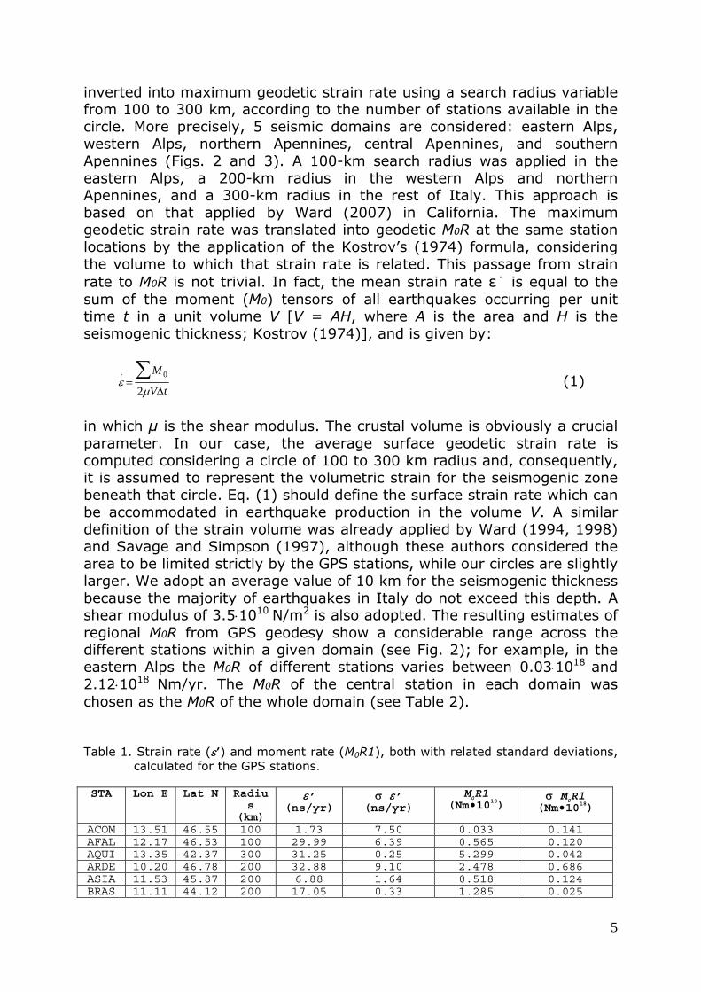
5

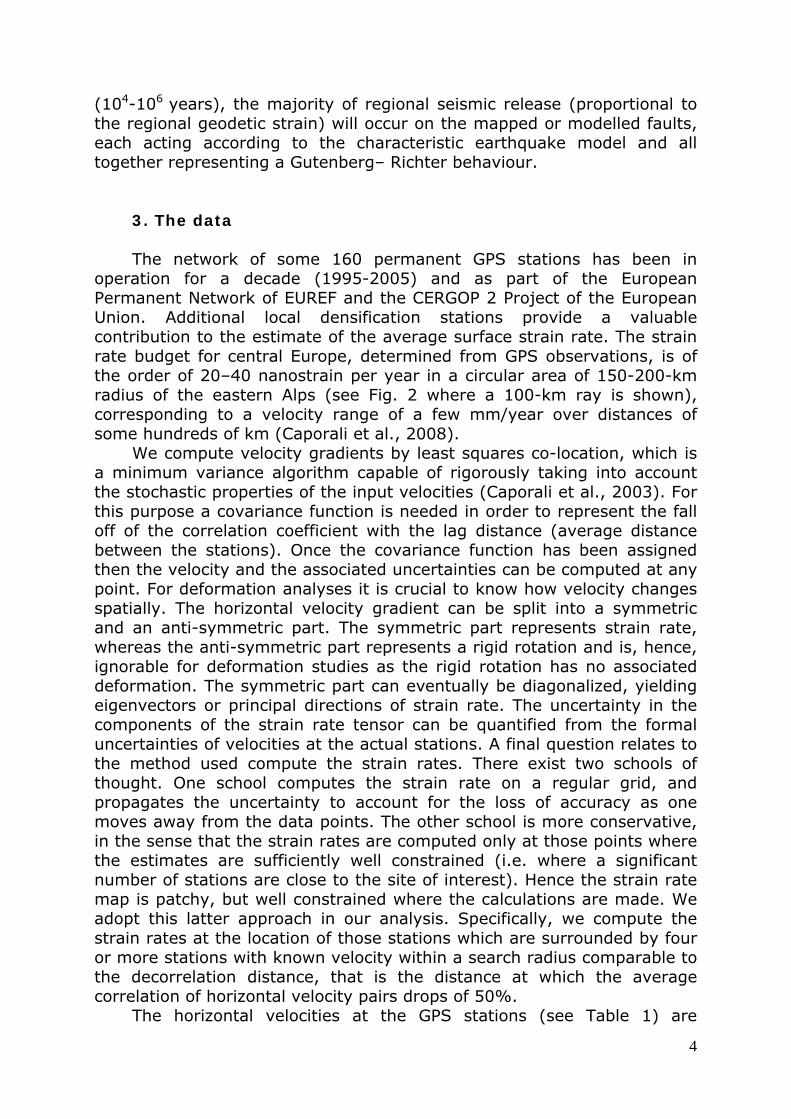
inverted into maximum geodetic strain rate using a search radius variable from 100 to 300 km, according to the number of stations available in the circle. More precisely, 5 seismic domains are considered: eastern Alps, western Alps, northern Apennines, central Apennines, and southern Apennines (Figs. 2 and 3). A 100-km search radius was applied in the eastern Alps, a 200-km radius in the western Alps and northern Apennines, and a 300-km radius in the rest of Italy. This approach is based on that applied by Ward (2007) in California. The maximum geodetic strain rate was translated into geodetic M0R at the same station locations by the application of the Kostrov’s (1974) formula, considering the volume to which that strain rate is related. This passage from strain rate to M0R is not trivial. In fact, the mean strain rate ε˙ is equal to the sum of the moment (M0) tensors of all earthquakes occurring per unit time t in a unit volume V [V = AH, where A is the area and H is the seismogenic thickness; Kostrov (1974)], and is given by:

ε.=

M 0∑2μVΔt

(1)

in which μ is the shear modulus. The crustal volume is obviously a crucial parameter. In our case, the average surface geodetic strain rate is computed considering a circle of 100 to 300 km radius and, consequently, it is assumed to represent the volumetric strain for the seismogenic zone beneath that circle. Eq. (1) should define the surface strain rate which can be accommodated in earthquake production in the volume V. A similar definition of the strain volume was already applied by Ward (1994, 1998) and Savage and Simpson (1997), although these authors considered the area to be limited strictly by the GPS stations, while our circles are slightly larger. We adopt an average value of 10 km for the seismogenic thickness because the majority of earthquakes in Italy do not exceed this depth. A shear modulus of 3.5⋅1010

N/m2 is also adopted. The resulting estimates of regional M0R from GPS geodesy show a considerable range across the different stations within a given domain (see Fig. 2); for example, in the eastern Alps the M0R of different stations varies between 0.03⋅1018

and 2.12⋅1018

Nm/yr. The M0R of the central station in each domain was chosen as the M0R of the whole domain (see Table 2).

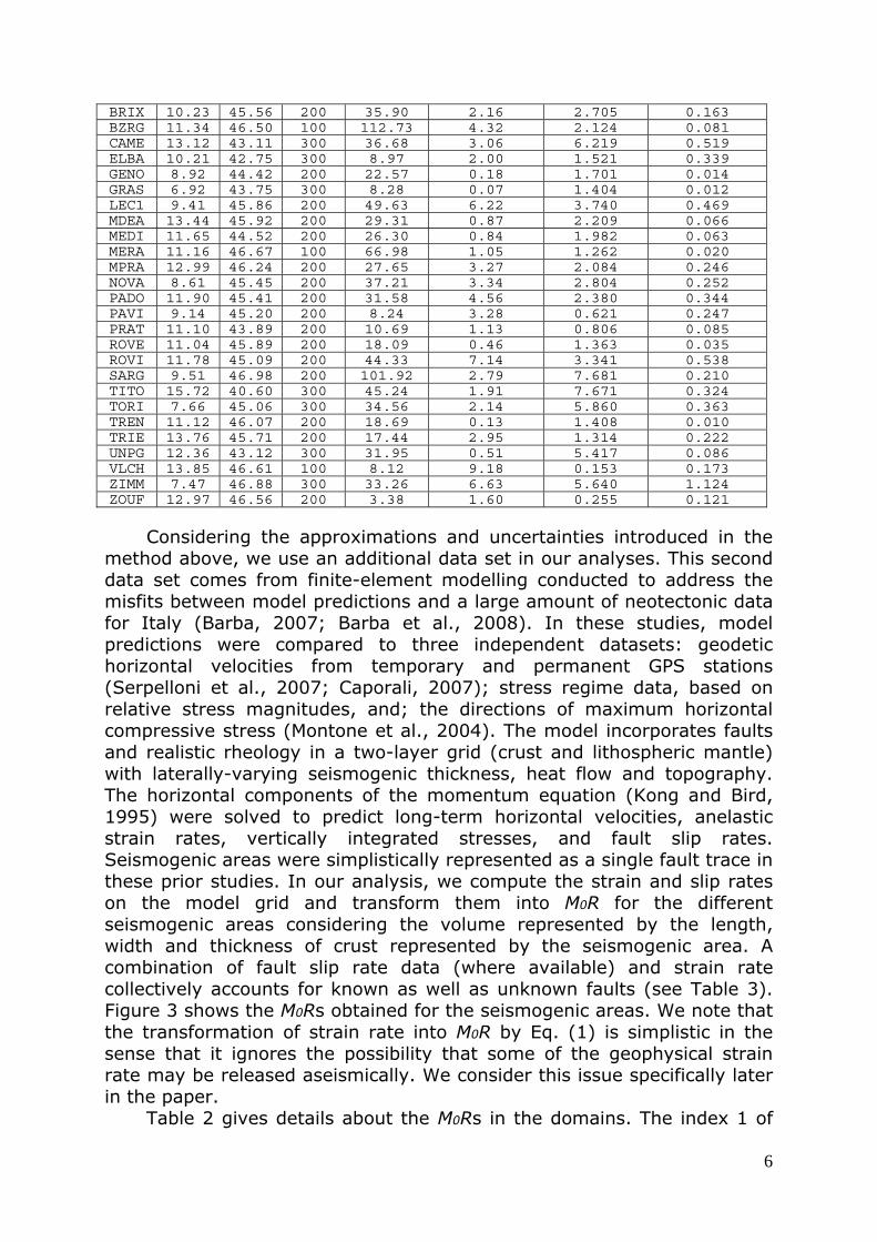
Table 1. Strain rate (ε’) and moment rate (M0R1), both with related standard deviations, calculated for the GPS stations.

STA Lon E Lat N Radiu

s (km)

ε’ (ns/yr)

σ ε’ (ns/yr)

M0R1 (Nm•1018)

σ M0R1 (Nm•1018)

ACOM 13.51 46.55 100 1.73 7.50 0.033 0.141 AFAL 12.17 46.53 100 29.99 6.39 0.565 0.120 AQUI 13.35 42.37 300 31.25 0.25 5.299 0.042 ARDE 10.20 46.78 200 32.88 9.10 2.478 0.686 ASIA 11.53 45.87 200 6.88 1.64 0.518 0.124 BRAS 11.11 44.12 200 17.05 0.33 1.285 0.025

6

BRIX 10.23 45.56 200 35.90 2.16 2.705 0.163 BZRG 11.34 46.50 100 112.73 4.32 2.124 0.081 CAME 13.12 43.11 300 36.68 3.06 6.219 0.519 ELBA 10.21 42.75 300 8.97 2.00 1.521 0.339 GENO 8.92 44.42 200 22.57 0.18 1.701 0.014 GRAS 6.92 43.75 300 8.28 0.07 1.404 0.012 LEC1 9.41 45.86 200 49.63 6.22 3.740 0.469 MDEA 13.44 45.92 200 29.31 0.87 2.209 0.066 MEDI 11.65 44.52 200 26.30 0.84 1.982 0.063 MERA 11.16 46.67 100 66.98 1.05 1.262 0.020 MPRA 12.99 46.24 200 27.65 3.27 2.084 0.246 NOVA 8.61 45.45 200 37.21 3.34 2.804 0.252 PADO 11.90 45.41 200 31.58 4.56 2.380 0.344 PAVI 9.14 45.20 200 8.24 3.28 0.621 0.247 PRAT 11.10 43.89 200 10.69 1.13 0.806 0.085 ROVE 11.04 45.89 200 18.09 0.46 1.363 0.035 ROVI 11.78 45.09 200 44.33 7.14 3.341 0.538 SARG 9.51 46.98 200 101.92 2.79 7.681 0.210 TITO 15.72 40.60 300 45.24 1.91 7.671 0.324 TORI 7.66 45.06 300 34.56 2.14 5.860 0.363 TREN 11.12 46.07 200 18.69 0.13 1.408 0.010 TRIE 13.76 45.71 200 17.44 2.95 1.314 0.222 UNPG 12.36 43.12 300 31.95 0.51 5.417 0.086 VLCH 13.85 46.61 100 8.12 9.18 0.153 0.173 ZIMM 7.47 46.88 300 33.26 6.63 5.640 1.124 ZOUF 12.97 46.56 200 3.38 1.60 0.255 0.121

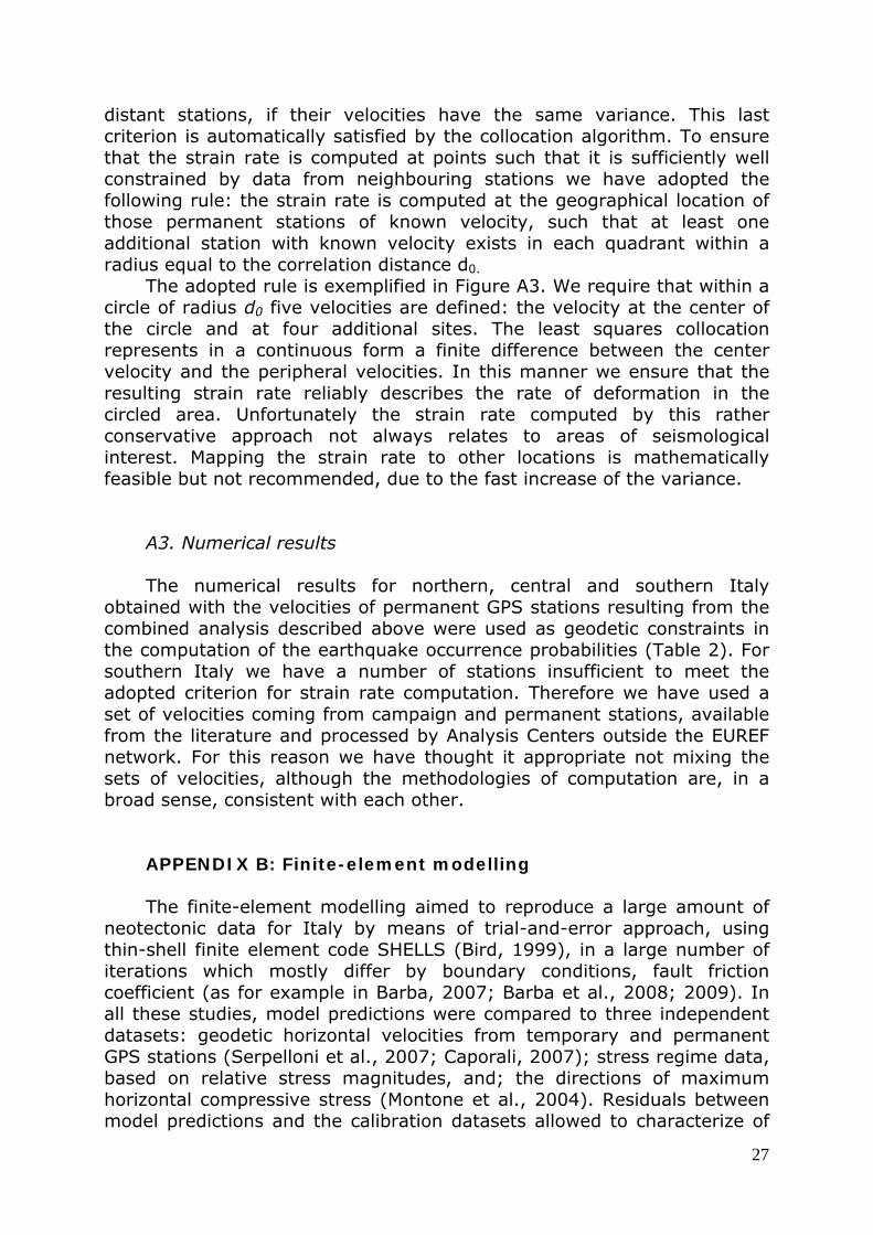
Considering the approximations and uncertainties introduced in the method above, we use an additional data set in our analyses. This second data set comes from finite-element modelling conducted to address the misfits between model predictions and a large amount of neotectonic data for Italy (Barba, 2007; Barba et al., 2008). In these studies, model predictions were compared to three independent datasets: geodetic horizontal velocities from temporary and permanent GPS stations (Serpelloni et al., 2007; Caporali, 2007); stress regime data, based on relative stress magnitudes, and; the directions of maximum horizontal compressive stress (Montone et al., 2004). The model incorporates faults and realistic rheology in a two-layer grid (crust and lithospheric mantle) with laterally-varying seismogenic thickness, heat flow and topography. The horizontal components of the momentum equation (Kong and Bird, 1995) were solved to predict long-term horizontal velocities, anelastic strain rates, vertically integrated stresses, and fault slip rates. Seismogenic areas were simplistically represented as a single fault trace in these prior studies. In our analysis, we compute the strain and slip rates on the model grid and transform them into M0R for the different seismogenic areas considering the volume represented by the length, width and thickness of crust represented by the seismogenic area. A combination of fault slip rate data (where available) and strain rate collectively accounts for known as well as unknown faults (see Table 3). Figure 3 shows the M0Rs obtained for the seismogenic areas. We note that the transformation of strain rate into M0R by Eq. (1) is simplistic in the sense that it ignores the possibility that some of the geophysical strain rate may be released aseismically. We consider this issue specifically later in the paper.

Table 2 gives details about the M0Rs in the domains. The index 1 of

7

the Table refers to the GPS observations, while the index 2 refers to the results of the geophysical modelling. In the case of the geodetic constraint, the domain M0R (M0R1 in Table 2) corresponds to that calculated for the central GPS station and represents the sum of the M0R of each seismogenic area in the domain, plus the M0R of the distributed seismicity (earthquakes of MW less than 5.5 and, consequently, outside the seismogenic areas), plus that released as aseismic creep. In the case of the geophysical constraint, the domain M0R (M0R2 in Table 2) is given by the sum of the M0Rs of the seismogenic areas calculated by the geophysical modelling. In the case of the geodetic constraint, the number of seismogenic areas inside the search circle (SAN1 in Table 2) can be larger than the actual number of seismogenic areas inside the domain because the same seismogenic area can belong to more than one domain if it is located in the overlapping areas of search circles. As it was not possible to compute the M0R by the geophysical modelling for all the seismogenic areas, the number of seismogenic areas inside a domain in the case of the geophysical constraint (SAN2 in Table 2) can be less than the actual number of seismogenic areas inside that domain defined in the Italian Seismogenic Source Database. This explains the differences between the numbers in Table 2 and what shown by Figures 2 and 3.

Table 2. M0Rs of the domains. The index 1 refers to the GPS observations, while the

index 2 refers to the results of the geophysical modelling. M0R 1 is computed for the reference station while M0R 2 is given by the sum of the M0Rs calculated by modelling for the seismogenic areas belonging to each domain. SAN1 represents the number of seismogenic areas inside the search circle and can be larger than the actual number of seismogenic areas inside the domain (the same seismogenic area can belong to more than one domain if it is located in the overlapping areas of search circles). SAN2 is the number of seismogenic areas inside the domain for which M0R was possible to compute by the geophysical modelling (no overlapping areas as the seismogenic areas are associated to the pertinent domain only).

Domain Reference

station Search

ray (km) SAN1 M0R1

(N⋅m/yr) SAN2 M0R2

(N⋅m/yr) E Alps Faloria 100 10 0.56⋅1018 5 1.01⋅1017 W Alps Pavia 200 20 0.62⋅1018 4 1.53⋅1017

N Apennines Medicina 200 47 1.98⋅1018 18 3.29⋅1017 S Apennines Tito 300 34 7.67⋅1018 26 4.77⋅1017 Table 3. Strain rate (ε’) and moment rate (M0R2), modelled for the seismogenic areas.

Source Region Lon Lat ε’

(ns/yr) M0R2

(Nm•1015) ITSA002 Cent._South._Alps 9.859 45.460 0.90 6.554 ITSA003 Ripabottoni 15.029 41.685 1.60 1.544 ITSA004 Ascoli_Satriano 15.677 41.309 1.40 2.450 ITSA005 Picerno-Massafra 16.328 40.634 21.40 7.068 ITSA006 Sciacca-Gela 13.374 37.407 4.00 5.314 ITSA008 Conero_onshore 13.668 43.506 7.80 6.391 ITSA010 Copparo-Comacchio 12.035 44.743 5.90 7.420 ITSA012 Portomaggiore 12.001 44.629 5.40 7.486

8

ITSA013 Aremogna 14.037 41.822 30.60 16.483 ITSA014 South._Tyrrhenian 14.072 38.460 6.90 53.857 ITSA015 Crati_Valley 16.285 39.186 45.20 55.998 ITSA016 Aspromonte 15.516 38.133 118.90 16.699 ITSA017 Scicli-Catania 14.908 37.161 57.90 79.656 ITSA019 Crotone_-_Rossano 17.022 39.287 14.60 11.859 ITSA020 Southern_Marche 13.523 43.229 13.50 46.704 ITSA021 Marsala-Belice 12.921 37.764 5.30 2.142 ITSA024 Castelpetroso 14.487 41.468 51.30 60.454 ITSA025 In_C._Apennines 13.166 42.543 29.10 49.059 ITSA027 Out_C._Apennines 12.401 43.630 12.50 30.959 ITSA028 Colfiorito 12.889 43.024 81.60 15.391 ITSA029 Gela-Catania 14.577 37.324 63.60 28.045 ITSA031 Conero_offshore 13.687 43.578 7.50 8.296 ITSA032 Pesaro-Senigallia 13.251 43.650 4.00 18.134 ITSA033 Mt._Pollino_South 16.215 39.809 22.40 8.153 ITSA034 Irpinia 15.464 40.663 37.40 54.261 ITSA035 Ragusa-Palagonia 14.766 37.151 13.90 18.460 ITSA037 Mugello 11.237 44.004 23.60 4.128 ITSA038 Mercure_Basin 15.929 40.015 39.70 25.133 ITSA040 Castelluccio 13.350 42.561 28.40 57.716 ITSA041 Selci_Lama 12.226 43.502 37.60 8.261 ITSA042 Patti-Eolie 14.974 38.298 30.40 9.523 ITSA043 Pesaro-Senigallia 13.019 43.955 7.00 10.580 ITSA051 Mirandola 11.354 44.801 3.10 4.685 ITSA053 Southern_Calabria 16.220 38.616 79.70 37.045 ITSA054 Porto_San_Giorgio 13.924 42.889 13.70 8.434 ITSA055 Bagnara 15.928 38.233 15.70 15.197 ITSA056 Gubbio_Basin 12.611 43.210 59.40 23.835 ITSA057 Pago_Veiano 15.163 41.238 7.30 2.808 ITSA058 Mattinata 15.830 41.710 1.30 0.969 ITSA059 Tremiti 14.757 42.180 2.20 5.313 ITSA060 Montello 12.202 45.864 15.90 4.273 ITSA061 Cansiglio 12.558 46.117 16.20 8.883 ITSA062 Maniago-Sequals 12.850 46.202 14.60 25.187 ITSA063 Andretta-Filano 15.415 40.874 49.10 26.406 ITSA064 Tramonti-Kobarid 13.378 46.294 11.70 33.937 ITSA066 Gemona-Tarcento 13.265 46.210 28.20 19.751 ITSA068 Catanzaro_Trough 16.365 38.861 30.22 24.122 ITSA075 Pietracamela 13.704 42.487 9.50 5.804 ITSA077 Pescolanciano 14.594 41.654 52.10 2.968 ITSA079 Campomarino 14.612 41.986 4.30 6.424 ITSA080 Nicotera- 16.162 38.431 45.00 6.407 ITSA084 Vallata 15.442 41.058 11.50 3.155 ITSA087 Conza -Tolve 15.393 40.840 67.10 22.212 ITSA089 Melfi-Spinazzola 16.036 40.969 1.70 0.972 SISA002 Tolmin-Idrija 14.176 45.918 29.70 15.373

Figure 2 displays the M0Rs calculated for the GPS stations from the

geodetic observations (circles): the squares highlight the reference stations, whose M0Rs are associated to the domain (M0R1 in Table 2) and used as input data in the following computations. The circles in Figure 3 quantify the M0R computed by the geophysical modelling for each seismogenic area: the sum of the M0Rs inside each domain gives the value reported in Table 2 (M0R2). A direct comparison between the M0R estimates obtained with the two different methods is not possible. In fact, according to the geodetic constraints, the value reported in Table 2 overestimates the M0R of the domain because some seismogenic areas are counted more than once as they appear in several domains, depending on the overlapping of the search radii. According to the

9

geophysical constraints, the value reported in Table 2 underestimates the M0R of the domain because it is not possible to compute the strain rate (and, consequently, the M0R) for all the seismogenic areas by the geophysical modelling. The two estimates differ by a factor from 5 to 12, and those calculated with geodetic constraints are higher than those computed by the geophysical modelling (see Table 2). This discrepancy is motivated by the fact that the M0R in each domain from GPS observations is given by the sum of the M0R released as characteristic earthquakes plus that released as distributed seismicity and as aseismic creep, while the M0R from geophysical modelling refers only to the contribution of the characteristic earthquakes.

4. Comparison of moment rate derived from geodetic and seismicity data

To compare the observed geodetic moment rate (M0R1) with the

seismic one, domain catalogues have been extracted from the Italian earthquake catalogue (Gruppo di Lavoro CPTI, 2004). These catalogues collect all the events in a circle centred on the reference GPS stations (Faloria, Pavia, Medicina, Tito) and with the same radius as that used for the computation of M0R1: 100 km for Faloria, 200 km for Pavia and Medicina, and 300 km for Tito. The observed seismic moment rate (M0Ross) in each of the four domains has been computed considering all the earthquakes which have occurred since the beginning of the 18th century, because this period can be considered complete for MW 5.5 and over. The Hanks and Kanamori (1979) relation was used to compute seismic moment from MW and the observed seismic moment rate of events with MW 5.5 and over (M0Ross5.5) was computed as well (Fig. 4).

As the above M0Ross does not represent the total seismic moment rate, the Gutenberg– Richter relation was calculated for the four domains. First, the seismicity rates for each magnitude class were computed by the Albarello and Mucciarelli (2002) approach, where the whole catalogue is divided into time intervals for each of which the probability that it is complete is evaluated and the related rate is weighted accordingly. The Gutenberg– Richter parameters (a- and b-values) were calculated by the application of the maximum likelihood approach according to the Weichert (1980) procedure. From the Gutenberg – Richter distribution, the individual annual rates were derived and, from them and the MWs (from the maximum observed magnitude to 0.1), the calculated seismic moment rate (M0Rcal) was obtained. As this M0Rcal was calculated considering all the MWs, it should represent the actual seismic moment rate released by each domain. In addition, the computed seismic moment rate for events with MW 5.5 and over (M0Rcal5.5) was also computed. It can be seen from Table 4, where all the results are reported, that the M0Rcal is larger than the M0Ross and the difference varies from one domain to the other from less than two times in the eastern Alps to more than three times in the western Alps. It is notable the situation of the southern Apennines, where

10

M0Ross is larger than M0Rcal because of the large number of moderate-to-large earthquakes which occurred there in the last three centuries. Increasing the time period over which the calculation is done the value of M0Ross decreases notably (e.g.: it is 12.0⋅1017 when calculated considering the last 5 centuries). Moreover, it is quite interesting to observe which is the contribution in terms of calculated seismic moment rate given by the strong earthquakes (MW 5.5 and over) in each domain. Also in this case the ratio spans over a large interval: large earthquakes contribute largely in the eastern Alps and in the southern Apennines, where their presence is frequent, while their contribution is limited in the other two domains.

The final comparison refers to the ratio between M0Rcal and M0R1 and quantifies the amount of strain which is supposed to be released seismically. This ratio is quite constant around 20-30% with the exception of the western Alps, where it is about 60%. Bressan and Bragato (2009) have found that a significant part of deformation occurs aseismically in the eastern Alps.

B3 In summary, the comparison among the 3 estimates of M0R shows that: 1) M0Rcal is much larger than M0Ross, with the exception of the southern Apennines; 2) M0R1 is larger (about double) than M0Rcal, with the exception of the western Alps. These values will be introduced in the following computations. More precisely, the part of the M0R which is supposed to be released aseismically (obtained from M0Rcal/M0R1 in Table 4) will be subtracted from M0R1 in the analysis referring to the domains. The ratio between total moment rate from the finite element model and the seismic moment rate for Mw>=5.5 is 1.06. Thus, such correction is applied, subtracting 6% from M0R2 in the analysis referring to the seismogenic areas. The M0R referring to the distributed seismicity (events with an MW<5.5), which is not considered in M0R2 (Barba, personal communication), can be calculated from the ratio between the M0R released by large and all earthquakes (M0Rcal5.5/M0Rcal in Table 4) and it is added to M0R2 before the computations. Conversely, M0R1 does not need any addiction, as it is comprehensive of the earthquakes of all magnitude.

As the geophysical model is satisfactorily constrained only for the Apennines, we will restrict the following elaborations only to the seismogenic areas along the Apennines. Table 4. Annual moment rates (in N⋅m/yr) and b-values (with related standard deviation)

for the four domains. M0R1 is the geodetic value (see Table 2), M0Ross is the value observed in the last 3 centuries according to the Italian earthquake catalogue (Gruppo di lavoro CPTI, 2004), M0Ross5.5 is the same as M0Ross but referring to earthquakes with an MW 5.5 and over, M0Rcal is the value calculated from the Gutenberg– Richter relation for all MW, M0Rcal5.5 is the same as M0Rcal but calculated for earthquakes with an MW 5.5 and over.

Domain b-

value σb M

0R1

(⋅1017) M0R

oss

(⋅1017) M

0R

oss5.5

(⋅1017) M0Rcal

(⋅1017) M0Rcal5.5

(⋅1017)

M0Rcal5.5

/M

0Rcal

M

0R

cal

/M0R1

E Alps 1.13 0.15 5.6 0.62 0.49 1.17 0.85 0.73 0.21 W Alps 1.50 0.13 6.2 1.07 0.69 3.89 0.70 0.18 0.63 N Apen. 1.44 0.10 19.8 1.93 1.35 5.33 1.63 0.31 0.27

11

S Apen. 1.09 0.06 76.7 15.7 14.9 14.5 9.37 0.85 0.19

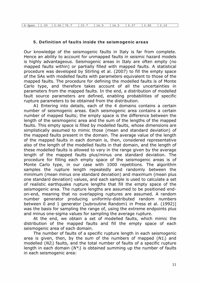
5. Definition of faults inside the seismogenic areas

Our knowledge of the seismogenic faults in Italy is far from complete. Hence an ability to account for unmapped faults in seismic hazard models is highly advantageous. Seismogenic areas in Italy are often empty (no mapped faults within) or partially filled with mapped faults. A statistical procedure was developed by Stirling et al. (2007) to fill the empty space of the SAs with modelled faults with parameters equivalent to those of the mapped faults. The procedure for defining the modelled faults is of Monte Carlo type, and therefore takes account of all the uncertainties in parameters from the mapped faults. In the end, a distribution of modelled fault source parameters are defined, enabling probabilities of specific rupture parameters to be obtained from the distribution.

A1 Entering into details, each of the 4 domains contains a certain number of seismogenic areas. Each seismogenic area contains a certain number of mapped faults; the empty space is the difference between the length of the seismogenic area and the sum of the lengths of the mapped faults. This empty space is filled by modelled faults, whose dimensions are simplistically assumed to mimic those (mean and standard deviation) of the mapped faults present in the domain. The average value of the length of the mapped faults in each domain is, then, considered representative also of the length of the modelled faults in that domain, and the length of these modelled faults is allowed to vary in the range given by the average length of the mapped faults plus/minus one standard deviation. The procedure for filling each empty space of the seismogenic areas is of Monte Carlo type, in our case with 1000 repetitions. The algorithm samples the rupture length repeatedly and randomly between the minimum (mean minus one standard deviation) and maximum (mean plus one standard deviation) values, and each sample is used to calculate a set of realistic earthquake rupture lengths that fill the empty space of the seismogenic area. The rupture lengths are assumed to be positioned end-on-end, meaning that no overlapping ruptures are assumed. A random number generator producing uniformly-distributed random numbers between 0 and 1 generator [subroutine Random1 in Press et al. (1992)] was the basis for sampling the range of, using the extreme endpoints plus and minus one-sigma values for sampling the average rupture.

At the end, we obtain a set of modelled faults, which mimic the distribution of the mapped faults and fill the empty space of each seismogenic area of each domain.

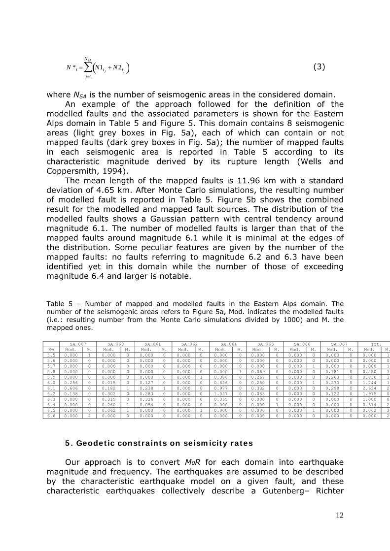
The number of faults of a specific rupture length in each seismogenic area is given, then, by the sum of the numbers of mapped (N1i) and modelled (N2i) faults, and the total number of faults of a specific rupture length in each domain (N*i) is obtained summing up the number of faults in each seismogenic area:

12

N *i = N1i j+ N2i j( )

j=1

NSA

∑ (3)

where NSA is the number of seismogenic areas in the considered domain.

An example of the approach followed for the definition of the modelled faults and the associated parameters is shown for the Eastern Alps domain in Table 5 and Figure 5. This domain contains 8 seismogenic areas (light grey boxes in Fig. 5a), each of which can contain or not mapped faults (dark grey boxes in Fig. 5a); the number of mapped faults in each seismogenic area is reported in Table 5 according to its characteristic magnitude derived by its rupture length (Wells and Coppersmith, 1994).

The mean length of the mapped faults is 11.96 km with a standard deviation of 4.65 km. After Monte Carlo simulations, the resulting number of modelled fault is reported in Table 5. Figure 5b shows the combined result for the modelled and mapped fault sources. The distribution of the modelled faults shows a Gaussian pattern with central tendency around magnitude 6.1. The number of modelled faults is larger than that of the mapped faults around magnitude 6.1 while it is minimal at the edges of the distribution. Some peculiar features are given by the number of the mapped faults: no faults referring to magnitude 6.2 and 6.3 have been identified yet in this domain while the number of those of exceeding magnitude 6.4 and larger is notable.

Table 5 – Number of mapped and modelled faults in the Eastern Alps domain. The number of the seismogenic areas refers to Figure 5a, Mod. indicates the modelled faults (i.e.: resulting number from the Monte Carlo simulations divided by 1000) and M. the mapped ones. SA_007 SA_060 SA_061 SA_062 SA_064 SA_065 SA_066 SA_067 Tot. Mw Mod. M. Mod. M. Mod. M. Mod. M. Mod. M. Mod. M. Mod. M. Mod. M. Mod. M.5.5 0.000 1 0.000 0 0.000 0 0.000 0 0.000 0 0.000 0 0.000 0 0.000 0 0.000 15.6 0.000 0 0.000 0 0.000 0 0.000 0 0.000 0 0.000 0 0.000 0 0.000 0 0.000 05.7 0.000 0 0.000 0 0.000 0 0.000 0 0.000 0 0.000 0 0.000 1 0.000 0 0.000 15.8 0.000 0 0.000 0 0.000 0 0.000 0 0.000 1 0.069 0 0.000 0 0.181 0 0.250 15.9 0.000 0 0.000 0 0.000 0 0.000 1 0.306 0 0.267 0 0.000 0 0.263 0 0.836 16.0 0.256 0 0.015 0 0.127 0 0.000 0 0.826 0 0.250 0 0.000 1 0.270 0 1.744 16.1 0.606 0 0.182 1 0.238 1 0.000 0 0.977 0 0.332 0 0.000 0 0.299 0 2.634 26.2 0.138 0 0.302 0 0.283 0 0.000 0 1.047 0 0.083 0 0.000 0 0.122 0 1.975 06.3 0.000 0 0.319 0 0.326 0 0.000 0 0.355 0 0.000 0 0.000 0 0.000 0 1.000 06.4 0.000 0 0.260 1 0.054 0 0.000 0 0.000 0 0.000 1 0.000 0 0.000 0 0.314 26.5 0.000 0 0.062 1 0.000 0 0.000 1 0.000 0 0.000 0 0.000 1 0.000 0 0.062 36.6 0.000 2 0.000 0 0.000 0 0.000 0 0.000 0 0.000 0 0.000 0 0.000 0 0.000 2

5. Geodetic constraints on seismicity rates Our approach is to convert M0R for each domain into earthquake

magnitude and frequency. The earthquakes are assumed to be described by the characteristic earthquake model on a given fault, and these characteristic earthquakes collectively describe a Gutenberg– Richter

13

distribution at a regional scale (i.e. within each domain, or Italy as a whole). We also calculate distributed earthquake recurrence parameters for each domain from a combination of catalogue seismicity and geodetic observations. Gutenberg-Richter b-values of each domain are computed from the seismicity observed in the domain itself, while the a-value of each domain can be obtained from the geodetic observations, i.e. from the M0R in the domain. In fact, logN = a'−b'logM0 (4) where N is the number of earthquakes with seismic moment larger than, or equal to, M0, where

a'= a +9.11.5

b (5)

and

b'= 11.5

b (6)

considering the relation between magnitude, MW, and M0 in Nm (Hanks and Kanamori, 1979): log M0 = 9.1+1.5MW (7)

Knowing the value of the M0R in the domain under study, in our case obtained from the geodetic observations, and fixing the maximum value for M0, derived from the maximum magnitude for that domain, we can write: M 0R = Ni

i∑ M 0i

(8)

where Ni is the unknown annual non-cumulative number of earthquakes with M0i, and the index i represents all the classes of M0 in the domain. From Eq. (4) we have

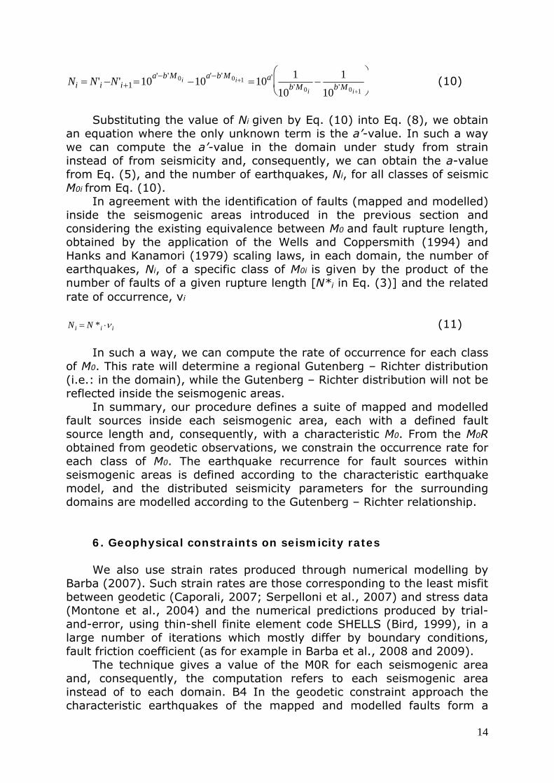
N 'i =10a'−b'M 0i (9) where N’i is the cumulative number of earthquakes with M0i and above. From the cumulative number we can compute the non-cumulative number Ni:

14

Ni = N'i −N'i+1=10a'−b'M 0i −10a'−b'M 0i+1 =10a' 110b'M 0i

−1

10b'M 0i+1

⎛

⎝ ⎜

⎞

⎠ ⎟ (10)

Substituting the value of Ni given by Eq. (10) into Eq. (8), we obtain

an equation where the only unknown term is the a’-value. In such a way we can compute the a’-value in the domain under study from strain instead of from seismicity and, consequently, we can obtain the a-value from Eq. (5), and the number of earthquakes, Ni, for all classes of seismic M0i from Eq. (10).

In agreement with the identification of faults (mapped and modelled) inside the seismogenic areas introduced in the previous section and considering the existing equivalence between M0 and fault rupture length, obtained by the application of the Wells and Coppersmith (1994) and Hanks and Kanamori (1979) scaling laws, in each domain, the number of earthquakes, Ni, of a specific class of M0i is given by the product of the number of faults of a given rupture length [N*i in Eq. (3)] and the related rate of occurrence, νi

Ni = N *i ⋅ν i (11)

In such a way, we can compute the rate of occurrence for each class of M0. This rate will determine a regional Gutenberg – Richter distribution (i.e.: in the domain), while the Gutenberg – Richter distribution will not be reflected inside the seismogenic areas.

In summary, our procedure defines a suite of mapped and modelled fault sources inside each seismogenic area, each with a defined fault source length and, consequently, with a characteristic M0. From the M0R obtained from geodetic observations, we constrain the occurrence rate for each class of M0. The earthquake recurrence for fault sources within seismogenic areas is defined according to the characteristic earthquake model, and the distributed seismicity parameters for the surrounding domains are modelled according to the Gutenberg – Richter relationship.

6. Geophysical constraints on seismicity rates We also use strain rates produced through numerical modelling by

Barba (2007). Such strain rates are those corresponding to the least misfit between geodetic (Caporali, 2007; Serpelloni et al., 2007) and stress data (Montone et al., 2004) and the numerical predictions produced by trial-and-error, using thin-shell finite element code SHELLS (Bird, 1999), in a large number of iterations which mostly differ by boundary conditions, fault friction coefficient (as for example in Barba et al., 2008 and 2009).

The technique gives a value of the M0R for each seismogenic area and, consequently, the computation refers to each seismogenic area instead of to each domain. B4 In the geodetic constraint approach the characteristic earthquakes of the mapped and modelled faults form a

15

Gutenberg – Richter distribution in the domains but not necessarily inside the seismogenic areas. Differently, in the geophysical constraint approach, the characteristic earthquakes of the mapped and modelled fault sources defined inside each seismogenic area collectively define a Gutenberg – Richter distribution. The observation of a Gutenberg – Richter distribution for large regions, countries and the globe is well documented (e.g. WGCEP, 1995; Stirling et al., 1996).

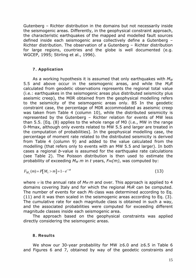
7. Application As a working hypothesis it is assumed that only earthquakes with MW

5.5 and above occur in the seismogenic areas, and while the M0R calculated from geodetic observations represents the regional total value (i.e.: earthquakes in the seismogenic areas plus distributed seismicity plus aseismic creep), the M0R obtained from the geophysical modelling refers to the seismicity of the seismogenic areas only. B5 In the geodetic constraint case, the percentage of M0R accommodated as aseismic creep was taken from Table 4 (column 10), while the distributed seismicity is represented by the Gutenberg – Richter relation for events of MW less than 5.5. [Eq. (8) applies to the whole range of M0 (i.e., MW in the range 0-Mmax, although only events related to MW 5.5 and larger are treated in the computation of probabilities]. In the geophysical modelling case, the percentage of moment rate related to the distributed seismicity is derived from Table 4 (column 9) and added to the value calculated from the modelling (that refers only to events with an MW 5.5 and larger). In both cases a regional b-value is assumed for the earthquake rate calculations (see Table 2). The Poisson distribution is then used to estimate the probability of exceeding MW m in t years, FMt(m), was computed by: FM t

(m) = P Mt > m[ ]=1− e−νt (13)

where ν is the annual rate of MW m and over. This approach is applied to 4 domains covering Italy and for which the regional M0R can be computed. The number of events for each M0 class was determined according to Eq. (11) and it was then scaled in the seismogenic areas according to Eq. (3). The cumulative rate for each magnitude class is obtained in such a way, and the associated probabilities were computed for exceeding different magnitude classes inside each seismogenic area.

The approach based on the geophysical constraints was applied directly considering the seismogenic areas.

8. Results We show our 30-year probability for MW ≥6.0 and ≥6.5 in Table 6

and Figures 6 and 7, obtained by way of the geodetic constraints and

16

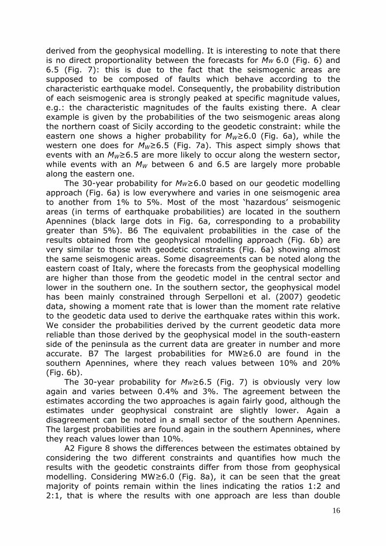
derived from the geophysical modelling. It is interesting to note that there is no direct proportionality between the forecasts for MW 6.0 (Fig. 6) and 6.5 (Fig. 7): this is due to the fact that the seismogenic areas are supposed to be composed of faults which behave according to the characteristic earthquake model. Consequently, the probability distribution of each seismogenic area is strongly peaked at specific magnitude values, e.g.: the characteristic magnitudes of the faults existing there. A clear example is given by the probabilities of the two seismogenic areas along the northern coast of Sicily according to the geodetic constraint: while the eastern one shows a higher probability for MW≥6.0 (Fig. 6a), while the western one does for MW≥6.5 (Fig. 7a). This aspect simply shows that events with an MW≥6.5 are more likely to occur along the western sector, while events with an MW between 6 and 6.5 are largely more probable along the eastern one.

The 30-year probability for MW≥6.0 based on our geodetic modelling approach (Fig. 6a) is low everywhere and varies in one seismogenic area to another from 1% to 5%. Most of the most ‘hazardous’ seismogenic areas (in terms of earthquake probabilities) are located in the southern Apennines (black large dots in Fig. 6a, corresponding to a probability greater than 5%). B6 The equivalent probabilities in the case of the results obtained from the geophysical modelling approach (Fig. 6b) are very similar to those with geodetic constraints (Fig. 6a) showing almost the same seismogenic areas. Some disagreements can be noted along the eastern coast of Italy, where the forecasts from the geophysical modelling are higher than those from the geodetic model in the central sector and lower in the southern one. In the southern sector, the geophysical model has been mainly constrained through Serpelloni et al. (2007) geodetic data, showing a moment rate that is lower than the moment rate relative to the geodetic data used to derive the earthquake rates within this work. We consider the probabilities derived by the current geodetic data more reliable than those derived by the geophysical model in the south-eastern side of the peninsula as the current data are greater in number and more accurate. B7 The largest probabilities for MW≥6.0 are found in the southern Apennines, where they reach values between 10% and 20% (Fig. 6b).

The 30-year probability for MW≥6.5 (Fig. 7) is obviously very low again and varies between 0.4% and 3%. The agreement between the estimates according the two approaches is again fairly good, although the estimates under geophysical constraint are slightly lower. Again a disagreement can be noted in a small sector of the southern Apennines. The largest probabilities are found again in the southern Apennines, where they reach values lower than 10%.

A2 Figure 8 shows the differences between the estimates obtained by considering the two different constraints and quantifies how much the results with the geodetic constraints differ from those from geophysical modelling. Considering MW≥6.0 (Fig. 8a), it can be seen that the great majority of points remain within the lines indicating the ratios 1:2 and 2:1, that is where the results with one approach are less than double

17

those with the other approach. There are a few among the remaining points where the estimates with geodetic constraints are by far larger (more than 4 times) than those from geophysical modelling. The situation is worse when events with an MW≥6.5 are considered (Fig. 8b). In this case almost all forecasts with geodetic constraints are larger than those from geophysical modelling and even values larger 10 times and more are obtained in a few cases.

The only region where the estimates with the two approaches, referring to MW≥6.0 and MW≥6.5 as well, differ largely is the promontory in the southern Adriatic sea (Gargano promontory). There, the forecasts from the geophysical modelling are much lower than those with geodetic constraints: this difference is notably larger than that in the rest of Italy.

Some explanations for the differences shown by the two approaches can be suggested. Both methods suffer some limitations: the geodetic one because it was possible to compute the strain rate over wide regions (the 4 domains, see Appendix A) and some peculiar differences are, consequently, lost. The geophysical modelling is not yet tuned perfectly and a satisfactory agreement with all the boundary conditions is not reached yet (see Appendix B).

The lack of proportionality between the estimates referring to a different magnitude threshold has been already justified, and is more evident in the case of a geodetic constraint (Fig. 8c) than when data from the geophysical modelling have been used (Fig. 8d). These latter, in fact, display quite a nice alignment along the line 10:1, indicating that the probability of MW≥6.0 is about 10 times larger than that of MW≥6.5.

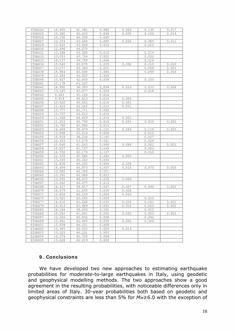
Table 6 – Exceedence probability in 30 years for magnitude 6.0 and 6.5. P1 indicates the results obtained with geodetic constraints, P2 those with geophysical constraints. The name of the seismogenic areas (SA_ID) is made up of the country code (CH for Switzerland, FR for France, IT for Italy, SI for Slovenia) followed by SA, and the code number of the seismogenic area.

SA_ID Lon. Lat. P1-6.0 P1-6.5 P2-6.0 P2-6.5 CHSA001 7.974 46.301 0.014 CHSA002 7.255 46.117 0.013 FRSA001 6.655 44.706 0.013 ITSA001 11.826 44.231 0.010 0.001 ITSA002 9.820 45.438 0.014 0.003 0.011 0.001 ITSA003 15.161 41.699 0.080 0.031 0.003 0.001 ITSA004 15.965 41.287 0.177 0.002 0.007 ITSA005 16.333 40.642 0.051 0.013 ITSA007 11.690 45.766 0.031 0.014 ITSA008 13.578 43.541 0.007 0.009 ITSA009 10.270 44.824 0.014 0.001 ITSA010 12.035 44.743 0.015 0.002 ITSA011 12.045 44.348 0.011 ITSA012 12.080 44.567 0.014 0.001 0.015 0.002 ITSA013 13.975 41.870 0.035 0.023 ITSA014 13.180 38.339 0.039 0.036 0.085 0.027 ITSA015 16.249 39.375 0.113 0.097 ITSA016 15.599 38.103 0.030 0.030 0.007 0.007 ITSA018 9.146 44.997 0.014 0.001 ITSA019 17.016 39.294 0.035 0.025 0.035 0.006 ITSA020 13.664 42.990 0.010 0.084 ITSA022 7.767 43.880 0.022 0.001 ITSA023 7.385 44.890 0.011

18

ITSA024 14.605 41.382 0.085 0.054 0.130 0.017 ITSA025 13.382 42.263 0.044 0.035 0.100 0.014 ITSA026 10.150 44.299 0.040 ITSA027 12.374 43.684 0.080 0.026 0.085 0.011 ITSA028 12.835 43.069 0.024 0.022 ITSA030 12.696 44.073 ITSA031 13.698 43.580 0.010 0.015 ITSA032 13.053 43.754 0.021 0.030 ITSA033 16.237 39.789 0.048 0.016 ITSA034 15.540 40.575 0.215 0.092 0.210 0.020 ITSA037 12.277 43.384 0.021 0.008 0.001 ITSA038 15.954 40.040 0.086 0.099 0.004 ITSA039 12.494 44.047 0.009 ITSA040 13.427 42.460 0.039 0.103 ITSA041 12.178 43.547 ITSA042 14.990 38.309 0.094 0.029 0.033 0.004 ITSA043 13.145 43.877 0.009 0.018 ITSA044 9.643 45.124 0.014 ITSA045 9.919 44.815 0.014 0.005 ITSA046 10.520 44.561 0.014 0.001 ITSA047 11.424 44.425 0.014 0.001 ITSA048 10.777 45.771 0.022 ITSA049 10.727 44.810 0.015 ITSA050 11.508 44.869 0.014 0.001 ITSA051 11.212 44.794 0.014 0.001 0.010 0.001 ITSA052 14.780 42.946 0.010 ITSA053 16.099 38.479 0.131 0.044 0.116 0.022 ITSA054 13.898 43.016 0.008 0.012 ITSA055 15.918 38.228 0.140 0.027 ITSA056 12.493 43.279 0.041 0.026 ITSA057 15.040 41.243 0.064 0.064 0.001 0.001 ITSA058 15.837 41.717 0.149 0.003 ITSA059 14.750 42.179 0.137 0.010 ITSA060 12.330 45.982 0.046 0.005 ITSA061 13.240 46.262 0.036 ITSA062 12.836 46.205 0.004 0.004 ITSA063 15.494 40.873 0.037 0.015 0.073 0.010 ITSA064 13.082 46.306 0.021 ITSA065 13.391 45.969 0.023 ITSA066 13.255 46.215 0.032 0.004 ITSA067 13.042 46.477 0.013 ITSA068 16.357 38.817 0.047 0.007 0.044 0.003 ITSA070 16.579 41.635 0.036 0.028 ITSA071 12.806 46.218 0.004 0.004 ITSA075 13.925 42.492 0.009 0.010 ITSA077 14.510 41.660 0.030 0.030 0.001 0.001 ITSA079 14.613 41.989 0.042 0.012 0.022 0.002 ITSA080 16.164 38.434 0.141 0.012 ITSA084 15.302 41.041 0.052 0.052 0.003 0.003 ITSA087 15.356 40.855 0.048 0.044 ITSA089 15.881 40.969 0.095 0.002 0.004 SISA001 13.838 46.201 0.008 SISA002 13.945 46.055 0.024 0.014 SISA003 13.525 46.291 0.003 SISA004 14.074 45.705 0.008 SISA005 13.628 46.019 0.009

9. Conclusions We have developed two new approaches to estimating earthquake

probabilities for moderate-to-large earthquakes in Italy, using geodetic and geophysical modelling methods. The two approaches show a good agreement in the resulting probabilities, with noticeable differences only in limited areas of Italy. 30-year probabilities both based on geodetic and geophysical constraints are less than 5% for MW≥6.0 with the exception of

19

the southern Apennines, where they reach values between 10% and 20% in a very few seismogenic areas. In the same areas, 30-year probabilities for MW≥6.5 remain lower than 10%. Future work will be focussed on improving the methodologies developed, in an effort to constrain better the derived earthquake probabilities.

Acknowledgements. The present study has been developed in the

framework of the projects of interest for the Italian Department of Civil Protection and financed by the National Institute of Geophysics and Volcanology. Many thanks are due to Roberto Basili, INGV Rome, who helped us with his great expertise in the treatment of the Italian Seismogenic Source Database data, and Laura Peruzza, OGS Trieste, and Steven Ward, University of California at Santa Cruz, for valuable discussions. We wish to express our deep gratitude to David Perkins, USGS Denver, and to an anonymous reviewer, both have greatly improved this paper with their valuable suggestions and remarks.

References 2007 WGCEP (Working Group on California Earthquake Probabilities); 2008: The uniform

California earthquake rupture forecast, version 2 (UCERF 2). USGS Open File Report 2007-1437, U.S. Geological Survey, Reston, Virginia, 104 pp.

Albarello D. and Mucciarelli M.; 2002: Seismic hazard estimates using ill-defined macroseismic data at site. Pure Appl. Geophys., 159, 1289-1304.

Altamimi Z., Sillard P. and Boucher C.; 2002: ITRF2000: a new release of the International Terrestrial Reference Frame for earth science applications. J. Geophys. Res. 107(B10), 2214, doi: 10.1029/2001JB000561.

Barba S.; 2007: Numerical modelling of strain rates in Italy. IUGG Perugia, Abstract 11886.

Barba S., Carafa M.M.C. and Boschi E.; 2008: Experimental evidence for mantle drag in the Mediterranean, Geophys. Res. Lett., 35, doi:10.1029/2008GL033281.

Barba S., Carafa M.M.C., Mariucci M.T., Montone P. and Pierdominici S.; 2008: Active stress field modelling in the southern Apennines (Italy) using new borehole data. Submitted to Tectonophysics.

Basili R., Valensise G., Vannoli P., Burrato P., Fracassi U., Mariano S. and Tiberti M.M.; 2008: The database of individual seismogenic sources (DISS), version 3: summarizing 20 years of research on Italy’s earthquake geology. Tectonophysics, 453, 20-43, doi:10.1016/j.tecto.2007.04.014.

Bird P.; 1989: New finite element techniques for modeling deformation histories of continents with stratified temperature-dependent rheology, J. Geophys. Res., 94, 3967– 3990.

Bird P.; 1999: Thin-plate and thin-shell finite-element programs for forward dynamic modeling of plate deformation and faulting. Computers & Geosciences, 25 (4), 383-394.

Bressan and Bragato; 2009: Seismic deformation pattern in the Friuli – Venezia Giulia region (north-eastern Italy) and western Slovenia. Boll. Geof. Teor. Appl., in press.

Caporali A., Martin S., and Massironi M.; 2003: Average strain rate in the Italian crust inferred froma a permanent GPS network. Part 2: Strain rate vs. seismicity and structural geology. Geophys. J. Int., 155, 254-268.

Caporali, A. (2007), Geophysical characterization of the main seismogenic structures. In Final Reports of the Project "Assessing the Seismogenic Potential and the

20

Probability of Strong Earthquakes in Italy," edited by D. Slejko and G. Valensise, pp. 25–42, Ist. Naz. di Geofis. e Vulcanol., Rome (available at http://hdl.handle.net/2122/3090).

Caporali, A., Aichhorn, C., Becker, M., Fejes, I., Gerhatova, L., Ghitau, L., Grenerczy, Gy., Hefty, J., Krauss, S., Medak, D., Milev, G., Mojzes, M., Mulic, M., Nardo, A., Pesec, P., Rus, T., Simek, J., Sledzinski, J., Solaric, M., Stangl, G. , Vespe, F., Virag, G., Vodopivec, F., and Zablotskyi, F.; 2008: Geokinematics of Central Europe: new insights from the CERGOP-2/Environment Project, J. of Geodynamics (Accepted Manuscript).

Frankel A., Mueller C., Harmsen S., Wesson R., Leyendecker E., Klein F., Barnhard T., Perkins D., Dickman N., Hanson S. and Hopper M.; 2000: USGS National Seismic Hazard Maps. Earthquake Spectra, 16, 1-20.

Gruppo di lavoro CPTI; 2004: Catalogo Parametrico dei Terremoti Italiani, versione 2004 (CPTI04). INGV, Bologna, http://emidius.mi.ingv.it/CPTI04/.

Hanks T.C. and Kanamori H.; 1979: A moment magnitude scale. J. Geoph. Res., 84, 2348-2350.

Kong X. and Bird P.; 1995: Shells: A thin-plate program for modeling neotectonics of regional or global lithosphere with faults, J. Geophys. Res., 100, 22,129–22,131.

Kostrov V.V.; 1974: Seismic moment and energy of earthquakes, and seismic flow of rock. Izv. Earth Physics English Transl., 1, 13-21.

Montone, P., M. T. Mariucci, S. Pondrelli, and A. Amato (2004), An improved stress map for Italy and surrounding regions (central Mediterranean), J. Geophys. Res., 109, B10410, doi:10.1029/2003JB002703.

Peruzza L.; 2006: Earthquake probabilities and probabilistic shaking in Italy in 50 years since 2003: trials and ideas for the 3rd generation of Italian seismic hazard maps. Boll. Geof. Teor. Appl., 47, 515-548.

Peruzza L., Pace B. and Cavallini F.; 2008: Error propagation in time-dependent probability of occurrence for characteristic earthquakes in Italy. J. of Seismology, submitted.

Press W.H., Teukolsky S.A., Vetterling W.T. and Flannery B.P.; 1992: Numerical recipes in Fortran - the art of scientific computing. Second edition. Cambridge University Press, Cambridge MA, 963 pp.

Savage J.C. and Simpson R.W.; 1997: Surface strain accumulation and seismic moment tensor. Bull. Seism. Soc. Am., 87, 1345-1353.

Schwartz D.P and Coppersmith K.J.; 1984: Fault behavior and characteristic earthquakes: examples from the Wasatch and San Andreas fault zones. J. Geophys. Res., 89, 5681-5698.

Serpelloni E., Anzidei M., Baldi P., Casula G., Galvani A., Pesci A. and Riguzzi F.; 2002: Combination of permanent and non permanent GPS networks for the evaluation of the strain rate field in the Central Mediterranean area. Boll. Geofis. Teor. Appl. 43 (3/4), 195-219.

Serpelloni E., Anzidei M., Baldi P., Casula G. and Galvani A.; 2005: Crustal velocity and strain-rate fields in Italy and surrounding regions: new results from the analysis of permanent and non-permanent GPS networks. Geophysical Journal International, 161, 861-880.

Serpelloni E., Casula G., Galvani A., Anzidei M. and Baldi P.; 2006: Data analysis of permanent GPS networks in Italy and surrounding regions: application of a distributed processing approach. Annales of Geophysics, 49, 897-927.

Serpelloni, E., Vannucci, G., Pondrelli, S., Argnani, A., Casula, G., Anzidei, M., Baldi, P., Gasperini, P., 2007. Kinematics of the Western Africa-Eurasia plate boundary from focal mechanisms and GPS data. Geophys. J. Int. 169 (3), 1180–1200.

Stirling M.W., Peruzza L., Slejko D. and Pace B.; 2007: Seismotectonic modelling in northeastern Italy. GNS Science Consultancy Report 2007/84, GNS Science, Wellington, 22 pp.

Stirling, M.W., Wesnousky, S.G. and Berryman, K.R. 1998. Probabilistic seismic hazard analysis of New Zealand. New Zealand Journal of Geology and Geophysics. 41, 355-375

21

Ward S.N.; 1994: A multidisciplinary approach to seismic hazard in southern California. Bull. Seism. Soc. Am., 84, 1293-1309.

Ward S.N.; 1998: On the consistency of earthquake moment rates, geological fault data, and space geodetic strain: the United States. Geoph. J. Int., 134, 172-186.

Ward S.N.; 2007: Methods for evaluating earthquake potential and likelihood in and around California. Seismol. Res. Lett., 78, 121-133.

Weichert D.H.; 1980: Estimation of the earthquake recurrence parameters for unequal observation periods for different magnitudes. Bull. Seism. Soc. Am., 70, 1337-1346.

Wells D.L. and Coppersmith K.J.; 1994: New empirical relationship among magnitude, rupture length, rupture width, rupture area, and surface displacement. Bull. Seism. Soc. Am., 84, 974-1002.

WGCEP (Working Group on California Earthquake Probabilities); 1988: Probabilities of large earthquakes occurring in California on the San Andreas fault. U.S. Geol. Surv. Open-File Report 88-398, 62 pp.

WGCEP (Working Group on California Earthquake Probabilities); 1990: Probabilities of large earthquakes in the San Francisco bay region, California. U.S. Geol. Surv. circular 1053, U.S.G.S., Denver, 51 pp.

WGCEP (Working Group on California Earthquake Probabilities); 1995: Seismic hazards in southern California: probable earthquakes, 1994 to 2024. Bull. Seism. Soc. Am., 85, 379 - 439.

WGCEP (Working Group on California Earthquake Probabilities); 1999: Earthquake Probabilities in the San Francisco Bay Region: 2000-2030 – a summary of findings. U.S. Geol. Surv. Open-File Report 99-517, 55 pp.

WGCEP (Working Group on California Earthquake Probabilities); 2003: Earthquake Probabilities in the San Francisco Bay Region: 2002-2031. U.S. Geol. Surv. Open-File Report 03-214, 234 pp.

22

Figure captions Figure 1. Seismogenic areas (red) and mapped faults (yellow) in the

Italian Seismogenic Source Database. Figure 2. M0R (in N⋅m/yr) computed from GPS observations. Blue small

dots for M0<1.0⋅1018; red medium dots 1.0⋅1018≤M0<2.0⋅1018; purple medium circles 2.0⋅1018≤M0<3.0⋅1018; black large circles M0≥3.0⋅1018. The central GPS station of each domain is marked by a square with size and colour according to its M0. The numbered large circles identify the four domains: 1 = eastern Alps, 2 = western Alps, 3 = central Apennines, 4 = southern Apennines.

Figure 3. M0R (in N⋅m/yr) computed by geophysical modelling for the seismogenic areas. Blue small dots for M0<1.0⋅1015; red medium dots 1.0⋅1015≤M0<1.0⋅1016; purple medium circles 1.0⋅1016≤M0<2.0⋅1016; black large circles M0≥2.0⋅1016. The numbered large circles identify the four domains: 1 = eastern Alps, 2 = western Alps, 3 = central Apennines, 4 = southern Apennines.

Figure 4. M0 release since 1700 in the 4 domains: a) eastern Alps; b) western Alps; c) northern Apennines; d) southern Apennines. Solid line for all earthquakes of the Italian earthquake catalogue (Gruppo di lavoro CPTI, 2004), dashed line for events with an MW 5.5 and over. The vertical scale varies in the different panels.

Figure 5. Mapped and modelled faults in the eastern Alps domain: a) seismogenic areas (pale grey areas marked by ITSA) and mapped faults (dark grey areas marked by ITGG); b) magnitude distribution (black columns for the mapped faults and grey columns for the modelled faults).

Figure 6. 30-year probability for Mw≥6.0 and over according to a Poisson model: a) computed by geodetic constraints; b) computed by geophysical constraints. Blue small dots for P≤1%; red medium dots 1%<P≤2.5%; purple medium circles 2.5%<P≤5%, black large circles P>5%.

Figure 7. 30-year probability for Mw≥6.5 and over according to a Poisson model: a) computed by geodetic constraints; b) computed by geophysical constraints. Blue small dots for P≤0.4%; red medium dots 0.4%<P≤1.5%; purple medium circles 1.5%<P≤3%, black large circles P>3%.

Figure 8. Comparison of the probability estimates (P1 indicate the exceedence probability in 30 years computed with geodetic constraints, P2 indicate the exceedence probability in 30 years computed with geophysical constraints): a) P2 vs. P1 for magnitude 6.0; b) P2 vs. P1 for magnitude 6.5; c) P1 for magnitude 6.5 vs. P1 for magnitude 6.0; d) P2 for magnitude 6.5 vs. P2 for magnitude 6.0.

Figure A1. Horizontal velocities of GPS permanent stations in the Alpine Mediterranean area, after removing a common rigid rotation which approximates the rigid rotation of the Eurasian plate in the ITRF2000 frame. Error ellipses are 2 σ. Velocities have been computed only for

23

stations with at least 2.5 years of continuous tracking. Not shown are the velocities of EPN stations falling outside the plotting box.

Figure A2. The autocorrelation of the observed velocities as a function of the distance between stations. The continuous curve represents an analytical covariance function depending on the inverse squared distance. The fit to the observed autocorrelation defines a scale distance in the range 150 to 250 km. The cross correlation is negligibly small.

Figure A3. Example of strain rate calculation. On the left figure five sites are present: one is at the centre of a circle of radius equal to the typical correlation length of the ensemble of velocities, and four additional velocities are uniformly distributed about that point within the circle. On the right we have the corresponding strain rate eigenvectors. The structure of the velocity distribution is such that one expects an extension in the NE – SW direction. This deformation regime is then a mean property of the entire circular area.

24

APPENDIX A: GEODESY A1. Validation of GPS velocity data The analysis of GPS data normally rests on the IGS standards: these

prescribe consistent orbits and Earth Rotation Parameters, and recommend models for Phase Center Variations of the antennas, the elevation cutoff angle and a set of datum defining coordinates and velocities. The final product of the adjustment must be available in the SINEX format and the constraints adopted in the adjustment must be explicitly given, so that further analyses can be made with possibly different constraints.

An example of this procedure is given by the weekly maintenance of the European Reference Frame done by the European Permanent Network (http://www.epncb.oma.be): sixteen Local Analysis Centers (LAC) process partially overlapping sub-networks of several tens of permanent GPS stations in Europe. The sixteen weekly solutions in SINEX format and with removable constraints are combined into one network solution by an independent Combination Center. The constraints imposed by the individual Analysis Centers are removed and new constraints are imposed, so that the final adjustment is properly aligned with the IGS reference frame. The comparison of the individual sub-network solutions with the final network solutions yields a quantitative estimate of the mutual consistency of the processing strategies of the LAC’s. Typical discrepancies between solutions are at the sub mm level in translation, fraction of milliarcsec in rotation and few parts per billion in scale. Furthermore, Local Analysis Centers process regional networks, e.g. at a national level, of permanent GPS stations using the same standards as for the EPN sub-networks. This results in additional SINEX files, which may be combined with the EPN SINEX files at corresponding epochs for network densification. Several software packages are available for such combination work: Bernese’s ADDNEQ or ADDNEQ2, CATREF, GIPSY, GLOBK are well known examples. The SINEX format has the advantage that is a software independent format. Hence SINEX files, if generated by a standardized processing, can be considered a form of metadata of higher level than the RINEX files containing raw phase and pseudorange data.

The rest of this Appendix analyses velocities and derived products (velocity field, strain rate) of permanent GPS stations resulting from a combination of the weekly SINEX files concerning the EPN, an Italian network processed by the University of Padova (UPA) and an Austrian network processed by the Astronomical Observatory in Graz (GP_). Both Padova and Graz are EPN Local Analysis Centers.

The SINEX used in the combination analysis are summarized as follows

• European network (EUR<GPSwk>.SNX) from GPS week 860 to 1380

(~1996 to 2006)

25

• Italian Network (UPA<GPSwk>.SNX) from GPS week 995 to 1380 (~1999 to 2006)

• Austrian Network (GP_<GPSwk>.SNX) from GPS week 995 to 1380 (~1999 to 2006) Beginning GPS week 995, the three normal equations are combined

with the program ADDNEQ of the Bernese Software v.4.2 and the appropriate constraints are imposed on those stations with position and velocities listed in the ITRF2000 solution. Because our combination scheme fully considers the variance covariance matrix of the individual network solutions, also the non ITRF2000 stations have coordinates consistently defined with that system. To ensure that the EPN solution is the backbone, the weight of its SINEX files is larger than for the UPA and GP_ solutions

A total of 372 permanent GPS stations are present in the combined network, although only for a fraction of them a reliable estimate of the velocity can be made. The ITRF2000 (Altamimi et al., 2002) constraints in position and velocity of the datum defining stations are available at http://itrf.ensg.ign.fr/ITRF_solutions/2000/sol.php. The datum defining stations are listed below, and are chosen on the basis of their continuous tracking for several years. Figure A1 shows the velocities of stations with sufficiently reliable time series (2.5 years minimum), which were used in the subsequent strain rate analysis.

A2. Statistical properties of the estimated velocities The horizontal velocities estimated in the ITRF2000 frame exhibit a

dominant NE trend of the order of 2 cm/yr. Most of this signal can be accounted for with a rigid rotation about an Eulerian pole and can be filtered out. The residual velocities (Fig. A1) are spatially correlated: the likelihood that two stations have similar velocities decreases with increasing distance between the two stations. This likelihood function is shown in Figure A2 and forms the basis for computing a velocity field and strain rates out of the observed velocities. According to the analytical model shown in Figure A2, the characteristic distance d0 is such that the likelihood of velocities of sites at such distance is reduced to 50% that at zero lag. More details are given in (Caporali et al., 2003).

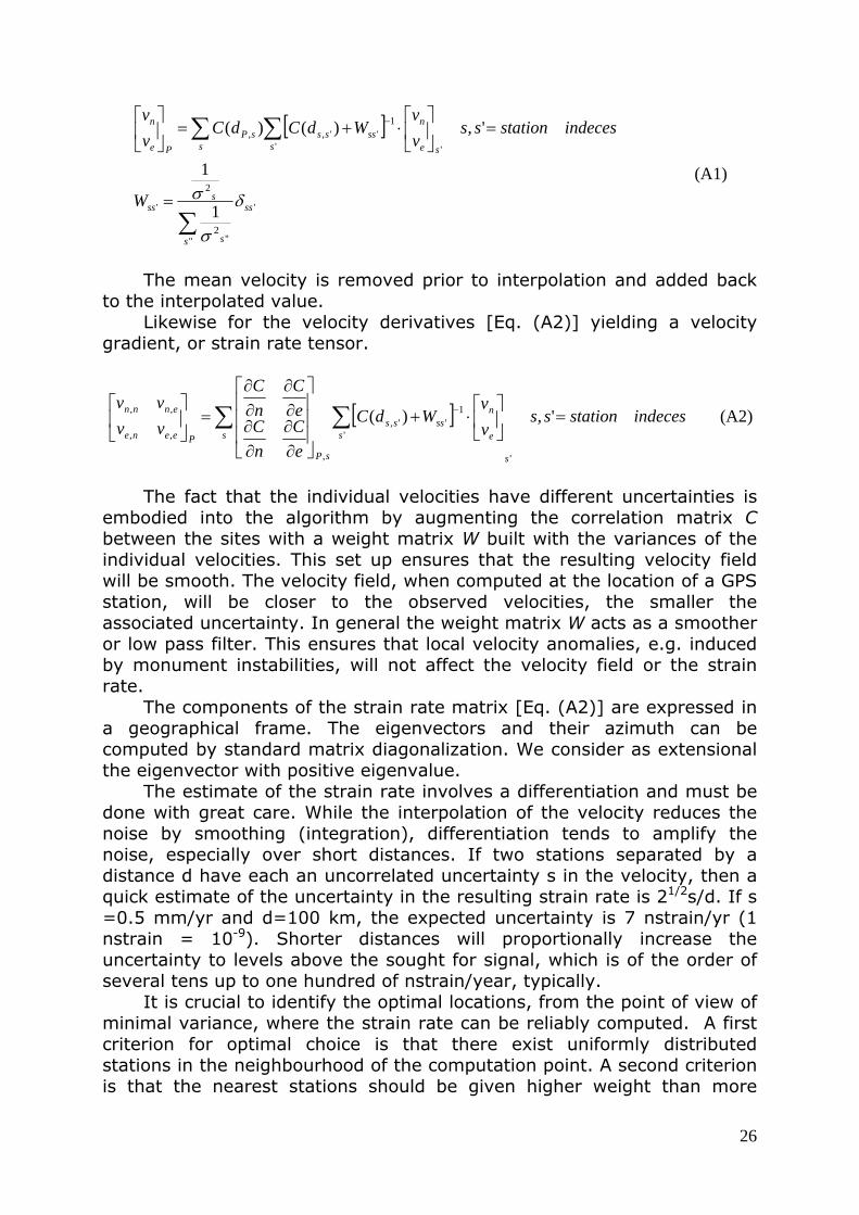
Once the velocities and their uncertainties are given at each GPS station, and the correlation function has been specified, the velocities and their uncertainties can be interpolated at other points P by a minimum variance (or ‘optimal’) algorithm known as least squares collocation:

26

[ ]

'

'' ''2

2

'

''

1'',,

1

1

',)()(

ss

s s

sss

ss s e

nsssssP

Pe

n

W

indecesstationssvv

WdCdCvv

δ

σ

σ

∑

∑ ∑

=

=⎥⎦

⎤⎢⎣

⎡⋅+=⎥

⎦

⎤⎢⎣

⎡ −

(A1)

The mean velocity is removed prior to interpolation and added back

to the interpolated value. Likewise for the velocity derivatives [Eq. (A2)] yielding a velocity

gradient, or strain rate tensor.

[ ] indecesstationssvv

WdC

eC

nC

eC

nC

vvvv

s

s s e

nssss

sP

Peene

ennn =⎥⎦

⎤⎢⎣

⎡⋅+

⎥⎥⎥

⎦

⎤

⎢⎢⎢

⎣

⎡

∂∂

∂∂

∂∂

∂∂

=⎥⎦

⎤⎢⎣

⎡∑ ∑ − ',)(

'

'

1'',

,

,,

,, (A2)

The fact that the individual velocities have different uncertainties is

embodied into the algorithm by augmenting the correlation matrix C between the sites with a weight matrix W built with the variances of the individual velocities. This set up ensures that the resulting velocity field will be smooth. The velocity field, when computed at the location of a GPS station, will be closer to the observed velocities, the smaller the associated uncertainty. In general the weight matrix W acts as a smoother or low pass filter. This ensures that local velocity anomalies, e.g. induced by monument instabilities, will not affect the velocity field or the strain rate.

The components of the strain rate matrix [Eq. (A2)] are expressed in a geographical frame. The eigenvectors and their azimuth can be computed by standard matrix diagonalization. We consider as extensional the eigenvector with positive eigenvalue.

The estimate of the strain rate involves a differentiation and must be done with great care. While the interpolation of the velocity reduces the noise by smoothing (integration), differentiation tends to amplify the noise, especially over short distances. If two stations separated by a distance d have each an uncorrelated uncertainty s in the velocity, then a quick estimate of the uncertainty in the resulting strain rate is 21/2s/d. If s =0.5 mm/yr and d=100 km, the expected uncertainty is 7 nstrain/yr (1 nstrain = 10-9). Shorter distances will proportionally increase the uncertainty to levels above the sought for signal, which is of the order of several tens up to one hundred of nstrain/year, typically.

It is crucial to identify the optimal locations, from the point of view of minimal variance, where the strain rate can be reliably computed. A first criterion for optimal choice is that there exist uniformly distributed stations in the neighbourhood of the computation point. A second criterion is that the nearest stations should be given higher weight than more

27

distant stations, if their velocities have the same variance. This last criterion is automatically satisfied by the collocation algorithm. To ensure that the strain rate is computed at points such that it is sufficiently well constrained by data from neighbouring stations we have adopted the following rule: the strain rate is computed at the geographical location of those permanent stations of known velocity, such that at least one additional station with known velocity exists in each quadrant within a radius equal to the correlation distance d0.

The adopted rule is exemplified in Figure A3. We require that within a circle of radius d0 five velocities are defined: the velocity at the center of the circle and at four additional sites. The least squares collocation represents in a continuous form a finite difference between the center velocity and the peripheral velocities. In this manner we ensure that the resulting strain rate reliably describes the rate of deformation in the circled area. Unfortunately the strain rate computed by this rather conservative approach not always relates to areas of seismological interest. Mapping the strain rate to other locations is mathematically feasible but not recommended, due to the fast increase of the variance.

A3. Numerical results The numerical results for northern, central and southern Italy

obtained with the velocities of permanent GPS stations resulting from the combined analysis described above were used as geodetic constraints in the computation of the earthquake occurrence probabilities (Table 2). For southern Italy we have a number of stations insufficient to meet the adopted criterion for strain rate computation. Therefore we have used a set of velocities coming from campaign and permanent stations, available from the literature and processed by Analysis Centers outside the EUREF network. For this reason we have thought it appropriate not mixing the sets of velocities, although the methodologies of computation are, in a broad sense, consistent with each other.

APPENDIX B: Finite-element modelling The finite-element modelling aimed to reproduce a large amount of

neotectonic data for Italy by means of trial-and-error approach, using thin-shell finite element code SHELLS (Bird, 1999), in a large number of iterations which mostly differ by boundary conditions, fault friction coefficient (as for example in Barba, 2007; Barba et al., 2008; 2009). In all these studies, model predictions were compared to three independent datasets: geodetic horizontal velocities from temporary and permanent GPS stations (Serpelloni et al., 2007; Caporali, 2007); stress regime data, based on relative stress magnitudes, and; the directions of maximum horizontal compressive stress (Montone et al., 2004). Residuals between model predictions and the calibration datasets allowed to characterize of

28

the degree of realism of the numerical results. The model results that exhibited the lowest misfits were averaged, thereby accounting for uncertainties in boundary conditions and model parameters. Misfits were standardized to account for the different calibration datasets.

The model incorporates faults and realistic rheology in a two-layer grid (crust and lithospheric mantle) with laterally-varying seismogenic thickness, heat flow and topography. The horizontal components of the momentum equation (Kong and Bird, 1995) were solved to predict long-term horizontal velocities, anelastic strain rates, vertically integrated stresses, and fault slip rates.

In the thin-shell neotectonic modelling program SHELLS (Bird, 1999, and references therein) uses isostasy and vertical integration of lithospheric strength to reduce the three-dimensional problem of deforming lithosphere to two dimensions, where the horizontal velocity components do not depend on the depth. The components of the momentum equation are vertically integrated using 1-km-steps at each of seven Gauss integration points in each finite element (continuum or fault) and the horizontal components of velocity predicted. The vertical component of the momentum equation comes from the assumption of isostatic equilibrium (Bird, 1989). The model is composed by 2 layers with variable thickness, plus topography. Temperature, strength and the shear stress tensor are depth dependent. By integrating the shear stress along z the problem is reduced to plane strain. Computing the corresponding strain solution using only the in-plane terms makes problem bidimensional. SHELLS solves the momentum equation in two dimensions,, and the vertical normal stress - assumed as lithostatic - is then added to the result.

The rheology has the same analytical form at all points of the model. The code neglects all elastic strain accumulation and release and solves for velocities, fault slip rates, and anelastic strain rates and stresses. Deformation occurs by frictional sliding or nonlinear dislocation creep. Given a strain rate, the deviatoric stress is evaluated separately for each of three flow laws: frictional faulting, dislocation creep (power law), and Newtonian creep (linear). At each point, the flow law that provides the lowest maximum shear stress is selected. The rheological parameters are different for the crust and mantle lithosphere. The rheological parameters impose the lithospheric rigidity and the coupling between the crust and the lithospheric mantle. The chosen parameters represent an average lithosphere. Frictional faulting stress is evaluated under the assumption of hydrostatic pore pressure. Faults are distinguished from continuum elements because of double “slipping” nodes, and a lower frictional coefficient with respect to the continuum medium.

The method incorporates some 3-D characteristics since volume integrals of density and strength are performed numerically in a lithosphere model with laterally varying crust and mantle-lithosphere layer thicknesses, heat flow, and elevation. Crustal and lithospheric mantle structure, and steady state thermal regime have been derived from literature data.

sausage 22/7/09 14:27 1

Fig. 1 - Seismogenic areas (red) and mapped faults (yellow) in the Italian Seismogenic

Source Database.

sausage 22/7/09 14:27 2

Fig. 2 – M0R (in N⋅m/yr) computed from GPS observations. Blue small dots for M0<1.0⋅1018; red medium dots 1.0⋅1018≤M0<2.0⋅1018; purple medium circles 2.0⋅1018≤M0<3.0⋅1018; black large circles M0≥3.0⋅1018. The central GPS station of each domain is marked by a square with size and colour according to its M0. The numbered large circles identify the four domains: 1 = eastern Alps, 2 = western Alps, 3 = central Apennines, 4 = southern Apennines.

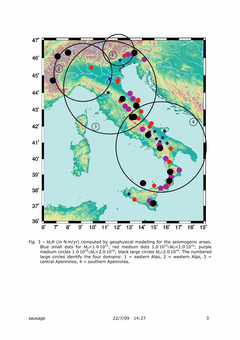
sausage 22/7/09 14:27 3

Fig. 3 – M0R (in N⋅m/yr) computed by geophysical modelling for the seismogenic areas. Blue small dots for M0<1.0⋅1015; red medium dots 1.0⋅1015≤M0<1.0⋅1016; purple medium circles 1.0⋅1016≤M0<2.0⋅1016; black large circles M0≥2.0⋅1016. The numbered large circles identify the four domains: 1 = eastern Alps, 2 = western Alps, 3 = central Apennines, 4 = southern Apennines.

sausage 22/7/09 14:27 4

Fig. 4 – M0 release since 1700 in the 4 domains: a) eastern Alps; b) western Alps; c)

northern Apennines; d) southern Apennines. Solid line for all earthquakes of the Italian earthquake catalogue (Gruppo di lavoro CPTI, 2004), dashed line for events with an MW 5.5 and over. The vertical scale varies in the different panels.

Figure 5. Mapped and modelled faults in the eastern Alps domain: a) seismogenic areas

(pale grey areas marked by ITSA) and mapped faults (dark grey areas marked by ITGG); b) magnitude distribution (black columns for the mapped faults and grey columns for the modelled faults).

sausage 22/7/09 14:27 5

Figure 6. 30-year probability for Mw≥6.0 and over according to a Poisson model: a)

computed by geodetic constraints; b) computed by geophysical constraints. Blue small dots for P≤1%; red medium dots 1%<P≤2.5%; purple medium circles2.5%<P≤5%, black large circles P>5%.

Figure 7. 30-year probability for Mw≥6.5 and over according to a Poisson model: a) computed by geodetic constraints; b) computed by geophysical constraints. Blue small dots for P≤0.4%; red medium dots 0.4%<P≤1.5%; purple medium circles 1.5%<P≤3%, black large circles P>3%.

sausage 22/7/09 14:27 6

Fig. 8 – Comparison of the probability estimates (P1 indicate the exceedance probability

in 30 years computed with geodetic constraints, P2 indicate the exceedance probability in 30 years computed with geophysical constraints): a) P2 vs. P1 for magnitude 6.0; b) P2 vs. P1 for magnitude 6.5; c) P1 for magnitude 6.5 vs. P1 for magnitude 6.0; d) P2 for magnitude 6.5 vs. P2 for magnitude 6.0.

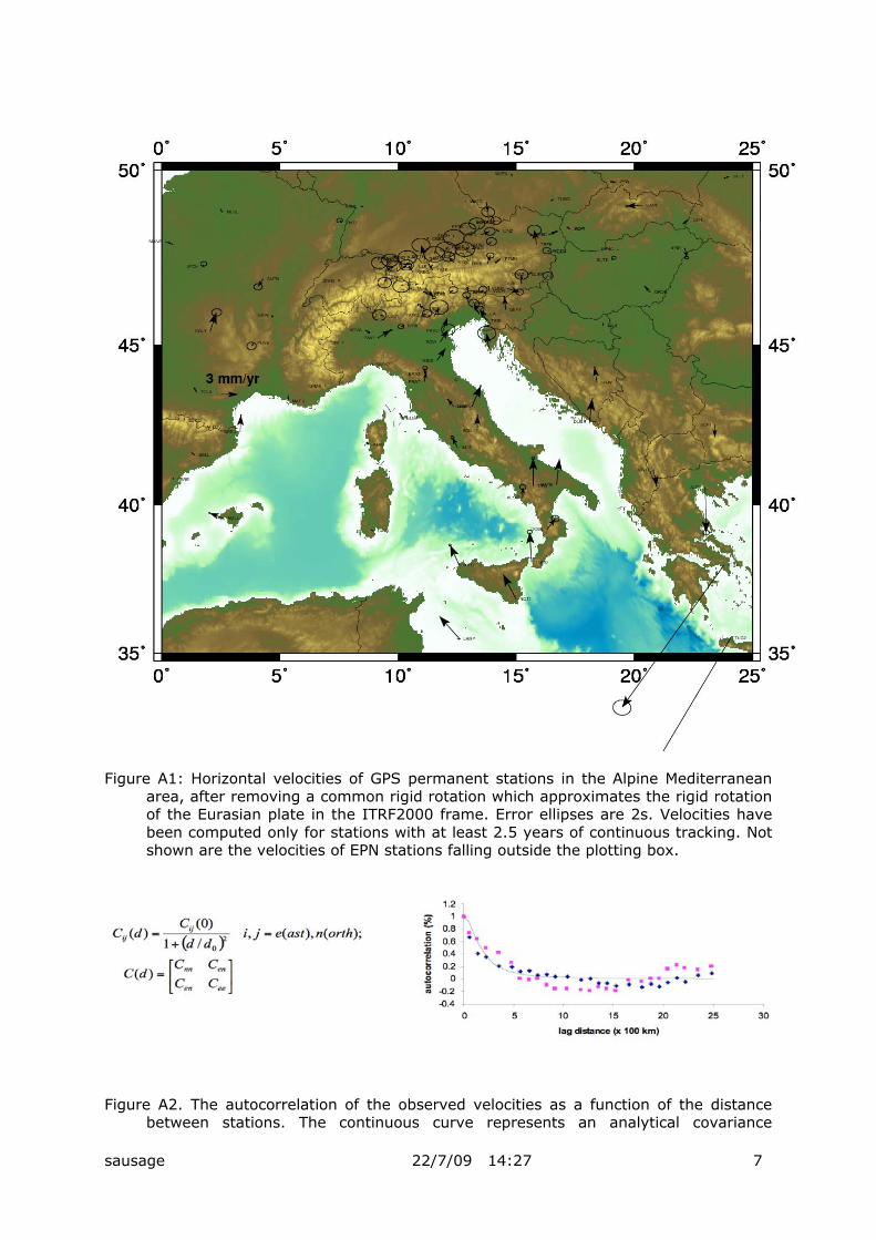
sausage 22/7/09 14:27 7

Figure A1: Horizontal velocities of GPS permanent stations in the Alpine Mediterranean

area, after removing a common rigid rotation which approximates the rigid rotation of the Eurasian plate in the ITRF2000 frame. Error ellipses are 2s. Velocities have been computed only for stations with at least 2.5 years of continuous tracking. Not shown are the velocities of EPN stations falling outside the plotting box.

Figure A2. The autocorrelation of the observed velocities as a function of the distance

between stations. The continuous curve represents an analytical covariance

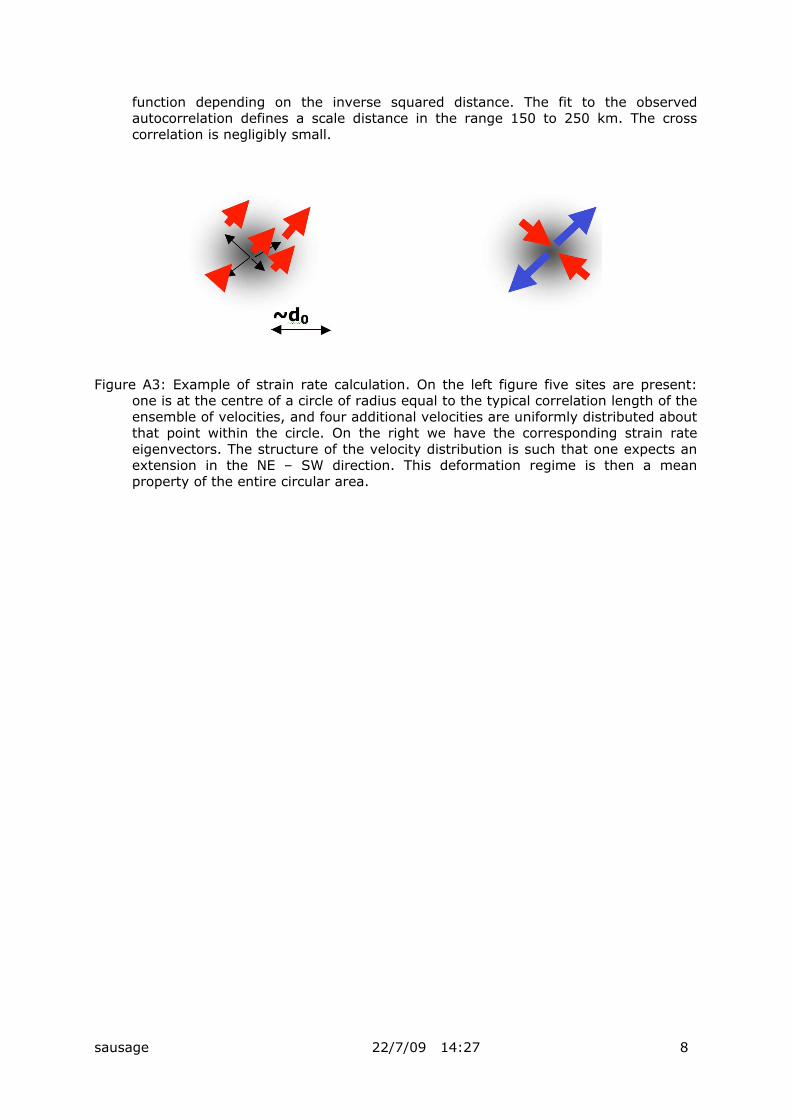
sausage 22/7/09 14:27 8

function depending on the inverse squared distance. The fit to the observed autocorrelation defines a scale distance in the range 150 to 250 km. The cross correlation is negligibly small.

Figure A3: Example of strain rate calculation. On the left figure five sites are present:

one is at the centre of a circle of radius equal to the typical correlation length of the ensemble of velocities, and four additional velocities are uniformly distributed about that point within the circle. On the right we have the corresponding strain rate eigenvectors. The structure of the velocity distribution is such that one expects an extension in the NE – SW direction. This deformation regime is then a mean property of the entire circular area.