Occurrence of Transients in Water Distribution Networks

Procedia Engineering 119 ( 2015 ) 1473 – 1482

Available online at www.sciencedirect.com

1877-7058 © 2015 Published by Elsevier Ltd. This is an open access article under the CC BY-NC-ND license (http://creativecommons.org/licenses/by-nc-nd/4.0/).Peer-review under responsibility of the Scientific Committee of CCWI 2015doi: 10.1016/j.proeng.2016.01.001

ScienceDirect

13th Computer Control for Water Industry Conference, CCWI 2015

Occurrence of transients in water distribution networks

Dagmara Starczewskaa*, Richard Collinsa and Joby Boxalla aPennie Water Group, Department of Civil and Structural Engineering, University of Sheffield, Sheffield, S1 3JD, UK

Abstract

The common existence of pressure transients in operational water distribution systems (WDS) requires their characterisation and assessment of their impact. This paper performs such characterisation by evidencing the occurrence and the differences in pressure transient behaviour in complex WDS. Ten samples of continuously recorded high resolution pressures from diverse networks and sources were analysed. The presented pressure traces show regular and occasional pressure transient waves in various complex networks. Histogram analysis of the rate of change of head provides some insight into transient behaviour in these sites. Although there was no distinct correlation between network characteristics (ie. length, diameter, age) and transient behaviour, network complexity was observed to change the transient characteristics. Transient characteristics were observed to be strongly influenced by likely sources, in particular commercial customers. The data highlights the need to understand, quantify and characterise transients and hence link to possible impacts, such as structural or water quality failures. © 2015 The Authors. Published by Elsevier Ltd. Peer-review under responsibility of the Scientific Committee of CCWI 2015.

Keywords: water distribution system; transients; characterisation

1. Introduction

Water distribution systems (WDS) are complex networks whose main function is to maintain a reliable safe supply of water. Current regulation of WDS in the UK requires monitoring of pressure in networks, usually undertaken at 15 minutes intervals. This resolution is not fast enough to capture changes in pressure due to the water hammer (pressure transient) effect; therefore the current knowledge of the existence of these fast events in operational networks is largely unknown.

Some studies highlighted the fact that the presence of pressure transient waves are actually seen in operational and complex WDS [1–3], therefore these systems should no longer be considered as static or pseudo-static. This paper adds further evidence to support this statement and presents one possible way to analyse such changes. It provides information about the pressure transient occurrences, nature and the importance of the possible sources of transients in operational WDS.

* Corresponding author. Tel.: +44 114 222 5732; fax: +44 114 222 5700.

E-mail address: [email protected]

© 2015 Published by Elsevier Ltd. This is an open access article under the CC BY-NC-ND license (http://creativecommons.org/licenses/by-nc-nd/4.0/).Peer-review under responsibility of the Scientific Committee of CCWI 2015

http://crossmark.crossref.org/dialog/?doi=10.1016/j.proeng.2016.01.001&domain=pdf

http://crossmark.crossref.org/dialog/?doi=10.1016/j.proeng.2016.01.001&domain=pdf

1474 Dagmara Starczewska et al. / Procedia Engineering 119 ( 2015 ) 1473 – 1482

2. Background

The importance of understanding transient behaviour is due to the damage that transients may be causing to our vital WDS. There are two possible categories of damage from pressure transient events. The first has been largely documented in the literature as a catastrophic failure due to high magnitude force caused by fast pressure transient waves. These events were usually seen in large pumping mains and caused damage to the water network or equipment [4, 5]. In these scenarios the casual link between the failure and the transient is easy to determine. The second is the fatigue-like failures due to prolonged impact of smaller magnitude transients over a long time. This cause of fatigue has been recognized [6] but it has not been possible to fully explore. This is primarily due to the large time scales involved, failures may require many thousands of transients, and lack of long term high quality transient data. There is also a potential for transients contributing to water quality failures [7–9].

Real WDS systems tend to be large, complex and exhibit a large amount of uncertainty. Therefore current understanding of pressure transient behaviour is limited to simple networks. It is known that pressure transient magnitudes vary with factors such as a path, a length of the conveyance pipeline, diameter, thickness and type of a pipe (viscoelastic effect) [10, 11]. There is also a perception that network complexity should dissipate transients, while some modelling work [12, 13] suggests the opposite. Due to the lack of available high resolution transient data it is, to date, difficoult to categorically confirm or refute the results of the modelling studies and generalize to more networks.

There are a number of studies that consider the potential sources of transients. A comprehensive list of such can be found in the literature [14, 15]. Transient waves can be caused by any operation (planned, routine or accidental) which rapidly changes steady-state conditions of fluid flow in a pipe. It is known that a rapid closure of a valve and malfunction of other network instrumentation can cause pressure transients, therefore a number of occasions and possible sources of transient exists in operational WDS. Pump operating (switching on and off) is one of the commonly recognised and the most frequently analysed transient source [16–18]. Industrial activity can also produce large numbers of transients due to water being drawn at a fast rate from the network. The relative importance of such impacts and their likeness to occur in live WDS, have not been sufficiently documented and characterised yet.

The aim of this study was to explore the occurrence of pressure transients in several operational WDS and any site specific characteristic that may correlate with network properties and possible dissipation effects. This paper will also explore methods to better present and quantify the transient response of a WDS.

3. Method

In the UK the WDS are subdivided into District Metered Areas (DMAs). The WDS investigated in this paper include five typical UK DMAs. Sites were chosen to represent the complexity of the water network with looped and branched connections included, see Figure 1. Two of these sites were gravity fed (Figure 1 Site 1 and 5) and the remaining three were supplied by a pumping station (Figure 1 Site 2, 3 and 4). Only one site was directly supplied by a pump (Site 2, Figure 1). Site 3 was supplied by a pump, which was about 5.72 km away from this site. This connection, however, was not direct and proceeded by series interconnected DMAs. The situation was the same in Site 4 with the pump in the distance about 5.66 km from the site.

Figure 1. Network configuration for monitored sites, site boundaries in bold. (1) Site 1, (2) Site 2, (3) Site 3, (4) Site 4, (5) Site 5. Two monitored points per each site are marked as a) and b). Rectangles mark the inlets to the DMAs.


monitoring for this period of time. Loggers were deployed on standard and easily accessible fire hydrants and system washouts. The pressure data was collected using 100Hz resolution which allowed the capture of pressure transient waves in operational WDS.

3.3. Noise

In the pressure data obtained from WDS the unpredictable noise variations in the signal are observed over entire recording period. The presence of which has an impact on the quality of the data. Therefore to improve it a noise reduction was undertaken.

Power spectral density (PSD) was used to check a frequency response of the signals and to determine a cut off frequency. Different ranges of cut off frequencies were checked and the frequency of 7Hz was decided to be used. This frequency allowed for a signal to retain a part of ‘flat’ power, which means that sufficient/important information in the signal was left and part of the instrument noise was removed. Prior to the analysis pressure data were filtered using a finite impulse response (FIR) filter to remove instrument noise with a cutoff frequency 7Hz, and 5Hz transition width.

3.4. Assessment method

Visual assessment of the whole 13 day long pressure traces does not show the fine detail of the pressure waves. This information can be revealed by repeatedly zooming into various sections of the trace. That could be done for an initial assessment but it would remain highly subjective and be very time consuming. Visual assessment can also be misleading as the transient events can be masked by the diurnal pressure patterns, which would need to be removed to show real transient events.

Production of a histogram of the pressure data can help to illuminate, and quantify, the pressure response of the system. However it was found that although providing more easily comparable data between sites the impact of the diurnal patterns was still masking the some of the transient responses. The representation of the data as plots of rate of change of head with respect to time ( h/ t) was then chosen as better assessment method. This method reveals how fast the pressure transients events are happening. Histograms of rate of change of head with respect to time ( h/ t) were then undertaken to aid a visual assessment of the pressure traces. Due to the large number of small scale fluctuations in the pressure traces, dominating over the larger events, a logarithmic scale is used for the y-axis of the histograms to ensure that all events are visible.

4. Results

For the clarity of this paper the results from five sites were pre-ordered by magnitudes of transient events seen in the pressure traces. These were ranked from highest to lowest. This ranking was also followed in the ordering of the sites already presented in Figure 1, Figure 2 and Table 1.

4.1. Time series data

Figure 3 shows time series data from ten locations in five sites, two points for each site. From this figure it can be seen that Site 1 experienced regular intervals of transient activities. Figure 3 1a) and 1b) show that this site had regular transient activities observed typically from 7:00 am until 10:00 pm with a frequency of up to 11 times per hour and then decreased significantly from 10:00 pm to 7:00 am. The sudden decrease in pressure transient activity seen in the pressure trance happened on 26 December (national holiday). Transient activities did not decrease at weekends. The average magnitudes of these events were about 10-25 head (m) at location a) and 5-10 at location b). In this site the static pressure were different for two locations because of the difference in elevation between points.

Site 2 showed regular pressure transient activities occurring continuously through an entire monitoring period, sometimes up to 20 times during the day. Pressure traces from this site showed different steady state heads and different size of transients. Average magnitude of pressure transients were about 12 head (m) for upsurge and 10 head (m) for downsurge pressure transient events at location a). Pressure trace from the location a) showed that source of the transient was close to this location. The pressure trace from the location b) had the same transients and additional diurnal steady state patterns characteristic for domestic consumption. The transients are clearly still seen but their magnitudes decreased to about 8 head (m) for upsurge and 6 head (m) for downsurge.

Pressure traces from Site 3 showed a regular transient pattern of series upsurge and downsurge events about 5 - 10 head (m) in magnitudes at location a) and around 10 head (m) at location b). It was seen that these traces occurred on average 30 times per day, usually between 6:00 am and 6:00 pm. Figure 3 3a) and 3b) shows a clear pattern of regular transients seen on weekdays but not on weekends. Location a) in this site was close to the inlet of the DMA. The other location was further away from the inlet and lower in elevation by about 10 m.

Sites 4 and 5 showed evidence of infrequent and occasionally occurring transients (typically one significant transient event of a magnitude above 8 head (m) in Site 4 and 10-15 head (m) at Site 5 per week). In both sites diurnal pressure responses and daily patterns of domestic consumption dominated the pressure traces. There was no much difference in steady state pressures between points a) and b) in the sites, both locations were at approximately the same elevation.


4.2. Histograms of head change rates with respect to time

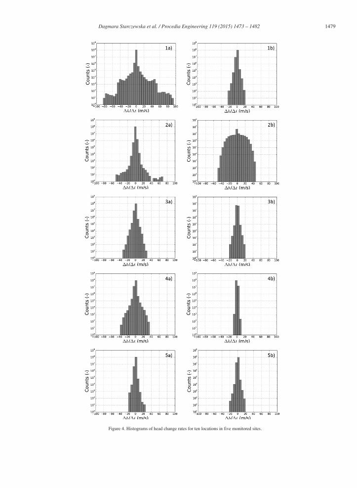
Figure 4 presents histograms of rate of change of heads in the logarithmic scale for all ten pressure traces in five sites, two locations per each site. Because most of the data for all histograms was centered around zero with standard deviation from 0.67 (Site 4, location b)) to 11.3 (Site 2, location b)), the logarithmic scale was used to show variability occurring in tails of the histograms at each location.

It can be seen that Site 1 (location a) showed the most variability in changes of pressure head in comparison to the rest of the sites. The spread of the histogram covered a range of values from about -80 to 95 (m/s), and the shape of the histogram was approximately symmetric around its median. A non-homogenity in the shape of the histogram was noticed. It was seen as three different regimes/behaviours. First one occurred in ranges from -80 to -50 and from 50 to 95 (m/s), the second one from -50 to -25 and from 30 to 50 (m/s) and the third one from -25 to 30 (m/s). Location b) showed much less variability in changes of head and spread of the data was reduced to range from about -23 to 20 (m/s).

Site 2 was the second in terms of the variability of the h/ t values. These ranged from about -50 to 70 (m/s) at location a) and from about -50 to 47 (m/s) at location b). Location a) showed some outliers in the range from 45 to about 70 (m/s). Histogram at location b) had characteristic shape which was due to the fast changes in h/ t recorded at this location. Changes in pressure head happened in a different (faster) time scale in comparison to the data gathered from location a). Histogram from this location showed that pressure data was much more dynamic and fast than at any other locations.

Histograms for both locations in Site 3 had roughly triangular shape. The spread of the data was from -32 to 30 (m/s) at location a) and a bit less (from -20 to 20 (m/s)) at location b). The shape of the histogram at location a) was approximately symmetric.

The histogram for location a) in Site 4 was very similar to the location a) in Site 3. Both histograms had symmetric shapes. Location b), however, showed very uniform variability in changes of head (from -38 to 36 (m/s)). The data at location b) covered the least ranges of values in comparison to any other sites (from -9.5 to 11 (m/s)). This shows that there was less variability in head changes at this location.

Histograms in Site 5 had very similar ranges; however the histogram at location a) was slightly skewed to the right. The data ranges were from -17 to 25.5 (m/s). The histogram at location b) showed some similarities in shape to the histogram in Site 3, location b) with ranges from -21 to 20 (m/s).


Figure 3. Pressure data for 13 days from two locations within the selected sites. (1) Site 1, (2) Site 2, (3) Site 3, (4) Site 4, (5) Site 5. On the left hand side pressure traces from the locations a), on the right site locations from the locations b) for each site respectively (see Figure 1 for the locations of the points in

networks). Point zero on the x axis represents midnight in different week days.


Figure 4. Histograms of head change rates for ten locations in five monitored sites.


5. Discussion

5.1. Interpretation of pressure data

Visual assessment of pressure traces does not allow for quantitative analysis of pressure waves seen in the pressure trace. The eye is dominated by what is perceived to be a regular occurrence. For instance based on the visual assessment Site 1 shows one possible characteristic transient type which is happening there ± 30 head (m) at location a) or ± 5-10 head (m) at location b). Based on location a) Site 2 would have two or even three transient types. The first would be about 10 head (m), the second about 20 head (m) and third one above 20 head (m), occurring occasionally. This type of assessment does not show what is really happening in these sites. Only a detailed assessment can reveal that Site 2 had only two types of transients; an upsurge and downsurge as highlighted in the result section. Due to the upsurge the overall pressure goes up, stays there and then goes down due to the downsurge and remains there until a further upsurge. Furthermore, relying only on visual comparison between sites it can be seen that Site 2 looks like it has the highest amounts of transients, much more than Site 1 or any others. Only by looking at the head change rates in the histogram can it be seen that actually Site 1 has lots of different magnitudes of transients and this site has the highest variability in changes in pressure heads, see Figure 4. The steady state pressure in the middle of the histogram is very constant, which can be confirmed by its pressure trace.

Location b) in Site 2 showed very fast changes in pressure head captured in the characteristic shape of its histogram. That behaviour was not observed in location a) or in any other sites, based on theirs histograms. This behaviour was not able to be noticed in its pressure traces.

Pressure traces form Site 3 at locations a) and b) were roughly similar. There were slight differences in pressure transients magnitudes and static pressures as described in the Results section. The histograms from both locations were roughly similar, but more variability in changes in pressure head was seen at location a).

Pressure traces from Site 4 at locations a) and b) were very similar in that there were transients ± 5 head (m) of magnitude happening over entire recording period. However the histograms from the location a) and b) proved that these points had different pressure responses. Location a) had more variability in changes of pressure head then location b) as described in the Results section.

In contrast to Site 4, Site 5 had very similar pressure traces at both locations. The similarities were also seen in the histograms (see the Results section).

Furthermore the histograms of head change rates for locations a) and b) in Site 1 showed that pressure responses are different at these two points. That was possibly due to the fact that the measuring point was either close to the inlet to the DMA or to the source of transient. Therefore different pressure transient responses are seen in the sites which corresponded to different types of transient due to its source and location in the network. This shows that in some cases it may be important where the pressure traces were captured in the network. For these sites one monitoring point may not be enough to completely characterise the DMA pressure response. In other cases, there were sites where pressures were very similar, so location of the measuring point may not matter. In Site 3, histograms of head change rates were very similar for locations a) and b). This may indicate that the location of the measuring point in the network did not matter for this particular site.

Some locations have shown that only their histograms of head change rates can reveal more information about transient pressure response. Although the histograms reveal more information about pressure changes than visual assessment these are limited and not able to fully capture all behaviour of pressure transients. This is due to the fact that the t is a fixed function and does not actually define pressure transient events and does not allow the capture of time durations and the number of occurrences of pressure transient waves. For instance in Site 4 changes in pressure head are happening faster whereas changes in pressure head are slower, but higher in magnitudes in Site 5.

5.2. Correlation of transient behaviour with network characteristics

In this section the network characteristics (described previously in Table 1) that may affect/influence the pressure wave were investigated. By looking at network characteristics it was noticed that pressure transient ranks may possibly correlate with pipe materials, lengths, diameters or age, however due to their strong regular patterns it could also be related to the number of commercial properties seen in the area. Commercial users, by rapidly drawing water from the network, could indeed cause pressure transient events.

From literature, pipe material is expected to have one of the most significant impacts on the pressure transient behaviour of a system. The rigid linear elastic nature of metals and asbestos cement allows a greater change in pressure for a given change in fluid velocity. It is known that the visco-elastic behaviour of plastic pipes influences pressure transient wave by attenuating the pressure fluctuations and by increasing the dispersion of the travelling wave [19]. From Table 1 it can be seen that the percentage of metal pipes in the network does not provide a good description of the ranking of the magnitudes of the transients at the 5 sites (1-5). Sites 4 and 5 have the most metal pipes and the lowest transient response, whilst Sites 1 and 2 have similar amounts of metal and a much higher transient response. Site 3 has the lowest metal percentage and again a significant transients response. A much better explanatory factor for the raking can be found by looking at the percentage of plastic pipes in networks. Sites 1, 2 and 3 have lower percentages of plastic (5.8 – 7.6%) and high transient activity, whilst Sites 4 and 5 have much higher


percentages (12 an 15.3% respectively) and a much lower transient response. Whilst the percentage of plastic pipes correlates with the magnitude of the transient response, it does not appear to be able to describe the differences in the shapes of the traces seen.

The wave speed in a pipe, and consequently the potential change in pressure due to a change in velocity are affected by the diameter of a pipe (and the wall thickness). In addition the magnitude of pressure transient waves increase when travelling through a sudden contraction and decrease due to sudden expansion [20]. Therefore the distribution of diameters in the DMA could help to explain the ranking of the transient response. It can be seen from Figure 2b that the range of pipe diameters and their relative percentages in each of the investigated sites was very similar; therefore this characteristic was not able to explain differences in pressure transient behaviours.

Age is a surrogate for many different processes that might effect the propagation of transients in a network. Typically older pipes experience greater leakage (a large transient dissipation mechanism [21, 22]), are more subject to corrosion (weakening the pipe and reducing the wave speed [23, 24]). Site 1 had the oldest network (40% of the network was comprised of 165 years old pipes), whereas Site 3 was quite young (85% of 65 years old pipes), both these sites showed significant transient response. Sites 4 and 5 showed limited transient activities. Site 5 was the youngest amongst the sites and Site 4 was also a young site. Therefore the relation between pipe age and the presence of pressure transients was also not observed.

Each time the wave passes through a junction a proportion of the wave is reflected with the rest propagating further into the system. That could cause dissipation or amplification of the pressure transient wave. The measure of complexity of the network utilized in this paper did not showed that that could have an effect on the pressure traces. Site 1 has the highest complexity as it average pipe length was the smallest. Rest of the sites had roughly the same rank of the network complexity. That therefore could not be used as sufficient explanation for the different behaviour of pressure trances seen in the sites.

As large users of the water, commercial properties have the potential to produce significant transient events. It is therefore hypothesised that the transient activity in a site may correlate with the percentage of commercial users. However this was not seen. Site 1 had over 50% commercial properties and a large transient response, however all the other sites had less than 3.5% commercial properties (and very similar values) and a very varied transient response. Therefore it can be seen that the simple metric of percentage of commercial properties is not useful, however further investigation of the traces implies that commercial users may be a significant cause of the transient response seen.

From this analysis it can be seen that of the network metrics available only the percentage of plastic pipe was able to describe the ranking of the sites due to the magnitudes of their transient responses. However, it does not appear to be able to describe the differences in the shapes of the traces seen.

5.3. Correlation of transient behaviour with potential source of transient

As described in the Result section in some sites pressure traces stop during the weekend (Site 3) or during the night hours (Site 1). That could suggest a possible commercial user as a source. Site 1 showed a regular pressure transient pattern which did not decrease at weekends, however the sudden decrease in pressure transient activity on a national holiday could also confirm a possible industrial source of these pressure transients.

Site 3 had very few commercial properties of only about 2%, but clearly weekday/weekend patterns were visible. It could be surmised that such regular pressure traces can be generated by a small number or possible only one commercial user. A commercial user was located possibly in the south of the site. This could be confirmed by pressure trances from both locations, where it can be seen that magnitude of pressure transients was higher at location a) than location b). Site 2 had a pump which directly feeds the entire site, as was previously described in the Method section. This site showed regular transient activities unrelated to week days or weekends, which on further investigation correlated with the pump switch on/off times.

Sites 4 and 5 were highly domestic with low percentages of commercial properties and no identified transient sources. Whilst it is not seen that the numbers of commercial properties has significance in explaining the existence of pressure

transient waves, rather it appears that the circumstances of the individual commercial properties may well do. For instance a brewery, a dairy or a swimming pool will have different impact on the water network than a shop or a hairdresser. In addition some businesses, by having badly controlled equipment, can have a more significant effect on the network than the others.

Different causes, primarily commercial users and pumps were found to cause the majority of the pressure transient waves in the investigated sites. This strongly suggests that the type of source of pressure transient and the closeness of the source to a section of network being investigated is a more important explanatory characteristic than the combination of the material, diameter, age and complexity of the network.

5.4. Possible impact of pressure transients

Extreme pressure transients have been understood to cause problems in simple systems comprised mainly of a single pipeline, however in more complex arrangements, the presence of transients has not been fully documented; therefore, structural failures of pipes were rarely attributed to the presence of pressure transients. The sites reported in this paper were all highly dynamic, with three of the five showing strong repeated transients throughout the duration of the monitoring and across the spatial extent of the network. The regularly occurring pressure transients pose a question about structural safety of WDS. The continuous impact of


such pressure transients could be contributing to the degradation of pipe materials, pipeline accessories, pipe support and causing instrument failures. Pressure transients and their contribution to a structure, such as pipe failure through fatigue loading, and water quality, such as discolouration due to increased dynamics shear stress forces requires further study.

If were possible to characterise pressure transient waves in WDS the link to structural and water quality failures would be able to be further investigated. The use of histograms of rate of change of pressure, as shown here, allows some characterisation of the transient response, but has been shown to not be fully explanatory. Full characterisation of pressure transient events is therefore essential to widen the understanding of the existence, characteristics and possible impact of pressure transients in WDS.

6. Conclusions

This paper presents high temporal resolution pressure data and analysis from two weeks of monitoring of ten different locations in five DMAs, two locations in each area. Histogram analysis of the rate of change of pressure was undertaken to improve on simple visual inspection of the time series data, bringing out information on the different transient characteristics between the sites. The data shows variations in the transients measured in each network, irrespective of network material, diameters, length etc., but correlating with likely sources. As might be expected a network with a pumped source showed significant activity, but equal or even higher activity was shown in industrial DMAs, little or no transient activity was evident in gravity fed domestic DMAs. The transient characteristics at any given location were observed to be a complex function of both the source and network complexity, with the signals persisting throughout the networks, being changed but not necessarily dissipated by the complexity. Overall this work evidences the widespread occurrence of transients within complex water distribution networks, and highlights the need to better understand them and what transient characteristics are associated with possible structural and water quality impacts.

Acknowledgements

The authors would like to thank the Yorkshire Water Ltd for their support and permission to publish.

References

[1] D. Starczewska, R. P. Collins, and J. Boxall, Transient behavior in complex distribution network: a case study, Proc. 12th Int. Conf. Comput. Control Water Ind. CCWI., Perugia, 2013.

[2] J. Creasey and D. Garrow, Investigation of Instances of Low or Negative Pressures in UK Drinking Water Systems - Final Report, UK, 2011. [3] R. W. Gullick, M. W. LeChevalier, R. C. Svindland, and M. Friedman, Occurence of transient low and negative pressures in distribution systems, J.

Am. Water Work. Assoc., vol. 96, no. 11, 2004, pp. 52–66. [4] C. Jaeger, Water hammer effects in power conduits, Civ. Eng. Public Work. Rev., vol. 43, no. 23, 1948, pp. 74–76, 138–140, 192–194, 244–246. [5] R. E. Morris, Principal causes and remedies of water main breaks, J. Am. Water Work. Assoc., vol. 59, no. 7, 1967, pp. 782–798. [6] F. B. F. Rachid and H. S. C. Mattos, Modelling the damage induced by pressure transients in elasto-plastic pipes, Meccanica, vol. 33, 1998, pp. 139–

160. [7] S. M. Mustonen, S. Tissari, L. Huikko, M. Kolehmainen, M. J. Lehtola, and A. Hirvonen, Evaluating online data of water quality changes in a pilot

drinking water distribution system with multivariate data exploration methods., Water Res., vol. 42, no. 10–11, 2008, pp. 2421–30. [8] A. Aisopou, I. Stoianov, and N. Graham, Modelling Discolouration in WDS Caused by Hydraulic Transient Events, Water Distrib. Syst. Anal., 2010,

pp. 522–534. [9] G. Naser, B. W. Karney, and J. B. Boxall, Red water and discoloration in a WDS: a numerical simulation, 8th Annu. Water Distrib. Syst. Anal. Symp.

2006, 2006, pp. 152. [10] L. . Kinsler, A. R. Frey, A. . Coppens, and J. V. Sanders, Fundamental of Acoustics, 4th ed. New York, Chichester: John Wiley & Sons, INC, 2000. [11] B. Massey, Mechanics of Fluid. Taylor and Francis, 2006. [12] J. Ellis, Pressure transients in Water Engineering A Guide to Analysis and Interpretation of behaviour. Thomas Telford Limited, 2008. [13] B. W. Karney and D. McInnis, Transient analysis of water distribution systems, J. Am. Water Work. Assoc., vol. 82, no. 7, 1990, pp. 62–70. [14] G. J. Kirmeyer, M. Friedman, K. Martel, D. Howie, M. LeChevallier, M. Abbaszadegan, and M. Karim, Pathogen intrusion into the distribution

system, AWWA Research Foundation and the American Water Works Association., 2001. [15] D. Misiunas, J. P. Vítkovský, and G. Olsson, Pipeline burst detection and location using a continuous monitoring technique, Adv. Water Supply, 2003,

pp. 89–96. [16] S. Meniconi, B. Brunone, M. Ferrante, C. A. Carrettini, C. Chiesa, C. Capponi, and D. Segalini, The skeletonization of Milan WDS on transients due to

pumping switching off: Preliminary results, Procedia Eng., vol. 70, 2014, pp. 1131–1136. [17] D. McInnis and B. W. Karney, Transients in distribution networks: Field tests and demand models, J. Hydraul. Eng., vol. 121, no. 3, 1995, pp. 218–

231. [18] A. K. Soares, D. I. C. Covas, and H. M. Ramos, Damping Analysis of Hydraulic Transients in Pump-Rising Main Systems, J. Hydraul. Eng., vol. 139,

no. 2, 2013, pp. 233–243. [19] A. Bergant, A. S. Tijsseling, J. P. Vítkovský, D. I. C. Covas, A. R. Simpson, and M. F. Lambert, Parameters affecting water-hammer wave attenuation,

shape and timing—Part 1: Mathematical tools, J. Hydraul. Res., vol. 46, no. 3, 2008, pp. 373–381. [20] S. Meniconi, B. Brunone, M. Asce, M. Ferrante, and C. Massari, Potential of Transient Tests to Diagnose Real Supply Pipe Systems : What Can Be

Done with a Single Extemporary Test, J. Water Resour. Plan. Manag., vol. 137, no. 4, 2011, pp. 238–241. [21] W. Nixon, M. S. Ghidaoui, M. Asce, and A. A. Kolyshkin, Range of Validity of the Transient Damping Leakage, no. 9, 2006, pp. 944–957. [22] X. Wang, M. F. Lambert, A. R. Simpson, M. Asce, J. A. Liggett, and J. P. V tkovsky, Leak detection in pipelines using the damping of fluid transients,

J. Hydraul. Eng., vol. 128, no. 7, 2002, pp. 697–711. [23] M. L. Stephens, M. F. Lambert, A. M. Asce, A. R. Simpson, and M. Asce, Determining the internal wall condition of a water pipeline in the field using

an inverse transient, J. Hydraul. Eng., vol. 139, no. 3, 2013, pp. 310–324. [24] J. Gong, M. F. Lambert, M. Asce, A. R. Simpson, and A. C. Zecchin, Detection of localized deterioration distributed along single pipelines by

reconstructive MOC analysis, J. Hydraul. Eng., vol. 140, no. 2, 2014, pp. 190–198.

Occurrence of Transients in Water Distribution Networks

Documents

Transcript of Occurrence of Transients in Water Distribution Networks