Occupational Self-Selection and the Gender Wage Gap:

Evidence From Korea and United States

Soo Kyeong Hwang*

Solomon William Polachek**

January 2004

JEL Codes: J31, J71, O15, O53 Key Words: Gender, Wages, Korea, Occupational Segregation

* Korea Labor Institute (KLI)

** Department of Economics, State University of New York at Binghamton (Binghamton University)

*** Versions of this paper were presented at a Labor Problems Conference at Academia Sinica in Taiwan and a

Labor Economics Workshop at Cornell University. We received helpful comments from participants of both,

especially John Abowd, Francine Blau, Ronald Ehrenberg, Feng-Fuh Jiang, Larry Kahn, and Allen Kelly.

Polachek is particularly indebted to the Industrial Relations Section at Princeton University for providing support

during his sabbatical, when much of the research for this paper was done.

ABSTRACT

Men and women are sorted differently into jobs. Women comprise 46.5% of the US labor

force, but only 9.9% of engineering are women. In contrast nursing is 92.8% female. This

difference in occupational structure is called occupational segregation. Occupational

segregation poses a number of questions. For example, is occupational segregation responsible

for the gender wage gap? Do women entering these female dominated jobs receive low

enough wages to bring down the mean earnings of all women? Would these women receive

low wages even if they had entered male jobs?

This paper examines occupational segregation’s role in explaining the gender wage gap.

Specifically, it tests whether the number of women incumbents in a job is negatively related to

workers’ wages. Contrary to popular belief, our results indicate that the proportion of a job

that is female does not lead to lower wages. After using the McFadden logit model to adjust

for the probability a women enters a women’s job, we find women entering female jobs

receive positive rewards, while men entering male jobs similarly receive higher wages. Thus

women in women’s jobs do relatively better than women in men’s jobs, and men in men’s jobs

do relatively better than men in women’s jobs. This means that the population sorts into jobs

to maximize their wellbeing. The results are robust both in Korea and the US. The relatively

advantageous position of women in female jobs is found to be associated with gendered

comparative advantages in job specific skills. For this reason intervention in the job sorting

process might have adverse unintended effects. Rather than raise women’s wages, women’s

wages could go down. Similarly, rather than diminish men’s wages, men’s wages could go up.

1

I. Introduction

Many argue that women are less free than men are to choose their jobs. In this

framework, discriminating employers relegate women to inferior dead end jobs. This type job

assignment results in occupational segregation whereby women are disproportionately

represented in poor quality low paying jobs. Many cite occupational segregation as the main

reason for the gender wage gap. There are two issues involved. One is job assignment. The

other is wage. As such, occupational segregation means women tend towards lower paying

menial jobs, thus lowering their economic wellbeing.

The typical description of occupational segregation focuses on the crowding model.

Barbara Bergmann (1974) advocates this approach. Her argument states that the labor market

is segmented into two sectors - a primary sector of mostly male jobs, and a secondary sector of

predominantly low-quality female jobs. Discrimination against women in the primary sector

2

(men’s jobs),1 forces women to find jobs in the secondary sector, creating an excess secondary

sector labor supply. This excess-supply lowers secondary job wages, putting women at a

disadvantage.

Though compelling, there are other explanations for occupational segregation. Perhaps

the most plausible is the human capital approach. The human capital model argues that

individuals select occupations based on meshing their own interests and skills with particularly

amenable job attributes. This “matching” model claims that each occupation exhibits unique

characteristics. These characteristics include required working hours, physical versus mental

strengths, quantitative versus verbal skills, people skills, and more. Further, each skill

requirement pays a given market wage. Individuals choose their jobs to maximize earnings,

given their own unique skills.

This “supply-side” explanation focuses on rational choice, based on an individual

getting the most lifetime earnings or utility out of a career. An example is the computer nerd

that is probably far better off with a computer job rather than a job in public relations, where

he would not have the prerequisite people skills. Similarly, a women anticipating dropping out

of the labor market to bear and raise children would best pick a job with small penalties for the

intermittent labor force participation required when one takes time out of the labor force. By

the same token, jobs that have non-pecuniary advantages in the form of flexible work

schedules, but that compensate for these amenities with lower wages, might be advantageous

1 The firms in this sector highly value firm-specific experience and low labor turnover so that women’s access to

this sector can be restricted by employers who believe women have more discontinuous labor market experience

or less commitment to on-the-job training than men (Osterman, 1984). Other male employees in the primary

sector may collectively conspire to keep women competitors out of their jobs (England, 1989).

3

to women weighed down with raising a family. Polachek (1975, 1981) and Becker (1985) are

proponents of this latter human capital approach to occupational self-selection.

Typically job characteristics that offer flexibility offer low compensation. By the same

token, demanding difficult grueling jobs often pay a wage premium. These proficiency-based

wage differences are known as “compensating” wage differentials. Compensating wage

differentials force the market to recompense those undertaking jobs with undesirable, arduous

and demanding tasks. Highly female-concentrated occupations are often perceived as the jobs

having the lowest wages and worst labor conditions to which only the less productive workers

apply. 2 This approach therefore claims that the wage gap between women’s job and men’s job

is partly caused by unmeasured worker-specific ‘quality’ (Macpherson and Hirsch, 1995).3

In any case, family responsibilities can cause women’s and men’s jobs to encompasses

different skills. In addition, job differences are reinforced if women and men have different

skill endowments for other, perhaps biological or psychological, reasons. Good matching

would induce women to prefer the jobs they do best. But it is not clear the match yields greater

wages, though one would guess women’s comparative advantage would at least increase their

relative wages in this endeavor compared to men.

We adopt hedonic wage estimation techniques to link an individual’s job choice to

wage. Hedonic wage estimation measures how particular job characteristics affect wages. To

2 Over time, however, the role of gender composition as a signal of labor quality will be reduced because low-

paying female occupations would attract relatively lower-quality males and lose many high-quality female

workers.

3 It may be induced from past occupational discrimination or because of social and familial preferences. In any

case, quality sorting of workers on gender composition may occur as long as there are sufficient differences in

current wages and labor conditions across jobs.

4

employ the method, we disaggregate jobs by the proportion of women incumbents. As such,

we investigate hedonic wage functions for particular observable job characteristics. In this

framework, we investigate the relationship between gender composition and wages.

As it turns out, by utilizing notions of comparative advantage, we call to question current

thinking regarding an occupation’s gender composition. We find that individual and job

characteristics explain wage, rather than an occupation’s gender composition. Thus we refute

the claim that number of females reduce an occupation’s wage. This will be the main point of

our paper.

The rest of the paper is organized as follows. Section II presents the analytical

framework to examine a link between occupational sex segregation and wages. It argues that

jobs are defined by their unique characteristics. Workers choose jobs by matching their own

attributes with particular job characteristics. In turn, the chosen job characteristics define the

job. Section III denotes the data and presents the empirical results. We find that contrary to

conventional wisdom, the relationship between wages and the proportion women incumbents

in a job is not negative, because women sort to jobs where they do best financially. The

section culminates with estimates of the portion of gender wage gap accounted for by

differences in job characteristics. Section IV interprets the main findings of the empirical

results and provides the policy implications.

II. Analytical Framework: The Effect of Job Characteristics on Wages

1. Gender Composition and Job Characteristics

5

When investigating of the effect of occupational sex segregation on the wage gap,

researchers often augment the earnings function’s traditional human capital productivity

factors by including the proportion of female workers in the incumbent’s occupation. 4 The

general form of the empirical model is

wi = Xiβ + θ PFi + ei , (1)

where wi is the natural log of hourly earnings for individual i; Xi is a vector of k traditional

explanatory variables characterizing worker i; PFi is the proportion of female workers of

occupation; and ei is an error term assumed to have zero mean and constant variance. The

main parameter of interest in this estimation is θ, which is supposed to measure the impact of

occupational segregation on wages.

Estimates of θ in the above wage regression are generally expected to be negative,

which implies that the more women are employed in an occupation, the lower are earned

wages. This negative impact of women in an occupation is well documented in empirical

literature. Killingsworth (1987) summarizes three stylized facts about women’s economic

disadvantage in the labor market: 1) Women earn lower wages than men within given jobs

even when other factors are held constant. 2) Ceteris paribus, the within-job male-female

earnings difference is smaller in jobs in which women are over-represented. And 3) ceteris

4 The percentage female (PF) is the most regularly used measure to capture the impact of occupational

segregation on wages. Victor Fuchs was probably the first to use this variable in a Monthly Labor Review article

(1974). Barbara Bergmann (1974) followed, as did numerous subsequent researchers in their quest to prove that

occupational segregation leads to low female wages. Corporations are instigators of discrimination to the extent

they prohibit women in certain occupations.

6

paribus, average pay in a job is negatively correlated to the female proportion of all employees

in that job.

Many regard the negative relationship as an indicator of what Bergmann calls

“crowding” in female jobs. Sorenson (1989) is one advocate. She uses the estimates of the PF

coefficient from wage regression (-0.15~-0.31 for females and -0.23~-0.43 for males) as a

measure of the crowding effect.

While cross-sectional empirical studies generally indicate declining wages as PF

increases, longitudinal estimates of the PF coefficient often fail to exhibit a “negative” PF-

wage relationship. Even if observed, the magnitude is remarkably small. According to

Polachek (1987), the married woman PF coefficient θ is 0.005 when the model contains

intermittent labor force participation along interacted with PF. Similarly, Macpherson and

Hirsch (1995) show that the panel estimates of θ become small (0.06~-0.12 for females and -

0.03~-0.08 for males), compared to the corresponding cross-sectional estimates (-0.12 for

females and -0.10 for males).

Despite substantial disagreement regarding the size and the implication of the PF

coefficient, recent researchers recognize that it serves as a proxy for unmeasured skills,

preferences, and job attributes. Blau (1984) claims that the estimated PF coefficient may

overestimate the crowding effect because it is correlated with unobserved productivity of

workers. Killingsworth (1987) views the PF to proxy variables such as unfavorable working

condition and flexible scheduling. Filer (1989) and Macpherson and Hirsch (1995) find that

the PF coefficient is very sensitive to the inclusion of variables related to occupation- level

characteristics.

7

While significant, these explanations are not enough to understand fully the nature of

the PF variable and its effect on wages. Gender theory gives another view. It argues that

female stereotypes affect women’s educational choice and consequently occupational choice.

The positive female stereotypes help women qualify for certain occupations, mainly female

jobs. On the other hand, the negative female stereotypes restrict women’s entry to certain

occupations, particularly male jobs.5 Thus female jobs depicted by PF reflect typical women’s

stereotypes and their supposed abilities (Anker, 1998).

But treating female jobs uni-dimensionally solely in terms of PF is problematic. The

PF variable is a single-dimensional index of a multitude of female job characteristics. Because

PF aggregates a wide variety of dissimilar factors, it necessarily camouflages specific gender-

related job characteristics affecting occupational segregation and wages through

conglomeration. Therefore, it makes sense to explore more deeply the negative relationship

between the PF and wages in order to disentangle its components. Possibly some skills

attributed to women, such as a caring nature and a depth in communication, may actually be

lucrative in the labor market, as businesses realize the importance of interpersonal

communications.

If we suppose the PF represents unobserved wage determinants such as job

characteristics and attributes, the earnings function can be replaced by Eq. (2).

wi = Xiβ + Ziγ + ei , (2)

5 Gender theory brings the issue of “gender role” often considered as a “black box” into economic analysis.

8

where Z is a vector of job characteristics connected with unmeasured skills, preferences, and

job attributes. From this equation, we can estimate the wage effect of each job characteristic

instead of gender composition itself.

After estimating (2) separately for males and females, the gender wage gap can be

decomposed as follows.

))(())((

))(())((

fmfmmffmfmmf

ffmmfmffmmfmfm

ZpZpXpXp

ppZZppXXww

γγββ

γγββ

−++−++

+−++−=− (3)

where over-bars represent means, and pm and pf are the proportion of males and females in the

sample. The decomposition uses sample proportions in weighting the regression coefficients in

order to approximate the full sample wage structure.6 The first term represents the portion of

the gap accounted for by the differences in the X’s. The second term depicts the gap owing to

differences in job characteristics between women’s jobs and men’s jobs. The third and fourth

terms represent the unexplained portion of the gender wage gap that results from the

differences in the coefficients on the X’s and Z’s.7

Job characteristics can be classified into the following two factors: 1) the skill-type

factor that is directly related to productivity in the job and 2) the compensating factor that

affects wages through compensating effects such as working conditions and environment.

Using this classification, one can distinguish the effects of each type of job characteristics.

6 See Oaxaca & Ransom (1994)

7 One must be careful not to interpret the unexplained portion as discrimination and the explained portion as

legitimate cause for gender wage differences because differences in characteristics can aris e from discrimination

(for example with unequal access to education) and differences in coefficient values can arise for legitimate

reason (such as failure to properly account for work expectations). See Polachek (1975).

9

2. Occupational Self-selection

Gender-related qualities and behavioral traits signify gender identity. In turn, these

identities establish gender-based comparative advantages that reinforce gender roles in society

and in the labor market. Men’s and women’s different talents and preferences for skill types,

even before they enter the labor market, will affect occupational choice because the basic

behavioral hypothesis of economics implies that the economic agents select the most preferred

alternatives from their opportunity set. This section focuses the impact of occupational self-

selection for job characteristics on worker’s wages.

Consider m occupations at which workers can work. Assume that each occupation can

be completely specified by a particular set of job characteristics that are composed of skill-

related characteristics (Zs) and compensating characteristics (Zc). Workers are assumed to

have different comparative advantage on Zs and different preference for Zc. Further,

individuals are assumed to be free to enter the job that gives them the highest utility. Given

these conditions, utility-maximizing individuals face the following problem of occupational

choice.

Choose j iff Uj = max[U1, U2, …, Um],

where Uj = Uj [Y(S, Lj(Zs)), Aj(Zc)], (4)

where Uj denote the level of indirect utility associated with jth occupation and Uj is

determined by income, Y, and non-pecuniary amenities, A. In addition, workers’ income is

determined by general skills, S, and job-specific skills, L(⋅). The amount of job-specific skill is

10

dependent upon which job the worker chooses because individuals are heterogeneous in the

skill endowments that they actually possess and utilize in the performance of different jobs.8

Amenities are also dependent upon occupational choice because each occupation has a

different composition of job characteristics.

Assume that an individual’s utility is a monotonic increasing function of income and

there are compensating effects in the labor market such that workers have to pay some costs

for additional utility from Aj, which will offset some portion of income. Denoting ws, wL, and

PA as the prices of general skill, of job-specific skill, and of non-pecuniary amenities

respectively, the potential income that workers obtain after they choose an occupation is

Yj* = wsS + wLLj – PAAj (j = 1, …, m). (5)

Since Equation (5) gives the potential income associated with each occupation, it implies m

options when an individual chooses an occupation. Accordingly, we can write the decision

rule in Eq. (4) as choose j iff Yj* > max Yl

* (l = 1, …, m, l≠j). (6)

Equations (5) and (6) imply that both the employee and job characteristics influence

occupational choice. With appropriate assumptions regarding error terms, we can estimate

occupational choice using McFadden’s (1973) conditional logit model. McFadden’s

conditional logit assumes that individuals choose an alternative that gives them the highest

utility out of all alternative feasible choices, where the utility from each alternative is defined

as a function of perceived value emanating from job characteristics.9

8 For simplicity, it is also assumed that there is no obsolescence of skills over the life cycle, so that each worker’s

productivity in his or her chosen occupation remains constant through the working life.

9 Discrete choice models that typically used to value attributes of goods are the conditional logit model and the

multinomial probit model. The multinomial probit models have attractive theoretical properties. Nonetheless,

11

Suppose that the maximum utility associated with an optimal choice can be defined as

a linear function of worker and job characteristics, and that the error terms are represented as

the i.i.d. type I extreme-value distribution. Then, by McFadden’s Theorem, the probability of

individual i choosing occupation j will be

∑ =+

+=== m

l llil

jjijiij

ZX

ZXjIP

1)exp(

)exp()Prob(

γδ

γδ , (7)

where Xij and Zj are the vector of individual characteristics and the vector of the perceived

values of job characteristics connected to jth occupation, respectively. The coefficient δ j

indicates the impact of individual-specific characteristics on the probability of which

individuals choose the occupation j, and γ implies the relative weights to each job

characteristic when individuals choose a job. By estimating equation (7) by demographic

group, one obtains evaluations of the utility from each job characteristic for the corresponding

demographic group.

Occupational self-selection as depicted by equations (4) and (5) implies that ordinary

wage regression will be plagued by selectivity-biases. Market wages will be censored

conditional on Uj*

> max Ul* (l=1,…,m), and the disturbances in the wage function will be

correlated to the disturbances in utility function.

they are computationally complicated and almost intractable for polychotomous responses with many categories.

The conditional logit models of McFadden (1973) based on extreme value distributions are much easier to be

implemented and the most widely used models for multiple responses (Lee 1983, p. 503). McFadden’s

conditional logit model has been used in a wide variety of situations in applied econometrics, such as

occupational choice and locational decisions. Boskin (1974) is one of the first researchers to incorporate the

McFadden conditional model into occupational choice model. Flyer (1997) also uses McFadden’s model to look

at the influence of higher earnings distribution moments on career decisions.

12

To correct this wage equation selectivity bias, we correct the conditional wage function

with the probability that each worker chooses his or her job. Assume that the marginal

distribution of the disturbances in the unconditional wage equation is normally distributed

with N(0, σ2) and that the correlation coefficient between two disturbance terms of the wage

function and the utility function is ρj. Then, the wage equation conditional on choosing

occupation j can be estimated by

wj = Xjβ j + ζj jλ̂ + νj (8)

where wj is the logarithm of the wages of jth occupation. The selection variable, jλ̂ , is the

Mill’s ratio obtained from the transformation of the disturbances in the indirect utility

function. 10 The coefficient of the selection term, ζj, can be expressed as −σjρj. E(νji|j) is

assumed to be zero. A two-stage estimation is used, and the correct asymptotic covariance

matrix of regressors is constructed according to Lee (1982).

The estimates of interest are the sign of the selection term, which indicate how one’s

occupational choice affects his or her wage. If this term is positive, workers who have chosen

this occupation earn relatively higher wages than the population (that is, than workers assigned

to occupations randomly). If the selection term is negative, occupation choice lowers wages

of workers who have chosen the occupation. Therefore, from equation (8), one can tell how

occupational self-selection affects the workers’ wage distribution.

10 That is, )ˆˆ(

))ˆˆ((ˆγδ

γδφλ

jjijj

jjijjj

ZXF

ZXJ

+

+= , where J(⋅) is a transformation function to a standard normal random

variable.

13

III. Empirical Evidence

1. Data

We use the 1993 and 1999 Wage Structure Survey (WSS) for Korea as well as the

1993 and 1998 Current Population Surveys March Files (CPS) for the United States. In

addition, we augment both data sets with information on occupations from the Dictionary of

Occupational Titles (DOT). The WSS provides data on workers’ personal characteristics and

earnings for those in non-agricultural business establishments with 10 or more employees. The

CPS contains information on education, labor force status, and other income-related aspects of

households that represent the U.S. population. We limit both samples to employees in 3-digit

occupations that have at least 30 observations in order to guarantee the necessary degrees of

freedom to generate job statistics for each occupational cell.

Workers’ occupations in the WSS are coded by the 1990 KSOC. In the CPS, workers’

occupations are classified by the 1990 USSOC. The final dataset contains about 100

occupations for Korea and about 280 occupations for the US. One of the reasons why the re are

fewer 3-digit occupations in Korea is because the WSS contains only workers who are

regularly employed.

Each country’s Dictionary of Occupational Titles is used to obtain information on job

characteristics. The DOT provides a detailed description of occupations, including the tasks to

be performed and the educational levels that must be achieved. It also contains additional

information on occupational characteristics that describe various skill dimensions of job

14

requirements and other attributes for each occupation. 11 We convert the DOT occupational

codes into the SOC codes to achieve comparability between the WSS and CPS. Aggregate

occupational statistics are extracted separately for 3-digit occupations from the WSS and CPS

and merged with the DOT data to construct a set of job characteristics.

2. Gender Differences in Job Characteristics

During the past several decades, the women’s labor force participation rate has

dramatically increased. At the same time, the earnings of female workers relative to male

workers have greatly and steadily improved, especially since the mid-1970s in the US and the

late 1980s in Korea. Between 1978 and 1999, the weekly earnings of full- time women workers

in the US increased from 61 percent to 76.5 percent of men’s earnings (Blau & Kahn, 2000).

In Korea, women’s earnings increased from 45.5 percent of men’s earnings in 1985 to 62.6

percent as of the year 2000

Table 1 The Participation Rate and the Relative Earnings of Women in Korea

(thousand won/month) Year Participation Rate of Women (%)

Fixed wages

Men Women

Relative Wage of Women (%)

1971* 39.3 22.6 27.7 12.0 43.3

1980 42.8 148.8 193.5 84.4 43.6

1985 41.9 272.7 342.3 155.8 45.5

1990 47.0 522.2 622.8 335.6 53.9 2000 46.2 1460.2 1625.0 1017.4 62.6

Source: Korea Ministry of Labor, The Wage Structure Survey (WSS) original tape, each year

Korea Labor Institute, KLI Labor Statistics, 2001

Note: * The figure of participation rate of women is for 1970.

11 Appendix A and B provide more detailed information on the DOTs and the variables extracted from them.

15

The shift of women’s labor market status is also illustrated by changes in the

occupational distribution. In the US, the index of occupational segregation12 fell from 67.7 in

1970 to 59.3 in 1980 and 53.0 in 1990 (Blau, Simpson, & Anderson, 1998). It continued to

decline in the 1990s. According to Jacobs (1999), the index of segregation decreased from

56.4 in 1990 to 53.9 in 1997. Similarly for Korea, from 1993 to 1998 the same index

decreased from 55.9 to 54.6. It slipped further to 53.8 for 1999. Despite the continuous decline

in occupational segregation, the gender difference in the occupational distribution is still large.

In both countries, over half the men and women in the workforce would have to shift

occupations to get equal distributions. Given these numbers, occupational sex segregation is

not likely to decline markedly in the near future.

Tables 2 and 3 show the distribution of female and male jobs in Korea and the US. In

Table 2, a male job is defined as an occupation that more than 70% male. Similarly a female

job is any occupation more than 70% female. In Table 3 we eliminate the arbitrariness of

Table 2’s categorization by using Beller’s (1982) method that defines male and female

occupations based on their respective shares in the labor force.13 Thus, a female job is defined

as any occupation in which the proportion women exceed women’s total employment share by

12 Occupational segregation is commonly measured by the index of dissimilarity (D) that indicates the proportion

of women who would have to move in order to be distributed in the same manner as men. The formula for D is

½∑i|mi - fi|, where mi is the percentage of all male workers employed in occupation i and fi is the percentage of all

female workers employed in occupation i.

13 One assumes that if men and women have the same preferences and resources, and if occupational choices are

freely chosen, the expected proportion of female workers in each occupation would be equal to their proportion

16

five or more percentage points. Similarly a male job is one which contains 5% more men than

the share of men in the labor market.

Using Table 2’s definition, 13-14% of the occupations in Korea depict women’s jobs.

They contain approximately 10% of the workforce. In the US, 23-27% of the occupations

represent women’s jobs. These jobs employ about 30% of the workforce.

When we adopt the employment-share cut-off point method of computing occupational

segregation, the composition differences between two countries are largely reduced. In both

counties, forty percent of the jobs are female. During the 1990s, some female jobs were newly

created in both countries. The portion of workers employed in female jobs is 6-10% larger in

the US than in Korea, being about 44% compared to 38.1% of the workforce. This proportion

increased more in Korea than in the US.

Tables 4 through 7 compare job characteristics in female, male, and integrated jobs,

using the employment-share cut-off point method of computing occupational segregation

defined in Table 3. Tables 4 and 5 are based on the WSS and CPS. They look at earnings,

work hours, schooling and other labor market variables. Tables 6 and 7 summarize

information from each country’s DOT. The results confirm expectations that job

characteristics differ significantly between male and female jobs, but that the wage has been

narrowing.

of the labor force. The first method using the same cut-off point may lead a false interpretation regardless of

variable labor force participation rates of female workers.

17

Table 2 Distribution of Female Jobs and Male Jobs (Using a cut-off percent)

Korea US 1999 1993 1998 1993 Occupation

Female Jobs 13 (13.0) 13 (13.8) 76 (27.7) 68 (23.9) Integrated Jobs 31 (31.0) 24 (25.5) 95 (34.7) 100 (35.2) Male Jobs 56 (56.0) 57 (60.6) 103 (37.6) 116 (40.9)

Total 100 (100.0) 94 (100.0) 274 (100.0) 284 (100.0) Worker

Female Jobs 43,714 (9.1) 47,746 (10.9) 17,920 (31.1) 21,226 (32.1) Integrated Jobs 147,767 (30.8) 90,107 (20.6) 23,695 (41.1) 25,566 (38.6) Male Jobs 288,053 (60.1) 299,446 (68.5) 16,079 (27.9) 19,400 (29.3)

Total 479,534 (100.0) 437,299 (100.0) 57,694 (100.0) 66,192 (100.0)

Note: Female job is defined the occupation that the proportion of female workers is more than 0.7 and male job that the

proportion of female workers is less than 0.3.

Table 3 Distribution of Female Jobs and Male Jobs (Using the employment share)

Korea US 1999 1993 1998 1993 Occupation

Female Jobs 40 (40.0) 35 (37.2) 116 (42.2) 110 (38.6) Integrated Jobs 8 (8.0) 8 (8.5) 27 (9.8) 30 (10.5) Male Jobs 52 (52.0) 51 (54.3) 132 (48.0) 145 (50.9)

Total 100 (100.0) 94 (100.0) 274 (100.0) 284 (100.0) Worker

Female Jobs 182,501 (38.1) 137638 (31.5) 25,405 (44.0) 27,754 (41.9) Integrated Jobs 18,054 (3.8) 63828 (14.6) 5,873 (10.2) 7,464 (11.3) Male Jobs 278,979 (58.2) 235833 (53.9) 26,416 (45.8) 30,974 (46.8)

Total 479,534 (100.0) 437,299 (100.0) 57,694 (100.0) 66,192 (100.0)

Note: Gendered labels are determined by the points that are 5% higher or lower than the total employment share of

females of corresponding year.

For Korea in 1999, monthly female job earnings compared to monthly male job

earnings average 70.6%, up from 57.4% to 59.8% in 1993. Thus the earnings gap between

male and female jobs has sharply decreased. On the other hand, the hourly wage gap between

18

male jobs and female jobs has somewhat increased in the US during the mid- and late 1990s.

The relative hourly wages of female jobs are 74.3% in 1998 and 77.4% in 1993.14

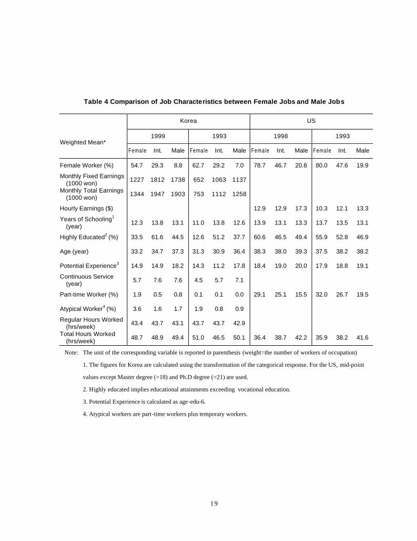
The educational attainment for Korean female jobs is lower than for male jobs. In

contrast, for the US the educational attainment in female jobs is higher than for male jobs.

This patterns is illustrated both for years of schooling and the proportion of employees

exceeding vocational education. However, for both countries, the average (potential) market

experience in female jobs is smaller than in male jobs. At least in Korea, the same is true for

actual experience in the current firm. Part-time and temporary also predominate in female jobs

for both countries. Whereas hours worked are fairly similar between male and female jobs in

Korea, they differ dramatically for the US. Taken together, these findings imply that human

capital at least partially explains the wage gap between male and female jobs.

More detail is given in Tables 6 and 7. As can be seen, Korean female jobs require

relatively fewer general and job-specific vocational skills. However, in the US while female

jobs require less job-specific skills, they require more general skills. Also in contrast to Korea,

US female jobs require more prowess in relating to people (FP) and data (FD). Only the

degree of difficulty in tasks relating to things (FT) is higher in male jobs, as it is in Korea.

Also, in Korea males work in a slightly harsher environment. Certainly for the US, these

attribute differences underscore the importance native skills and preferences in characterizing

job structure. The findings are consistent with common female stereotypes.

14 For 1995 and 1996, the CPS data shows unusual increments in the average hourly earnings of male workers,

which leads to large decreases in the relative female earnings in those years. The consistency of time-series

earnings information from the CPS during this period is somewhat doubted.

19

Table 4 Comparison of Job Characteristics between Female Jobs and Male Jobs

Korea US

1999 1993 1998 1993 Weighted Mean*

Female Int. Male Female Int. Male Female Int. Male Female Int. Male

Female Worker (%) 54.7 29.3 8.8 62.7 29.2 7.0 78.7 46.7 20.8 80.0 47.6 19.9

Monthly Fixed Earnings (1000 won) 1227 1812 1738 652 1063 1137

Monthly Total Earnings (1000 won) 1344 1947 1903 753 1112 1258

Hourly Earnings ($) 12.9 12.9 17.3 10.3 12.1 13.3

Years of Schooling1 (year) 12.3 13.8 13.1 11.0 13.8 12.6 13.9 13.1 13.3 13.7 13.5 13.1

Highly Educated2 (%) 33.5 61.6 44.5 12.6 51.2 37.7 60.6 46.5 49.4 55.9 52.8 46.9

Age (year) 33.2 34.7 37.3 31.3 30.9 36.4 38.3 38.0 39.3 37.5 38.2 38.2

Potential Experience3 14.9 14.9 18.2 14.3 11.2 17.8 18.4 19.0 20.0 17.9 18.8 19.1

Continuous Service (year) 5.7 7.6 7.6 4.5 5.7 7.1

Part-time Worker (%) 1.9 0.5 0.8 0.1 0.1 0.0 29.1 25.1 15.5 32.0 26.7 19.5

Atypical Worker4 (%) 3.6 1.6 1.7 1.9 0.8 0.9

Regular Hours Worked (hrs/week) 43.4 43.7 43.1 43.7 43.7 42.9

Total Hours Worked (hrs/week) 48.7 48.9 49.4 51.0 46.5 50.1 36.4 38.7 42.2 35.9 38.2 41.6

Note: The unit of the corresponding variable is reported in parenthesis (weight=the number of workers of occupation)

1. The figures for Korea are calculated using the transformation of the categorical response. For the US, mid-point

values except Master degree (=18) and Ph.D degree (=21) are used.

2. Highly educated implies educational attainments exceeding vocational education.

3. Potential Experience is calculated as age-edu-6.

4. Atypical workers are part-time workers plus temporary workers.

20

Table 5 T-Test Results on the Difference between Female Jobs and Male Jobs

Korea US

1999 1993 1998 1993

Female Worker (%) *** *** *** ***

Monthly Fixed Earnings (1000 won) *** *** - -

Monthly Total Earnings (1000 won) *** *** - -

Hourly Earnings ($) - - *** **

Years of Schooling1 (year) * *** *** ***

Highly Educated2 (%) n *** *** ***

Age (year) *** *** * n

Potential Experience3 ** ** *** ***

Continuous Service (year) *** *** - -

Part-time Worker (%) ** ** *** ***

Atypical Worker4 (%) *** n - -

Regular Hours Worked (hrs/week) n ** - -

Total Hours Worked (hrs/week) n *** *** ***

Note: ***=1%, **=5%. *=10% significance level, n=insignificant

21

Table 6 Comparison of Job Characteristics Using the K-DOT in Korea (1999)

Weighted Mean Female Jobs Integrated Jobs Male Jobs t-testa General Educational Development (1-6) 3.04 4.00 3.52 *** Specific Vocational Preparation (1-9) 4.94 5.75 6.13 *** Functions Ratings of the tasks performed Relation to Data (0-8) 3.32 4.26 4.32 *** Relation to People (0-8) 1.75 3.56 2.46 * Relation to Things (0-8) 1.80 4.04 3.37 *** Physical Activity

Intensity (0-5) 2.36 2.61 2.38 n Balancing (0-1) 0.02 0.03 0.05 *** Bending (0-1) 0.13 0.09 0.17 n Using Hands (0-1) 0.83 0.97 0.81 n Speaking (0-1) 0.40 0.53 0.37 n Listening (0-1) 0.35 0.20 0.29 n Precise Looking / Perception (0-1) 0.55 0.77 0.61 n

Working Environment Indoor/Outdoor Activity (-1, 0, 1) -0.91 -0.87 -0.67 *** Low Temperature (0-1) 0.01 0.01 0.01 n High Temperature (0-1) 0.04 0.04 0.03 n High Humidity (0-1) 0.05 0.04 0.06 n Noise & Vibration (0-1) 0.13 0.07 0.21 * Injury Dangerousness (0-1) 0.13 0.16 0.31 *** Harmful Atmosphere Condition (0-1) 0.15 0.16 0.21 n

Sources: Korea MOL, Wage Structure Survey, 1999

Korea Manpower Agency Work Information Center, Dictionary of Occupational Titles, 1995.

Note: The rating scale of the corresponding variable is reported in parenthesis.

a. T-test results on the difference between female jobs and male jobs. ***=1%, **=5%. *=10% significance level,

n=insignificant

22

Table 7 Comparison of Job Characteristics Using the US-DOT in the US (1998)

Weighted Mean Female Jobs Integrated Jobs Male Jobs t-testa General Educational Development Reasoning Development (0-5) 2.80 2.39 2.51 ** Mathematical Development (0-5) 1.83 1.42 1.70 n Language Development (0-5) 2.47 1.81 1.98 *** Specific Vocational Preparation (Month) 31.56 29.80 37.57 n Ratings of the tasks performed Relation to Data (0-8) 3.12 2.73 2.83 n Relation to People (0-8) 2.64 1.93 2.00 *** Relation to Things (0-7) 1.70 2.07 2.36 ** Strength Rating (0-4) 0.81 1.19 1.41 *** Guide for Occupational Exploration in terms

of interest requirements Artistic (0-1) 0.02 0.01 0.01 n Scientific (0-1) 0.02 0.02 0.02 n Plants-Animals (0-1) 0.01 0.00 0.06 *** Protective (0-1) 0.00 0.00 0.03 ** Mechanical (0-1) 0.06 0.31 0.37 *** Industrial (0-1) 0.04 0.20 0.18 *** Business Detail (0-1) 0.32 0.07 0.06 *** Selling (0-1) 0.06 0.13 0.06 n Accommodating (0-1) 0.08 0.12 0.03 ** Humanitarian (0-1) 0.15 0.01 0.01 *** Leading-Influencing (0-1) 0.23 0.12 0.17 n Physical performing (0-1) 0.00 0.00 0.00 n

Sources: US BLS, Current Population Surveys, March 1998

_______, Dictionary of Occupational Titles, 4th Ed., 1991

Note: 1.The rating scale of the corresponding variable is reported in parenthesis.

a. T-test on the difference between female jobs and male jobs. ***=1%, **=5%. *=10% significance level,

n=insignificant

23

3. The Effects of Job Characteristics on Wages

In what follows in this section, we confirm for Korea what has been found in the

United States. First, we show that the Korean gender wage gap is significant, but declining.

Second, we show that productivity and job characteristics explain most of the Korean gender

wage gap, but that a significant portion of the gap is associated with earnings function

parameter differences. Third, we confirm that wages are influenced by gender composition.

We show that incumbents in female jobs earn less than incumbents in male jobs. However,

monetarily, we find men to suffer more from being in a woman’s job than women do. Finally,

we show the penalty of being in a woman’s job is mitigated the more one controls for job

characteristics. Because economics and social considerations determine one’s occupation, we

make job choice endogenous in Section 4.

We begin by analyzing the gender wage gap. To assess which of the factors mentioned

in the previous section are important, we decompose earnings in accord with equation (3). The

results are contained in Table 8. We find control variables to explain 52.6% of the 1993 and

51.6% of the 1999 Korean wage gap. Job characteristics explain 11.1 and 11.2%, for each

respective year. Finally, the 36.3% to 37.3% unexplained portions reflect the differing male

and female earnings function coefficients. Some attribute this latter unexplained portion to

discrimination, which they claim is related to the lower observed wages in female occupations.

For this reason we now examine how wages relate to an occupation’s gender composition.

To examine gender composition, we incorporate the PF variable into an earnings

function, as in equation (1). For the United States, Macpherson and Hirsch (1995) show that

24

gender composition effects are reduced by about 25% for women and more than 50% for men

when equation (1) is augmented by skill- related job characteristics. We test this result for

Korean data. We utilize both job characteristics that reflect compensating wage differentials as

well as characteristics reflecting skill-related factors. Working environment variables reflect

compensating factors while the variables GED, SVP, FD, FP, FT, and physical activity reflect

skill-type variables.

Table 9 summarizes how parameter estimates for the percentage female (PF) variable

depend on the included job characteristics. We estimate five different wage specifications.

Specification I regresses the log wages on PF alone. Specification II adds the ordinary control

variables including human capital factors. Specification III adds 1-digit occupation categorical

dummy variables. Specification IV adds the skill-type factors to the model specification.

Finally specification V uses all available information on job characteristics including

compensating factors. Originally the percentage female (PF) is negatively related to wages.

However, incorporating job characteristics remarkably diminishes this inverse relationship.

This decrease in PF’s power suggests that job characteristics may be an important determinant

of wage.

25

Table 8 Decomposition of Gender wage Gap by Specification - Korea

1999 1993

log wages (%) log wages (%) Total log wage gap 0.490 (100.0) 0.617 (100.0) Total explained 0.307 (62.7) 0.393 (63.7)

(1) Ordinary Control Variables 0.253 (51.6) 0.324 (52.6) Productivity-related personal characteristics 0.255 (52.0) 0.322 (52.2) Industry/Establishment -0.002 (-0.5) 0.002 (0.3)

(2) Job characteristics 0.055 (11.2) 0.069 (11.1) Skill-type factors 0.062 (12.7) 0.080 (13.0) Compensating factors -0.008 (-1.6) -0.012 (-1.9)

Unexplained 0.183 (37.3) 0.224 (36.3) Intercept 0.285 (58.1) -0.444 (-72.0) Difference in the coefficients of ordinary control variables 0.035 (7.1) 0.012 (1.9) Difference in the coefficients of job characteristics -0.137 (-27.9) 0.656 (106.4)

Note: The model specification is the same as described in the note to Table 7, except that PF is omitted from the set of

explanatory variables. The calculations are based on Eq. 3.

Table 9 The Effect of the Percentage Female on Wages (θ̂ ) - Korea (1999)

Stepwise Estimation Both Female Male

I. PF Only -0.2665* -0.1666* -0.3349*

II. + Ordinary Control Variables -0.1939* -0.2417* -0.1411*

III. + 1-digit Occupation Dummies -0.1341* -0.2017* -0.0426*

IV. + Job Characteristics (the skill-type factors) 0.0320* -0.0100 0.0519*

V. + Job Characteristics (the compensating factors ) -0.0005 -0.0902* 0.0418*

Note: 1. The ordinary control variables include educational attainments, years of continuous service and the square,

potential market experience and the square, sex, marital status, employment status, job duty, the degree of skill,

union, industry dummies, the size of employment. Job characteristics variables measured at the occupation level are

GED, SVP, FD, FP, FT, physical activity (skill-type factors), and working environment (compensating factors).

2. * means statistically significant at the level of 5%

26

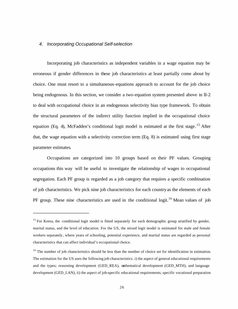
4. Incorporating Occupational Self-selection

Incorporating job characteristics as independent variables in a wage equation may be

erroneous if gender differences in these job characteristics at least partially come about by

choice. One must resort to a simultaneous-equations approach to account for the job choice

being endogenous. In this section, we consider a two-equation system presented above in II-2

to deal with occupational choice in an endogenous selectivity bias type framework. To obtain

the structural parameters of the indirect utility function implied in the occupational choice

equation (Eq. 4), McFadden’s conditional logit model is estimated at the first stage.15 After

that, the wage equation with a selectivity correction term (Eq. 8) is estimated using first stage

parameter estimates.

Occupations are categorized into 10 groups based on their PF values. Grouping

occupations this way will be useful to investigate the relationship of wages to occupational

segregation. Each PF group is regarded as a job category that requires a specific combination

of job characteristics. We pick nine job characteristics for each country as the elements of each

PF group. These nine characteristics are used in the conditional logit.16 Mean values of job

15 For Korea, the conditional logit model is fitted separately for each demographic group stratified by gender,

marital status, and the level of education. For the US, the mixed logit model is estimated for male and female

workers separately, where years of schooling, potential experience, and marital status are regarded as personal

characteristics that can affect individual’s occupational choice.

16 The number of job characteristics should be less than the number of choice set for identification in estimation.

The estimation for the US uses the following job characteristics. i) the aspect of general educational requirements

and the types; reasoning development (GED_REA), mathematical development (GED_MTH), and language

development (GED_LAN), ii) the aspect of job-specific educational requirements; specific vocational preparation

27

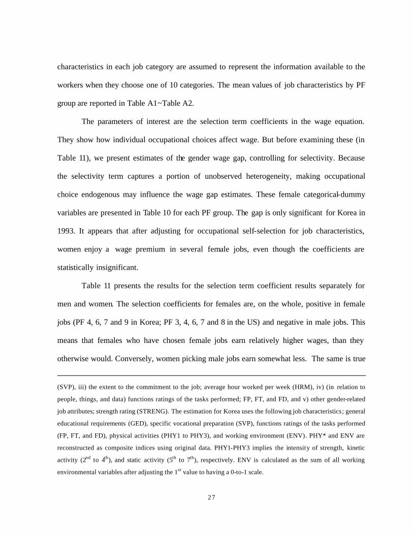
characteristics in each job category are assumed to represent the information available to the

workers when they choose one of 10 categories. The mean values of job characteristics by PF

group are reported in Table A1~Table A2.

The parameters of interest are the selection term coefficients in the wage equation.

They show how individual occupational choices affect wage. But before examining these (in

Table 11), we present estimates of the gender wage gap, controlling for selectivity. Because

the selectivity term captures a portion of unobserved heterogeneity, making occupational

choice endogenous may influence the wage gap estimates. These female categorical-dummy

variables are presented in Table 10 for each PF group. The gap is only significant for Korea in

1993. It appears that after adjusting for occupational self-selection for job characteristics,

women enjoy a wage premium in several female jobs, even though the coefficients are

statistically insignificant.

Table 11 presents the results for the selection term coefficient results separately for

men and women. The selection coefficients for females are, on the whole, positive in female

jobs (PF 4, 6, 7 and 9 in Korea; PF 3, 4, 6, 7 and 8 in the US) and negative in male jobs. This

means that females who have chosen female jobs earn relatively higher wages, than they

otherwise would. Conversely, women picking male jobs earn somewhat less. The same is true

(SVP), iii) the extent to the commitment to the job; average hour worked per week (HRM), iv) (in relation to

people, things, and data) functions ratings of the tasks performed; FP, FT, and FD, and v) other gender-related

job attributes; strength rating (STRENG). The estimation for Korea uses the following job characteristics; general

educational requirements (GED), specific vocational preparation (SVP), functions ratings of the tasks performed

(FP, FT, and FD), physical activities (PHY1 to PHY3), and working environment (ENV). PHY* and ENV are

reconstructed as composite indices using original data. PHY1-PHY3 implies the intensity of strength, kinetic

activity (2nd to 4th), and static activity (5th to 7th), respectively. ENV is calculated as the sum of all working

environmental variables after adjusting the 1st value to having a 0-to-1 scale.

28

for males, but in reverse. For males, the coefficients are somewhat positive in male jobs, but

negative in female jobs. This coefficient implies that men earn relatively more in male jobs,

but relatively less in female jobs.

Table 10 Penalty of Female by PF Group

PF 0 PF 1 PF 2 PF 3 PF 4 PF 5 PF 6 PF 7 PF 8 PF 9 Korea1

1999 0.015 0.185** -0.156 -0.122 -0.114 -0.223** 0.126 0.202 0.131 -0.022 (0.040) (0.060) (0.137) (0.076) (0.071) (0.062) (0.558) (0.178) (1.023) (0.594)

1993 -0.138* -0.121** -0.140** -0.222 -0.187 -0.208** -0.108 -0.130 -0.466 -1.168* (0.071) (0.041) (0.065) (0.145) (0.163) (0.072) (0.084) (0.159) (0.497) (0.601)

US2 1998 -0.156** -0.410 -0.241 -0.340 -0.281 -0.143 -0.102 0.119 0.153 -0.070

(0.082) (0.301) (1.412) (0.340) (0.205) (0.784) (0.391) (0.198) (0.384) (0.579) 1993 -0.601** 0.399** -0.632 -0.119 -0.221 -0.178 -0.007 0.027 0.126 0.601

(0.089) (0.205) (0.648) (0.214) (0.167) (0.403) (0.718) (0.231) (0.209) (0.420)

Note: The penalty of female is estimated as the parameter of FEMALE dummy variable in Eq. (8). The other information

is the same as the notes in Table 11.

29

Table 11 Estimates of the Selection Effect

PF 0

(0≤PF <. 1 ) PF 1

( .1≤PF <. 2 ) PF 2

( .2≤PF <. 3 ) PF 3

( .3≤PF <. 4 ) PF 4

( .4≤PF <. 5 ) PF 5

( .5≤PF <. 6 ) PF 6

( .6≤PF <. 7 ) PF 7

( .7≤PF <. 8 ) PF 8

( .8≤PF <. 9 ) PF 9

( .9≤PF ≤1) Korea1

Both -0.085** -0.660** -0.301** -0.128** 0.357** 0.161** 0.453* 0.480** 0.324 0.048 (0.035) (0.046) (0.060) (0.044) (0.036) (0.027) (0.248) (0.073) (0.348) (0.159)

Female -0.858** -1.540** -0.534** -0.678** 0.931** -0.082 0.476 0.299** -0.324 0.059** (0.233) (0.163) (0.116) (0.084) (0.101) (0.118) (0.376) (0.092) (0.391) (0.023)

Male 0.493** -0.329** -0.010 0.180* -2.159** 22.720 -0.929 -0.502 -0.544* 0.787 (0.066) (0.098) (0.156) (0.109) (0.247) (17.328) (0.955) (0.653) (0.331) (1.873) US2

Both 0.050 0.316 0.287 0.456** 0.365** 0.222 0.270* 0.406** 0.401** 0.010 (0.204) (0.220) (0.508) (0.185) (0.139) (0.273) (0.153) (0.130) (0.146) (0.196)

Female -1.014 -7.532 -10.421** 1.868* 2.083* -6.379** 1.118 7.202** 4.456** -1.171 (7.011) (7.288) (4.920) (1.095) (1.248) (0.079) (1.033) (1.274) (0.672) (0.869)

Male 0.850** -0.071 3.158** 1.337** -0.651** 0.917 -0.196 0.796 -1.513 -2.986 (0.322) (0.311) (0.856) (0.276) (0.312) (1.154) (0.974) (0.774) (1.340) (3.051)

Note: The selection effect is measured as the estimates of ζ in Eq. (8). Adjusted standard errors are in parenthesis. ** and

* indicate statistically significant at the 5% and 10% level, respectively. The standard error in Italic was obtained

from the first stage because the consistent asymptotic covariance matrix of estimates in second stage was collapsed

during the process of the calculation of the adjusted standard error. Other regression coefficients are reported in

Appendix tables. On the job characteristics variables for the conditional logit estimates, refer to the footnote 15.

1. A 1/5 sample of the original WSS was used in this estimation. As the determinants of wages, educational

attainments, years of continuous service and the square, potential market experience and the square, marital status,

employment status, the size of employment, union, and female dummy are considered.

2. A subset of white workers of the CPS was used in order to prevent the result from being disturbed by the race

effect. Educational attainments, potential market experience and the square, SMSA, marital status, employment

status, union, and female dummy are included in the set of determinants of wages.

30

IV. Conclusions

Female labor force participation and wages have been rising in both Korea and the US.

Whereas the degree of occupational segregation has also been declining, jobs in both countries

are still somewhat divided by gender. But at the same time, worker attributes also differ by

gender. Men work longer hours, more years, and get more specific vocational training over

their lifetimes. In the US female jobs require women to relate to people better than things, and

to be more accommodating and humanitarian. In Korea female jobs require women to listen

better, female jobs have far less educational requirements, less physical activity and less harsh

work environments. In simple models, personal and work characteristics account for two-

thirds of the pay gap, but one-third is accounted for by other considerations. Many allege that

discrimination explains this one-third. In particular, they allege that women are relegated to

poor paying jobs, and thus women in general have lower wages because they are crowded into

women’s jobs. In short, they claim occupational segregation is responsible for women’s

inferior economic wellbeing.

31

This study investigated the relationship between occupational sex segregation and

wages. The empirical findings refute the claim that the number of women in one’s occupation

negatively influences wages. Instead, the paper supports hypotheses relating to efficient job

matching. Women choose female jobs to earn a relatively greater amenity package than they

would have received elsewhere. Similarly men choose male jobs to earn relatively more.

To prove our point and elucidate the relationship between occupational segregation

and the gender wage gap, we focused on verifying the importance of job and personal

characteristic s by constructing a two-equation model. One equation modeled job choice and

the other wage determination. We find that once we rigorously define the probability that a

given person (either male or female) is in a particular job, women unambiguously do better in

female jobs and worse in male jobs, while men unambiguously do worse in female jobs.

32

Appendix A:

Korea Dictionary of Occupational Titles

The K-DOT data contains information on general educational development (GED),

specific vocational preparation (SVP), worker functions in relation to data (FD), people (FP),

and things (FT), physical activities, and working environment conditions.

(1) The GED defines six levels on the basis GED defines six levels on the basis of the following:

1. less than 6 years (to such a degree as unschooled or elementary school graduate)

2. 6~ 9 years (to such a degree as junior high school graduate)

3. 9~ 12 years (to such a degree as high school graduate)

4. 12~ 14 years (to such a degree as college graduate)

5. 14~ 16 years (to such a degree as bachelor)

6. more than 16 years (above such a degree as master)

(2) The SVP is divided into the following 9 categories:

1. such a degree as some probation / 2. less than 30 days after probation / 3. 1-3 months /

4. 3-6 months / 5. 6-12 months / 6. 1-2 years / 7. 2-4 years / 8. 4-10 years / 9. more than 10 years

(3) Worker functions (FD, FP, and FT) ahave the following codes:

Data People Things 8 synthesis 8 consultation 8 installation 7 adjustment 7 discussion 7 precision task 6 analysis 6 education 6 regulation 5 collection 5 supervision 5 operation 4 calculation 4 performance 4 manipulation 3 emotion 3 persuasion 3 maintenance 2 comparison 2 transmission report 2 input/output 1 - 1 service assistance 1 transport treatment 0 not concerned 0 not concerned 0 not concerned

The larger the value, the more complicated are the responsibility and the judgment.

(4) Seven measures are introduced for physical activities. The intensity of strength is divided into 5 levels. The larger the

33

value, the more power is needed. For the others, a 1 denotes applicable motion; otherwise they are evaluated at 0.

S L M H VH 1 Intensity of strength very simple work Simple work medium work hard work very hard work

2 Climbing Balancing

4

Reaching hands Using hands Using fingers Touching

5 Speaking 3

Bending Kneeling Crouching Crawling

6 Listening

7

Precise looking the distant things precise looking the close things deep perception the regulation action of the eyes the sense of color vision

(5) Seven categories of working environment are considered. The first is whether or not the workplace is indoor work. Indoor

work is denoted as –1 and outdoor work holds 1. The other items are denoted as 1 if they are applicable; otherwise they are

denoted as 0.

I B O 1 Workplace Indoor both indoor and outdoor outdoor

2 a low temperature or temperature changing 3 a high temperature or temperature changing 4 dampness/high humidity 5 noise / vibration

6 Dangerousness

o mechanism o electricity o burn o explosion o radiation o etc

7 Atmosphere condition

o smell o dust o cloud o gas o bad ventilation o etc

34

Appendix B:

US Dictionary of Occupational Titles

The US-DOT data includes the information on general educational development,

specific vocational preparation, worker functions in relation to data, people, and things,

physical demands (strength rating), and guide for occupational exploration.

(1) General Educational Development (GED) variable denotes aspects of education

that are required for the worker to perform satisfactorily. This is education of a general nature

that does not have a recognized specific occupational objective.

(2) Specific Vocational Preparation (SVP) is defined as the amount of lapsed time

required by a typical worker to learn the techniques, acquire the information, and develop the

facility needed for average performance in a specific job-worker situation.

(3) Every job requires a worker to function to some degree in relation to Data, People,

and Things. The function is arranged in each instance from the relatively simple to the

complex. Each code is determined by the highest appropriate function. The Worker Functions

ratings can be obtained from the middle three digits of the DOT occupational code.

(4) The Physical Demands reflects the estimated overall strength requirement of the

job.

(5) The Guide for Occupational Exploration was designed by the US Employment

Service to provide career counselors and other DOT users with additional information about

the interests, aptitudes, entry- level preparation and other traits required for successful

performance in various occupations. The GOE code is defined in terms of broad interest

requirements of occupations as well as vocational interests of individuals. The twelve interest

areas are defined as follows: Artistic, Scientific, Plants-Animals, Protective, Mechanical,

35

Industrial, Business Detail, Selling, Accommodating, Humanitarian, Leading-Influencing, and

Physical Performing.

36

Table A1 Mean Values of log Wage s and Job Characteristics by PF Group – Korea (1999)

PF Group lnW GED SVP FD FP FT PHY1 PHY2 PHY3 ENVI Both PF 0 7.318 3.439 6.190 4.315 2.422 3.645 2.437 1.036 1.289 0.468

PF 1 7.315 3.628 6.154 4.488 2.568 2.991 2.333 1.031 1.273 -0.107 PF 2 7.279 3.648 5.327 3.246 2.396 3.255 2.470 0.971 1.053 -0.136 PF 3 7.251 3.600 5.156 4.314 2.265 1.273 1.759 0.689 1.034 -0.209 PF 4 6.910 2.755 5.429 3.240 0.990 4.285 2.736 1.217 1.154 -0.108 PF 5 6.724 2.468 4.240 1.973 0.993 1.986 2.978 1.290 1.362 0.762 PF 6 6.911 2.901 4.856 2.839 2.058 1.328 2.713 0.982 2.031 -0.763 PF 7 6.744 2.797 4.836 2.851 1.687 1.924 2.580 1.026 1.419 -0.303 PF 8 6.969 2.592 3.430 2.184 1.793 1.153 2.291 1.153 1.611 -0.534 PF 9 7.200 4.473 6.355 5.705 5.232 1.236 2.000 0.941 2.177 0.000

Female PF 0 7.037 3.439 6.190 4.315 2.422 3.645 2.437 1.036 1.289 0.468 PF 1 6.983 3.628 6.154 4.488 2.568 2.991 2.333 1.031 1.273 -0.107 PF 2 6.990 3.648 5.327 3.246 2.396 3.255 2.470 0.971 1.053 -0.136 PF 3 6.968 3.600 5.156 4.314 2.265 1.273 1.759 0.689 1.034 -0.209 PF 4 6.693 2.755 5.429 3.240 0.990 4.285 2.736 1.217 1.154 -0.108 PF 5 6.519 2.468 4.240 1.973 0.993 1.986 2.978 1.290 1.362 0.762 PF 6 6.828 2.901 4.856 2.839 2.058 1.328 2.713 0.982 2.031 -0.763 PF 7 6.625 2.797 4.836 2.851 1.687 1.924 2.580 1.026 1.419 -0.303 PF 8 6.930 2.592 3.430 2.184 1.793 1.153 2.291 1.153 1.611 -0.534 PF 9 7.198 4.473 6.355 5.705 5.232 1.236 2.000 0.941 2.177 0.000

Male PF 0 7.331 3.439 6.190 4.315 2.422 3.645 2.437 1.036 1.289 0.468 PF 1 7.370 3.628 6.154 4.488 2.568 2.991 2.333 1.031 1.273 -0.107 PF 2 7.367 3.648 5.327 3.246 2.396 3.255 2.470 0.971 1.053 -0.136 PF 3 7.407 3.600 5.156 4.314 2.265 1.273 1.759 0.689 1.034 -0.209 PF 4 7.080 2.755 5.429 3.240 0.990 4.285 2.736 1.217 1.154 -0.108 PF 5 7.007 2.468 4.240 1.973 0.993 1.986 2.978 1.290 1.362 0.762 PF 6 7.071 2.901 4.856 2.839 2.058 1.328 2.713 0.982 2.031 -0.763 PF 7 7.061 2.797 4.836 2.851 1.687 1.924 2.580 1.026 1.419 -0.303 PF 8 7.107 2.592 3.430 2.184 1.793 1.153 2.291 1.153 1.611 -0.534 PF 9 7.265 4.473 6.355 5.705 5.232 1.236 2.000 0.941 2.177 0.000

37

Table A2 Mean Values of log Wages and Job Characteristics by PF Group – US (1998)

PF Group lnW GED GED_MTHGED_LAN SVP HRM FP FT FD STRENG Both PF 0 2.481 2.272 1.417 1.489 31.958 42.330 1.095 4.218 2.119 1.984

PF 1 2.446 2.386 1.591 1.833 37.778 42.113 1.906 2.491 2.691 1.498 PF 2 2.671 3.022 2.178 2.767 40.845 42.947 2.766 2.337 3.327 0.969 PF 3 2.618 2.713 1.939 2.338 45.354 42.080 2.278 0.731 3.345 0.991 PF 4 2.352 2.684 1.777 2.190 37.118 40.121 2.875 1.575 3.614 1.088 PF 5 2.541 3.107 2.119 2.740 49.585 40.040 3.440 1.016 3.465 0.769 PF 6 2.371 3.081 2.146 2.826 46.858 37.939 2.803 0.967 3.565 0.738 PF 7 2.145 2.471 1.624 1.985 19.955 34.275 2.350 1.575 2.998 0.877 PF 8 2.250 2.630 1.602 2.383 24.578 37.169 2.678 1.394 2.498 1.084 PF 9 2.263 2.746 1.707 2.462 25.099 35.035 2.170 2.818 2.937 0.654

Female PF 0 2.348 2.272 1.417 1.489 31.958 42.330 1.095 4.218 2.119 1.984 PF 1 2.227 2.386 1.591 1.833 37.778 42.113 1.906 2.491 2.691 1.498 PF 2 2.551 3.022 2.178 2.767 40.845 42.947 2.766 2.337 3.327 0.969 PF 3 2.449 2.713 1.939 2.338 45.354 42.080 2.278 0.731 3.345 0.991 PF 4 2.199 2.684 1.777 2.190 37.118 40.121 2.875 1.575 3.614 1.088 PF 5 2.435 3.107 2.119 2.740 49.585 40.040 3.440 1.016 3.465 0.769 PF 6 2.283 3.081 2.146 2.826 46.858 37.939 2.803 0.967 3.565 0.738 PF 7 2.111 2.471 1.624 1.985 19.955 34.275 2.350 1.575 2.998 0.877 PF 8 2.223 2.630 1.602 2.383 24.578 37.169 2.678 1.394 2.498 1.084 PF 9 2.258 2.746 1.707 2.462 25.099 35.035 2.170 2.818 2.937 0.654

Male PF 0 2.486 2.272 1.417 1.489 31.958 42.330 1.095 4.218 2.119 1.984 PF 1 2.486 2.386 1.591 1.833 37.778 42.113 1.906 2.491 2.691 1.498 PF 2 2.712 3.022 2.178 2.767 40.845 42.947 2.766 2.337 3.327 0.969 PF 3 2.705 2.713 1.939 2.338 45.354 42.080 2.278 0.731 3.345 0.991 PF 4 2.468 2.684 1.777 2.190 37.118 40.121 2.875 1.575 3.614 1.088 PF 5 2.667 3.107 2.119 2.740 49.585 40.040 3.440 1.016 3.465 0.769 PF 6 2.532 3.081 2.146 2.826 46.858 37.939 2.803 0.967 3.565 0.738 PF 7 2.264 2.471 1.624 1.985 19.955 34.275 2.350 1.575 2.998 0.877 PF 8 2.399 2.630 1.602 2.383 24.578 37.169 2.678 1.394 2.498 1.084 PF 9 2.374 2.746 1.707 2.462 25.099 35.035 2.170 2.818 2.937 0.654

38

Table A3 Parameter Estimates of the Conditional Logit Model by Demographic Group – Korea

(1999)

Single Married Non-Graduates College Graduates Non-Graduates College Graduates

Estimate Std. Err. Estimate Std. Err. Estimate Std. Err. Estimate Std. Err. [Female] GED -2.721* 0.462 -4.923* 0.174 0.567* 0.637 -2.721 0.462 SVP -3.171* 0.616 -5.670* 0.286 2.442* 0.741 -3.171* 0.616 FD 5.351* 0.681 7.710* 0.288 -1.208* 0.800 5.351 0.681 FP 1.016* 0.282 2.359* 0.108 -0.363* 0.383 1.016 0.282 FT -0.440* 0.082 -0.824* 0.047 -0.653* 0.108 -0.440* 0.082 PHY1 10.475* 1.526 16.210* 0.597 -1.935* 1.715 10.475 1.526 PHY2 -6.091* 1.123 -7.262* 0.454 1.073* 1.238 -6.091 1.123 PHY3 -5.364* 0.617 -7.886* 0.236 -1.262* 0.763 -5.364 0.617 ENVI -1.416* 0.138 -1.208* 0.067 -0.364* 0.172 -1.416* 0.138 N 12153 2052 10214 1527 -2 LOG L Model χ2

52302.8 3663.8

8354.3 1095.5

42060.6 4976.6

6099.5 932.6

[Male] GED 8.097* 0.398 2.749 62.285 6.425* 0.288 8.100* 0.578 SVP 13.684* 0.644 1.810 192.609 18.880* 0.580 23.795* 1.215 FD -12.164* 0.669 4.301 237.951 -17.025* 0.591 -21.773* 1.263 FP -6.796* 0.284 -3.175 44.887 -6.520* 0.229 -7.236* 0.459 FT -1.605* 0.062 -2.109* 0.497 -1.922* 0.055 -2.272* 0.113 PHY1 -24.680* 1.366 19.051 580.455 -34.153* 1.170 -42.238* 2.570 PHY2 17.347* 0.891 -21.793 434.664 20.229* 0.729 21.962* 1.651 PHY3 9.306* 0.511 -5.789 179.226 10.581* 0.400 11.873* 0.851 ENVI 2.398* 0.086 0.756 20.706 3.382* 0.066 3.129* 0.143 N 10824 5871 35061 18627 -2 LOG L Model χ2

38531.3 11315.0

17755.2 9281.7

104553.4 56908.4

51598.0 34182.5

Note: * indicates statistically significant at the 1% level.

39

Table A4 Parameter Estimates of Mixed Logit Model – US (1998)

[ γ, For Job Characteristics]

Female Male Parameter Estimate

Standard Error

Wald Chi-Square

Parameter Estimate

Standard Error

Wald Chi-Square

GED_REA -7.828* 3.678 4.531 2.132* 1.729 1.521 GED_MTH -2.275* 1.367 2.771 1.929* 1.424 1.836 GED_LAN 2.036* 1.443 1.992 -4.875* 0.953 26.176 SVP 0.073* 0.031 5.645 -0.050* 0.017 8.393 HRM -0.404* 0.072 31.867 0.018* 0.064 0.080 FP -0.078* 0.407 0.037 -0.909* 0.225 16.308 FT -0.038* 0.217 0.030 -0.573* 0.148 14.956 FD 2.130* 0.270 62.371 2.742* 0.267 105.504 STRENG 0.933* 0.538 3.010 4.214* 0.861 23.923 -2 LOG L Model χ2

97759.251 12373.39 with 36 DF (p=0.0001)

100395.855 18647.79 with 36 DF (p=0.0001)

[ δ, For Individual Characteristics]

Female Male JOB=j1 Education Experience Marital Status Education Experience Marital Status

PF 0 -0.153* -0.006* -0.518* -0.272* 0.009* 0.698* PF 1 -0.160* -0.012* -0.127* -0.208* 0.006* 0.752* PF 2 0.129* -0.010* -0.224* 0.004* 0.014* 0.581* PF 3 -0.006* 0.004* -0.235* -0.096* 0.016* 0.593* PF 4 -0.082* -0.001* -0.211* -0.163* 0.002* 0.467* PF 5 0.080* 0.004* -0.073* 0.026* 0.020* 0.441* PF 6 0.027* -0.004* -0.207* 0.010* -0.001* 0.361* PF 7 -0.095* -0.024* -0.417* -0.112* -0.013* -0.183* PF 8 -0.007* 0.003* -0.204* -0.019* 0.011* -0.179*

Note: 1. The base occupation is PF 90%+, thus the dependent variable is ln [P(JOB=j | JC)/P(JOB=PF9 | JC)].

2. * indicates statistically significant at the 5% level.

40

Table A5 Parameter Estimates at the Second Stage OLS – Korea (1999)

PF 0 PF 1 PF 2 PF 3 PF 4 PF 5 PF 6 PF 7 PF 8 PF 9 INTERCEP 6.487* 6.965* 7.043* 6.353* 5.521* 6.104* 5.295* 5.345* 5.552* 6.372* (0.005) (0.006) (0.012) (0.007) (0.009) (0.010) (0.013) (0.010) (0.023) (0.013) EDU3 0.174* 0.313* 0.246* 0.415* 0.173* 0.191* 0.312* 0.225* 0.098* -0.089* (0.011) (0.008) (0.014) (0.011) (0.014) (0.013) (0.064) (0.015) (0.032) (0.019) EDU4 0.404* 0.498* 0.421* 0.528* 0.371* 0.473* 0.380* 0.394* 0.177 0.081 (0.037) (0.020) (0.013) (0.013) (0.011) (0.017) (0.135) (0.063) (0.235) (0.251) EDU5 0.695* 0.769* 0.635* 0.793* 0.553* 0.558* 0.421* 0.537* 0.277* 0.206* (0.021) (0.022) (0.047) (0.028) (0.025) (0.025) (0.030) (0.028) (0.068) (0.048) TEN 0.061* 0.072* 0.062 0.062 0.084* 0.062 0.072* 0.077* 0.072 0.071 (0.022) (0.026) (0.075) (0.044) (0.027) (0.034) (0.031) (0.029) (0.068) (0.052) TENSQ -0.001 -0.001 -0.001 -0.001 -0.002 -0.001 -0.001 -0.002 -0.002 -0.002 (0.001) (0.001) (0.002) (0.001) (0.001) (0.001) (0.002) (0.001) (0.003) (0.003) EXP 0.024* 0.027* 0.007* 0.017* 0.008* 0.005* 0.002 -0.007* 0.012* 0.014* (0.001) (0.001) (0.002) (0.002) (0.002) (0.002) (0.004) (0.003) (0.005) (0.003) EXPSQ -0.001* 0.000* 0.000* 0.000* 0.000 0.000 0.000 0.000 0.000 0.000 (0.000) (0.000) (0.000) (0.000) (0.000) (0.000) (0.000) (0.000) (0.000) (0.000) MARR 0.039* 0.084* 0.111* 0.095* 0.000 0.108* -0.066* 0.136* -0.006 -0.011 (0.007) (0.010) (0.022) (0.016) (0.015) (0.011) (0.028) (0.015) (0.044) (0.238) TEMP -0.100* -0.228* -0.238* -0.305* -0.072* -0.257* -0.205* -0.094* -0.370* -0.440 (0.009) (0.012) (0.027) (0.018) (0.023) (0.018) (0.032) (0.020) (0.050) (0.238) PART -0.085* -0.166* -0.412* -0.306* 0.000 -0.154* -0.358* -0.236* -0.157 -0.133 (0.008) (0.013) (0.029) (0.023) (0.022) (0.034) (0.073) (0.026) (0.155) (0.238) SIZE2 -0.007 -0.007 -0.056* 0.019 0.019 -0.061* 0.109* -0.059* -0.090* 0.120* (0.010) (0.013) (0.025) (0.014) (0.028) (0.022) (0.027) (0.018) (0.035) (0.040) SIZE3 0.000 0.028* 0.008 0.059* 0.137* -0.058* 0.116* -0.086* -0.151* 0.181* (0.009) (0.012) (0.025) (0.013) (0.025) (0.021) (0.023) (0.017) (0.034) (0.036) SIZE4 0.011 0.053* 0.140* 0.034* 0.123* -0.042 0.083* -0.102* -0.118* 0.231* (0.009) (0.012) (0.026) (0.013) (0.026) (0.022) (0.025) (0.018) (0.037) (0.037) SIZE5 0.096* 0.164* 0.185* 0.135* 0.217* -0.008 0.073* -0.080* 0.091* 0.434* (0.009) (0.012) (0.025) (0.013) (0.026) (0.022) (0.026) (0.018) (0.037) (0.036) UNION -0.018* -0.015* -0.075* 0.059* 0.046* 0.005* 0.009* 0.052* 0.138* 0.057* (0.000) (0.000) (0.000) (0.000) (0.000) (0.000) (0.000) (0.000) (0.000) (0.000) FEMALE 0.015 0.185* -0.156 -0.122 -0.114 -0.223* 0.126 0.202 0.131 -0.022 (0.040) (0.060) (0.137) (0.076) (0.071) (0.062) (0.558) (0.178) (1.023) (0.594) SEL -0.085* -0.660* -0.301* -0.128* 0.357* 0.161* 0.453 0.480* 0.324 0.048 (0.035) (0.046) (0.060) (0.044) (0.036) (0.027) (0.248) (0.073) (0.348) (0.159) σ 0.361 0.671 0.423 0.366 0.444 0.372 0.528 0.543 0.379 0.239 ρ -0.237 -0.984 -0.712 -0.349 0.804 0.432 0.858 0.883 0.855 0.199 N 32,407 21,450 3,932 13,657 5,972 6,982 3,325 5,624 827 2,153 Adj-R2 0.582 0.6411 0.6684 0.6045 0.6249 0.6109 0.5536 0.6328 0.6645 0.6451

Note: 1. SEL is the estimates of ζ in Eq. (8). σ and ρ are calculated from the parameter of SEL.

2. * indicates statistically significant at the 5% level.

41

Table A6 Parameter Estimates at the Second Stage OLS – US (1998)

PF 0 PF 1 PF 2 PF 3 PF 4 PF 5 PF 6 PF 7 PF 8 PF 9 INTERCEP 0.994* 0.477* -0.411* -0.277* 0.123* 0.323* 0.300* 0.225* -0.215* 0.483* (0.014) (0.007) (0.033) (0.005) (0.004) (0.016) (0.007) (0.005) (0.004) (0.005) EDU 0.069 0.072 0.134 0.121* 0.097* 0.094* 0.093 0.076 0.089 0.105 (0.287) (0.151) (0.219) (0.059) (0.022) (0.036) (0.049) (0.081) (0.111) (0.263) EXP 0.033 0.030 0.038 0.034 0.030 0.027 0.024 0.020 0.026 0.024 (0.023) (0.031) (0.036) (0.019) (0.020) (0.025) (0.023) (0.028) (0.022) (0.027) EXPSQ -0.0005 -0.0005 -0.0006 -0.0004 -0.0004 -0.0004 -0.0004 -0.0004 -0.0003 -0.0004 (0.014) (0.021) (0.034) (0.018) (0.018) (0.023) (0.021) (0.017) (0.019) (0.017) SMSA 0.137* 0.225* 0.306* 0.203* 0.161* 0.208* 0.099 0.132* 0.167* 0.177* (0.032) (0.051) (0.100) (0.053) (0.065) (0.053) (0.066) (0.057) (0.042) (0.061) UNION 0.240* 0.295* 0.095* -0.044* 0.148* 0.059* 0.079* 0.111* 0.301* 0.111* (0.002) (0.003) (0.004) (0.002) (0.002) (0.003) (0.003) (0.002) (0.002) (0.002) PART -0.143* -0.293* -0.227* -0.275* -0.230* -0.215* -0.243* -0.196* -0.176* -0.130* (0.000) (0.000) (0.000) (0.000) (0.000) (0.000) (0.000) (0.000) (0.000) (0.000) MARR 0.192* 0.183* 0.115* 0.157* 0.105* 0.144* 0.108* 0.048* 0.046* 0.060* (0.020) (0.032) (0.050) (0.024) (0.023) (0.029) (0.025) (0.018) (0.023) (0.019) FEMALE -0.156 -0.410 -0.241 -0.340 -0.281 -0.143 -0.102 0.119 0.153 -0.070 (0.082) (0.300) (1.412) (0.339) (0.204) (0.784) (0.391) (0.197) (0.383) (0.579) SEL 0.050 0.316 0.287 0.456* 0.365* 0.222 0.270 0.406* 0.401* 0.010 (0.204) (0.220) (0.508) (0.185) (0.139) (0.273) (0.153) (0.129) (0.146) (0.196) σ 0.604 0.696 0.883 0.821 0.731 0.676 0.653 0.706 0.681 0.643 ρ 0.083 0.454 0.325 0.556 0.499 0.329 0.413 0.575 0.589 0.015 N 7,616 3,715 2,840 7,614 5,751 3,547 3,620 5,588 3,644 5,830 Adj-R2 0.2102 0.2855 0.2180 0.3093 0.3119 0.2243 0.2788 0.2587 0.2746 0.1740

Note: 1. SEL is the estimates of ζ in Eq. (8). σ and ρ are calculated from the parameter of SEL.

2. * indicates statistically significant at the 5% level.

42

References

Anker, R. (1998). Gender and jobs: Sex segregation of occupations in the world. Geneva: ILO.

Becker, G. S. (1985). Human capital, effort, and the sexual division of labor. Journal of Labor

Economics, 3(1, Part 2), s33-58.

Beller, A. H. (1982). Occupational segregation by sex: Determinants and changes. Journal of

Human Resources, 17(3), 371-392.

Bergmann, B. R. (1974). Occupational segregation, wages and profits when employers

discriminate by race and sex. Eastern Economic Journal, 1(1-2), 103-110.

Blau, F. D. (1984). Discrimination against women: theory and evidence. Labor Economics:

Modern Views (pp. 53-89). Boston: Kluwer-Nijhoff.

Blau, F. D., Simpson, P., & Anderson, D. (1998). Continuing progress? Trends in

occupational segregation in the United States over the 1970s and 1980s. Feminist

Economics, 4(3), 29-71.

Boskin, M. J. (1974). A conditional logit model of occupational choice. Journal of Political

Economy, 82(2, Part 1), 389-398.

Brink, M., & Willemsen, T. (1997). Work, gender and identity: An exploration of gender(ed)

identities of women and men in relation to participation in paid and household work. In

K. Tijdens, A. Doorne-Huiskes, & T. Willemsen (Ed.), Time allocation and gender

(pp. 31-46). Netherlands: Tilburg University Press.

43

England, P. (1989). A feminist critique of rational-choice theories: implications for sociology.

American Sociology, 20(1), 14-28.

Filer, R. K. (1989). Occupational segregation, compensating differentials, and comparable

worth. Pay equity: Empirical inquiries (pp. 153-170). Washington, D.C.: National

Academy Press.

Flyer, F. A. (1997). The influence of higher moments of earnings distributions on career

decisions. Journal of Labor Economics, 15(4), 689-713.

Fuchs, V. R. (1971). Differences in hourly earnings between men and women. Monthly Labor

Review, 94(5), 9-15.

Hwang, S. K. (2001). Does "femaleness" reduce wages?: An analysis of the effect of gendered

comparative advantage on occupational segregation and gender wage gap. Dissertation

in SUNY (Binghamton).

Jacobs, J. A. (1999). The sex segregation of occupations: Prospects for the 21st century. In G.

N. Powell (Eds.), Handbook of Gender in Organizations (pp. 125-141). Newbury Park,

CA: SAGE.

Killingsworth, M. R. (1987). Heterogeneous preferences, compensating wage differentials,

and comparable worth. Quarterly Journal of Economics, 102(4), 727-742.

Lee, L. (1983). Generalized econometric models with selectivity. Econometrica, 51(2), 507-

512.

Macpherson, D. A., & Hirsch, B. T. (1995). Wages and gender composition: Why do women's

jobs pay less?. Journal of Labor Economics, 13(3), 426-471.

44

McFadden, D. (1973). Conditional logit analysis of qualitative choice behavior. In P.

Zarembka (Ed.), Frontiers in Econometrics. New York: Academic.

Oaxaca, R. L. & Ransom, M. R. (1994). On discrimination and the decomposition of wage

differentials. Journal of Econometrics, 61(1), 5-22.

Osterman, P. (Ed.) (1984). Internal labor markets. Cambridge: MIT Press

Polachek, S. W. (1975). Potential biases in measuring male-female discrimination. Journal of

Human Resources, 10, 205-229.

Polachek, S. W. (1981). Occupational self-selection: A human capital approach to sex

differences in occupational structure. Review of Economics and Statistics, 63(1), 60-

69.

Polachek, S. W. (1985) Occupational Segregation: A Defense of Human Capital Predictions,

Journal of Human Resources, 20(1), 437-40.

Polachek, S. W. (1987). Occupational segregation and the gender wage gap. Population

Research and Policy Review, 6, 47-67.

Polachek, S. W. (1995) Human Capital and the Gender Earnings Gap: A Response to Feminist

Critiques, in Out of the Margin: Feminist Perspectives on Economic Theory, (E.

Kuiper and J. Sap, eds.) Routeledge Press, 1995

Sorenson, E. (1990). The crowding hypothesis and comparable worth issue. Journal of Human

Resources, 25(1), 55-89.